LUCAS Copernicus 2018: Earth-observation-relevant in situ data on land cover and use throughout the European Union

The Land Use/Cover Area frame Survey (LUCAS) is an evenly spaced in situ land cover and land use ground survey exercise that extends over the whole of the European Union. LUCAS was carried out in 2006, 2009, 2012, 2015, and 2018. A new LUCAS module specifically tailored to Earth observation (EO) was introduced in 2018: the LUCAS Copernicus module. The module surveys the land cover extent up to 51 m in four cardinal directions around a point of observation, offering in situ data compatible with the spatial resolution of high-resolution sensors. However, the use of the Copernicus module being marginal, the goal of the paper is to facilitate its uptake by the EO community. First, the paper summarizes the LUCAS Copernicus protocol to collect homogeneous land cover on a surface area of up to 0.52 ha. Secondly, it proposes a methodology to create a ready-to-use dataset for Earth observation land cover and land use applications with high-resolution satellite imagery. As a result, a total of 63 364 LUCAS points distributed over 26 level-2 land cover classes were surveyed on the ground. Using homogeneous extent information in the four cardinal directions, a polygon was delineated for each of these points. Through geospatial analysis and by semantically linking the LUCAS core and Copernicus module land cover observations, 58 426 polygons are provided with level-3 land cover (66 specific classes including crop type) and land use (38 classes) information as inherited from the LUCAS core observation. The open-access dataset supplied with this paper (https://doi.org/10.6084/m9.figshare.12382667.v4 d'Andrimont, 2020) provides a unique opportunity to train and validate decametric sensor-based products such as those obtained from the Copernicus Sentinel-1 and Sentinel-2 satellites. A follow-up of the LUCAS Copernicus module is already planned for 2022. In 2022, a simplified version of the LUCAS Copernicus module will be carried out on 150 000 LUCAS points for which in situ surveying is planned. This guarantees a continuity in the effort to find synergies between statistical in situ surveying and the need to collect in situ data relevant for Earth observation in the European Union.

1 Introduction

The Land Use/Cover Area frame Survey (LUCAS) is an evenly spaced in situ land cover and land use data collection exercise that extends over the whole of the European Union (EU) (Gallego and Delincé, 2010; Eurostat, 2018c). LUCAS has been carried out in 2006, 2009, 2012, 2015, and 2018. During these five campaigns, a total of 1 351 293 points at 651 780 unique locations were surveyed and 5.4 million photos were collected. On each of these surveyed points, observations were recorded on up to 109 variables. The combination of the information collected in the five LUCAS surveys has resulted in the most comprehensive in situ database on land cover and land use in the EU (d'Andrimont et al., 2020).

LUCAS in situ data collection was designed for EU-wide standardized reporting of land cover and land use area statistics and not for training and validation of remote sensing data algorithms. The LUCAS activity is complementary to the CORINE Land Cover (CLC) inventory that collects land cover data by interpreting satellite images and orthophotos. In addition, in 2018 the Copernicus High Resolution Layers (HRL) were produced to provide information about different land cover characteristics. Five HRLs describe some of the main land cover characteristics: impervious (sealed) surfaces (e.g., roads and built-up areas), forest areas, grasslands, water and wetlands, and small woody features.

In the scientific community, LUCAS has been widely used for soil studies thanks to the topsoil survey module (Orgiazzi et al., 2018). LUCAS data have also already been valuable in the context of land cover and land use research and remote sensing specifically. Esch et al. (2014) used the data for crop-type mapping in the north of Germany. Zillmann et al. (2014) provided an accuracy assessment of grassland mapping in Hungary based on LUCAS. Mack et al. (2017) used Landsat time series along with LUCAS in situ data to generate a land use and land cover product for Germany. Leinenkugel et al. (2019) assessed the potential of open geodata including LUCAS to generate land use and land cover products from multi-temporal Landsat satellite observations over three European sites. Pflugmacher et al. (2019) recently demonstrated the potential of using LUCAS to map pan-European land cover (13 classes) with Landsat data. Close et al. (2018) provided a Sentinel-2 LUCAS-based classification over southern Belgium in the context of Land Use, Land-Use Change, and Forestry (LULUCF) monitoring. According to Weigand et al. (2020), LUCAS in situ data are a suitable source for classifying high-resolution Sentinel-2 imagery at a large scale. Weigand et al. (2020) tested the accuracy of different pre-processing approaches of the LUCAS data based on positioning and semantic selection. These studies highlight that there is an interest and value to the remote sensing research community in using LUCAS in situ data. Nevertheless, the LUCAS core protocol has major limitations in terms of spatial scale and representativeness when it comes to collecting in situ data for calibration, training, and/or validation of EO products.

While LUCAS survey data had been valuable in providing in situ observations relevant for remote sensing as highlighted, the LUCAS survey was designed to collect statistics and thus has inherent shortcomings when used in the context of EO. In 2018, a new “LUCAS module” specifically tailored to Earth observation (EO) was introduced: the “LUCAS Copernicus module” (words in quotation marks are defined in the glossary in Appendix B). The Copernicus module was designed to improve the value of LUCAS in situ surveying for EO for three specific reasons described hereafter.

First, in situ observations recorded with a high precision are needed to ensure the quality of EO applications and the development of services relying on geo-location. Second, the collection of the in situ data has to be done through protocols that are compatible with decametric sensors. Specifically, the spatial extent of the observation needs to be designed according to the spatial resolution of common EO sensors. Third, the diversity of land cover and land use in the EU needs to be represented in the thematic diversity of the information collected in situ. Comprehensive and thematically rich in situ data can lead to better classifiers and more accurate multi-temporal land surface mapping. Finally, the representative, comprehensive, and precisely geo-located in situ data available over larger areas need to be made available with an open-access license.

Free and open accessibility is in fact essential for contributing to the creation of common in situ datasets and protocols as currently pursued by, for example, the Land Product Validation (LPV) of the Working Group on Calibration and Validation of the Committee on Earth Observation Satellites (CEOS) and by the Joint Experiment for Crop Assessment and Monitoring (JECAM). The availability of such datasets acquired with transparent protocols is key to assess the quality of EO products resulting from various public and commercial activities. Thus, the Copernicus module gives the opportunity to further integrate the classical LUCAS survey purpose of collecting statistically representative information with the need to collect in situ data to produce better EO-derived products, specifically for the EU's Copernicus program. The Copernicus module equips the EU with an in situ dataset specifically fitting EO land application monitoring, allowing the development of consistent land monitoring at the EU level.

While data from the Copernicus module have a been available since 2019, they have not been used in EO applications (to the best of our knowledge). This study is reducing the complexity of the data to ease the uptake of LUCAS Copernicus data by the remote sensing community.

This paper describes and provides the LUCAS Copernicus data in a ready-to-use format. More specifically, this study (i) describes the LUCAS 2018 Copernicus in situ survey protocol, (ii) presents a methodology to produce polygons from the surveyed data to be used in EO studies, (iii) proposes a method to inherit more detailed information from the LUCAS core, and (iv) highlights the added value of the survey in order to derive a simplified protocol for the LUCAS Copernicus module that will be integrated in future LUCAS surveys (e.g., in 2022).

2 LUCAS 2018 data

The survey consists of a two-phase sampling. In the first phase, 1.1 million geo-referenced points are systematically drawn forming a 2×2 km² grid, i.e., one point every 2 km in the EU. The points are then stratified according to land cover classes to allow the second phase of sampling. In 2018, this resulted in 337 854 points for which statistical information is collected by surveyors in the field or by photo interpretation in the office. The sampling design methodology used for the LUCAS 2018 survey is described in detail in Scarnò et al. (2018). The grid is static and includes 1 090 863 points stratified according to land cover class and is available in CSV format from Eurostat (2019b). For a detailed description of the grid data see Eurostat (2018a), and for technical details about the stratification see Eurostat (2018b).

In 2018, the campaign involved more than 1300 actors including more than 900 surveyors and lasted for 23 months. The actual in situ data collection occurred between March and September 2018. The raw data have been available online since May 2019 (Eurostat, 2019a) as a downloadable CSV table with 97 columns and 337 854 records (Table 4 presents the attribute names of the 97 original fields; a record descriptor is available in Eurostat, 2019c; the detailed survey instructions in Eurostat, 2018d). Out of the 337 854 points surveyed in 2018, 23 % points had been included in three previous surveys (2009, 2012, and 2015), 25 % had already been surveyed once or twice before (e.g., in 2009 and 2015), and the remaining 52 % of the points were new entries. In the LUCAS 2018 survey, 70.45 % of the points were surveyed in situ, and 29.54 % were obtained through the interpretation of detailed ortho-photos (Tables 1 and A1).

Eurostat has carried out LUCAS surveys every 3 years with the survey design ever evolving; however the LUCAS core component (i.e., the identification of the point, and the surveying of specific variables on different aspects of land cover, land use, and land and water management; Eurostat, 2018d) has remained comparable for all five surveys. At each LUCAS point, standard variables are collected including land cover, land use, environmental parameters, and landscape photos. In addition to the core variables collected, other specific modules were carried out on demand such as (i) the transect of 250 m to assess transitions of land cover and existing linear features (2009, 2012, 2015), (ii) the topsoil module (2009, 2012 (partly), 2015, and 2018), (iii) the grassland (2018), and (iv) the Copernicus module (2018).

Out of the 337 854 LUCAS points sampled in 2018 (combining in situ and photo-interpreted points, Table A1), the sample of the Copernicus module was a third-phase sampling nested in the two-phase sampling scheme. The Copernicus module was planned for 90 620 points and actually executed for 63 364 points (Table 1). For 27 256 (30.08 %) planned points, the surveyors did not manage to reach the point to make the observation, for example due to natural or human-made obstacles. Therefore, the Copernicus module was carried out in situ for a total of 63 364 points, thus corresponding to 69.92 % of the planned Copernicus points.

Table 1 LUCAS 2018 points totaling 337 854 points. The points were either surveyed in situ (238 014, 70.45 %), photo-interpreted in the office (99 803, 29.54 %), or not surveyed (i.e., “in situ PI not possible”, “out of national territory”, or “out of EU28”). The Copernicus module was collected for a subset of the in situ points in addition to the LUCAS core protocol collected for any in situ point.

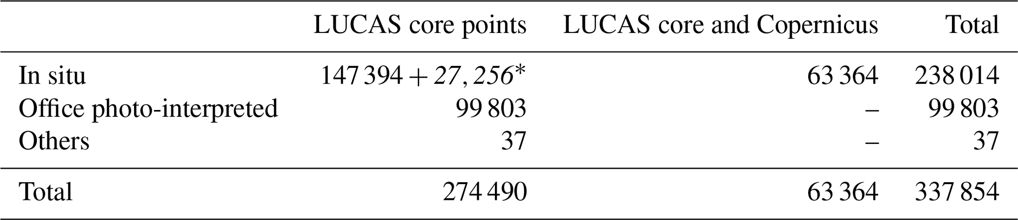
^* Planned in the Copernicus module, but the Copernicus survey was not possible and thus solely surveyed as a point.

3 LUCAS 2018 Copernicus protocol

In the LUCAS core protocol, the surveyor aims to get as close as possible to the theoretical point. The surveyor then provides the so-called LUCAS core observations for the “LUCAS theoretical grid” point from the location that the surveyor was actually able to reach. Thus, although typically close to each other, the nominal geolocation of a LUCAS point may not exactly coincide with the actual observation location, which is not recorded for LUCAS core points. As an illustrative example, the observation is made from an unknown location and assigned to the LUCAS nominal point in red in Fig. 1. The exact geolocation of the surveyor observation is recorded only in the corresponding LUCAS Copernicus entry (green point in Fig. 1). The “LUCAS theoretical grid” point observation is representative for a circle of 1.5 m radius. In some specific cases, the window of observation is extended to a 20 m radius whenever the land cover at the point is heterogeneous (Eurostat, 2018d). This occurs in areas such as permanent crops (B7X, B8X, except nurseries B83) where the parcels of permanent crops contain trees or other plants along with bare soils and/or grassland or another crop; in woodland (CXX); shrubland (DXX) where a mix of, for example, shrubs and trees might occur; in grassland (EXX) where land features may alternate (e.g., grassland with trees); in bare land (FXX); and in wetland (HXX). Given the mentioned protocol, two main drawbacks of the LUCAS core observations are apparent for their use in the context of EO applications.

The first limitation is that the observation corresponds to a fraction (7 %) of a Sentinel-1 and Sentinel-2 pixel (the circle with 1.5 m radius, thus representing an area of 7.07 m²) and is thus not directly usable with such decametric sensors. Indeed, the 10 m pixel (i.e., 100 m²) could be covered by different land covers while the LUCAS observation only captures one. This jeopardizes the use of LUCAS core observations for training and validation when building EO-derived products. The second limitation refers to GPS geo-location survey inaccuracies that are comparable to the representative area, making the information unsuitable. To address these limitations, the LUCAS Copernicus module collected the exact geolocation of the observation as well as information on the spatial extent and homogeneous continuity of the land cover (LC) observed around the point, making it suitable for use in EO applications.

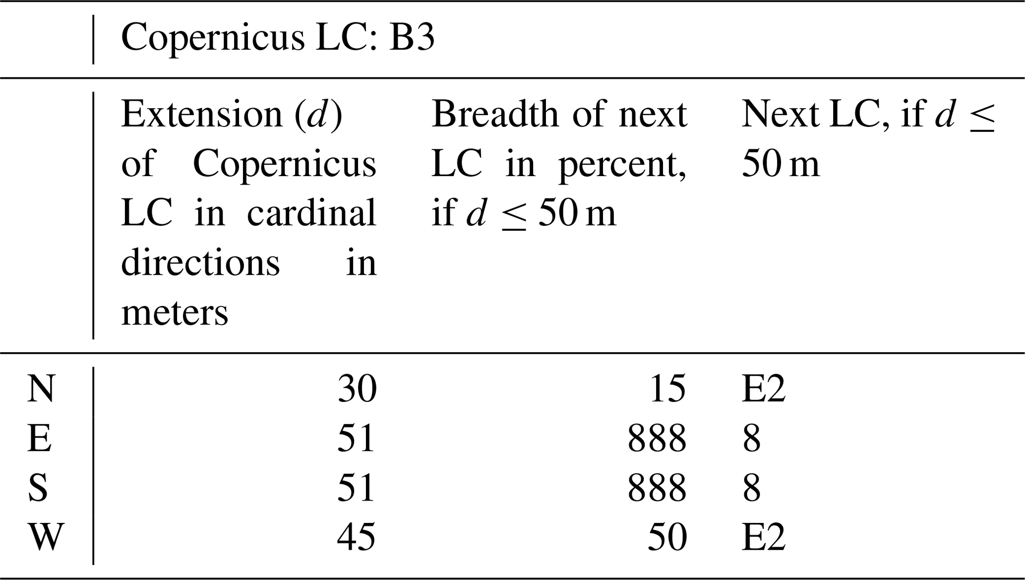
More specifically, the following additional data are collected on the LUCAS Copernicus surveyed points: (i) the measured location of the observation and (ii) the land cover (level-2) extent up to 51 m from the point in the four cardinal directions (N, W, S, E), as well as the neighboring LC. Note that the surveyor records 51 m to indicate that the land cover is homogeneous for more than 50 m. However, as the exact extent is not reported, we conservatively set it to the minimum extent of 51 m. Figure 1 illustrates the Copernicus protocol for one point, and the respective collected data are shown in Table 2. On the basis of these LUCAS Copernicus observations, a quadrilateral polygon with homogeneous LC can be constructed. As part of the Copernicus module, the surveyor collects 13 additional variables and three types of observations (Table 2): the level-2 LC (one variable), the extent of the Copernicus land cover (LUCAS LC classification at level 2) registered at the point reached in the field (four variables), the next land cover (up to 50 m) (four variables), and the breadth of the next land cover (four variables). The breadth corresponds to the percent of the width of the land cover in this sector, as visible on the landscape photo (i.e., landscape photos taken in each cardinal direction: N, E, S, W). This means that the breadth is 100 % if the next LC is seen all over the photo from one side to the other. If the next land cover is not visible on the photo because it is completely behind a linear feature (e.g., hedge) or because it is completely hidden by the terrain, then the next land cover is to be recorded but the breadth is 0 %. For more information about the breadth and the next land cover, see Eurostat (2018d).

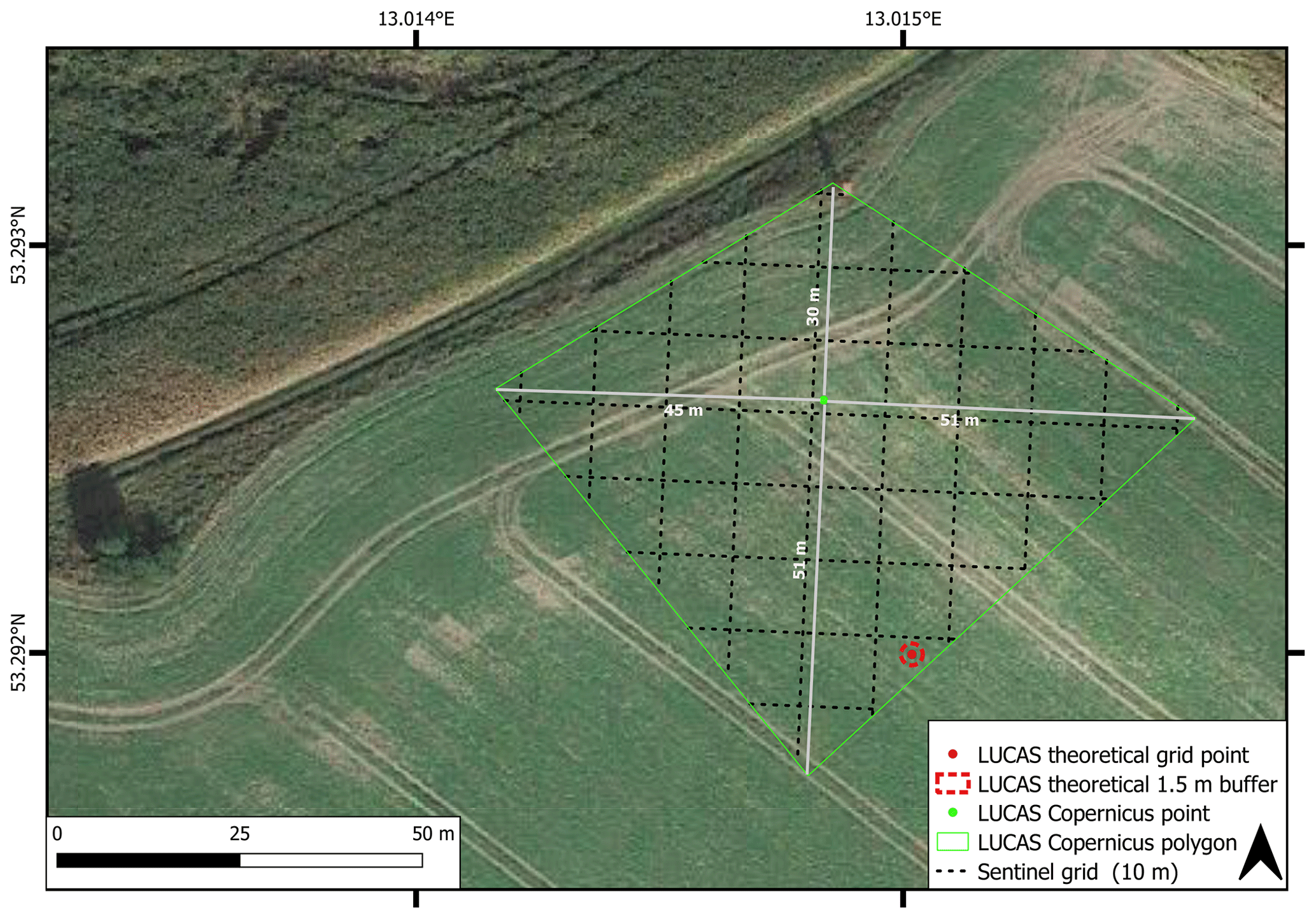
Figure 1 Building the Copernicus polygon geometry (example for point ID 45223358). The collected Copernicus variables (Table 2) are used to build the geometry of the Copernicus polygon. As the LUCAS theoretical point is inside the Copernicus polygon, the LC legend of the LUCAS theoretical observation (here B32 – rape and turnip rape) could be inherited to the Copernicus polygon (B3 – non-permanent industrial crops) as described in Sect. 4. The background RGB imagery is obtained from map data ©2019 Google.

Table 2 Example of information collected by the Copernicus protocol (for point with ID 45223358). The Copernicus protocol collects observations on 13 variables: land cover (LC) at LUCAS legend level 2 (here B3 is “non-permanent industrial crops”), the extension of the LC in the four cardinal directions (up to 50 m, 51 means more than 50 m), the breadth of the next LC in the four cardinal directions (%), and the next LC in the four directions (here, E2 means “grassland without tree/shrub cover” in the N and W). Figure 1 shows how this information is used to build the geometries of the Copernicus polygon with homogeneous LC. The radial distance d is measured between the Copernicus point and the next LC, with “888” and “8” meaning “not relevant”.

The following sections describe how the LUCAS Copernicus data are prepared and cleaned to obtain the ready-to-use dataset provided with this paper. The following workflow was done in R (Code and Data availability; see Sect. 6).

3.1 Adding an explicit LUCAS land cover and land use legend

The LUCAS land cover classification is hierarchical and contains four levels briefly described hereafter (for a detailed description, see the Technical reference document C3 Classification, Eurostat, 2018e). The land cover classification system is subdivided into eight main level-1 land cover categories: artificial land, cropland, woodland, shrubland, grassland, bare land, water, and wetlands. The level-2 legend contains 26 classes (e.g., 8 under level-1 B cropland) and level-3 comprises 73 classes (e.g., 9 under level-2 B1 cereals). Only a limited number of observations have level-4 land cover information distributed into 205 classes (“LC1_SPEC” field in the data). Similarly, the land use comprises 40 subclasses.

To facilitate the usability of the data, in addition to the code describing the land use or land cover (e.g., B21 or U112), an explicit legend label was added to the dataset provided with this paper. This was done by adding nine explicit label fields (Table 4) to the data for the LC and LU legend.

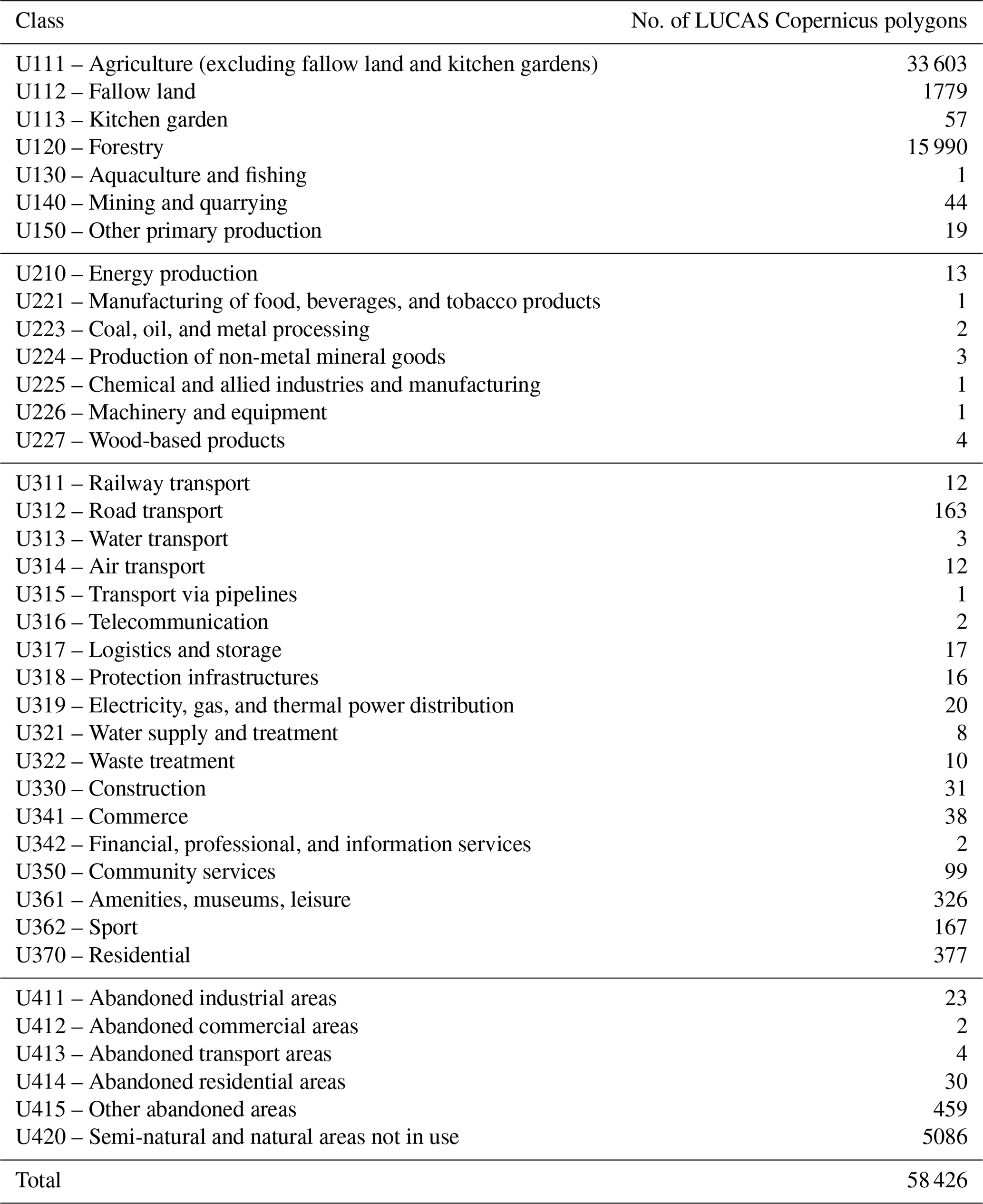
In the results section, details on the hierarchical legend structure classes are also provided (Table 3 on level-2 legend, Fig. 5 on level-3 legend (“LC1” field in the data), and the 40 land use sub classes as shown by the level-3 distribution of the Copernicus polygons in Table A2), “LU1” in the data).

Table 3 Distribution of level-2 land cover classes of the resulting LUCAS Copernicus polygons (N=63 287).

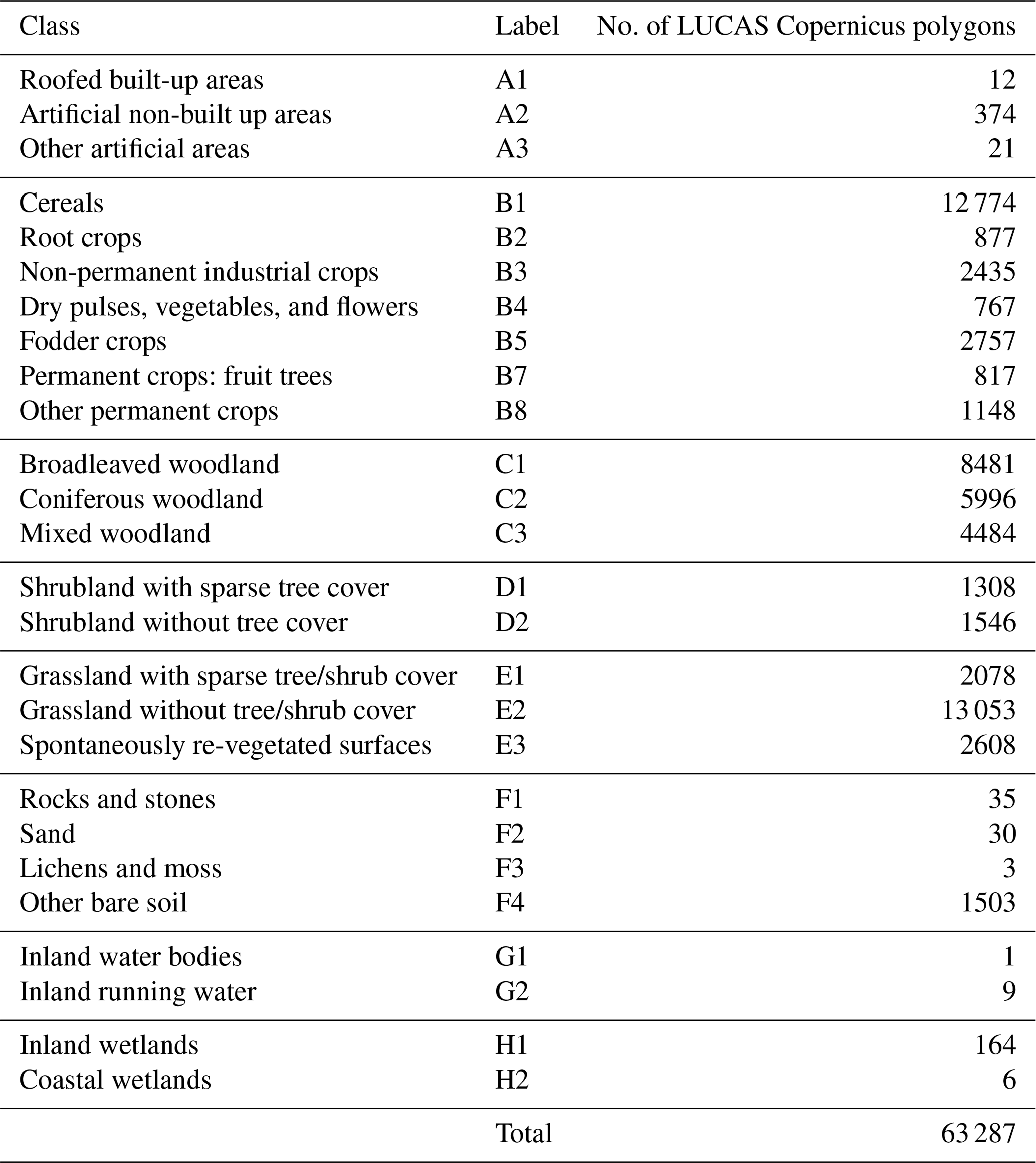
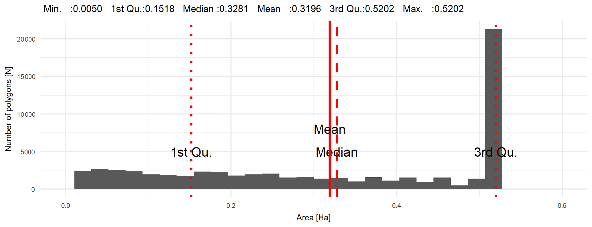
Figure 2 Distribution of the area of the LUCAS Copernicus polygons in hectares (N=63 287). On average, the polygon covers an area of 0.33 ha.

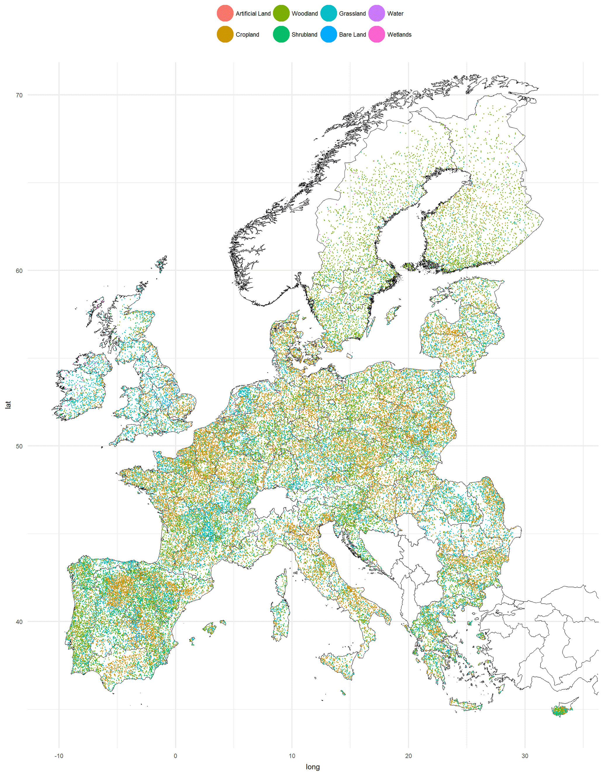
Figure 3 Map of LUCAS Copernicus polygons (N=63 287) surveyed in 2018 per level-1 land cover class over the EU28.

3.2 Constructing the LUCAS Copernicus polygon

On the basis of the LUCAS Copernicus observations, a polygon with homogeneous LC can be constructed. In order to generate the LUCAS Copernicus polygon, the Copernicus point (i.e the effective location of the surveyor, i.e., “GPS_LAT” and “GPS_LONG”) is defined as the center to build a quadrilateral for each point. The location of this point is first projected in the Lambert azimuthal equal-area projection coordinate reference system (ETRS89-LAEA). Second, the four distances (N, W, S, E) measured by the surveyor are added to the point in the four respective cardinal directions, resulting in 63 364 irregular quadrilaterals (Table 1). The quadrilateral diagonals can measure up to 102 m but are smaller if the surveyor found a field boundary within 51 m of the LUCAS Copernicus point.

3.3 Quality check

While the Copernicus protocol was implementable for 63 364 polygons, several surveyed polygon locations (i.e., LUCAS Copernicus polygon as defined by “GPS_LAT” and “GPS_LONG”) were either missing or wrong. The missing locations could be flagged for 67 polygons (“GPS_PREC”=8888, “GPS_LAT”=0, or “GPS_LONG”=0). In addition to these, 10 polygons were discarded because the surveyor geolocation (“GPS_LAT”, “GPS_LONG”) was far away from the nominal location (“TH_LAT” , “TH_LONG”), i.e., difference larger than 0.1^∘ (i.e., about 7.1 km in the center of the EU). In addition to the missing GPS-measured locations, some macro errors were flagged and removed by selecting polygons for which the longitude and latitude differences between the GPS measured location and theoretical location (“TH_LAT” , “TH_LONG”) are larger than 0.1^∘. This allows us to flag and remove 10 polygons which are all wrongly located because of the “GPS_EW” field (i.e., GPS observation east–west). This location quality check permits us to flag and remove a total of 75 polygons resulting in a final total of 63 287 polygons.

3.4 Resulting LUCAS Copernicus data

The 63 287 Copernicus polygons surveyed are published along with this paper. They are distributed among 26 level-2 LC classes (Table 3) in eight level-1 LC classes (see map in Fig. 3).

The homogeneous area of the 63 287 polygons ranges between 0.005 and 0.52 with an average of 0.33 ha (Fig. 2) corresponding to 32 10 m pixels. Half of the polygons are larger than 0.33 ha. Also, the third quartile corresponds to the maximum area of 0.52 ha, which is the maximum area possible for a rhombus with diagonals of 102 m (51 m+51 m). Among the 63 287, it is worth mentioning that 21 657 polygons (i.e., 34.2 %) have an area greater than 0.5 ha, i.e., thus corresponding to almost fifty 10 m pixels depending on the orientation. These characteristics make the obtained spatial data well suited for training and validation of products based on decametric (i.e., 0.01 ha) and even subdecametric remote sensing sensors.

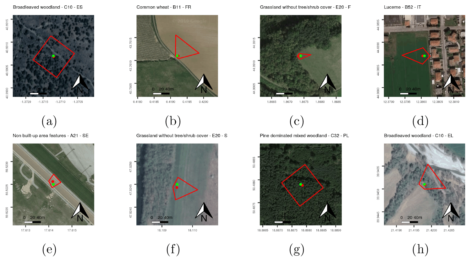
Figure 4 Examples of LUCAS Copernicus built polygons. The green point is the theoretical LUCAS point. The red point is the GPS location of the Copernicus surveyor. Polygons are built using distances in the N, E, S, and W directions collected on the ground. The background RGB imagery is obtained from map data ©2019 Google.

Figure 5 Distribution of level-3 land cover (inherited from LUCAS core) for the LUCAS Copernicus polygons (N=58 426).

4 Linking LUCAS core data to Copernicus polygons

A set of rules were defined to link LUCAS core and LUCAS Copernicus data and thus enrich the LUCAS Copernicus set of information. The rationale is that if the LUCAS theoretical point location falls within the LUCAS polygon, the LUCAS-core-surveyed attributes at the theoretical point could be inherited by the LUCAS Copernicus polygon. This condition is satisfied by the vast majority of the polygons (60 134 points, i.e., 95.02 %). In addition, to filter out suspicious data points where the LUCAS core and Copernicus information were not in agreement despite being spatially consistent, we retained only those points where the reported Copernicus level-2 land cover observed is the same as the one reported for the LUCAS theoretical point (50 417 points, i.e., 95.47 %). This happens when a surveyor can observe the LUCAS theoretical point from a distance but makes the Copernicus observation at the actual point that was reached. At this Copernicus point, the land cover does not correspond to the land cover of the LUCAS theoretical point. Among the 63 287 Copernicus polygons available with this paper, 58 426 polygons (i.e., 92.23 %) fulfill both requirements (condition “CPRN_LC_SAME_LC1” and condition “LUCAS_CORE_INTERSECT” in the provided dataset) and are thus flagged as “COPERNICUS_CLEANED” in the data. For these polygons, the more detailed level-3 land cover class of the LUCAS core can be inherited by the LUCAS Copernicus polygon (“COPERNICUS_CLEANED” is “TRUE”). Figure 4 illustrates the variety in shapes of the constructed quadrilateral Copernicus polygons as projected on top of satellite imagery for different land cover types. The resulting polygons are distributed over 66 specific LC classes as shown in Fig. 5. Similarly, the level-3 land use (LU) is also available distributed in 38 classes organized in four main classes (see Table A2).

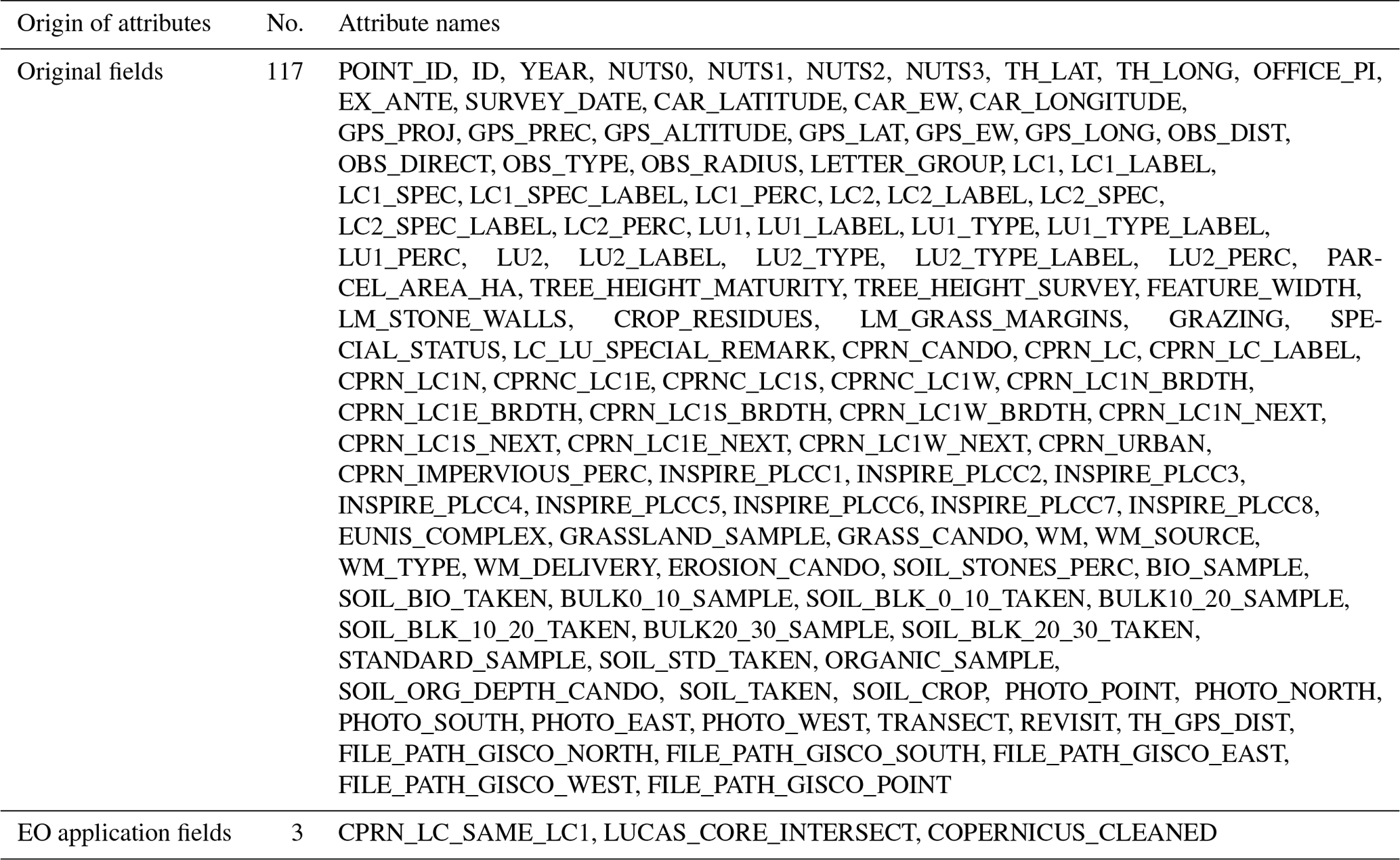
Table 4 The LUCAS Copernicus 2018 dataset is provided as a polygon shapefile along with a table with 120 attributes to be joined based on POINT_ID. Among the 120 attributes, 117 attributes are the original as described in d'Andrimont et al. (2020), and three attributes are obtained as described in Sect. 6.

5 Discussion

The LUCAS Copernicus polygons and data compiled and presented here can provide valuable information for a variety of topics and applications. The LUCAS Copernicus polygons can provide valuable information to extract land-cover-specific surface radiometric and temporal signatures as measured by different sensors, in the multispectral, thermal, and microwave ranges, for different land cover types. This is particularly relevant for land covers exhibiting a dynamic signal (e.g., forests, grasslands, crops) that is modulated by climatic and agroecological conditions, which are well sampled in this EU-wide dataset. As an illustration, the dataset was used by Meroni et al. (2021) to extract crop-specific land surface phenology from Sentinel-1 and Sentinel-2. The dataset can serve various EO-based applications, among many others: train classification algorithms for land cover mapping using existing sensors (e.g., Sentinel 1 and 2, Landsat, QuickBird, ASTER, WorldView), validate land cover products centered on 2018 (e.g., the Copernicus High Resolution Layers), study land-cover-specific land surface processes (e.g., phenology), and develop algorithms to monitor crop and grassland management practices. Future surveys could consider drones to collect high-resolution NADIR view observations concomitant with the survey date. Such data could then be used a posteriori to collect training data for landscape elements difficult to monitor with decametric sensors and could thus provide training data for future research using very high-resolution satellite observations.

With this paper we provide LUCAS Copernicus polygons constructed at 63 287 locations. In addition, we provide a dataset that benefits from inheriting attributes collected at those same points via the LUCAS core protocol. This results in 58 426 Copernicus polygons, discarding a total of 4 861 polygons.

The LUCAS Copernicus module is also planned to be carried out during the LUCAS 2022 survey. However, a simplified protocol has been designed for the LUCAS 2022 survey. In this protocol, the observations on the distance of homogeneous LC from the point and the LC remain, but observations on the neighboring LC and breadth of the neighboring LC have been discarded. Despite this simplification, the coverage of the 2022 LUCAS Copernicus module will be expanded to 150 000 LUCAS points for which in situ surveying is planned.

6 Code and data availability

The data repository https://doi.org/10.6084/m9.figshare.12382667.v4 (d'Andrimont, 2020) contains the following files:

• LUCAS_2018_Copernicus.zip, compressed files containing the dataset;

  • –

    LUCAS_2018_Copernicus_polygons.shp, shapefile of polygons with the “POINT_ID” attribute;

  • –

    LUCAS_2018_Copernicus_attributes.csv, CSV file containing the 120 variables including the “POINT_ID”;

• ESSD_create_LUCAS_polygons.Rmd, R markdown script used to generate the data;

• ESSD_manuscript_Tables_and_Figures.Rmd, R markdown script used to generate the figures and tables of the paper;

• LUCAS_2018_Copernicus_ReadMe.txt, short description of the data repository.

The LUCAS Copernicus 2018 dataset is provided as a polygon shapefile along with a CSV table containing 120 attributes. Among the 120 attributes (list in Table 4), 117 attributes are the original fields as described in Eurostat (2019c), three attributes are obtained as described in Sect. 3.1, and three attributes are obtained as described in the previous Sect. 4.

To use the data, the attribute “POINT_ID” should be used to join the attribute table of the shapefile and the CSV table. While the Copernicus-related level-2 LC could be used for every polygon, the level-3 LC and LU, along with other LUCAS core information, should be used only for polygons with “COPERNICUS_CLEANED” as ”TRUE“ as described in the previous section.

7 Conclusions

For the first time, the LUCAS 2018 survey contained a module that was specifically tailored to the needs of EO. The LUCAS Copernicus module collected homogeneous land cover data over areas with a size relevant to 10 m satellite sensors. A total of 63 364 Copernicus polygons were obtained across the EU representing 66 land cover type classes at LUCAS level-2 legend. A follow-up of the LUCAS Copernicus module is planned for 2022. In 2022, a simplified version of the LUCAS Copernicus module is planned to be carried out at 150 000 LUCAS points. This guarantees a continuity in the effort to find synergies between statistical in situ surveying and the need to collect in situ data relevant for Earth observation in the European Union.

Appendix A

Table A1 Copernicus survey with relation to observation type (OBS_TYPE), observation direction (OBS_DIRECT), and parcel area (PARCEL_AREA_HA).

Table A2 LUCAS Copernicus level-3 land use distribution.

Appendix B: Glossary

LUCAS theoretical grid	The LUCAS theoretical grid is a standard regular 2 km grid which comprises around 1 million points all over the EU. The LUCAS surveyed points are sampled from this grid.
LUCAS core	The LUCAS core variables are the ones collected for each point surveyed. In addition to the core variables, some specific modules could be collected (such as transect, topsoil, grassland, or Copernicus), providing additional specific information.
LUCAS Copernicus module	The Copernicus module is a specific LUCAS module initiated in 2018 to collect the homogeneous and continuous extent of land cover meaningful for EO.
LUCAS module	In addition to the LUCAS core variables collected, other specific LUCAS protocols called “modules” were carried out on demand such as (i) the transect of 250 m to assess transitions of land cover and existing linear features (2009, 2012, 2015), (ii) the topsoil module (2009, 2012 (partly), 2015, and 2018), (iii) the grassland module (2018), and (iv) the Copernicus module collecting the homogeneous and continuous extent of land cover in a 50 m radius (2018).