Remote-sensing and radiosonde datasets collected in the San Luis Valley during the LAPSE-RATE campaign

In July 2018, the International Society for Atmospheric Research using Remotely piloted Aircraft (ISARRA) hosted a flight week to showcase the role remotely piloted aircraft systems (RPASs) can have in filling the atmospheric data gap. This campaign was called Lower Atmospheric Process Studies at Elevation – a Remotely-piloted Aircraft Team Experiment (LAPSE-RATE). In support of this campaign, ground-based remote and in situ systems were also deployed for the campaign. The University of Oklahoma deployed the Collaborative Lower Atmospheric Mobile Profiling System (CLAMPS), the University of Colorado deployed two Doppler wind lidars, and the National Severe Storms Laboratory deployed a mobile mesonet with the ability to launch radiosondes. This paper focuses on the data products from these instruments that result in profiles of the atmospheric state. The data are publicly available in the Zenodo LAPSE-RATE community portal (https://zenodo.org/communities/lapse-rate/, 19 January 2021). The profile data discussed are available at https://doi.org/10.5281/zenodo.3780623 (Bell and Klein, 2020), https://doi.org/10.5281/zenodo.3780593 (Bell et al., 2020b), https://doi.org/10.5281/zenodo.3727224 (Bell et al., 2020a), https://doi.org/10.5281/zenodo.3738175 (Waugh, 2020b), https://doi.org/10.5281/zenodo.3720444 (Waugh, 2020a), and https://doi.org/10.5281/zenodo.3698228 (Lundquist et al., 2020).

1 Introduction

The atmospheric boundary layer (ABL) is undersampled by traditional meteorological sampling techniques (e.g., radiosondes or tall towers; National Research Council, 2009; National Academies of Sciences and Medicine, 2018). One suggested solution to filling the existing spatial and temporal data gap is utilizing ground-based remote sensors, specifically ground-based profilers (Hoff and Hardesty, 2012). Ground-based systems like Doppler wind lidars (DLs), the Atmospheric Emitted Radiance Interferometer (AERI), and microwave radiometers (MWRs) can fill in observational gaps that occur with traditional weather observations, such as radiosondes and meteorological towers. While useful, these remote-sensing observations still suffer from certain drawbacks, including limited range and operating condition restrictions. For example, many remote-sensing devices do not perform well or have dramatically reduced information content in even light rain. These restrictions limit the availability of continuous data and leave data gaps unfilled.

In an effort to address these unresolved data gaps and utilize new and growing technology, remotely piloted aircraft systems (RPASs) have become increasingly popular for profiling the ABL. RPASs are able to operate in some conditions where ground-based remote systems struggle. For example, even light rain contaminates the wind velocities measured by Doppler lidars due to the droplet fall speeds. However, RPASs can be designed to be water resistant and fly in light rain while collecting measurements. In order to demonstrate the effectiveness of RPASs in ABL observation, the International Society for Atmospheric Research using Remotely piloted Aircraft (ISARRA) organized a field campaign called Lower Atmospheric Process Studies at Elevation – a Remotely-piloted Aircraft Team Experiment (LAPSE-RATE) in the San Luis Valley in south-central Colorado (de Boer et al., 2020a, b) from 15 to 20 July 2018. In support of this campaign, the University of Oklahoma (OU), the NOAA National Severe Storms Laboratory (NSSL), and the University of Colorado (CU) deployed remote sensors and launched radiosondes to supplement and enhance the data collected by RPASs deployed in the valley.

The paper is structured as follows: Sect. 2 describes the platforms deployed by OU, NSSL, and CU; Sect. 3 describes the locations of the various platforms; Sect. 4 describes the post-processing applied to the data; and Sect. 5 shows sample data from each system.

2 Platforms

While the primary focus of the LAPSE-RATE field campaign was showcasing the observations collected by RPASs, state-of-the-art ground-based remote sensors were also deployed to complement the RPAS observations. OU deployed a mobile profiling system in Moffat, CO, that contains a scanning DL, an AERI, a MWR, and a Vaisala sounding system. These three remote-sensing instruments allowed us to continuously monitor the evolution of the thermodynamic and dynamic state of the boundary layer near the OU deployment site, and the observations provide a reference dataset for the RPAS measurements. Colocated with this OU deployment site, the University of Colorado deployed a profiling DL, as well as another DL at a second location, in order to further document the wind profiles at high vertical resolution in the lowest 200 m. To obtain reliable ground observations and additional radiosonde profiles over a wide area, an NSSL mobile mesonet was used. Details on each of these observational platforms follow.

2.1 CLAMPS

OU deployed the Collaborative Lower Atmospheric Mobile Profiling System (CLAMPS) during LAPSE-RATE (Fig. 1), which contains a suite of instruments that collect high-resolution boundary layer profiles of temperature, moisture, wind speed, and wind direction. While CLAMPS has been well documented in Wagner et al. (2019), a brief description is provided here. CLAMPS contains a Halo Photonics StreamLine scanning DL (Päschke et al., 2015), a HATPRO microwave radiometer (Rose et al., 2005), and an AERI (Knuteson et al., 2004a, b). The Doppler lidar is used to measure wind speed and direction, while the AERI and MWR are used in a joint retrieval to obtain temperature and humidity profiles. These instruments are housed in a modified commercial trailer which has been specifically outfitted to integrate the three profiling instruments, allowing CLAMPS to be easily deployed. One of these modifications included the ability to carry and store helium tanks, which when combined with a Vaisala MW41 radiosonde sounding system allows the launch of weather balloons to measure the vertical profile of the atmosphere (Sect. 2.4).

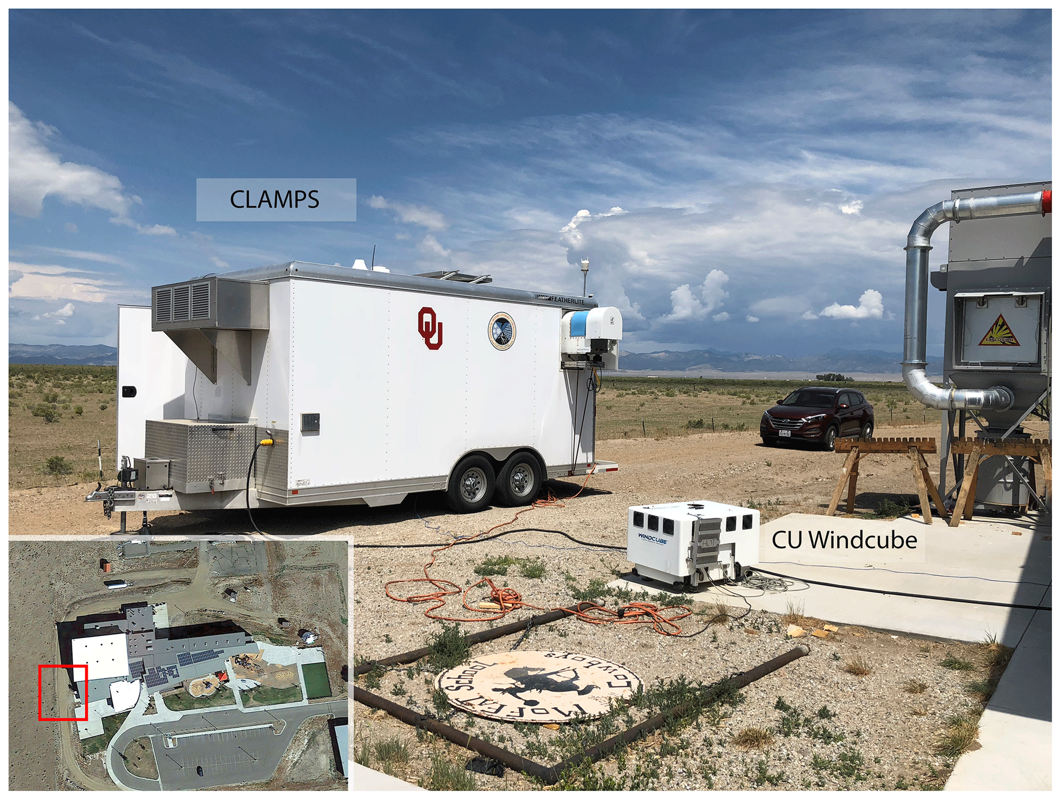
Figure 1 This photo shows the CLAMPS facility (white trailer) and the CU DPLR2 (foreground on the concrete pad) deployment location next to the Moffat Consolidated School. The red box on the satellite view shows where CLAMPS and DPLR2 were deployed in relation to the school building. Note that due to the proximity of the CLAMPS trailer to the building, the wind speed and wind direction from the meteorological station on the back of CLAMPS should be used cautiously. Satellite imagery © Google Maps.

For LAPSE-RATE, the OU DL scan strategy consisted of a 24-point plan position indicator (PPI) scan at 70^∘ elevation angle, a 6-point PPI at 45^∘, and a vertical stare. The PPIs were processed to provide horizontal wind speed and direction. The 24-point scan was chosen to try to improve the least-squares fit in complex terrain, while the 6-point scan was processed live and used as a situational awareness tool for RPAS flights. The sequence ran every 5 min, with the stare filling in the remaining time after the two PPI scans.

Finally, as part of the MWR, CLAMPS has a Vaisala WXT536 Multi-Parameter Weather Sensor mounted at a height of approximately 3 m on the back of the trailer. This weather station records air temperature, humidity, pressure, rainfall, and wind. However, the wind measurements from this campaign should be used with caution as the trailer was not optimally sited for environmental wind speed and direction measurements due to the close proximity to the Moffat Consolidated School (see Fig. 1).

Details about the processing techniques used for CLAMPS data can be found in Sect. 4.

2.2 CU Doppler lidars

In addition to the OU scanning DL, there were two profiling DLs deployed during the campaign. CU deployed a Leosphere–NRG version 1 WindCube at both the Moffat school site (Sect. 3.1, colocated with CLAMPS, Fig. 1) and at the Saguache Municipal Airport (Sect. 3.2). Hereafter, the WindCube at Moffat will be referred to as DPLR2, while the WindCube at Saguache will be referred to as DPLR1. The CU DLs were colocated at the Saguache airport for several hours from 14 July 00:04 to 21:44 UTC, at which point DPLR2 was moved to the Moffat school. The colocation allowed intercomparison between the instruments to confirm they were operating as expected.

The Doppler beam swinging (DBS) technique provides an assessment of the winds every 4 s (Lundquist et al., 2015). For the DBS technique, the version 1 WindCube (Aitken et al., 2012; Rhodes and Lundquist, 2013; Bodini et al., 2019) measures line-of-sight wind velocity along the four cardinal directions with a nominal elevation angle of 62^∘ and a temporal resolution of about 1 Hz along each beam direction (Aitken et al., 2012; Rhodes and Lundquist, 2013; Bodini et al., 2018), assuming horizontal homogeneity in the measurement volume (Lundquist et al., 2015). The measurements are taken every 20 m from 40 to 220 m a.g.l.

More info about the WindCube processing can be found in Sect. 4.

2.3 Mobile mesonet

While many of the details and specifics regarding the NSSL mobile mesonet (MM) are covered in the mobile surface observations paper in this special issue (de Boer et al., 2021), a brief description is included here for completeness. The MM concept was first introduced during the original Verification of the Origins of Rotation in Tornadoes Experiment (VORTEX) as a method of obtaining surface observations of temperature, humidity, wind speed and direction, and pressure (Straka et al., 1996).

The MM vehicle, a 2018 Ford F-250 for the LAPSE-RATE project (Fig. 2), utilizes a suite of instruments mounted on a removable equipment rack that is attached to the vehicle above the hood. This rack is mounted at a height above the roof line of the cab, such that the observations collected by the rack are as far forward and above the vehicle itself as practically possible. This is done in order to ensure that the observations are as free from influence due to the vehicle itself as possible.

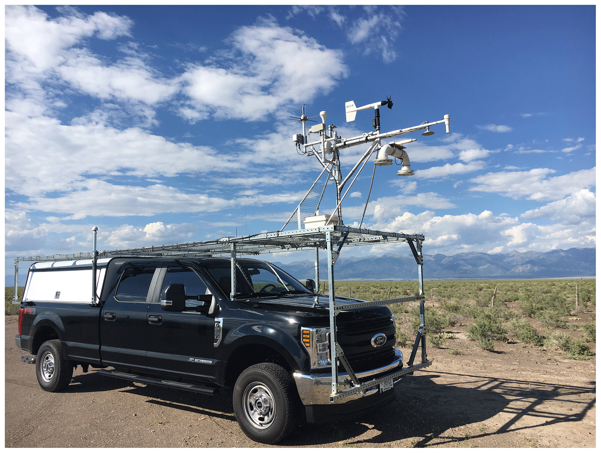
Figure 2 The NSSL mobile mesonet during the LAPSE-RATE. Photo credit Dr. Sean Waugh, NOAA/NSSL.

2.4 Radiosondes

In addition to the surface observations provided by the MM equipment rack, a Vaisala MW41 sounding system is also installed, similar to the OU CLAMPS trailer. This addition gives the MM the ability to launch radiosondes from any location in a matter of minutes and continue moving once the balloon is in the air. This advantage gives the MM the ability to launch radiosondes in rapid succession in a variety of spatial locations, which was advantageous during LAPSE-RATE due to multiple deployment locations for the RPAS teams. The bed of the F-250 holds 4 “T” tanks of helium (nominal 9.3 m³ per tank), which equates to roughly 32 potential soundings.

As previously mentioned, numerous weather balloons were launched by both the OU CLAMPS and NSSL MM deployment teams. Weather balloons have a limited spatial profile, a variable ascent path (not completely vertical), fixed sampling rates, and relatively long full profile times. These drawbacks combined with the logistical challenge and expense of launching many balloons in a relatively small area make it difficult to create high-spatiotemporal-resolution datasets from weather balloons. However despite these shortcomings, radiosondes remain the most common method of obtaining vertical profiles of temperature, humidity, wind speed and direction, and pressure. These observations are gathered routinely across the entire globe for weather forecast model initialization and are also frequently used to cross compare RPAS observations. While there are a number of manufacturers available with a variety of radiosondes to choose from, the LAPSE-RATE campaign deployed Vaisala RS92-SGP radiosondes with a Vaisala MW41 receiver. The MW41 receiver was designed for use with the newer model RS41 radiosonde but is backwards compatible with the RS92. A large supply of the slightly older RS92-SGP radiosondes was available for use during the project, hence the choice of the RS92 over the RS41. Furthermore, some of the RPASs involved with the LAPSE-RATE project used sensor configurations directly from the RS92, making this version a more suitable tool for comparison.

Table 1 RS92-SGP specifications according to the manufacturer.

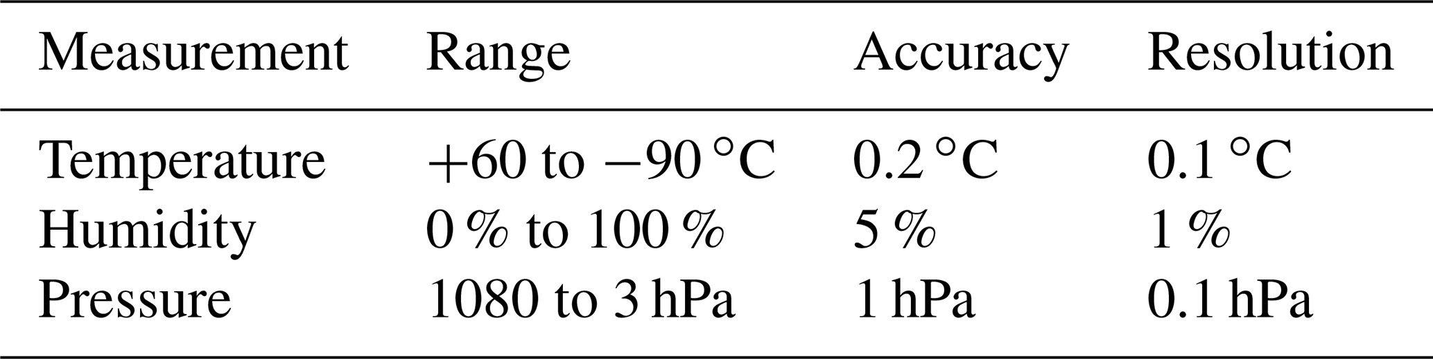
The RS92-SGP is a 400 MHz radiosonde with dual RH capacitors. The -SGP designation indicates that the radiosonde contains an internal pressure sensor as well as an onboard GPS unit. This is useful for direct observations of pressure rather than assuming a standard atmosphere. General specifications for the RS92-SGP are included in Table 1. Prior to flight, the radiosonde must be prepped for launch. This process involves connecting the RS92-SGP to the GC25 ground check station, which allows the user to set the transmission frequency. The GC25 checks the temperature sensor of the radiosonde against an internal sensor to identify bad sensors prior to launch. Though the radiosondes are shipped in sealed bags with desiccant, the RH capacitors are sensitive to aerosols and other contaminants that attach to the capacitor and can significantly bias RH observations. To remove these contaminants, the RH sensors are heated to “bake off” any foreign particles and ensure clean sensors prior to flight, maximizing accuracy of the RH profile. This is also checked against an internal desiccant chamber that should read a physical humidity of zero. If there are deviations from zero humidity, this indicates that either one or both of the RH sensors are bad, or that the desiccant in the GC25 needs to be changed. This ground check process is repeated for each radiosonde immediately prior to launch to ensure reliability and repeatability between profiles.

During flight, measurements are collected at a rate of 1 Hz and transmitted to the ground receiving station on the frequency selected. Line of sight must be maintained with the radiosonde in order to receive the data. This was a non-issue during LAPSE-RATE as the mountain valley had very little in the way of vertical winds, and no significant weather patterns were in play across the region in the upper atmosphere during the flight week. As the radiosonde ascends, the point-to-point GPS observations are collected and filtered to produce horizontal winds.

For the RH observations, measurements are taken from a single RH chip while the other is heated for a period of approximately 10 s. This sensor is then allowed to cool, and the observations are switched to the second sensor while the first is heated. This process is repeated throughout the entire flight. As the radiosonde ascends, particularly through the boundary layer, the RH capacitors will encounter aerosols and other contaminants that can bias the RH observations similar to those removed prior to launch by the GC25. The alternative heating process removes these contaminants continuously during data collection and also eliminates sensor icing on the RH sensors. As the radiosonde ascends, solar radiative forcing becomes a more significant influence on the observed air temperature as the sensor is heated due to sunlight. To remove this effect, an offset is applied by the MW41 software to the observed temperature to correct for the solar heating. This correction is applied based on location and time of day to take into account solar angle.

3 Measurement locations

A plan view of the San Luis Valley of Colorado is included in the introduction paper to this special issue (see Fig. 1 in de Boer et al., 2020b). A simplified map with locations relevant to this paper is shown in Fig. 3. In addition to fixed locations, the launch points of all the radiosondes launched by the MM are shown. While the majority of the NSSL MM radiosondes were launched at Leach Airfield, some mobile radiosondes were launched near the Saguache Municipal Airport near the end of the flight campaign. This was done in support of a move to make RPAS observations by a few teams on a more mobile scale. The fixed locations are discussed in more detail in the following sections.

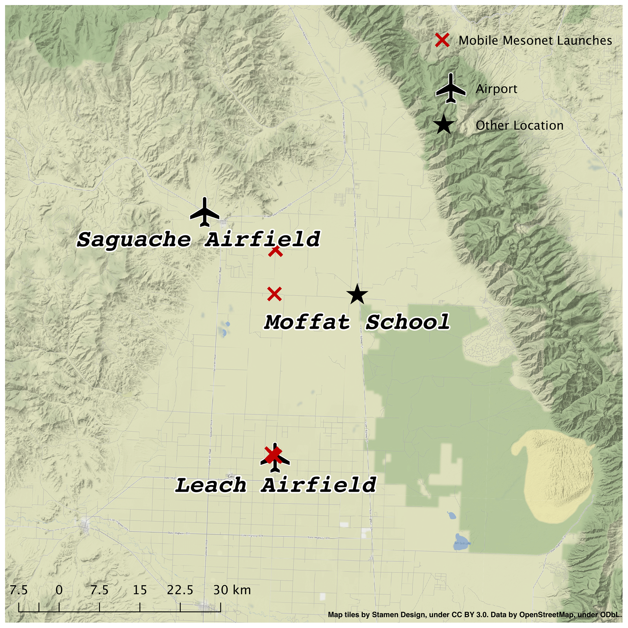
Figure 3 Sounding locations for the NSSL mobile vehicle (red X's) and locations of profiling systems during LAPSE-RATE. The OU CLAMPS trailer performed all of their soundings at the Moffat school site. © OpenStreetMap contributors 2020. Distributed under a Creative Commons BY-SA License.

3.1 Moffat Consolidated School

During LAPSE-RATE, CLAMPS and DPLR2 were deployed at the Moffat Consolidated School in Moffat, CO. The location of Moffat in the valley was advantageous as it was centered between the mountain ranges to the east and west. CLAMPS and the CU DL could therefore act to provide data on the background flow and thermodynamics, while the RPASs scattered throughout the valley were able to provide hyper-local observations more sensitive to the varying boundary layer conditions affected by the terrain. Additionally, the Moffat site could fulfill the power requirements of CLAMPS and provide a flat place to deploy the trailer. Finally, the school staff were extremely accommodating in allowing access to their internet connection, which allowed for improved communications with other teams and data retrieval.

3.2 Saguache Municipal Airport

DPLR1 was deployed at the Saguache Municipal Airport in the northwest corner of the valley. The airport is located at the mouth of a small valley leading down out of the mountains, which provides an ideal location for sampling drainage flow induced by the terrain. The Automated Weather Observing System (AWOS) at the airport (K04V) often observes this nocturnal drainage flow, which is one of the phenomena targeted for observation by RPASs. DPLR1 was colocated with weather observing RPASs from OU (Pillar-Little et al., 2021).

3.3 Leach Airfield

Leach Airfield served as a central focus point to many of the operations scattered throughout the valley during the flight week. Being centrally located, it provided a relatively stable set of kinematic and thermodynamic conditions with minimal direct influence of terrain induced flow and is located over a portion of the valley that is exceptionally flat. With these conditions, the airfield served as a proving ground of sorts for the RPASs to conduct calibration flights against other RPASs (Barbieri et al., 2019), the MURC vehicle from CU (de Boer et al., 2020b), the surface observations from the NSSL MM, and various radiosonde launches by the NSSL MM. During the flight week, teams were allowed complete access to the field surrounding the runway at Leach Airfield, which was largely non-irrigated (though nearby fields were), with short patchy grass and dirt as is evident in Fig. 4.

Figure 4 A radiosonde launch at Leach Airfield by Dr. Sean Waugh. Photo credit Dr. Sean Waugh, NOAA/NSSL.

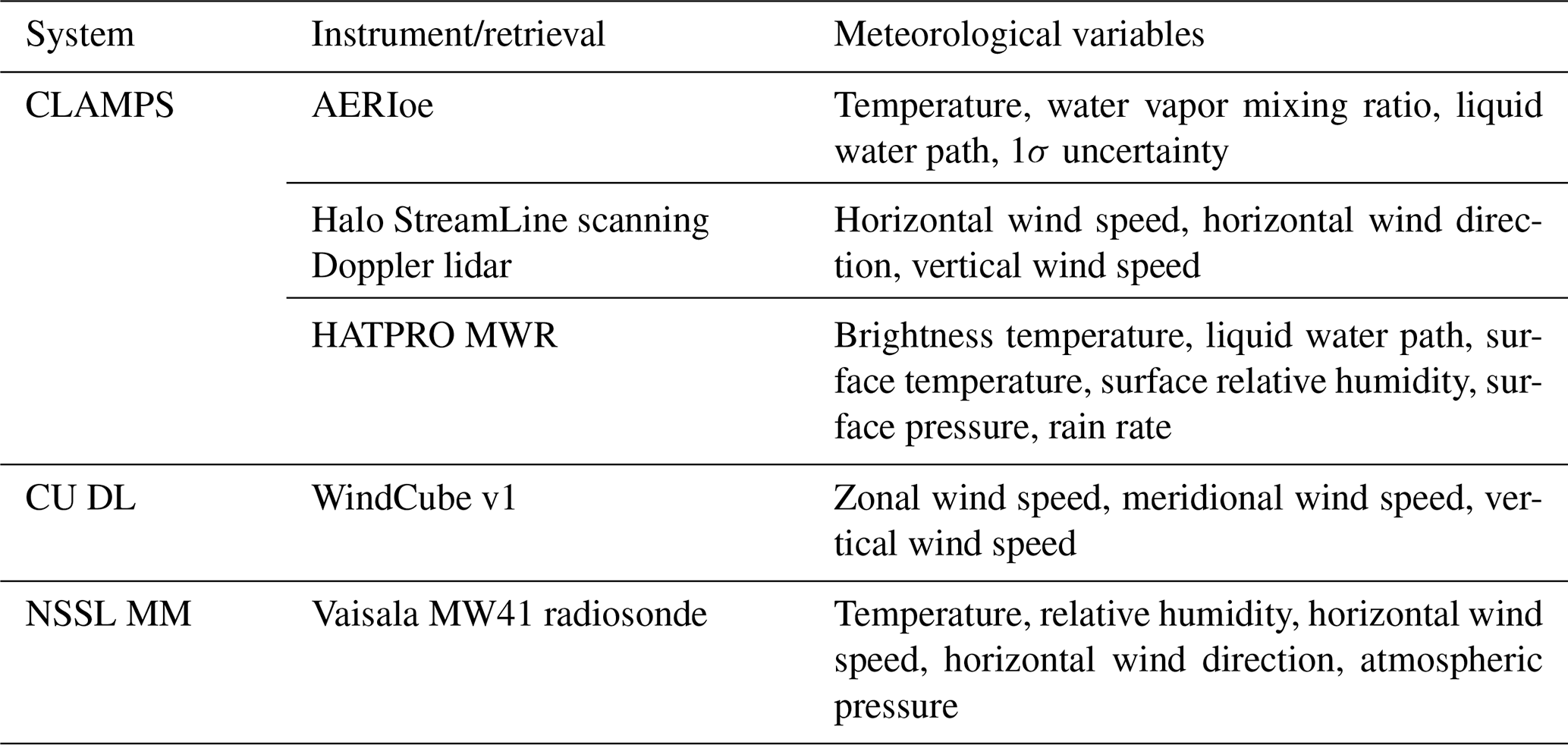
Table 2 A list of the systems described in the paper with details about the instruments/retrievals provided by each system. Additionally, the major meteorological variables produced by each instrument/system are included.

4 Data processing

Each of the datasets presented in this article are the result of careful processing and quality control (QC) to ensure that the data are as free from error and as easy to interpret as possible. This process produces a series of data levels from raw data to some final product that incorporates error and bias correction and QC processes. The general guidelines for the file structure are discussed in de Boer et al. (2020b). Presented here are the specific processing steps and QC flags applied to the data collected by the systems described in Sect. 2.

4.1 CLAMPS

The AERI and MWR in CLAMPS were combined in a joint thermodynamic retrieval using the AERI optimal estimation technique (AERIoe,  Turner and Löhnert, 2014; Turner and Blumberg, 2018). Specifically, AERIoe version 2.8 was used. This retrieval is a physical iterative retrieval that attempts to convert radiance and brightness temperature observations to temperature and moisture profiles. However, the retrieval is an ill-posed problem; there are many possible solutions. Thus, this retrieval requires a prior and first guess in order to operate successfully. The prior dataset used was produced from radiosondes launched from the National Weather Service in Boulder, Colorado. This is not an ideal prior, as the climatological conditions in Boulder do not fully represent the conditions in the San Luis Valley. Due to this, additional data were also included in the AERIoe retrieval to try and further constrain the solution. These included surface temperature and relative humidity from the CLAMPS Vaisala WXT-530, radiosondes launched from CLAMPS (used to constrain above 3 km), and the CLAMPS Doppler lidar backscatter (used to detect cloud base). Although the MWR was calibrated at the beginning of the campaign, the brightness temperatures input into AERIoe from the MWR were bias corrected using the colocated radiosondes. The AERIoe data were processed at 15 min resolution to match the cadence of the colocated WxUAS profiles (Pillar-Little et al., 2021). The vertical resolution decreases exponentially with height, starting at 10 s of meters at the surface and decreasing to approximately 100 m at 1 km a.g.l.

The AERIoe files are provided in netCDF format. Each file contains thermodynamic variables (temperature, water vapor mixing ratio, etc.). Additionally, some radiative products are also included in the netCDF file (e.g., liquid water path, liquid water effective radius). All retrieved variables have a 1σ uncertainty that is produced by the algorithm. For more information on the retrieval itself, see Turner and Löhnert (2014) and Turner and Blumberg (2018) for an overview.

The Doppler lidar PPI scan files were post-processed using the velocity–azimuth display (VAD) technique (Browning and Wexler, 1968). In order to minimize the impact of spatial heterogeneities, only the 70^∘ PPI scan was used to calculate the VAD. The VAD technique produces estimates of the horizontal wind speed and direction. The Doppler lidar data are provided in three different netCDF files: one containing the stare data (DLFP), one containing the PPI data (DLPPI), and the last containing the processed VAD data (DLVAD). These files are provided in netCDF format.

4.2 CU DL

The CU DL data are provided in netCDF format. The file contains measurements of the wind at 1 s temporal resolution at 10 heights, ranging from 40 to 220 m. The estimates of zonal (u), meridional (v), and vertical (w) winds rely on the DBS technique (Lundquist et al., 2015), assuming horizontal homogeneity over the measurement volume. Each beam has a carrier-to-noise ratio (CNR) value returned for each measurement height, and all data with CNR values less than −27 dB are neglected.

These DLs were colocated at Saguache from 14 July 2018 00:04 UTC to 14 July 2018 21:44 UTC. When correlating data from this time period, it was discovered that the timestamp on DPLR2 was approximately 20 min ahead of DPLR1. This offset error has been corrected in the netCDF files. More information about the processing as well as validation can be found in Rhodes and Lundquist (2013) and Lundquist et al. (2015). In addition to measurements of winds and derived quantities like turbulence intensity and turbulence kinetic energy, these lidar data allow estimation of the turbulence dissipation rate (Bodini et al., 2019).

4.3 Radiosondes

The MW41 sounding system automatically produces a series of files that contain the relevant profile information as well as information regarding the time of launch, radiosonde used, launch location, etc. These files contain the raw (i.e., uncorrected) pressure, temperature, and humidity data; the raw GPS coordinates of each data record; and the Vaisala proprietary filtered products. Rather than tracking multiple files for each deployment, the files are first collected and combined into a single large data record. Timing information is included in each file, which makes aligning data points straightforward. The first main record of this combined file is the surface conditions that were input by the user during operations, while the entirety of the ascent portion of the sounding is contained in the records that follow (the sounding is terminated when the descent portion of the profile begins following the balloon burst).

In addition to the sounding records themselves, a number of profile-based parameters are also calculated and included for reference (Table 3). Furthermore a quality control flag of logic value 0 (false) or 1 (true) indicates if the sounding reached a minimum profile height of 300 hPa. These parameters are common to radiosonde data presentation and are well known/documented. For more information on the specifics of these parameters, readers are encouraged to reference the AMS Glossary (https://glossary.ametsoc.org/wiki/Welcome, last access: 11 March 2021).

Table 3 A list of sounding parameters that are calculated and available in the radiosonde files. Variables marked with an asterisk were calculated for surface based, most unstable, and the lowest 100 hPa mixed parcels. “LR” denotes “lapse rate”, while “WS” denotes “wind shear”.

Regarding the full data records themselves, there are a number of groups of variables that deserve direct discussion. The filtered data in the file contain the Vaisala specific filters mentioned previously. The wind algorithm filter is meant to remove the pendulum oscillations that are common with balloon launched devices and generally smooth the data. It should be noted that this wind algorithm is proprietary, and as such the derived winds from the automated MW41 sounding system are somewhat of a “black box” and should be treated with caution. This data group also contains the solar radiation corrected temperature as mentioned earlier. The Vaisala filtered u and v wind components and a computed mixing ratio are also contained here.

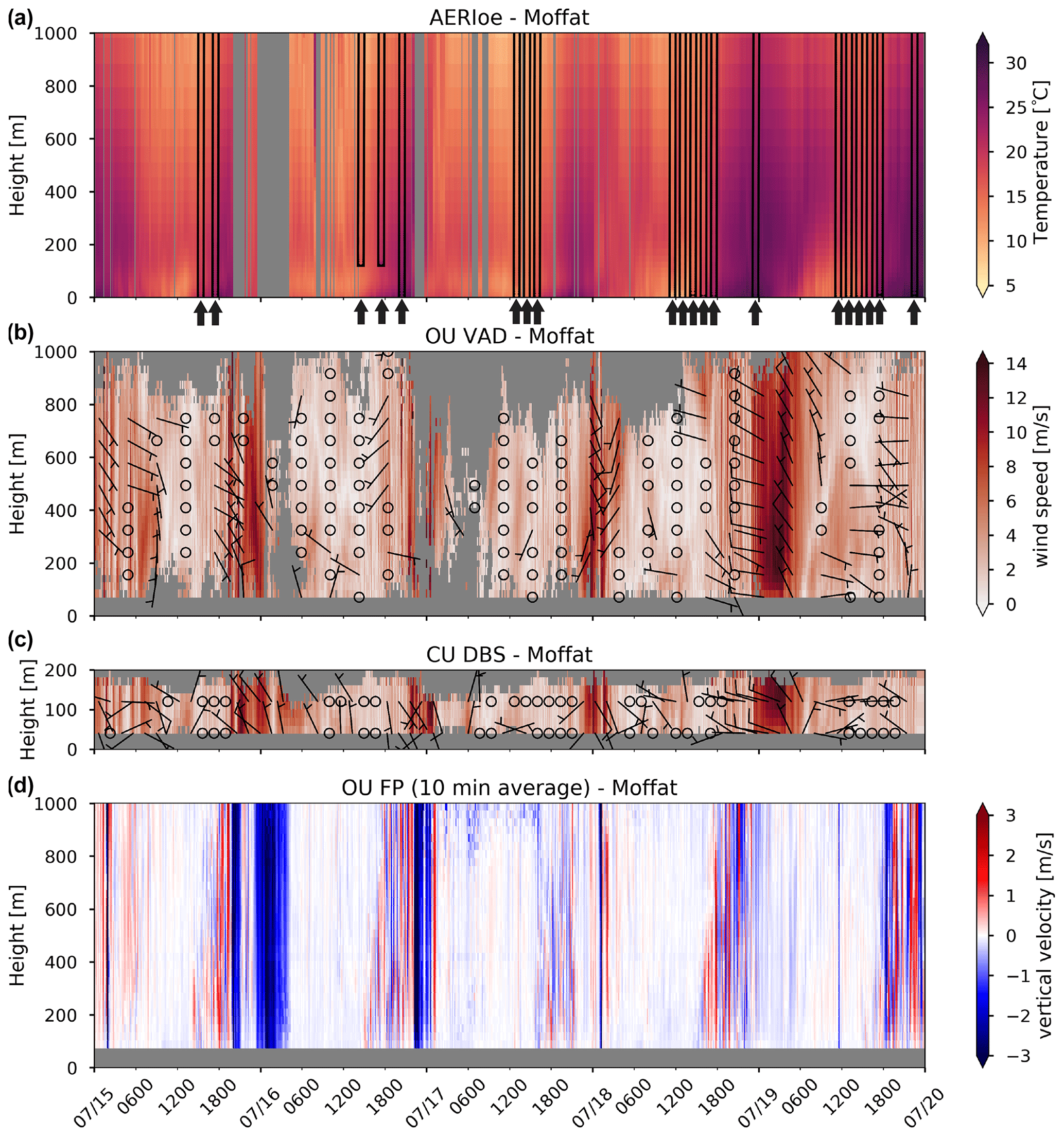
Figure 5 Time–height figures of temperature from the AERIoe retrievals (a), wind speed and direction from the CLAMPS VAD (b), wind speed and direction from the CU DBS scan (c), and 10 min averages of the vertical velocity measured from the CLAMPS vertical stare (d) from the full LAPSE-RATE campaign. All of these data were recorded at the Moffat site. Radiosonde data are overlaid and outlined in black on top of the AERIoe retrievals in panel (a). The launch time of each radiosonde in indicated with a black arrow.

As a counterpart to the filtered data section, there is a raw data section which contains unprocessed information directly off the radiosonde. This includes the raw point-to-point GPS coordinates and the uncorrected pressure, humidity, and temperature data. This information can be useful in specific situations or if attempting to work with data without the proprietary filter applied. This section also includes manually derived winds from the raw GPS coordinates. This was done using point-to-point differences between successive GPS locations, with no smoothing or filtering of any kind to provide a clean wind record that could be filtered by the end user. This process inherently averages any accelerations of the balloon over a given 1 s period as it is only looking at the horizontal motion between two successive points. Additionally it is also assumed that the balloon is moving entirely with the wind and has no deviant motion of its own. Therefore taking the distance traveled by the balloon in a known period of time, the horizontal winds may be calculated at that point in space and time.

5 Sample data

In this section, sample data are shown from each profiling platform discussed in Sect. 2. Figure 5 showcases data from the Moffat site where radiosondes, CLAMPS, and a CU DL were colocated for the experiment. This provides opportunity to see how the various platforms compare in space and time as well as quality and availability.

Figure 5a shows data from both the CLAMPS AERIoe temperature retrieval and the temperature recorded from the colocated radiosonde launches, which are the colored lines overlaid on top. The grey areas indicate one of two things: either the retrieval did not converge or it was raining during this period, and thus there is no valid data. During the campaign, very short lived rain showers would often form sporadically throughout the day, hence the short periods of data drops.

Wind speed and direction from the CLAMPS DL is shown in Fig. 5b. Similar to Fig. 5a, grey areas in this figure show when rain was present. In addition, grey areas could signify that a good VAD fit was not achieved. The latter most often happens during strong daytime heating, where strong updrafts were common. A detailed intercomparison of the CLAMPS facility data, the Moffat radiosonde data, and data from the colocated weather-sensing RPASs can be found in Bell et al. (2020c).

In total, there were 25 radiosonde launches from the NSSL MM, with 20 of those from Leach Airfield and 5 from near Saguache. The time and location of the radiosonde launch depended on the specific mission goals that day (e.g., morning transition, drainage flow, convection). A full description of the science goals for each day is provided in de Boer et al. (2020b). Rather than show all available datasets, a focus of available data from the final day of the project near Saguache is presented. All five soundings rose entirely through the troposphere, with an average maximum altitude of 21 km a.g.l. The simplest way to visualize a single sounding is using programs such as SHARPpy (Blumberg et al., 2017) or MetPy (May et al., 2008–2020). Figure 6 shows an example Skew-T diagram created using MetPy.

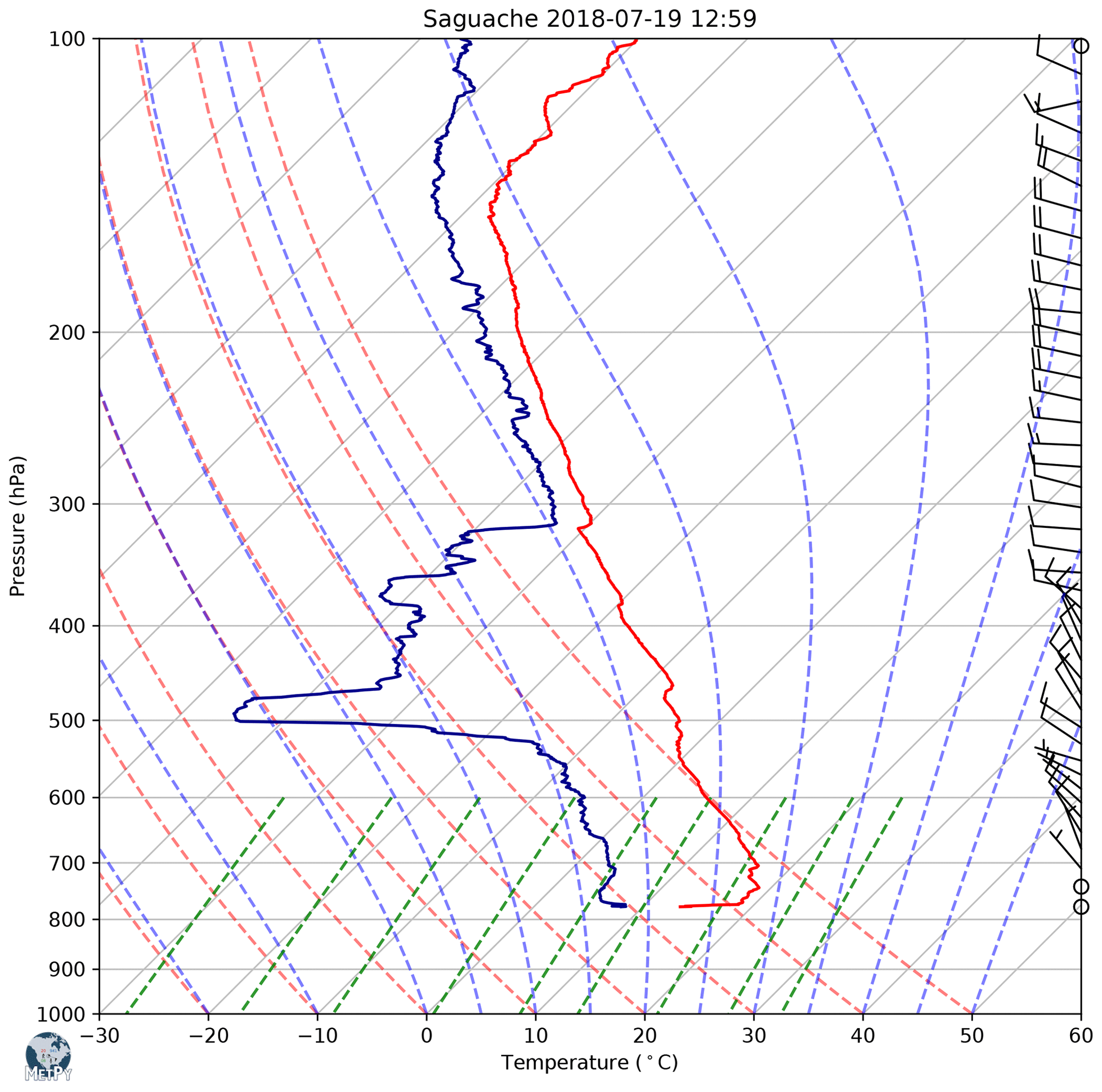
Figure 6 Sounding launched from near Saguache, CO, at 12:59 UTC. Image created using MetPy (May et al., 2008–2020).

The sounding shows a dry profile through a depth of nearly 7 km a.g.l. before high level clouds were encountered. Near the surface, a super adiabatic layer exists, marking the sharp inversion immediately above the somewhat moist nocturnal mountain boundary layer. Sharp inversions such as this were common during flight week, particularly with the calm winds in the lowest 1 km. Many of the launches saw very weak or non-existent wind profiles until the radiosonde rose above the rim of the mountains surrounding the valley.

In addition to examining individual soundings, which can be useful for more direct comparisons with RPASs, we can also look at deployment days in a more holistic sense through a time series analysis (Fig. 7). Examining the data in this way highlights the stably stratified layers near the surface in the early morning hours with the mountain boundary layer. Starting around 15:00 UTC, as the sun rises over the valley the radiosondes were able to capture the transition to the deeper, more convective daytime boundary layer. Similar profiles and time history plots can be made using RPAS data to compare the ability of an RPASs to reproduce observed profiles obtained from standard instruments.

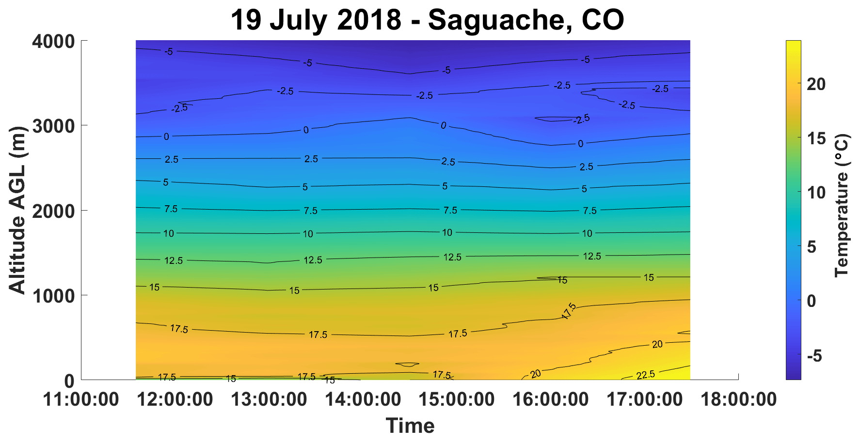
Figure 7 Time series of air temperature from five radiosondes launched near Saguache. Sounding times were 11:35, 12:59, 14:30, 16:00, and 17:29 UTC. Temperature values between sounding times are interpolated.

6 Data availability

The data in this paper are all publicly available on the data hosting website Zenodo. The references for each dataset are as follows: CLAMPS Doppler lidar (https://doi.org/10.5281/zenodo.3780623; Bell and Klein, 2020), CLAMPS MWR and surface observations (https://doi.org/10.5281/zenodo.3780593; Bell et al., 2020b), AERIoe retrievals (https://doi.org/10.5281/zenodo.3727224; Bell et al., 2020a), mobile mesonet radiosonde (https://doi.org/10.5281/zenodo.3738175; Waugh, 2020b), CLAMPS radiosondes (https://doi.org/10.5281/zenodo.3720444; Waugh, 2020a), and CU Doppler lidar (https://doi.org/10.5281/zenodo.3698228 Lundquist et al., 2020).

7 Summary

In order to fulfill the need for more observations of the ABL, a large group of scientists deployed multiple types of boundary-layer profiling systems in the San Luis Valley in southern Colorado to evaluate the current capabilities of these systems. These instruments include weather-sensing RPASs, ground-based remote sensors, and radiosondes. While a large part of the campaign was devoted to using weather-sensing RPASs, the more established remote sensors and radiosondes provided the background state of the atmosphere and augmented the RPAS observations. Radiosondes were launched from the NSSL MM around the valley depending on the weather conditions being studied. Additionally, radiosondes were launched from the CLAMPS system at the Moffat site, which was centrally located in the valley. Finally, CU deployed two Doppler lidars in the valley: one at the Moffat site and one at the Saguache municipal airport. This paper gives an overview of all these instruments, the conditions they sampled, and a brief description of the file formats.