European anthropogenic AFOLU greenhouse gas emissions: a review and benchmark data

Emission of greenhouse gases (GHGs) and removals from land, including both anthropogenic and natural fluxes, require reliable quantification, including estimates of uncertainties, to support credible mitigation action under the Paris Agreement. This study provides a state-of-the-art scientific overview of bottom-up anthropogenic emissions data from agriculture, forestry and other land use (AFOLU) in the European Union (EU28¹). The data integrate recent AFOLU emission inventories with ecosystem data and land carbon models and summarize GHG emissions and removals over the period 1990–2016. This compilation of bottom-up estimates of the AFOLU GHG emissions of European national greenhouse gas inventories (NGHGIs), with those of land carbon models and observation-based estimates of large-scale GHG fluxes, aims at improving the overall estimates of the GHG balance in Europe with respect to land GHG emissions and removals. Whenever available, we present uncertainties, its propagation and role in the comparison of different estimates. While NGHGI data for the EU28 provide consistent quantification of uncertainty following the established IPCC Guidelines, uncertainty in the estimates produced with other methods needs to account for both within model uncertainty and the spread from different model results. The largest inconsistencies between EU28 estimates are mainly due to different sources of data related to human activity, referred to here as activity data (AD) and methodologies (tiers) used for calculating emissions and removals from AFOLU sectors. The referenced datasets related to figures are visualized at https://doi.org/10.5281/zenodo.3662371 (Petrescu et al., 2020).

1 Introduction

The atmospheric concentrations of the main greenhouse gases (GHGs) have increased significantly since preindustrial times (pre-1750), by 46 % for carbon dioxide (CO₂), 257 % for methane (CH₄) and 122 % for nitrous oxide (N₂O) (WMO, 2019). The rise of CO₂ levels is caused primarily by fossil fuel combustion, with a substantial contributions from land use change. Increases in emissions of CH₄ are mainly driven by agriculture and by fossil fuel extraction activities, while increases in natural emissions post-2006 cannot be ruled out (e.g., Worden et al., 2017). Increases in N₂O emissions are largely due to anthropogenic activities, mainly in relation to the application of nitrogen (N) fertilizers in agriculture (FAO, 2015; IPCC, 2019b). Globally, fossil fuel emissions grew at a rate of 1.5 % yr⁻¹ for the decade 2008–2017 and account for 87 % of the anthropogenic sources in the total carbon budget (Le Quéré et al., 2018b). In contrast, global emissions from land use change were estimated from bookkeeping models and land carbon models (dynamic global vegetation models, DGVMs) to be approximately stable in the same period, albeit with large uncertainties (Le Quéré et al., 2018b). Importantly, emissions arising from land management changes were not estimated in the global carbon budget.

National greenhouse gas inventories (NGHGIs) are prepared and reported by countries based on IPCC Guidelines (GLs) using national data and different calculation methods (tiers) for well-defined sectors. The IPCC tiers represent the level of sophistication used to estimate emissions, with Tier 1 based on default assumptions, Tier 2 similar to Tier 1 but based on country-specific parameters, and Tier 3 based on the most detailed process-level estimates (i.e., models).

After 2020, European countries will report their GHG emission reductions following the newly approved UNFCCC transparency framework (UNFCCC, 2018), including the reporting principles of transparency, accuracy, consistency, completeness and comparability (TACCC), as well as using the IPCC methodological guidance (IPCC Guidelines, 2006). Furthermore, the IPCC 2019 Refinement (IPCC, 2019a) (that may be used to complement the 2006 IPCC GLs) has updated guidance on the possible and voluntary use of atmospheric data for independent verification of GHG inventories. So far, only few countries (e.g., Switzerland, UK and Australia) are already using atmospheric GHG measurements, on a voluntary basis, as an additional consistency check of their national inventories. Annex I² countries (including the EU) submit annually complete inventories of GHG emissions from the 1990 base year³ until 2 years before the current reported year, and these inventories are all reviewed to ensure TACCC. This allows for most of these Annex I countries to track progress towards their reduction targets committed for the Kyoto Protocol (UNFCCC, 1997) and now for the Paris Agreement (PA) (United Nations, 2015).

According to UNFCCC (2018) NGHGI estimates, the European Union (EU28) in 2016 emitted 3.9 Gt of CO₂ equivalents (CO₂ eq.) (including LULUCF/FOLU⁴) and 4.2 Gt CO₂ eq. (excluding LULUCF) (the GWP100 metric⁵, IPCC, 2007, is here used to compare different gases in CO₂ eq.). These anthropogenic emissions, including LULUCF, represent about 8 % of the world total. This number is consistent with the EDGAR v4.3.2FT2017 inventory (Olivier and Peters, 2018) using IEA (2017) and BP (2018) data for energy sectors and EDGARv4.3.2 (Janssens-Maenhout et al., 2019) and FAOSTAT (2018) for other (mainly agricultural and land use) sectors. A few large economies accounted for the largest share of EU28 emissions, with UK and Germany representing 33 % of the total EU28 emissions.

Figure 1 Total reported EU28 GHG emissions according to UNFCCC NGHGI (2018) data. Remaining land refers to CO₂ emissions from the LULUCF sector belonging to all six management classes (forest land, cropland, grassland, wetlands, settlements and other land). The IPCC good practice guidance (GPG) for land use, land use change and forestry (IPCC, 2003) describes a uniform structure for reporting emissions and removals of GHGs. This format for reporting can be seen as land based; all land in the country must be identified as having remained in one of six classes since a previous survey or as having converted to a different (identified) class in that period. According to 2006 IPCC GLs, land should be reported in a “conversion” category for 20 years and then moved to a “remaining” category, unless a further change occurs. Data belonging to the six management classes are found in the EU CRF Table 4 (European Union CRF (Convention) accessible at https://unfccc.int/process-and-meetings/transparency-and-reporting/reporting-and-review-under-the-convention/greenhouse-gas-inventories-annex-i-parties/submissions/national-inventory-submissions-2018, last access: February 2020.), points 4.A.1, 4.B.1, 4.C.1, 4.D.1, 4.E.1 and 4.F.1. Converted land refers to CO₂ emissions from conversions to and from all six classes that occurred in the previous 20 years, as reported in the NGHGI (2018) submissions EU CRF Table 4, points 4.A.2, 4.B.2, 4.C.2, 4.D.2, 4.E.2 and 4.F.2. Harvested wood products (HWPs) are reported in the NGHGI (2018) submissions EU CRF Table 4, point 4.G. Bioenergy emissions are reported as a memo item under the energy sector (EU CRF Table 1s2). These emissions are reported as a decrease in carbon stock change in the LULUCF sector and thus by convention not accounted for in the energy sector.

According to NGHGI 2018 data, total anthropogenic emission of GHGs in the EU28 (Fig. 1) decreased by 24 % from 1990 to 2016 (UNFCCC, 2018). CO₂ emissions (including LULUCF) account for 81 % of the total EU28 emissions in 2016 and declined 24 % since 1990, accounting for 71 % of the total reduction in GHG emissions. CH₄ emissions account for 10 % of and N₂O emissions account for 19 % of total GHG emissions; both gases have had a reduction of 37 % from 1990 levels. These reductions were due to both European and country-specific policies on agriculture and the environment implemented in the early 1990s (e.g., the nitrogen directive which limited the amount of N use in agriculture with repercussions for both fertilizer use and livestock numbers) and energy policies in the 2000s, (e.g., the EU Emissions Trading System, ETS; and support for renewable energy and energy efficiency). The specific policies triggered lower levels of mining activities, smaller livestock numbers, and lower emissions from managed waste disposal on land and from agricultural soils. Specific historical structural changes in the economy linked to the collapse of eastern European economies in early 1990s, the discovery and development of large natural gas sources in the North Sea, and more recently the economic recession in 2009–2012, contributed as well to these diminishing trends (Karstensen et al., 2018). A few large, populous countries account for the largest share of EU28 emissions (UK and Germany combined represent 33 % of the total), while the reduction of total emissions in 2016 compared to 1990 is led by UK (38 %), Germany (24 %), Spain (23 %), Poland (18 %), Italy (15 %) and France (11 %) (Olivier and Peters, 2018).

Emissions from LULUCF represented in 2016 a sink of about 300 Mt CO₂, and this sink has increased 15 % from 1990 to 2016. Bioenergy emissions are reported as a memo in the energy sector, as the emissions are captured already under LULUCF.

For CH₄, the two largest anthropogenic sources in the EU28 are the agriculture (e.g., emissions from enteric fermentation) and waste (e.g., anaerobic waste) sectors. These two sources accounted for 90 % of total EU28 CH₄ emissions in 2016 excluding LULUCF (EEA, 2018), with agriculture accounting for 53 % of total EU28 CH₄ emissions in 2016 excluding LULUCF, that is, 11 % of total EU28 GHG emissions excluding LULUCF in 2016. We exclude CH₄ emissions from LULUCF because they only represent 1.5 % of total EU28 CH₄ emissions in 2016. From 1990 to 2016, the total CH₄ emissions from EU28 decreased by 31 % (554 Mt CO₂ eq.). The top five EU28 emitters of CH₄ are France (13 %), Germany (12 %), UK (12 %), Poland (11 %) and Italy (10 %), which account for 56 % of total EU28 CH₄ emissions (excluding the LULUCF sector).

For N₂O, the largest EU28 sources are agriculture and the industrial processes and product use (IPPU) sectors, while the FOLU subsectors that cover emissions from forests are a small N₂O source. Agriculture contributes emissions largely from the use of fertilizers in agricultural soils, while industrial production of nitric and adipic acid dominates IPPU-related emissions. These sources accounted for 85 % of N₂O emissions in 2016, that is, 5 % of total EU28 GHG emissions estimates in 2016. From 1990 to 2016, the total N₂O emissions decreased by 35 % (251 Mt CO₂ eq.). The top five EU28 emitters of N₂O are France (18 %), Germany (16 %), UK (9 %), Poland (8 %) and Italy (8 %), which account for 59 % of the total N₂O EU28 emissions (excluding the LULUCF sector).

Zooming in on trends, non-CO₂ emissions show a very small decrease (−0.4 %) from 2004 to 2014 and an increase (+0.8 %) from 2015 to 2017 (Olivier and Peters, 2018). This recent growth is principally determined by the increase in N₂O emissions which have offset the declining CH₄ emissions. The continued CH₄ emissions decrease is mainly due to shifts in the fossil fuel production from coal to natural gas in Germany, Italy and the Netherlands (BP, 2018).

The main objective of the present study is to present a synthesis of AFOLU GHG emission estimates from bottom-up approaches that can serve as a benchmark for future assessments, which is important during the reconciliation process with top-down GHG emission estimates. We use existing officially reported data from NGHGI submitted under the UNFCCC as well as other emission estimates based on research data, from global emissions datasets to detailed biogeochemical models. The bottom-up approaches considered, although based on independent efforts from those in the NGHGI, have some level of redundancy among them and the inventories, since they often use similar activity data (AD) and largely apply the current IPCC (2006) methodology, albeit using different tiers.

Independent bottom-up estimates are valuable to compare with estimates officially reported to the UNFCCC and may identify differences that need closer investigation. The uncertainties presented in this paper are taken from the UNFCCC NGHGI (2018) submissions. For the global emissions dataset EDGAR uncertainties are only calculated for the year 2012 as described in the Appendix B. We evaluate the reason for differences in emissions by carefully comparing the estimates, quantifying uncertainties and detecting discrepancies. We compare the inconsistencies (defined by differences between estimates) to the uncertainties (error associated with each estimate) and identify those sectors that would yield the most benefit from improvements. Uncertainties from the other datasets and models were not yet available. We do include natural CH₄ emissions from wetlands, whose accounting will become mandatory from 2026 under the new EU LULUCF Regulation (https://eur-lex.europa.eu/legal-content/EN/TXT/?uri=uriserv:OJ.L_.2018.156.01.0001.01.ENG&toc=OJ:L:2018:156:FULL, last access: October 2019).

2 Compilation of AFOLU emission estimates

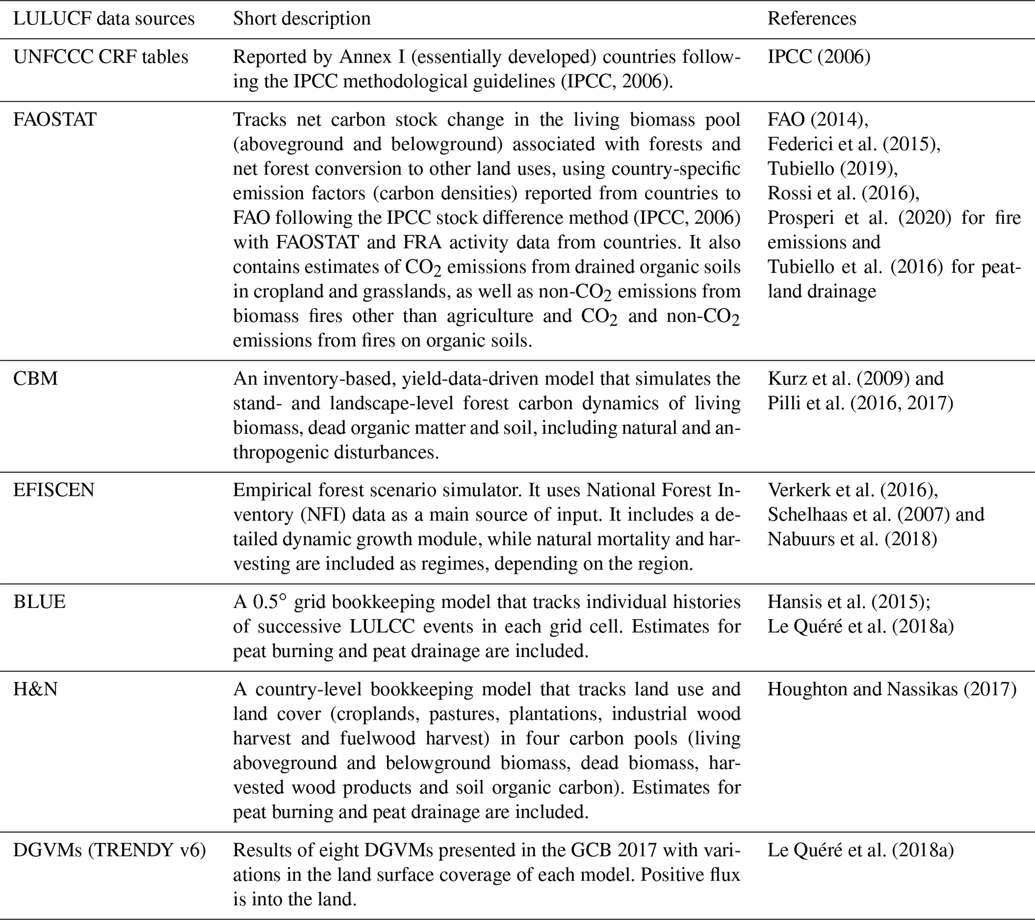
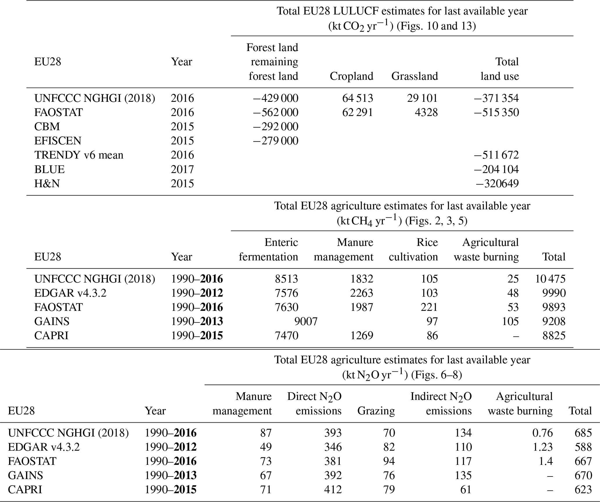
We collected available data of AFOLU emissions and removals (Table 1) between 1990 and 2016 (or last available year) that have been documented in peer-reviewed literature. The collection of data represents the latest data available and most recent state of the art of available estimates of GHGs representing the AFOLU sector in Europe as derived from our knowledge of the scientific literature and the scientific networks in Europe. UNFCCC NGHGI and other data sources for AFOLU emissions or component fluxes as well as methodologies are described in Appendix B. For all three GHGs, total emissions from agriculture and LULUCF for the EU28 are presented in Appendix Table A2.

Whenever necessary we provide details on individual countries separating CO₂, CH₄ and N₂O. The units are based on the metric ton (t) (1 kt = 10⁹ g; 1 Mt = 10¹² g) for individual gases and (Mt =10¹² g; 1 Tg = 10¹² g) for CO₂ and carbon (C) from AFOLU sectors. We rely on modeled and reported data streams to quantify GHG fluxes from bottom-up models together with country-specific inventory from NGHGI official statistics (UNFCCC), global inventory datasets (EDGAR), global statistics (FAOSTAT) and global land GHG biogeochemical models used for research assessments (e.g., DGVMs, bookkeeping models). The values in this study are defined from an atmospheric perspective, which means that positive values represent a source to the atmosphere and negative ones a removal from the atmosphere.

Table 1 Summary of AFOLU data sources for the three main GHGs available and their references. The last reported year for each underlying database used in this study is highlighted in bold.

As an overview of potential uncertainty sources, Tables A1a and b present the use of emission factor data (EF), activity data (AD), and, whenever available, uncertainty estimation methods used for all agriculture and forestry data sources used in this study. The referenced data used for the figures' replicability purposes are available for download at https://doi.org/10.5281/zenodo.3662371 (Petrescu et al., 2020). The complete emissions data can be found and downloaded from the source websites, as described in Appendix A, Table A1a and b.

3 Emission estimates

As part of the AFOLU sectors, agricultural activities play a significant role in non-CO₂ GHG emissions (IPCC, 2019b; FAO, 2015). The two major gases emitted by the agricultural sector are CH₄ and N₂O. According to the 2018 UNFCCC NGHGI data updated up to the year 2016, agriculture contributes as much as 11 % from the total EU28 GHG emissions expressed in CO₂ equivalents (year 2016, UNFCCC NGHGI, 2018). In 2016, CH₄ from agricultural activities accounted for 53 % of total EU28 CH₄ emissions, while N₂O accounted for 78 % of N₂O emissions. The preponderant share of agriculture in total anthropogenic non-CO₂ emissions also applies globally (IPCC, 2019b). The CO₂ emissions reported as part of the agriculture sector only cover the liming and urea application, IPCC sectors 3G and 3H respectively. In terms of CO₂ they only represent < 5 % of the total GHG emissions from agriculture and are therefore not included in this study.

Regarding the forestry subsector of AFOLU, LULUCF, the major GHG gas is CO₂. According to UNFCCC NGHGI (2018) data, in 2016, the total EU28 LULUCF sector was a net CO₂ sink of 314 Mt CO₂. We note that in general the reported values for GHG emissions do not include the flux estimates from LULUCF, which are usually accounted for separately, because they are inherently very uncertain and show large interannual variations as a result of interannual variability in climatic conditions and (in part as a consequence of this variability) in natural disturbances (Kurz et al., 2010; Olivier et al., 2017).

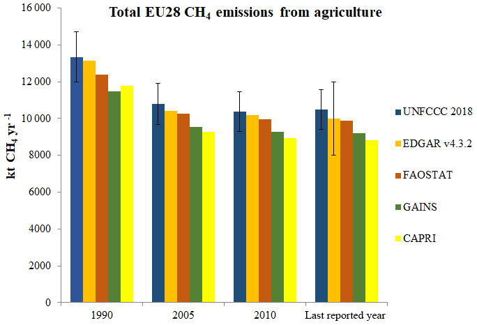
Figure 2 Total EU28 agriculture CH₄ emissions from five data sources: UNFCCC NGHGI (2018) submissions, EDGAR, FAOSTAT, CAPRI and GAINS. The relative error on the UNFCCC value, computed with the 95 % confidence interval method, is 10 %. It represents the NGHGI 2018 uncertainty for the agriculture data reported to UNFCCC. Uncertainty for EDGAR v4.3.2 was calculated for 2012 and is 20 %; it represents the 95 % confidence interval of a lognormal distribution. Last reported year in this study refers to 2016 (UNFCCC and FAOSTAT), 2012 (EDGAR), 2015 (GAINS) and 2013 (CAPRI). The positive values represent a source.

3.1 Agriculture CH₄ and N₂O emissions

At the EU28 level, GHG emission reporting is mandatory for all countries and is done under the consistent framework of UNFCCC. Every year in May all EU parties report to the convention their National Inventory Report (NIR) and provide data using the standardized common reporting format (CRF) tables. The NIRs contain detailed descriptive and numerical information on all emission sources and the CRF tables contain all GHG emissions and removals, implied EFs, and AD for the whole time series from 1990 to 2 years before the submission year (https://unfccc.int/process-and-meetings/transparency-and-reporting/reporting-and-review-under-the-convention/greenhouse-gas-inventories-annex-i-parties/national-inventory-submissions-2018, last access: February 2020). It is important to note that the 2006 IPCC GLs used for this process do not provide methodologies for the calculation of CH₄ emissions and CH₄ and N₂O removals from agricultural soils and field burning of agricultural residues. Parties that have estimated such emissions should provide, in the NIR, additional information (AD and EF) used to derive these estimates and include a reference to the section of the NIR in the documentation box of the corresponding sectoral background data tables.

Further in this section, we present estimates of CH₄ and N₂O agriculture fluxes during the period from 1990 up to the last available year reported by each of the data sources. The detailed values for the last available year are shown in Appendix A, Table A2.

Figure 3 Change in EU28 total agricultural CH₄ emissions between different years. The year 2012 is the last common year when all sources have estimates. Last reported year in this study refers to 2016 (UNFCCC and FAOSTAT), 2012 (EDGAR), 2015 (GAINS) and 2013 (CAPRI).

3.1.1 CH₄ emissions

According to UNFCCC NGHGI (2018) data, in 2016 agricultural activities accounted for 53 % of the total CH₄ emissions in the EU28. At the EU28 level (Fig. 2), we found that the total agriculture CH₄ emissions are consistent in trends and values among sources. For the agriculture sector totals our results show a relatively good match between UNFCCC and the four other data sources, with the lowest estimate (CAPRI) within 15 % of the UNFCCC value. The differences pertain mostly to tier use (e.g., CAPRI) and expert judgment on the choice of EFs (e.g., EDGARv4.3.2). Considering that the 2016 UNFCCC total agriculture reported uncertainty is 10 %, we acknowledge this relative difference of up to 15 % to be important in the emission reconciliation process. In Table 2 we present the allocation of emissions by subsector following the 2006 IPCC classification. Key categories, investigated in this study for CH₄ on the EU28 level, are CH₄ emissions from enteric fermentation, CH₄ emissions from manure management, rice cultivation and agricultural residues.

Table 2 Agricultural CH₄ emissions – allocation of emissions in different sectors by different data sources used in this study.

^* GAINS does not separate between CH₄ emissions from enteric fermentation and manure management.

As a consequence of the similar trends and distribution of emissions to sectors presented in Table 2, we notice a small but consistent variability of total emissions between the five data sources (Fig. 2).

One possible cause for the similarity lies in the fact that almost all sources use EFs from the same IPCC GLs (2006). In EU28, AD are produced by four main sources and further disseminated to the end users (see Fig. 4), and this can be subject to a certain amount of commonalities. Therefore, excluding AD and EFs, we might conclude that differences shown in Fig. 2 are mainly due to the choice of the tier method for calculating emissions (e.g., in CAPRI as shown in Appendix A, Table A1a).

To better understand the differences between emissions in the EU28 we plotted in Fig. 3 the CH₄ emission percent difference between 2005 and 1990, as well as between the last reported year, 2010, 2012 (as the last common year reported by all sources) and 2005. We observe that for the 2005–1990 change there is a major reduction in CH₄ emissions for all data sources due to the implementation in the 1990s of European and country-specific emission reduction policies on agriculture and the environment, as well as socioeconomic changes in the sector resulting in overall lower agricultural livestock and lower emissions from managed waste disposal on land and from agricultural soils. For the other three periods considered, the relative agricultural CH₄ reduction is smaller but still consistent between all data sources.

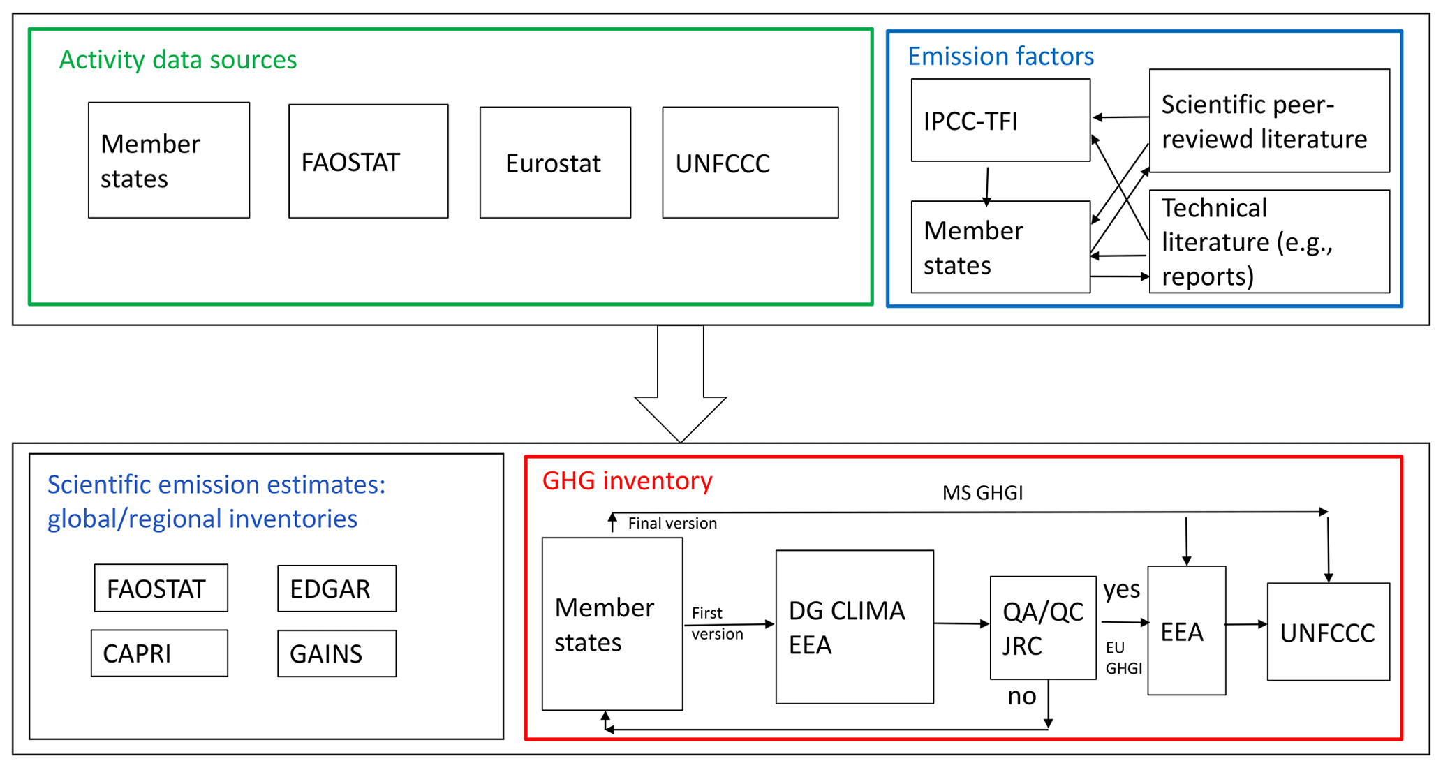
Figure 4 Example of flow of AD, EFs and emission estimates in the EU based on IPCC regulations.

We therefore conclude that all inventory-based data sources are consistent with each other for capturing recent CH₄ emission reductions or that they are not independent because they use similar methodology with different versions of the same AD (Fig. 4), which is mostly the case for the EU28 countries. The AD follows also a different course than the emissions data (see Fig. 4). The AD used is highly uncertain due to the collection process from surveys and different national reporting systems. FAOSTAT statistics use a relative value of 20 % uncertainty that is within the range for the confidence interval that IPCC (2006) suggests.

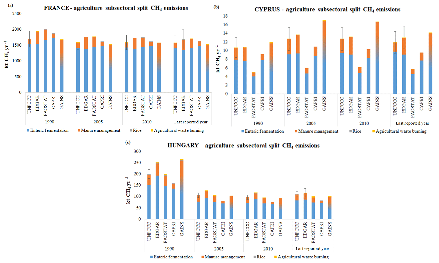
Figure 5 CH₄ emission from five data sources (UNFCCC NGHGI (2018), EDGAR v4.3.2, FAOSTAT, CAPRI and GAINS) split into main activities: enteric fermentation for ruminant livestock (blue) and manure management (orange). The GAINS gradient (orange–blue) represents the total emissions from enteric fermentation and manure management. Rice cultivation and agricultural field burning banned since 2000 are very small and hardly distinguishable in the plots; (a) very good consistency of the different data sources for France; (b) poor consistency for Cyprus; (c) high 1990 CH₄ emissions for Hungary (former eastern European block). The relative error on the UNFCCC values is computed with the method described in Appendix C based on the NGHGI 2018 uncertainties for the agriculture CH₄ data reported to UNFCCC. Uncertainty for EDGAR v4.3.2 was calculated for 2012 and represents the 95 % confidence interval of a lognormal distribution as described in Appendix B. The positive values represent a source. Last reported year in this study refers to 2016 (UNFCCC and FAOSTAT), 2012 (EDGAR), 2015 (GAINS) and 2013 (CAPRI).

From the detailed analysis of CH₄ emissions split into sectoral information (Fig. 5) (all country data and figures are provided in the excel spreadsheet “Figures5,8_AppendixD_CH₄_N₂O_per_country” downloadable at https://doi.org/10.5281/zenodo.3662371 (Petrescu et al., 2020) for the former eastern European communist centralized economy block (Latvia, Lithuania, Estonia (former USSR), the Czech Republic, Poland, Romania and Hungary, East Germany), we notice very high CH₄ emissions for 1990 which afterwards show a constant decreasing trend. This is best explained by the dissolution of the Soviet Union (1989–1991) and the consequent structural changes in their economy. The worst match between data sources in the EU28 is found for Malta, Cyprus and Croatia, but their emissions represent in the UNFCCC reporting less than 1 % of the total EU28 agricultural CH₄ emissions. UNFCCC uncertainties for CH₄ emissions are between 10 % and 50 % but can be larger for some countries and sectors, e.g., Romania reporting a 500 % uncertainty for emissions from rice cultivation.

To exemplify the shares of CH₄ emission from agriculture, in Fig. 5 we present the total subsectoral CH₄ emissions for three example countries.

The highest share is attributed to enteric fermentation, which for almost all countries counts as ∼ 80 % of total agricultural CH₄ emissions. We notice that a very good consistency between emission estimates is found in Fig. 5a for France, while on the contrary a worse consistency is presented in Fig. 5b for Cyprus, which might not report AD to FAOSTAT from its entire territory. Figure 5c exemplifies the high 1990 CH₄ emissions for Hungary in the former eastern European block and the lower subsequent estimates, mainly caused by political and economic changes after the dissolution of the Soviet Union (1989–1991). Note that some eastern European countries, i.e., Romania and Bulgaria, used different base years for Kyoto (1989 and 1988 respectively, footnote 3), as statistical data were considered problematic for 1990.

3.1.2 N₂O emissions

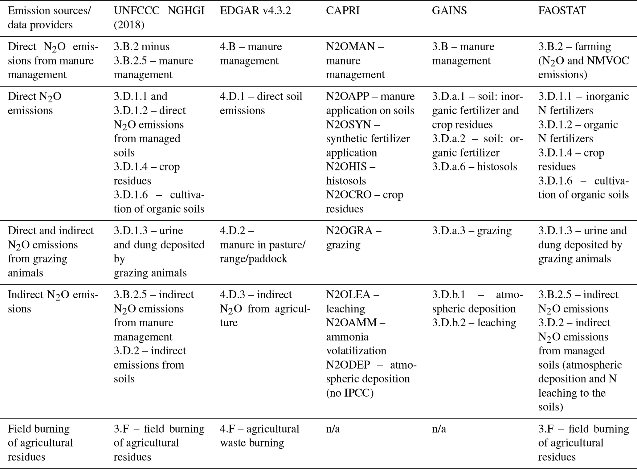
According to UNFCCC NGHGI (2018) data, in 2016 agricultural activities accounted for 78 % of the total N₂O emissions in the EU28. For the agriculture sector, key categories on the EU28 level are N₂O emissions from manure management, direct N₂O emissions from agricultural soils and indirect N₂O emissions from agricultural soils. In Table 3 we present the allocation of emissions by subsector following the IPCC classification, and we notice that each data source has its own particular way of grouping emissions.

Table 3 Agricultural N₂O emissions – allocation of emissions in different sectors by different data sources.

Similar to CH₄ emissions, N₂O emissions show very good consistency between the five data sources for total EU28 emissions (Fig. 6). We note as well that uncertainties of UNFCCC and EDGAR are large but have similar magnitudes. Similar to CH₄, CAPRI has the lowest estimate but well within the uncertainty interval.

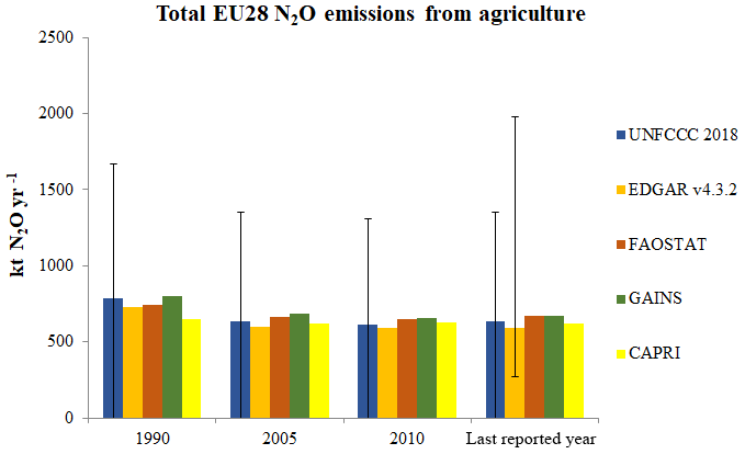
Figure 6 Total EU28 agriculture N₂O emissions from five data sources: UNFCCC NGHGI (2018), EDGAR v4.3.2, FAOSTAT, CAPRI and GAINS. The relative error on the UNFCCC value, computed with the 95 % confidence interval method, is 106 %. It represents the NGHGI 2018 uncertainty for the EU28 total N₂O agriculture data reported to UNFCCC. EDGAR uncertainty is only calculated for the last available year, 2012. Last reported year in this study refers to 2016 (UNFCCC and FAOSTAT), 2012 (EDGAR), 2015 (GAINS) and 2013 (CAPRI). The positive values represent a source.

In Fig. 7 we present the N₂O emission difference between 2005 and 1990, as well as between the last reported year, 2012 (the last common year in reporting for all data sources), 2010 and 2005. We observe that for the 2005–1990 change there is a major reduction in N₂O emissions for all data sources for the same reasons stated for CH₄, but the spread between different reduction estimates is much larger than for CH₄. We do not see the same agreement for the reduction between 2010, 2012 and 2005 (i.e., CAPRI shows a small increase and other datasets a net decrease) and between the last reported year and 2005 (i.e., FAOSTAT and CAPRI show small increases). The differences between the last reported year and 2005 could be partly attributed to the fact that the data sources have a different last reported year (see Table 1, in bold).

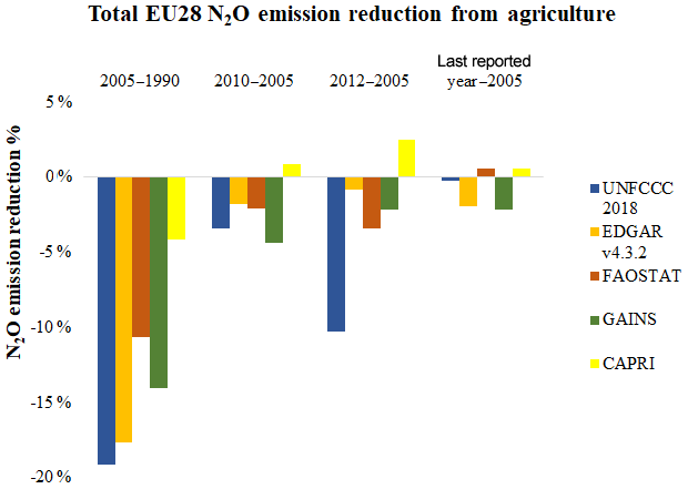
Figure 7 Change in EU28 total agricultural N₂O emissions between different years. The year 2012 is the last common year when all sources report estimates. Last reported year in this study refers to 2016 (UNFCCC and FAOSTAT), 2012 (EDGAR), 2015 (GAINS) and 2013 (CAPRI).

Nevertheless, despite the inconsistent sign of N₂O emission changes between datasets, the spread between absolute values of N₂O emission changes is smaller for recent periods than for the period 1990–2005. For both CAPRI and FAOSTAT, the increase in N₂O emissions, well represented by the positive changes seen in Fig. 7, can be explained by changes in AD from synthetic fertilizers and correlated increment of crop residues.

The two most important sources for N₂O emissions from agriculture pertain to direct (synthetic fertilizer, manure application to soils, histosols, crop residues and biological nitrogen fixation) and indirect (ammonia volatilization, leaching and atmospheric deposition) emissions. We exemplify this in Fig. 8, where we present the N₂O split in subactivities.

We notice for the eastern European former communist centralized economy block (all country data and figures are provided in the excel spreadsheet “Figures5,8_AppendixD_CH₄_N₂O_per_country.xlsx” downloadable at https://doi.org/10.5281/zenodo.3662371; Petrescu et al., 2020) – e.g., former USSR countries, i.e., Latvia, Lithuania and Estonia; and former eastern European block, i.e., Romania, Hungary, Slovakia and Bulgaria – higher N₂O emissions for 1990 which afterwards show a constant decreasing trend. This is again best explained by the economic transition in 1989–1991 and consequent impacts on the agriculture sector. The poorest consistency between data sources in the EU28 is seen for Belgium, Estonia, Lithuania, Latvia and Luxembourg (Figures5,8_AppendixD_CH₄_N₂O_per_country.xlsx), but their emissions count for as much as 4.5 % of total EU28 N₂O emissions. In general, the uncertainties reported to UNFCCC for total N₂O emissions from the agriculture sector are very high and have a range between 22 % (Malta) and 207 % (Romania). For subactivities, extreme uncertainties are reported by Denmark and Bulgaria as 300 % for N₂O emissions from manure management, while Greece reports a very small uncertainty of less than 2 % for N₂O emissions from agricultural soils.

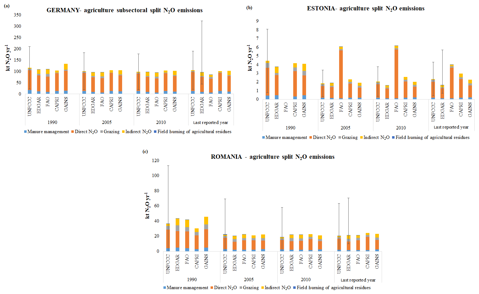
Figure 8 N₂O emission from agriculture split into main activities: manure management, direct emissions, grazing, indirect emissions and field burning of agricultural residues; (a) very good consistency for Germany; (b) poor consistency for Estonia; (c) high 1990 N₂O emissions for Romania (former eastern European block). The relative error on the UNFCCC values is computed with the method described in Appendix C based on the NGHGI 2018 uncertainties for the agriculture N₂O data reported to UNFCCC. Uncertainty for EDGAR v4.3.2 was calculated for 2012 and represents the 95 % confidence interval of a lognormal distribution as described in Appendix B. The positive values represent a source. Last reported year in this study refers to 2016 (UNFCCC and FAOSTAT), 2012 (EDGAR), 2015 (GAINS) and 2013 (CAPRI).

EDGAR is using data from FAOSTAT; thus, for the majority of countries (figures found as described in Appendix D), we observe similar estimates between these two sources (e.g., France, Italy, Poland). A reason for discrepancies may be attributed to the different way the data sources allocate their emissions to subactivities (Table 3). For example, CAPRI N2OSYN – synthetic fertilizer application – does not have a correspondent in GAINS activities. The leaching, ammonia and atmospheric deposition N₂O emissions in CAPRI do not have a clear correspondent subactivity in UNFCCC, while in FAOSTAT those N₂O emissions are reported under other categories: manure left on pasture and manure applied to soils.

For N₂O emissions, uncertainties are mostly in the range of 100 % or more. The countries reporting the highest N₂O uncertainties are Bulgaria, Denmark, Estonia and Cyprus, which, for manure management and agricultural soils, count as much as 200 % to 300 %. We notice that a very good match between emission estimates is found in Fig. 8a for Germany, while on the contrary a worse match is presented in Fig. 8b for Estonia, with no FAO data available in 1990 (only for former USSR). Figure 8c exemplifies the high 1990 N₂O emissions for Romania (former eastern European block), which is due to irregularities in reporting during the dissolution of the Soviet Union (1989–1991).

3.2 Natural CH₄ emissions

In recent assessments of the global CH₄ budget (Saunois et al., 2019), wetlands CH₄ emissions from top-down and bottom-up estimates for the period 2008–2017 are statistically consistent and average 178 Tg CH₄ yr⁻¹ (range 155–200) and 149 Tg CH₄ yr⁻¹ (range 102–182), respectively (Saunois et al., 2019).

In the EU28, natural emissions of CH₄ are represented by wetlands which are not yet fully accounted for and reported under NGHGIs, their emissions reporting being only recommended under the 2013 IPCC Wetlands Supplement (IPCC, 2014) complement to 2006 IPCC GL. According UNFCCC NGHGI (2019), between 2008 and 2017, the natural CH₄ emissions in the EU28 reported under LULUCF (CRF Table 4(II) accessible for each EU28 country⁶) summed up to 0.1 Tg CH₄. The only countries in the EU28 reporting CH₄ from wetlands were Denmark, Finland, Germany, Ireland, Latvia and Sweden.

Wetlands are sinks for CO₂ and sources of CH₄. Their net GHG emissions therefore depend on the relative sign and magnitude of the land–atmosphere exchange of these two major GHGs. Undisturbed wetlands are thought to have a large carbon sequestration potential because near-water-logged conditions reduce or inhibit microbial respiration, but CH₄ production may partially or completely counteract carbon uptake (Petrescu et al., 2015). The net GHG balance of natural wetlands is thus uncertain. Natural emissions of CH₄, in particular wetlands and inland waters and their net GHG balance, are the most important source of uncertainty in the methane budget (Saunois et al., 2019), due to the GWP100 of CH₄ and the generally opposite directions of CO₂ and CH₄ fluxes.

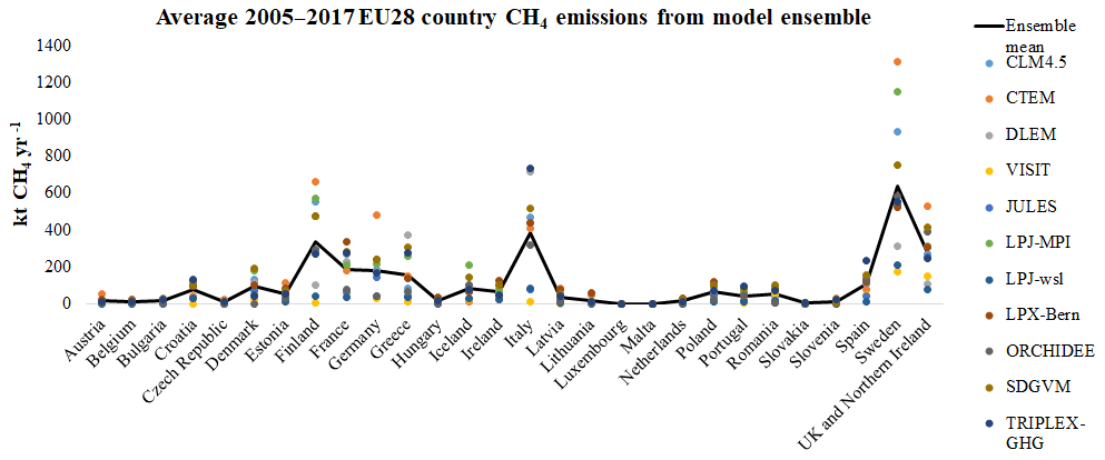
Figure 9 Distribution of CH₄ emissions from undisturbed natural wetlands for all the countries of EU28 as simulated by an ensemble of 11 global emission models averaged between 2005 and 2017 (Poulter et al., 2017). The positive values represent a source. The models are explained in the acronym list and referenced in Appendix B.

Under the new EU LULUCF Regulation article 7 (footnote 7), the accounting of natural wetland emissions will become mandatory from 2026 onwards; i.e., the reported numbers will be compared to numbers already reported under category 4(II) wetlands between 2005 and 2009, and the net difference will count towards reaching the EU climate targets.

Since CH₄ emissions are highly variable in time and space as a function of climate and disturbances, it makes EF-based methods impractical and national budget estimates difficult, making it challenging to accurately estimate CH₄ emissions in NGHGIs. There is also a risk of double counting with emissions from inland waters as discussed, e.g., by Saunois et al. (2019) for the global CH₄ budget. The sum of all natural sources of CH₄ as inferred by different models may be too large by about 30 % compared to the constraint provided by global inversions. The spread of wetland emissions from process-based wetland emission models used in the global CH₄ budget (Poulter et al., 2017) forced by the same variable flooded area dataset is 30 % (80 Tg CH₄ yr⁻¹) globally (given their estimated emissions of 177–284 Tg CH₄ yr⁻¹ using bottom-up modeling approaches), up to 70 % for the EU28 calculated based on the model-to-model variability and even larger at a national scale. In the absence of any better information, we used in this study the results of these ensemble models (see Appendix B) to provide a first estimate of this source.

According to Poulter et al. (2017), between 2005 and 2017, the total wetland CH₄ emissions in the EU28 averaged 3 Tg CH₄ with an uncertainty (1σ spread) of 70 %, with seven countries having the highest emissions (Fig. 9). Finland, Italy, Sweden, UK, France, Greece and Germany accounted for 75 % of total EU28 wetland CH₄ emissions. For the same period, UNFCCC NGHGI 2019 reports an average of 10.34 kt CH₄ (0.01 Tg CH₄), a highly underestimated value compared to the modeled results, due to nonreporting and accounting under NGHGIs.

Given this current gap between modeled and NGHGI reported data on CH₄ emission from wetlands in the EU28, we stress the need of investing in better modeling methodologies for emission calculation and verification. Out of all EU28 countries, for the purpose of reporting, only Finland developed its own biogeochemical CH₄ model to provide to NGHGIs a very detailed list of estimates for all CH₄ subactivities.

3.3 Forestry and other land uses

The forestry and other land uses, referred to here as the LULUCF section, include CO₂ emissions and removals from forests (including soils and harvested wood products) and soil organic carbon (SOC) changes from grasslands and croplands. A comprehensive assessment of the overall carbon stocks and fluxes of forests would need to be complemented by the analysis of climate change impacts on forest productivity and composition (Lindner et al., 2015). Several studies analyzed the European forest carbon budget from different perspectives and over several time periods using GHG budgets from fluxes, inventories and inversions (Luyssaert et al., 2012), flux towers (Valentini et al., 2000), forest inventories (Liski et al., 2000; Nabuurs et al., 2018; Pilli et al., 2017), and IPCC GLs (Federici et al., 2015).

Table 4 Model descriptions and their references therein.

Achieving the well-below-2 ^∘C temperature goal of the PA requires, among others, negative emission technologies, low-carbon energy technologies and forest-based mitigation approaches (Grassi et al., 2018a; Nabuurs et al., 2017). Currently, the EU28 forests act as a sink, and forest management will continue to be the main driver affecting the productivity of European forests for the next decades (Koehl et al., 2010). Forest management, however, can enhance (Schlamadinger and Marland, 1996) or weaken (Searchinger et al., 2018) this sink. Furthermore, forest management not only influences the sink strength, it also changes forest composition and structure, which affects the exchange of energy with the atmosphere (Naudts et al., 2016) and therefore the potential of mitigating climate change (Luyssaert et al., 2018; Grassi et al., 2019).

We compared net CO₂ emissions and removals from the LULUCF sector reported by UNFCCC NGHGI (2018) to those included in FAOSTAT and to the carbon balance here termed as the net biome production (NBP) from different models (Table 4). Categories presented in this study are forest land, cropland and grassland. We present separately the results from forest land and land use, because some models (e.g., CBM and EFISCEN) use a different definition of forest land than the DGVMs ensemble TRENDY (Sitch et al., 2008; Le Quéré et al., 2009) or bookkeeping models (Houghton and Nassikas, 2017; Hansis et al., 2015).

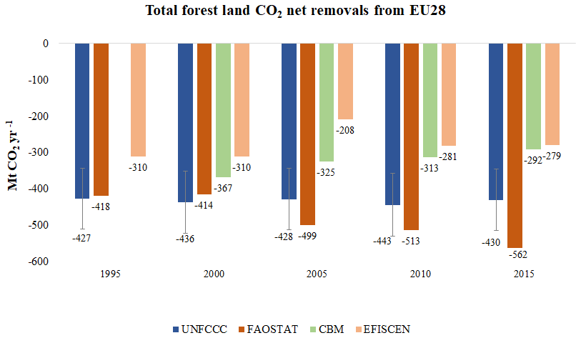
Figure 10 Total EU28 single-year values of CO₂ net removals from forest land (FL) as reported by UNFCCC, CBM, EFISCEN and FAOSTAT. Negative numbers denote net CO₂ uptake. EFISCEN data for 1995–2000 are based on Karjalainen et al. (2003) estimates. For 2005, 2010 and 2015, EFISCEN does not report numbers for Cyprus, Greece and Malta. EFISCEN reports only in 2015 numbers for CZE. For all years, CBM does not report numbers for Cyprus and Malta. CBM does not report data for 1995. The relative error on the UNFCCC value, computed with the 95 % confidence interval method, is 19.6 %. It represents the NGHGI 2018 uncertainty for the FL data pool reported to UNFCCC.

To better illustrate differences between estimates we exemplify how four of the data sources interpret and calculate the NBP:

• UNFCCC NBP definition depends on the method used by each country.

• CBM calculates NBP as the total ecosystem stock change calculated as the difference between net ecosystem production (NEP) and the direct losses due to harvest and natural disturbances (e.g., fires) (Pilli et al., 2017; Kurz et al., 2009). Adding to the NBP the total changes in the harvested wood product (HWP) carbon stock, CBM estimates the net sector exchange (NSE) (Karjalainen et al., 2003; Pilli et al., 2017).

• EFISCEN's NBP is derived from total tree gross growth minus (density related) mortality minus harvest, minus turnover of leaves, branches and roots. From input of litter minus decomposition, the soil balance is calculated with the Yasso soil model (Liski et al., 2005). Natural disturbances tend to occur relatively rarely in Europe and, when happening, are included in regular harvest; therefore EFISCEN does not consider them in addition for the NBP calculation.

• DGVMs calculate NBP as the net flux between land and atmosphere defined as photosynthesis minus the sum of plant and soil heterotrophic respiration, carbon fluxes from fires, harvest, grazing, land use change and any other C flux in/out of the ecosystem (e.g., dissolved inorganic carbon, DIC; dissolved organic carbon, DOC; and volatile organic compounds, VOCs). Land use change emissions are calculated as the imbalance between photosynthesis and respiration over land areas that followed a transition. NBP should be equal to changes in total carbon reservoirs. The net land use change flux is derived by differencing the NBP of a simulation with and without land use change.

3.3.1 Forest land

Net CO₂ emissions/removals from forest land (FL) (in UNFCCC NGHGI, 2018, IPCC sector 4.A) include net CO₂ emissions/removals from forest land remaining forest land and conversions to forests; i.e., it includes effects from both environmental changes and from land management and land use change as long as they occur on forest land declared as managed. According to 2006 IPCC GLs, to become accountable in the UNFCCC NGHGI under forest land remaining forest land, a land must be a forest for at least 20 years. Over FL we compare modeled NBP estimates (presented as CO₂ net sink) simulated with CBM and EFISCEN models with UNFCCC and FAOSTAT data consisting of net carbon stock change in the living biomass pool (aboveground and belowground biomass) associated with forest and net forest conversion including deforestation.

Figure 10 presents the total net CO₂ sink estimates simulated with CBM and EFISCEN models (described in Table 4 and Appendix B), FAOSTAT, and countries' official reporting done under UNFCCC. The sign convention is that negative numbers are a sink. The results show that the differences between models are systematic, with EFISCEN and CBM showing systematically lower sinks than UNFCCC, while FAOSTAT has systematically higher sinks and the FAOSTAT sink is increasing with time. The similarities between EFISCEN and CBM models are that they use National Forest Inventory (NFI) data as the main source of input to describe the current structure and composition of European forests. However, CBM and EFISCEN models make different assumptions about allometry, wood density or carbon content of trees. The difference between all estimates and FAOSTAT is probably because the stock change calculations directly use as input the carbon stocks and area data computed by countries and submitted through the FAO Global Forest Resource Assessments (FRA⁷), rather than employing models to estimate them. Further, FAOSTAT numbers include afforestation, i.e., the sum of all other land converted to FL, while the others datasets do not, resulting in a smaller sink if afforestation is removed.

Figure 11 Total EU28 net CO₂ emissions/removals from FAOSTAT and UNFCCC NGHGI (2018) submission estimates of cropland and grassland for 1990, 2015, 2010 and 2016. The relative error on the UNFCCC value, computed with the 95 % confidence interval method, is 53 %. It represents the NGHGI 2018 uncertainty for the CL and GL data pool reported to UNFCCC.

The UNFCCC NGHGI (2018) uncertainty of CO₂ estimates for FL at the EU28 level, computed with the 95 % confidence interval method (IPCC, 2006), is 19.6 %, with uncertainty increasing to 25 %–50 % when analyzed at the country level (EU NIR, 2014). Given that both CBM and EFISCEN use different methodologies to estimate emissions and removals (Pilli et al., 2016; Petz et al., 2016), likely leading to lower estimates than the NGHGI, we consider the match between the two models and the UNFCCC NGHGI 2019 estimates to be satisfactory, given the uncertainties and similarity in temporal trends.

From Fig. 10 we see that while UNFCCC estimates are very stable, FAOSTAT shows an increasing sink, while CBM and EFISCEN show a saturating sink. And although all four are based on almost the same raw data, estimates differ by up to 50 %. The sink of EFISCEN is somewhat lower because a higher harvesting was implemented in these runs. In 2015, most of the differences between FAOSTAT estimates and UNFCCC country data were generated by a few countries. For Finland, FAOSTAT reports around zero sink and UNFCCC reports a large sink of 38 Mt CO₂ yr⁻¹. For Romania and Latvia, the FAOSTAT sink is 165 and 17 Mt CO₂ yr⁻¹ respectively, a factor of 7 larger than the reported UNFCCC, 22 and 2.4 Mt CO₂ yr⁻¹ respectively. For Denmark, we find a sink according to FAOSTAT (−2.2 Mt CO₂) and a very small source reported to UNFCCC (0.17 Mt CO₂). When comparing NGHGI and FAOSTAT data, it should be considered that NGHGIs specifically report to the UNFCCC emissions and removals on managed forest land and are as such formally reviewed annually. By contrast, FAOSTAT emissions estimates include carbon stock changes over the total forest land area and are not part of the UNFCCC formal reporting and review process (Grassi et al., 2017).

3.4 Cropland and grassland soil carbon

Cropland and grassland (CL and GL) (in UNFCCC NGHGI, 2018, IPCC sector 4B and 4C, respectively) include net CO₂ emissions/removals from soil organic carbon (SOC) under the remaining and conversion categories. Similar to FL, fluxes include effects from both environmental changes and from land management and land use change. FAOSTAT GHG emissions in the domain cropland and grassland are currently limited to the CO₂ emissions from cropland/grassland organic soils associated with carbon losses from drained histosols under cropland/grassland. This can be one of the reasons for differences between estimates reported by the two sources (Fig. 11).

The cropland definition in IPCC includes cropping systems, and agroforestry systems where vegetation falls below the threshold used for the forest land category, consistent with the selection of national definitions (IPCC glossary). According to EUROSTAT, the term “crop” within cropland covers a very broad range of cultivated plants. In 2015 more than one-fifth (22 %) of the EU28's area was covered by cropland (EUROSTAT, available at https://ec.europa.eu/eurostat/statistics-explained/index.php/Land_cover_statistics, last access: January 2020). Denmark (51 %) and Hungary (44 %) had the highest proportion of their area covered by cropland in 2015. For the vast majority of the EU member states (MS), cropland accounted for between 15 % and 35 % of the total area, with this share falling to 10 %–15 % in Latvia, Estonia and Portugal, while the lowest proportions were registered in Slovenia (9 %), Finland (6 %), Ireland (6 %) and Sweden (4 %). In absolute terms, France, Germany, Spain and Poland had the biggest areas of cropland in 2015.

Grassland definition in IPCC includes rangelands and pasture land that is not considered cropland, as well as systems with vegetation that fall below the threshold used in the forest land category. This category also includes all grassland from wild lands to recreational areas as well as agricultural and silvopastoral systems, subdivided into managed and unmanaged, consistent with national definitions. Grasslands tend to be concentrated in regions with less favorable conditions for growing crops or where forests have been cut down. Some of these are found in northern Europe (e.g., Finland and Sweden), while others are in the far south, i.e., the south of Spain.

In 2015 just above one-fifth of the EU28's area (21 %) was covered by grassland. There is a broad range across EU member states, with Ireland having 56 % of its total land area as grassland and Finland and Sweden less than 6 % of the land (EUROSTAT, https://ec.europa.eu/eurostat/statistics-explained/index.php/Land_cover_statistics, last access: January 2020).

Figure 11 shows that in the EU28 croplands and grasslands are CO₂ sources to the atmosphere in the UNFCCC NGHGI (2018) and FAOSTAT databases. Cropland CO₂ emissions are rather stable with time and are in good agreement between FAOSTAT and UNFCCC, except in 1990. Grassland emissions reported by countries to UNFCCC are higher than the FAOSTAT and show an abrupt increase in 2016 compared to the previous years. The high estimates of grassland emissions in 2016 UNFCCC NGHGI submissions are explained by increased emissions in Austria, Denmark and Croatia; Sweden changed from being a sink in 2015 to being a very high source in 2016, and Hungary and Greece reported a lower sink. Ireland was the only country which reported a higher sink in 2016 compared to 2015.

Climate change and climate effects on soil temperature and moisture are key drivers in the 21st century increase in soil decomposition and decrease in the soil carbon stock (Smith et al., 2005). Avoiding soil carbon losses or restoring stocks requires practices that increase C input in excess of losses from erosion and decomposition, such as diminished grazing intensity for grasslands, higher return of residues or reduced tillage for croplands, and manure additions for both. Further change in land use and management will also affect the soil carbon stock of European cropland and grasslands (Smith et al., 2005).

3.5 Land-related emissions from global models

Land-related carbon emissions can also be estimated by global models such as DGVMs (here we used the TRENDY v6 ensemble) and two bookkeeping models (BLUE and H&N). In this section we compare these global model results with data from FAOSTAT and UNFCCC NGHGI (2018). There is significant uncertainty in the underlying datasets of land use changes, the coverage of different land use change practices and the calculation of carbon fluxes. In addition, marked differences in definitions must also be considered to compare independent estimates. Bookkeeping models give net emissions from land use change, including immediate emissions during land conversion, legacy emissions from slash and soil carbon after land use change, regrowth of secondary forest after abandonment, and emissions from harvested wood products when they decay. DGVMs estimate net land use emission as the difference between a run with and a run without land use change, and their estimate includes the loss of additional sink capacity, that is, the sink that favors the environmental changes (e.g., CO₂ fertilization). This sink created over forest land in the simulation without land use change is “lost” in the simulation with land use change because agricultural land lacks the woody material and thus has a higher carbon turnover (Gasser et al., 2013; Pongratz et al., 2014). This different definition from bookkeeping models historically implies higher carbon emissions from DGVMs, even if all postconversion carbon stock changes were the same in DGVMs and bookkeeping models.

The key difference between DGVMs and bookkeeping models, on the one hand, and FAO and UNFCCC methodologies, on the other, is that the latter are based on the managed land proxy (Grassi et al., 2018a) (Fig. 12).

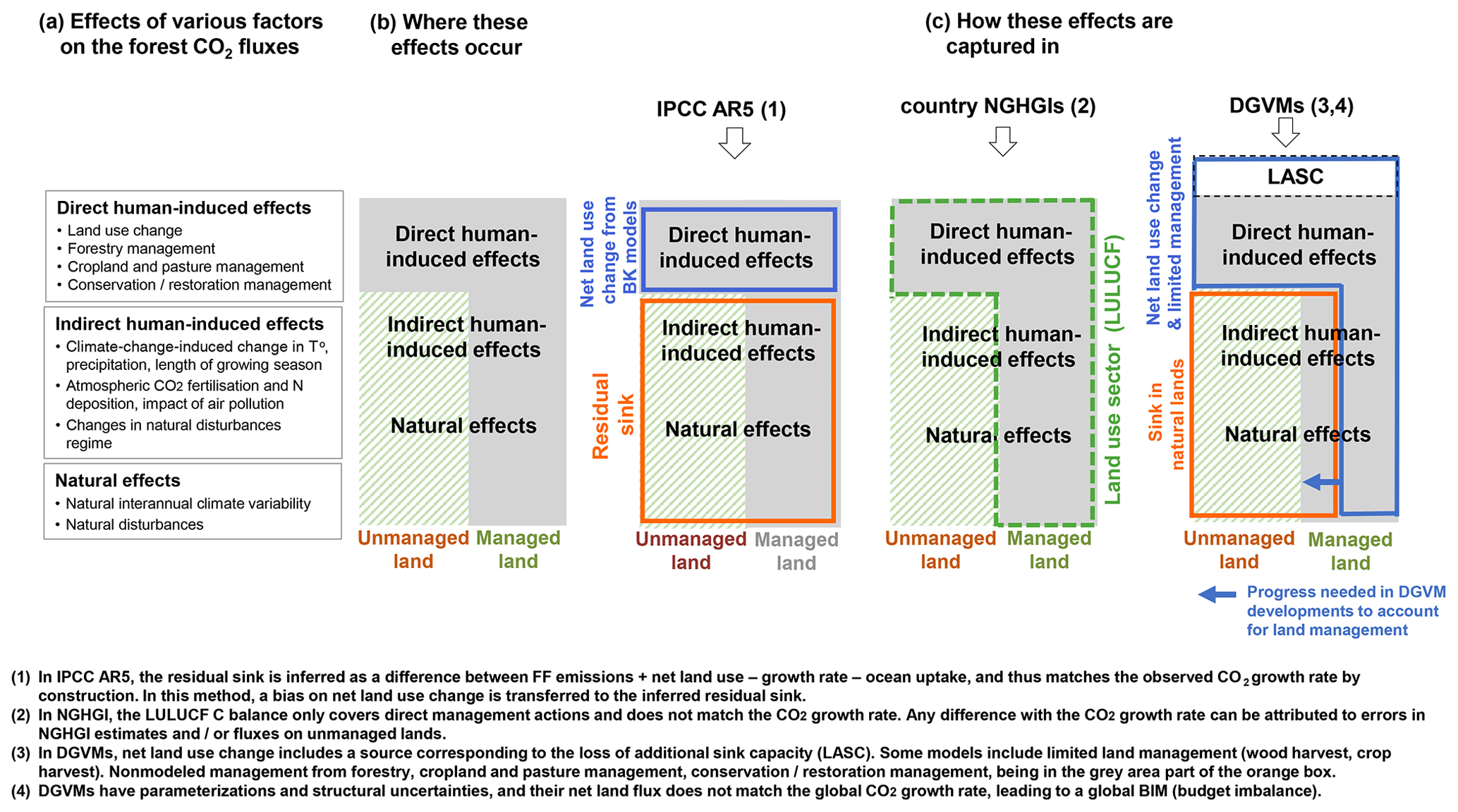
Figure 12 Summary of the main conceptual differences in defining the anthropogenic land CO₂ flux between the IPCC Fifth Assessment Report (AR5) and countries' GHG inventories (NGHGIs). (a) Effects of key processes on the land flux as defined by IPCC. (b) Where these effects occur (in unmanaged/primary lands vs. managed/secondary lands). (c) How these effects are captured: in the IPCC AR5 the anthropogenic net land use from Grassi et al. (2018a) (solid blue line, including only direct human-induced effects), and the nonanthropogenic residual sink (solid red line, calculated by the difference from the other terms in the GCB); countries' anthropogenic land flux from NGHGIs reported to UNFCCC (under the LULUCF sector, green dashed line), which in most cases includes direct and indirect human-induced and natural effects in an area of managed land that is broader than the one considered by Grassi et al. (2018a). (Figure adapted from Fig. 3 in Grassi et al., 2018a); DGVMs modeled anthropogenic land flux (solid blue line, including only direct human-induced effects and partly as managed land) and the nonanthropogenic residual sink (solid red line) partly covering the managed land. DGVMs simulate the net CO₂ flux from land use change by the difference between a simulation with variable land cover and a simulation with fixed land cover at the beginning of the simulation period. In the latter, ecosystems that are not converted are a foregone sink of CO₂, causing the so-called loss of additional sink capacity (LASC).

Land fluxes can be differentiated into three processes (IPCC, 2010): (1) direct anthropogenic effects (land use and land use change, e.g., harvest, other management, deforestation), (2) indirect anthropogenic effects (e.g., changes induced by human-induced climate change, including CO₂ fertilization and nitrogen deposition changes), and (3) natural effects (i.e., that would happen without human-caused climate change, such as natural disturbances).

Models and GHGIs capture these effects in a different way:

• Biogeochemical models. Bookkeeping approaches only estimate direct anthropogenic effects. DGVMs also consider fluxes linked to indirect effects and natural processes. In the GCB 2018 (Le Quéré et al., 2018b) and GCB 2019 (Friedlingstein et al., 2019), the fluxes associated with the direct anthropogenic effects are estimated with bookkeeping models and DGVMs, while the remaining land sinks (including all indirect and natural effects) are estimated by DGVMs.

• National Greenhouse Gas Inventories (UNFCCC NGHGIs). These inventories use the notion of managed land as a proxy for anthropogenic emissions (IPCC, 2006) and hence in practice include most or all (depending on the specific method) indirect emissions into their anthropogenic estimates. In addition, the area considered managed by countries is typically much greater than the area used by biophysical models to simulate the direct anthropogenic effects, as it includes areas that are not actively managed (for instance, forest parks or forests seldom harvested) (Grassi et al.. 2018a).

The difference between biogeochemical models and NGHGIs of around 4–5 Gt CO₂ yr⁻¹ globally is to a large part attributable to the accounting of indirect effects on greater-area managed land by NGHGIs compared to models (Grassi et al., 2018a; IPCC, 2019b). The differences at the EU28 level are smaller, because most forest land is considered managed by both models and NGHGIs.

Independent estimates of the land-related flux for the EU28 are presented in Fig. 13. The data behind the three main estimates, bookkeeping models, NGHGIs and FAOSTAT represent the total net land use emissions/removal from forests, including conversions to and from one category to another. Next to them, we plotted each of the net land use change fluxes (in grey; difference of simulation with and without land use change) from eight of the TRENDYv6 DGVMs used in the GCB 2017 (Le Quéré et al., 2018a) with their mean, as they mostly simulate the indirect and natural sink considered unmanaged. FAOSTAT includes emissions from peatland drainage and fires and from biomass fires (not considered herein). It does not include however other carbon stock changes in cropland and grassland. We additionally excluded from the UNFCCC estimate the categories wetlands remaining wetlands and settlements remaining settlements, as well as biomass burning and drainage and transitions between nonforest lands.

The UNFCCC NGHGI (2018) and H&N's estimates are similar because the managed areas for the EU28 are similar in both estimates (Grassi et al., 2018a). Differences between the two bookkeeping models, BLUE and H&N, relate to the different input data applied by each of the models and differences in biome types. The input used by H&N is based directly on FAOSTAT agricultural and wood harvest data and FRA forest area changes, while BLUE uses LUH2 (Hurtt et al., 2011, 2020). LUH2 is based on HYDE3.2 (Klein Goldewijk et al., 2017a, b), which provides annual, 0.5^∘, fractional data on cropland and pasture based on FAOSTAT but overlays subgrid-scale transitions between all land use types and wood harvesting. H&N allocates pasture expansion preferentially on natural grasslands, while all available vegetation types of a grid cell are assigned proportionally to agricultural expansion in BLUE. Carbon densities and regrowth and decay curves are structurally similar but differ in detail.

The EU28 has a very small area of unmanaged land and this denotes that most of the LULUCF emissions in the EU28 are from direct effects in the forestry sector (including agricultural expansion/abandonment). According to FAOSTAT and UNFCCC NGHGIs, the net forest conversion is relatively small in the EU, so the simulations include mostly managed net area.

Figure 13 A comparison of different estimates of the land use change flux in the EU28 from five available data sources: BLUE, H&N, UNFCCC NGHGI (2018), DGVMs (TRENDY v6) and FAOSTAT. The grey lines represent the individual model data for eight DGVMs. The UNFCCC estimate includes the following categories: forest land, cropland, grassland net and with conversions and wetlands, settlements, and other land-only conversions. The FAOSTAT estimate includes the following categories: forest land remaining forest land, afforestation and deforestation (conversion of forest land to other land types). The negative values represent a sink, while the positive values represent a source.

DGVMs differ strongly in their estimate of the net land use change flux due to different comprehensiveness of including land use practices such as wood harvesting, shifting cultivation, or fire management (Le Quéré et al., 2018a); different land use change datasets (HYDE3.2 or LUH2) and their implementation; and general model differences of how photosynthesis, respiration, and natural disturbances are simulated. Most striking in comparison to the other, more empirical, approaches is the large interannual variability, related to the climate dependency of vegetation processes. Though DGVMs are conceptually similar to NGHGIs in simulating all indirect and direct fluxes on a given area, differencing of the simulations with and without land use change leaves only the land-use-related effects to be attributed to the net land use change flux (see Fig. 12). DGVMs are thus closer to the bookkeeping definition of LULUCF emissions, apart from differing assumptions on environmental changes (constant in bookkeeping, historical in TRENDY) and the loss of additional sink capacity included in DGVMs.

4 Discussion

4.1 Agricultural emissions

At the European level the largest inconsistencies between estimates from AFOLU emission sources/sinks were found to be mainly caused by the use of different methodologies, including use of different AD and/or tier level. When looking at final emission estimates, inconsistencies in methodology and tier application in calculating emissions give as much as 10 %–20 % variation across estimates (e.g., CH₄ from agriculture). Higher tiers require more detailed AD for calculating emissions/removals from AFOLU sectors.

Within the UNFCCC practice, for agriculture, each country uses its own country-specific method which considers specific national circumstances (as long as they are in accordance with the 2006 IPCC GLs) as well as IPCC default values, which are usually more conservative. The EU GHG inventory underlies the assumption that the individual use of national country-specific methods leads to more accurate GHG estimates than the implementation of a single EU-wide approach (UNFCCC, 2018). The tier level a country applies depends on the national circumstances, which explains the variability of uncertainties among the sector itself as well as among EU countries. For example, inventory estimates of N₂O emissions have very large uncertainties (> 100 %) owing to the heterogeneity of sources and uncertainty in emission factors for the main N₂O sources, in particular agriculture. Since agricultural soil and manure management emissions vary strongly from site to site depending on, e.g., soil properties and background emissions, management, and meteorology, it is extremely challenging to determine accurate mean emission factors (JRC report, https://ec.europa.eu/jrc/en/publication/eur-scientific-and-technical-research-reports/atmospheric-monitoring-and-inverse-modelling-verification-greenhouse-gas-inventories, last access: February 2020). Winiwarter et al. (2018) stated that, under current technologies, agricultural emissions have a large potential for abatement, and, in the short term, reductions of N₂O emissions must rely on the adoption of existing technologies. Currently available technology could reduce global N₂O emissions by about 26 % below the baseline projection in 2030 (Winiwarter et al., 2018). The most applicable pathways to enhance emission reductions are the refinements of existing options (use of fertilizers), increasing the efficiency of measures (N use efficiency) and changing human diets (lower consumption of animal protein). Oenema et al. (2013) estimated a total reduction potential for N₂O emissions from agriculture including human diet changes of up to 60 % in 2050, adding about half to the reductions available from technical measures alone (41 % reductions). For CH₄, according to Höglund-Isaksson et al. (2012) and the scenario work based on the GAINS model, mitigation opportunities in agriculture are found limited and often costly both from social and private cost perspectives.

Concerning the IPCC calculation of CH₄ emissions from enteric fermentation, depending on the type of animal, the situation within the EU28 varies from country to country. For cattle (IPCC sector 3.A.1) emissions are calculated with very sophisticated methods, with only Cyprus using partially Tier 1. For the enteric fermentation of sheep (3.A.2), the situation is more diverse, with 13 countries using Tier 1 methods and 15 using higher tiers (including those with higher emissions). For other cattle (3.A.4), only three countries (Romania, France and Portugal) are using higher tiers, with all the others combining different methods. CH₄ and N₂O emissions from manure management (3.B.1 and 3.B.2) are even more mixed, with Germany, Denmark, Finland, France, Croatia and Romania using exclusively higher tiers in both categories. For the calculation of emissions from soils, the share of high tiers is very low; only Denmark and Sweden use solely higher tiers in indirect N₂O emissions from agricultural soils (3.D.2), while there are no countries using only high tiers in direct N₂O emissions (3.D.1) but only some combining high with low tier methods (UNFCCC, 2018b). All these differences in calculating emissions produce evidently higher uncertainties in the results. For the UNFCCC, throughout the variability of the analyzed NGHGIs, it turned out that N₂O emissions from manure management and direct and indirect emissions together with CH₄ emissions from rice cultivation have the largest uncertainties. When we aggregated UNFCCC uncertainties at the country level (using the methodology described in Appendix C), we also noticed the fact that not all countries report subsectoral uncertainties (e.g., Greece for grazing) and some countries (Sweden, Poland, Croatia and the Czech Republic) had no uncertainty analysis performed for all subactivities due to lack of data (e.g., confidential data).

There is as well the need to define a common methodology for overall uncertainty calculation while checking for consistency in the way uncertainties are calculated for different data sources and the way data are aggregated for different sectors. We noticed that for agricultural N₂O emissions the split in subactivities is not always consistent with IPCC sectors, and this leaves room for differences when aggregating the results (Table 3).

4.2 Forestry and other land uses

For the LULUCF sector, methods for the estimation of GHGs and CO₂ fluxes still differ among countries and land use categories. Within the UNFCCC practice, strict good practice guidance is prescribed, but there are still small differences between countries as each considers specific national circumstances (as long as they are in accordance with the 2006 IPCC GLs), as well as IPCC default values. When we analyze the estimates from multiple sources (inventories and models) we observe that published estimates contain two main sources of uncertainties: (a) differences due to input data and structural/parametric uncertainty of models (Houghton et al., 2012) and (b) differences in definition (Pongratz et al., 2014; Grassi et al., 2018b). These differences result from choices in the simulation setup and are partly predetermined (for b) in particular) by the type of model used – bookkeeping models, DGVMs, or inventory based – and whether fluxes are attributed to LULUCF emissions due to the cause or place of occurrence (indirect fluxes on managed land included in NGHGIs and FAOSTAT). Differences in definitions and methodology calculation of estimates across model types are crucial and may lead to model-to-model variability. Depending on the degree of independence between assumptions, variability can become a reliable proxy for structural uncertainty when more accurate estimates are lacking (Solazzo et al., 2018). In Fig. 13 the variability between the mean of the DGVMs ranges between 44 % in 1996 and 186 % in 2016 (distance between interquartile range and median across models for each year).

In general the definition of NBP denotes the net gain or loss of carbon from a region. NBP is equal to the net ecosystem production (NEP) minus the carbon lost due to a disturbance (e.g., forest fire, harvest) taking into account as well the net C balance of harvested products (described by the 2006 IPCC GLs) and C emitted by inland waters. In the context of land use change, the GCB 2017 (Le Quéré et al., 2018a) highlighted harvest as one of the main uncertainties. As an example, according Nabuurs et al. (2018) the uncertainty affecting all studies is that EU harvesting levels are rather uncertain. According to the FRA report 2015 (FRA, 2015), most European countries have a solid forest inventory, but there is still large uncertainty over harvesting levels. For many countries forest statistics from FAO have shortcomings such as very large differences between reported periods, data corrected in later versions and unreported (harvest) removals (Nabuurs et al., 2018).

Checking collective progress towards meeting the goals of the PA will be done by the PA's global stocktake. At present, there is a discrepancy of about 4–5 Gt CO₂ yr⁻¹ in global anthropogenic net land use emissions (Grassi et al., 2018a; IPCCC, 2019b) between DGVMs reflected in IPCC assessment reports and aggregated national UNFCCC GHG inventories. Grassi et al. (2018a) shows that about 3.2 Gt CO₂ yr⁻¹ can be explained by conceptual differences in anthropogenic forest sink estimation, related to the representation of environmental change impacts and the areas considered managed. In order to limit the temperature increase to 1.5 ^∘C and keep it well below 2 ^∘C, as set by the PA, net-zero CO₂ emissions at the global level need to be achieved around 2050 and neutrality for all other GHGs somewhat later in the century. At this point, any remaining GHG emissions in certain sectors need to be compensated for by absorption in other sectors, with a specific role for the land use sector, agriculture and forests (European Commission Report, 2018).

It is important to distinguish between reporting and accounting in the GHG inventory context, as not all reported emissions account towards emission reduction efforts (Grassi et al., 2018b). Reporting refers to the inclusion of estimates of anthropogenic GHG fluxes in NIRs, following the methodological guidance provided by the IPCC. The NIR should, in principle, aim to reflect “what the atmosphere sees” (Peters et al., 2009) in managed lands, within the limits given by the method used and the data available. In the context of mitigation targets (e.g., the PA), accounting refers to the comparison of emissions and removals with the target and quantifies progress toward the target. For the LULUCF sector, specific accounting rules are used to filter reported flux estimates with the aim to better quantify the results of mitigation actions (Grassi et al., 2018b). The UNFCCC reporting principles allocate emissions to the territorial location (national boundaries) at the time that they occur (Peters et al., 2009).

The different definitions and concepts used by the global models and inventory communities mean that the land fluxes cannot necessarily be consistently compared. The framework developed by Grassi et al. (2018a) and shown in Fig. 12 can be generalized to make a more direct comparison as applied to EU28 (Fig. 14). Figure 14 disaggregates managed forest land into components that are reported in the UNFCCC CRFs: converted land (e.g., land changing from cropland to forest land) and the remaining land (e.g., forest land remaining forest land) are split into land that is “production” (remaining forestry, RF) or land that is used for ecological or social functions (other R_o), based on the definitions of managed land. Unmanaged land (sink, S) cannot have direct human-induced effects.

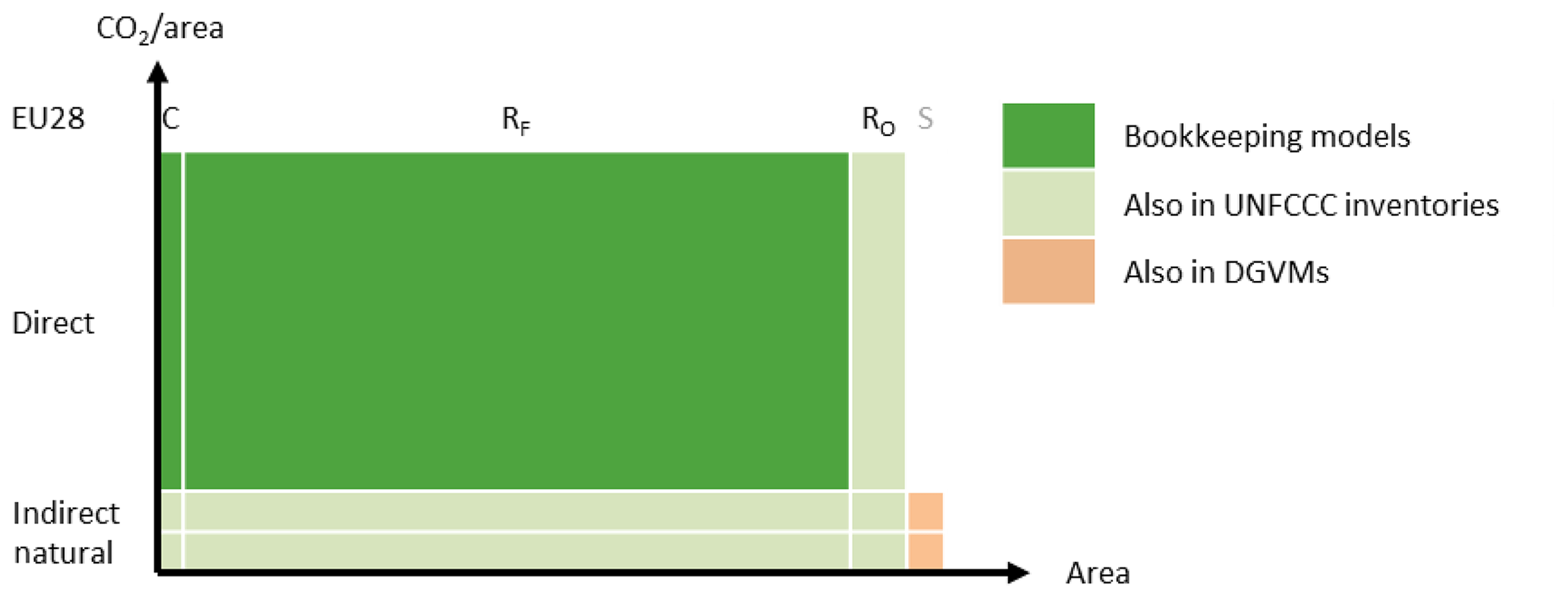
Figure 14 A conceptual extension of Fig. 12, applied to EU28, to disaggregate the managed land into the components reported in the UNFCCC inventories. The vertical axis represents density, the horizontal axis represents the area and the area of each box is the CO₂ emissions. The diagram is conceptual and not to scale, but it does give an indication of how the components may look in the EU28. The converted land (C) is equivalent to afforestation plus deforestation. Remaining land is split into remaining forestry (RF) and remaining other (ecological and social functions) (R_o), and the sink (S) belongs to unmanaged land. Bookkeeping models consider only direct effects (dark green) but do not include transitions between cropland and pasture or land management changes (increasing tillage, introducing irrigation, etc.). UNFCCC CRFs include all dark- and light-green components (direct, indirect, natural on managed land), while DGVMs in principle can include all components including the sink (pink).

Overall, our results suggest that most of the LULUCF emissions in the EU28 are from direct effects in the managed forest sector, including age-legacy effects (forest expansion and regrowth after WWII), with small net emissions from land conversion as they are largely compensated for by deforestation (from CRFs). With appropriate data and models, it is theoretically possible to expand and enumerate the estimates more accurately.

5 Data availability

All raw data files reported in this work which were used for calculations and figures are available for public download at https://doi.org/10.5281/zenodo.3662371 (Petrescu et al., 2020). The data we submitted are reachable with one click (without the need for entering login and password), with a second click to download the data, consistent with the two-click access principle for data published in ESSD (Carlson and Oda, 2018). The data and the DOI number are subject to future updates and only refers to this version of the paper.

6 Conclusions

There are many independent estimates of GHG emissions, but adequate understanding of their differences (either qualitatively or quantitatively) is lacking. For CH₄ and N₂O emissions the main differences between country reports and models are the use of tiers and methodologies (for both emissions and uncertainty calculation). Countries reporting to UNFCCC use an inconsistent mix of tiers depending on the animal type and activity following the approach described by the 2006 IPCC GLs, while models run with more accurate data and have better disaggregation of activities. One detected similarity between all sources is the use of EFs, as almost all sources make use of the IPCC defaults. AD are often shared, mostly sourced from the MS, FAOSTAT, Eurostat or UNFCCC, with the reasons for differences in activity data between these four sources not totally understood.

At the EU28 level, there is room to improve NGHGIs' consistency between UNFCCC tier use and models (e.g., 10 %–20 % difference for CH₄ from agriculture). We stress the need for more detailed quantification of the difference between LULUCF CO₂ estimates (inventories, models, etc.) caused by inconsistencies in methodology and/or tier application. More data and analysis are needed to account for and reduce the differences in estimates. Narrowing down the analysis to sensitive parameters (e.g., AD) which may trigger the differences (e.g., Appendix A, Table A1a,b) also requires more information on uncertainties.

It is of great importance to better distinguish between direct and indirect effects on land use emissions especially for the purpose of reconciling land-related emissions from global datasets and NGHGIs. Currently our comparisons give significant uncertainty, mostly related to coverage of different land use practices and the differences in definitions (Fig. 12).

It is important to recognize that just because independent inventories agree well for a sector does not necessarily mean that the estimate is closer to the actual emissions. The reason for agreement across inventories may simply be that the different inventories used the same methodology and data sources. In recent years there has been increased attention to the quantitative differences between land-based CO₂ emissions, with a much better understanding between inventories and estimates from the scientific community. However, there remain gaps in our understanding of differences between FAOSTAT and UNFCCC and between different DGVMs and bookkeeping models. One explanation can be linked to the fact that models use different methods to estimate emissions/removal than countries use in reporting to UNFCCC.

The current atmospheric GHG network is coordinated by the Integrated Carbon Observation System (ICOS) infrastructure at the European level. Within the future UNFCCC reporting framework, we argue that countries should use, whenever possible, global inversions to provide additional constraints for the verification and reconciliation purposes. A synthesis of available top-down non-CO₂ estimates has already been undertaken by Bergamaschi et al. (2015) and was not discussed here, but within the VERIFY project framework, we will use it in a following study focused on inversions based on better, higher-resolution, transport models to assimilate the precise ICOS GHG concentration data complemented by satellite retrievals of column CO₂, CH₄ and N₂O concentrations. While the GCP (Friedlingstein et al., 2019) provides the global carbon budget, this study starts a series of datasets for the EU. These are essential for the GHG monitoring and verification support capacity the EU envisages to build in support of the enhanced transparency framework of the Paris Agreement. The European Commission decided to take up a new service for monitoring anthropogenic CO₂ emissions under the long-term Copernicus Programme, which is under construction (Janssens-Maenhout et al., 2020) and will make use of regional inversions coupled with global inversions.

The main challenge for the inversion community remains the separation of the natural and anthropogenic part of the total emission column. For the moment, global inverse models are widely used to estimate emissions of CH₄ and N₂O at a global/continental scale, using mainly high-accuracy surface measurements at remote stations (e.g., Bergamaschi et al., 2013, 2018; Bousquet et al., 2006; Mikaloff Fletcher et al., 2004a, b; Saunois et al., 2016; Hirsch et al., 2006; Huang et al., 2008; Saikawa et al., 2014; Thompson et al., 2014; Wells et al., 2018) with few regional inversions used to mainly estimate the European CH₄ and N₂O emissions (Bergamaschi et al., 2015, 2018).

Appendix A: Methodology tables

Table A1 (a) Agriculture source-specific activity data (AD), emission factors (EF) and uncertainty methodology; (b) LULUCF source-specific activity data (AD), emission factors (EF) and uncertainty information. “n/a” indicates that the data are not available.

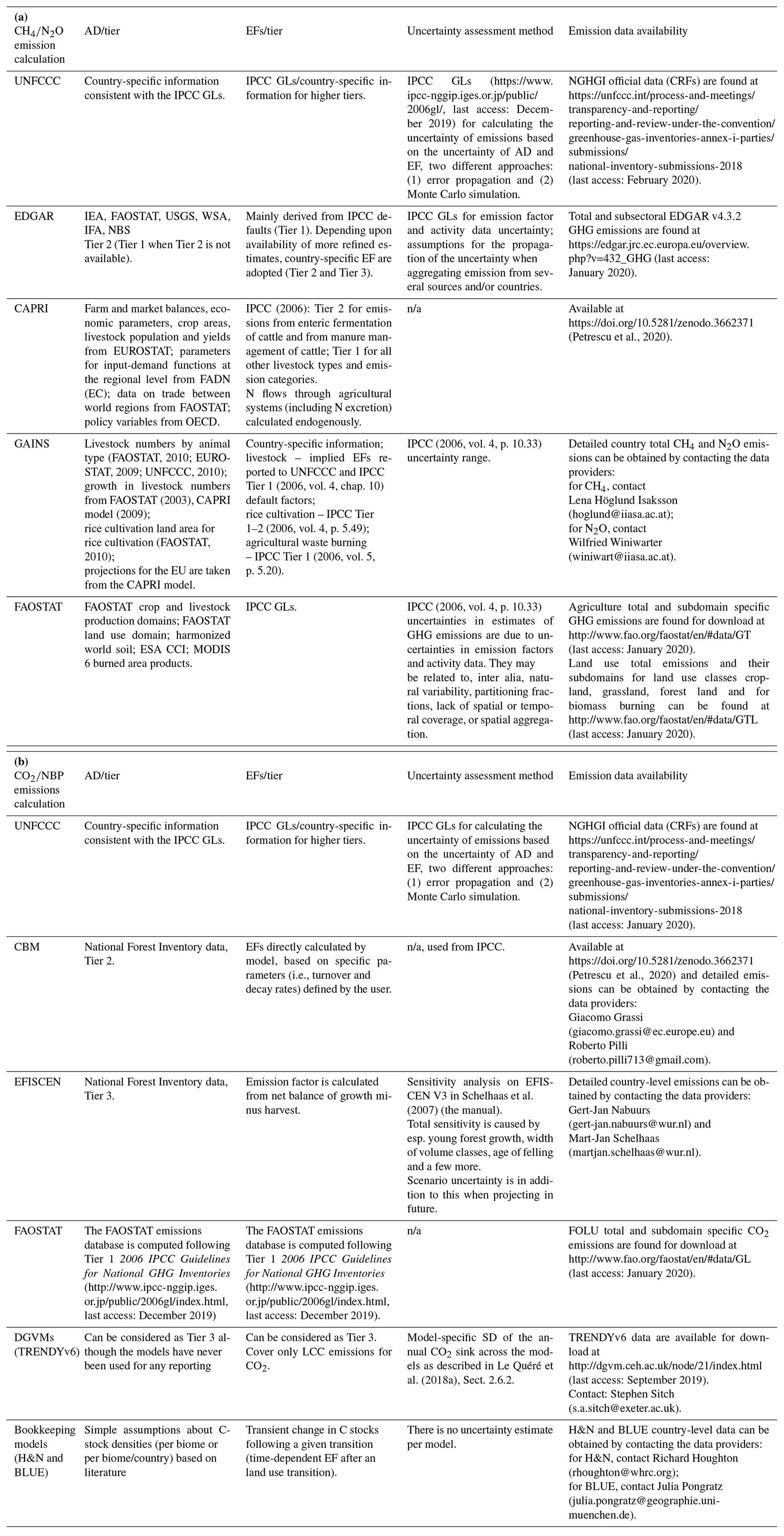
Table A2 Total EU28 agriculture and LULUCF estimates in kilotons of gas per year reported by the five data sources for the last available year (in bold).

Appendix B: Data source description

B1 UNFCCC

The UNFCCC committed in articles 4 and 12 in particular developed country parties listed in the Annex I of the UNFCCC to provide a national inventory of anthropogenic emissions by sources and removals by sinks of all GHGs not controlled by the Montreal Protocol using comparable methodologies. The Conference of the Parties (COP) decided in 2013 (Decision 24/CP.19⁸) on the Revision of the UNFCCC reporting guidelines on annual inventories for Parties included in Annex I to the Convention (UNFCCC 2013), hereafter UNFCCC reporting GLs, based on the 2006 IPCC Guidelines for National GHG Inventories (Eggleston et al., 2006). Developing countries are neither requested to mitigate GHG emissions nor requested to provide detailed information on national GHG emissions on an annual basis.

The exclusion of developing countries is explained by the fact that in the 1990s, when the Convention's and the Kyoto Protocol's reporting system was developed and adopted, a clear division of the regional distribution of GHG emissions existed. In industrialized countries, most GHG emissions were released, while in developing and emerging countries, emissions were low (Berger et al.. 2016).

The UNFCCC reporting guidelines decided to commonly use the global warming potentials (GWP)⁹ values with a 100-year horizon of the IPCC Fourth Assessment Report (IPCC, 2007) for the calculation of emissions in order to compare different GHG and to report the emission in complete time series from 1990 up to 2 years before the due date of the reporting, using the spreadsheets of the common reporting format (CRF). The reporting is strictly source category based and divided into the following main sectors: energy (CRF 1); industrial processes and product use (CRF 2); agriculture (CRF 3)¹⁰; land use, land use change, and forestry (LULUCF) (CRF 4)¹¹; and waste (CRF 5). For each sector, the CRF tables of the UNFCCC reporting guidelines provide a detailed catalog of source categories reflecting a comprehensive inventory of all sources and sinks of the abovementioned gases within an economy. Together with the calculation and reporting of emissions by sources and removals by sinks, countries have to provide a mandatory assessment of the uncertainties of the data provided.

Chapter 3 of the 2006 IPCC Guidelines for National GHG Inventories on the mandatory uncertainty assessment provides two approaches for the uncertainty calculations in NGHGIs:

1. error propagation;

2. Monte Carlo simulations.

For both approaches chap. 3 uses two main statistical concepts – the probability density function (PDF) and confidence limits, where the probability density function describes the range and relative likelihood of possible values and the confidence limits give the range (confidence interval) within which the underlying value of an uncertain quantity is thought to lie for a specified probability.

Under Approach 1, there are two ways in which uncertainties can be calculated.

• a.

  Where uncertain quantities are to be combined by multiplication, the standard deviation of the sum will be the square root of the sum of the squares of the standard deviations of the quantities that are added.

• b.

  Where uncertain quantities are to be combined by addition or subtraction, the standard deviation of the sum will be the square root of the sum of the squares of the standard deviations of the quantities that are added.

For this study an analysis of the reported uncertainties under the NGHGI for CO₂, CH₄ and N₂O has been performed for 26 EU countries¹². The analysis has not been performed for Sweden and the Czech Republic due to lack of data (e.g., confidential data). Due to lack of data availability only Approach 1 – propagation of error – has been applied to each country's uncertainty assessment in order to identify the main uncertainties. The second approach (i.e., Monte Carlo simulations) was not used in this study, although it presumably provided the more meaningful results.

Since the EU MS all report on different subsectors, the uncertainties have been aggregated to the subsectors per gas that all countries have in common; see the following Table B1¹³.

Table B1 Aggregation of subsectors for the uncertainty analysis.

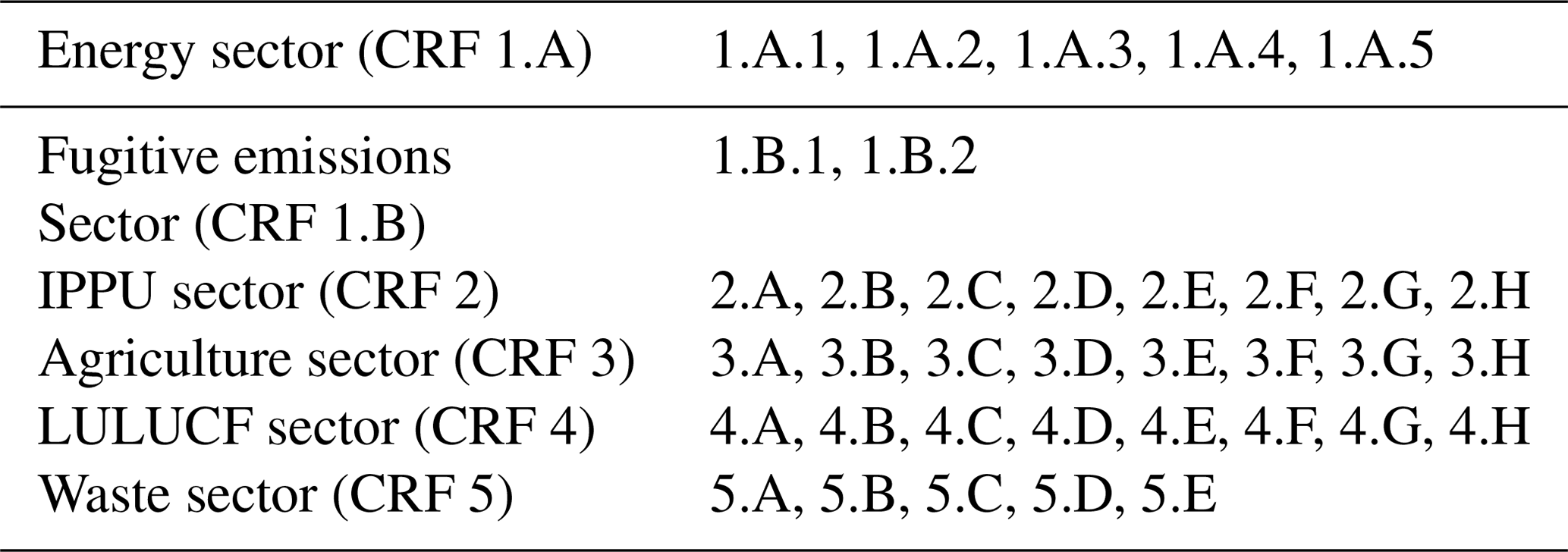
Generally, for almost all countries, the uncertainties for CO₂, CH₄ and N₂O in the agriculture sector and LULUCF sector are rather high and variable compared to the other sectors. For the EU as a whole, the uncertainties vary by sector; for the agriculture sector it is 45.4 %, and for the LULUCF sector it is 33 % (UNFCCC, 2018). This is because of the inherently different aspects of these sectors due to their dependencies on a number of variable factors and parameters, which make it harder to measure GHGs accurately. For example, Rypdal and Winiwarter (2001) claim that it is the incomplete understanding of soils that is the largest contribution to national uncertainty assessments, which can be confirmed with the uncertainty analysis¹⁴.

B2 EDGAR

The Emissions Database for Global Atmospheric Research (EDGAR) with versions EDGARv4.3.2 and EDGAR FT2017 provide global, country-level and gridded annual emissions of CO₂, CH₄ and N₂O (as well as of other species, not discussed here), used by policy makers and the IPCC (AR5).

EDGAR is developed and maintained by the Joint Research Centre of the European Commission, with continued inputs by PBL. The version v4.3.2 released in 2017, Janssens-Maenhout et al. (2019), provides 0.1^∘ gridded emissions from 1970 to 2012. The fast track (FT) version produced every year using a variant method provides time series updates making use of the latest available information on major sources (energy statistics of IEA and BP).

The EDGAR v4.3.2FT2015 has been producing 2015 grid maps at ${\mathrm{0.1}}^{\circ }\times {\mathrm{0.1}}^{\circ }$ resolution for the H2020 project CO₂ human emissions (CHE). The agriculture component of EDGAR comprises the agricultural soils (crops that are not rice) (N₂O), application of urea and agricultural lime (N₂O), enteric fermentation (CH₄), rice cultivation (CH₄), manure management (CH₄, N₂O), fertilizer use (synthetic and manure) (N₂O) and agricultural waste burning (in field) (CH₄, N₂O), and it is based on agricultural statistics and commodity statistics for some products (e.g., lime). Although agricultural field burning is included, other large-scale biomass burning from Savannah and forests and carbon stock changes due to land use activities are not included in EDGAR (Janssens-Maenhout et al., 2019). Details on EDGAR methodology for emissions calculations and uncertainties are referenced in Table A1a. Recently, EDGAR v4.3.2FT2015 has been updated to EDGAR v5/v4.3.2FT2017 (Olivier and Peters, 2018), which includes national CH₄ and N₂O emissions up to 2017.

EDGAR uses emission factors (EFs) and activity data (AD) to estimate emissions. Both EFs and AD are uncertain to some degree, and when combined their uncertainties need to be combined too. To estimate EDGAR's uncertainties (stemming from lack of knowledge of the true value of the EF and AD), the methodology devised by IPCC (2006, chap. 3) is adopted, that is, the sum of squares of the uncertainty of the EF and AD (uncertainty of the product of two variables). When aggregating the emissions from subcategories, or different sources, or countries the covariance of the respective probability distribution enters into play.

The assumptions introduced by Bond et al. (2004), Bergamaschi et al. (2015) and Olivier et al. (2002) hold:

• uncertainties of different source categories are uncorrelated;

• subsectors for CH₄ and N₂O are fully correlated; thus the uncertainty of the sum is the sum of the uncertainties;

• when dealing with CO₂, full correlation is assumed for subsets sharing the same emission factors (typically fuel-dependent); and

• aggregated emissions from same categories but different countries assume full correlation, unless the emission factor is country-specific or derived from higher tiers (i.e., not default EF defined by IPCC).

In addition, the following assumption is adopted:

• When uncertainty is defined within a range (e.g., for the energy sector, IPCC recommends that the methane emission factors are treated with an uncertainty ranging from 50 % to 150 %), the upper bound of the range is assigned to developing countries, while the lower bound is assigned to developed countries. Uncertainty of country or process-specific EF is not propagated (no correlation).

Table B2 Uncertainty assigned to activity data (AD) and emission factors (EF) for CH₄ and N₂O. The table is mostly derived by IPCC GLs (IPCC, 2006) for Tier 1 emission factors, complemented with estimates by Olivier et al. (2002) and expert judgment.

I: industrialized (developed) countries; D: developing countries; CS: country-specific.

Although assuming full correlation when aggregating emissions is quite conservative (overestimating the uncertainty introduced by emission factors), this approach is intended to balance other sources of uncertainty that are not taken into account, such as covariance among activity data (deemed negligible); uncertainty of technology factors (no information available as to how these factors are uncertain, as for example on the different rice cultivar practices); and uncertainty due to the fast track, i.e., applying trends to estimate latest year's emissions.

The EFs and AD uncertainties are reported in Table B2.

A lognormal probability distribution function is assumed to avoid negative values, and uncertainties are reported as 95 % confidence intervals according to IPCC (2006, chap. 3, Eq. 3.7). For emission uncertainty in the range 50 % to 230 % a correction factor is adopted as suggested by Frey et al. (2003) and IPCC (2006, chap. 3, Eq. 3.4). The correction factor is used as an empirical adjustment, based on Monte Carlo simulations, to correct for the deviation introduced by using the standard uncertainty calculation method suggested by IPCC error propagation, which is only a first-order approximation; for large uncertainties (as they accumulate in the propagation chain) the method systematically underestimates the uncertainty half range.

B3 CAPRI

CAPRI is an economic, partial equilibrium model for the agricultural sector, focused on the EU (as well as less detailed worldwide for market module) (Britz and Witzke, 2014¹⁵; Weiss and Leip, 2012¹⁶). CAPRI stands for Common Agricultural Policy Regionalised Impact Modelling System, and the name hints at the main objective of the system: assessing the effect of Common Agriculture Policy (CAP) instruments not only at the EU or member state level but at the subnational level. The model is calibrated for the base year (currently 2012), and then baseline projections are built, allowing the ex ante evaluation of agricultural policies and trade policies on production, income, markets, trade and the environment. It runs at a yearly time step at NUTS2 resolution but can be downscaled at the HSU level (approx. 1 km × 1 km). A detailed description can be found at https://ec.europa.eu/clima/sites/clima/files/strategies/analysis/models/docs/capri_model_methodology_en.pdf (last access: September 2019).

Among other environmental indicators, CAPRI simulates CH₄ and N₂O emissions from agricultural production activities (enteric fermentation, manure management, rice cultivation, agricultural soils). Activity data are mainly based on FAOSTAT and EUROSTAT statistics and estimation of emissions follows IPCC (2006) methodologies, with a higher or lower level of detail depending on the importance of the emission source. Details on CAPRI methodology for emissions calculations are referenced in Table A1a.

B4 FAOSTAT

FAOSTAT (Statistics Division of the Food and Agriculture Organization of the United Nations) CO₂, CH₄ and N₂O emissions from agriculture and LULUCF statistics until 2017 are available at http://www.FAOSTAT.org/FAOSTAT/en/#home (last access: January 2020). The FAOSTAT emissions database is computed following Tier 1 2006 IPCC Guidelines for National GHG Inventories (http://www.ipcc-nggip.iges.or.jp/public/2006gl/index.html, last access: December 2019). Country reports to FAO on crops, livestock and agriculture use of fertilizers are the source of activity data. Forest data are those reported to FAO within the FRA process. Geospatial data are the source of AD for the estimates from cultivation of organic soils, biomass and peat fires. GHG emissions are provided by country, regions and special groups, with global coverage, relative to the period 1961–present (with annual updates) and with projections for 2030 and 2050, expressed as Gg CO₂ and CO₂ eq. (from CH₄ and N₂O), by underlying agricultural emission subdomain and by aggregate (agriculture total, agriculture total plus energy, agricultural soils). Similarly, “land use total contains all GHG emissions and removals produced in the different land use subdomains, representing the three IPCC land use categories: cropland, forest land, and grassland, collectively called emissions/removals from the LULUCF sector. LULUCF emissions consist of CO₂ (carbon dioxide), CH₄ (methane) and N₂O (nitrous oxide) associated with land management activities. CO₂ emissions/removals are derived from estimated net carbon stock changes in above- and belowground biomass pools of forest land, including forest land converted to other land uses. CH₄ and N₂O, as well as additional CO₂ emissions, are estimated for fires and drainage of organic soils” (http://www.fao.org/faostat/en/#data/GL/metadata, last access: December 2019).

B5 GAINS

The Greenhouse Gas and Air Pollution Interactions and Synergies (GAINS) model (http://gains.iiasa.ac.at/, last access: September 2019) provides a framework for assessing strategies that reduce future emissions of multiple air pollutants and GHGs at lower costs and minimize their negative effects on human health, ecosystems and climate change. Although the focus of GAINS is more on future scenarios and air quality policies, GAINS estimates for its baseline historical emissions from 1990 to 2050 of 10 air pollutants and 6 GHGs for each country based on data from international energy and industrial statistics, on emission inventories, and on data supplied by countries themselves. It assesses emissions on a medium-term time horizon, with projections being specified in 5-year intervals through the year 2050 for N₂O and at a yearly time step for CH₄ (http://www.iiasa.ac.at/web/home/research/researchPrograms/air/GAINS.html, last access: September 2019). An important objective of the GAINS model is to use a consistent emission estimation methodology across all countries and sectors. Country- and sector/technology-specific emission factors are often derived in a consistent manner and are known to influence emissions, thereby producing emission estimates that are comparable across geographic and temporal scales and for which it is possible to explain deviations in emissions. By identifying the impact on emissions from implementation of various control technologies, the GAINS model can assess the expected impact on emissions from introducing additional control in the future.

B6 CBM

The Carbon Budget Model developed by the Canadian Forest Service (CBM-CFS3) can simulate the historical and future stand- and landscape-level C dynamics under different scenarios of harvest and natural disturbances (fires, storms), according to the standards described by the IPCC (Kurz et al., 2009), under an annual time step. Since 2009, the CBM has been tested and validated by the Joint Research Centre of the European Commission (JRC) and adapted to the European forests. It is currently applied to 26 EU MS, both at the country and at the NUTS2 level (Pilli et al., 2016).

Based on the model framework, each stand is described by area, age, and land use classes, as well as up to 10 classifiers based on administrative and ecological information and on silvicultural parameters (such as forest composition and management strategy). A set of yield tables define the merchantable volume production for each species while species-specific allometric equations convert merchantable volume production into aboveground biomass at the stand level. At the end of each year the model provides data on the net primary production (NPP), carbon stocks and fluxes, as the annual C transfers between pools and to the forest product sector.

The model can support policy anticipation, formulation and evaluation under the LULUCF sector, and it is used to estimate the current and future forest C dynamics, both as a verification tool (i.e., to compare the results with the estimates provided by other models) and to support the EU legislation on the LULUCF sector (Grassi et al., 2018a). In the biomass sector, the CBM can be used in combination with other models to estimate the maximum wood potential and the forest C dynamic under different assumptions of harvest and land use change (Jonsson et al., 2018).

B7 EFISCEN

The European Forest Information SCENario Model (EFISCEN) is a large-scale forest model that projects forest resource development on a regional to European scale. The model uses National Forest Inventory data as a main source of input to describe the current structure and composition of European forest resources. The model runs for 5-year-interval emission projections and projects the development of forest resources, based on scenarios for policy, management strategies and climate change impacts. With the help of biomass expansion factors, stem wood volume is converted into whole-tree biomass and subsequently to whole-tree carbon stocks. Information on litter fall rates, felling residues and natural mortality is used as input into the soil model Yasso (Liski et al., 2005), which is dynamically linked to EFISCEN and delivers information on forest soil carbon stocks. The core of the EFISCEN model was developed by Ola Sallnäs at the Swedish Agricultural University (Sallnäs, 1990). It has been applied to European countries in many studies since then, dealing with a diversity of forest resource and policy aspects. A detailed model description is given by Verkerk et al. (2016), with online information on availability and documentation of EFISCEN at http://efiscen.efi.int (last access: September 2019). The model and its source code are freely available, distributed under the GNU General Public License conditions (http://www.gnu.org/licenses/gpl-3.0.html, last access: September 2019).

B8 DGVMs (TRENDY v6)

This study uses the ensemble of eight DGVMs that participated in TRENDY version 6 (v6) for the GCB 2017 (Le Quéré et al., 2018a) including the following models: ORCHIDEE (Krinner et al., 2005), OCN (Zaehle et al., 2011), JULES (Clark et al., 2011), JSBACH (Reick et al., 2013), VEGAS (Zeng 2003, 2005), LPX-Bern (Lienert and Joos, 2018), LPJ (Sitch, 2003) and ISAM (Jain et al., 2013). We make use of carbon trends in net land carbon exchange over Europe, during the period 1990–2016. Data are available for download at http://dgvm.ceh.ac.uk/index.html (last access: September 2019). DGVMs are forced by historical agricultural land cover change, climate change and CO₂ since 1901. The models calculate forest area from agricultural land in different ways and therefore can have quite different forest areas in the EU. Models include biomass and soil C loss or gains associated with land cover change and wood harvest (diagnosed from factorial simulations), but they do not include a realistic representation of cropland management for Europe or of forestry and grassland management. The time step of each of the models is described in detail in Le Quéré et al. (2018a), Table 4 and references therein.

B9 Bookkeeping models

The LULUCF chapter makes use of data from two bookkeeping models: H&N (Houghton and Nassikas, 2017) and BLUE (Hansis et al., 2015). As described by GCB 2017 (Le Quéré et al., 2018a), the H&N model (Houghton et al., 1983) calculates land use change CO₂ emissions and uptake fluxes for transitions between various natural vegetation types and agricultural lands (croplands and pastures). The original bookkeeping approach of Houghton (2003) keeps track of the carbon stored in vegetation and soils before and after the land use change. Carbon gain or loss is based on response curves derived from the literature. The response curves describe the decay of vegetation and soil carbon, including transfer to product pools of different lifetimes, as well as carbon uptake due to regrowth of vegetation and consequent refilling of soil carbon pools. Natural vegetation can generally be distinguished into primary and secondary land. For forests, a primary forest that is cleared cannot recover back to its original carbon density. Instead long-term degradation of primary forest is assumed and represented by lower standing vegetation and soil carbon stocks in the secondary forests. Apart from land use transitions between different types of vegetation cover, forest management practices in the form of wood harvest volumes are included. Different from dynamic global vegetation models, bookkeeping models ignore changes in environmental conditions (climate, atmospheric CO₂, nitrogen deposition and other environmental factors). Carbon densities at a given point in time are only influenced by the land use history but not by the preceding changes in the environmental state. Carbon densities are taken from observations in the literature and thus reflect environmental conditions of the last decades (Le Quéré et al., 2018a).

The BLUE model provides a data-driven estimate of the net land use change fluxes. BLUE stands for bookkeeping of land use emissions. Bookkeeping models (Hansis et al., 2015; Houghton et al., 1983) calculate land use change CO₂ emissions (sources and sinks) for transitions between various natural vegetation types and agricultural lands. The bookkeeping approaches keep track of the carbon stored in vegetation, soils, and products before and after the land use change.

In BLUE, land use forcing is taken from the Land Use Harmonization dataset, LUH2, for estimates within the annual global carbon budget. The model provides data at annual time steps and 0.25^∘ resolution. Temporal evolution of carbon gain or loss, i.e., how fast carbon pools decay or regrow following a land use change, is based on response curves derived from the literature. The response curves describe the decay of vegetation and soil carbon, including transfer to product pools of different lifetimes, as well as carbon uptake due to regrowth of vegetation and subsequent refilling of soil carbon pools.

B10 Wetland emissions ensemble of models

This model ensemble simulates natural CH₄ emissions from wetlands and contains 11 biogeochemical models (CLM4.5, Riley et al., 2011; CTEM, DLEM, Tian et al., 2010; VISIT, Ito and Inatomi, 2012; JULES, Hayman et al., 2014; LPJ-MPI, Kleinen at al., 2012; LPJ-wsl, Hodson et al., 2011; LPX-Bern, Spahni et al., 2011; ORCHIDEE, Ringeval et al., 2010; SDGVM, Hopcroft et al., 2011; TRIPLEX-GHG, Zhu et al., 2015). These models are referenced and can be found in the Poulter et al. (2017) Supplement: https://iopscience.iop.org/1748-9326/12/9/094013/media/ERL_12_9_094013_suppdata.pdf (last access: December 2019).

Appendix C: Example of country-specific uncertainty calculation for LULUCF sector 4

For a better understanding and overview of the single steps of the uncertainty analysis, an example calculation for the uncertainty assessment is included, where the combined uncertainty and contribution to variance is calculated for 4.A CO₂. The same was done for 4.B, 4.C, etc.

Table C1 Aggregation of IPCC subsectors for the uncertainty analysis.

Table C2 Calculation example of the uncertainty analysis; uncertainty assessment 2016.

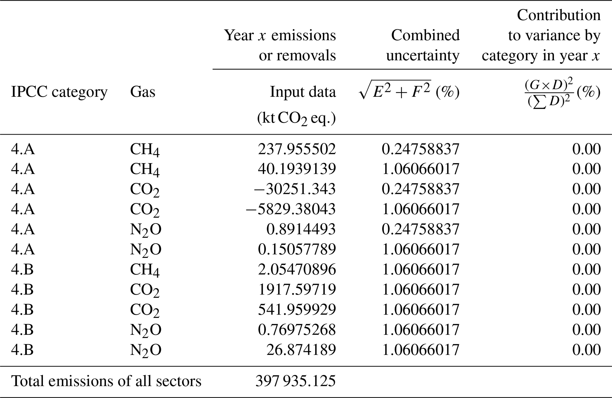
1. Table C2 shows the subsectors 4.A and 4.B of one the EU28 MS uncertainty assessments for 2016.

2. To calculate the contribution to variance for the sector 4.A CO₂, the following steps have to be performed:

   1. $(-\mathrm{30251},\mathrm{343})+(-\mathrm{5829},\mathrm{38})=(-\mathrm{36080},\mathrm{72})$ (building the sum of the emissions of year x for 4.A, CO₂);

   2. $\left(\right(-\mathrm{30251},\mathrm{343}\times \mathrm{0},\mathrm{24758837}{)}^{\mathrm{2}}+(-\mathrm{5829},\mathrm{38}\times \mathrm{1},\mathrm{06066017}{)}^{\mathrm{2}})/(-\mathrm{36080},\mathrm{72}{)}^{\mathrm{2}}=\mathrm{0},\mathrm{0724584}$ (intermediate step for calculating the combined uncertainty);

   3. $\text{SQRT}(\mathrm{0},\mathrm{0724584})=\mathrm{26},\mathrm{918}$ % (combined uncertainty);

   4. $\left(\right(-\mathrm{36080},\mathrm{7234}\times \mathrm{26},\mathrm{918}{)}^{\mathrm{2}})/\mathrm{397935},{\mathrm{125}}^{\mathrm{2}}=\mathrm{0},\mathrm{001}$ (contribution to variance for year x).

3. Results can be found in Table C3.

Table C3 Calculation example of the uncertainty analysis; section from one of the MS of the EU28 uncertainty assessment 2016.

To check for correctness, the total uncertainty for the aggregated sectors can be calculated. If the total uncertainty for the aggregated sectors matches the total uncertainty of the uncertainty assessment, the calculated uncertainties for the subsectors are correct. This was the case for all calculations performed for this analysis.

The results of the uncertainty analysis show a clear trend of the main uncertainties and gases across the analyzed 26 EU MS.

Appendix D: Country-specific emissions

Detailed agriculture CH₄ and N₂O emissions split in activities for all EU28 countries can be downloaded at https://doi.org/10.5281/zenodo.3662371 (Petrescu et al., 2020) and are found under the “Figures5,8_AppendixD_CH₄_N₂O_per_country_new” excel document.

Appendix E: Acronyms and abbreviations

AD	Activity data
AFOLU	Agriculture, forestry and other land use
AR	Assessment report
BP	The British Petroleum Company
CAPRI	Common Agricultural Policy Regionalised Impact Modelling System
CBM	Carbon Budget Model
CH4	Methane
CO2	Carbon dioxide
CAP	Common Agriculture Policy
CL	Cropland
CLM4.5	Community Land Model
COP	Conference of the Parties
CRF	Common reporting format
CTEM	The Canadian Terrestrial Ecosystem Model
DIC	Dissolved inorganic carbon
DG CLIMA	Directorate General for Climate Action (European Commission)
DGVMs (TRENDY)	Dynamic global vegetation models
DLEM	Dynamic land ecosystem model
DOC	Dissolved organic carbon
EDGAR	Emission Database for Global Atmospheric Research
EEA	European Environmental Agency
EF	Emission factor
EFISCEN	European Forest Information SCENario Model
EIT Parties	Economies in transition
ESA CCI	European Space Agency Climate Change Initiative
ETS	Emissions Trading System
EU28	European Union
EUROSTAT	European Statistical Office
FADN	Farm Accountancy Data Network
FAOSTAT	Food and Agriculture Organization of the United Nations
FL	Forest land
FOLU	Forestry and other land use
FRA	Global Forest Resources Assessment
GAINS	Greenhouse Gas and Air Pollution Interactions and Synergies model
GCP	Global Carbon Project
GCB	Global Carbon Budget
GHGs	Greenhouse gases
GHGI	Greenhouse gas inventory
GL	Grassland
GMB	Global Methane Budget
H2020	Horizon 2020 EU research and innovation program
ICOS	Integrated Carbon Observation System
IEA	International Energy Agency
IFA	International Fertilizer Association
IPCC	Intergovernmental Panel on Climate Change
IPCC GLs	IPCC Guidelines
IPCC SRCCL	IPCC Special Report on Climate Change and Land
IPPU	Industrial processes and product use
JRC	Joint Research Centre of the European Commission
JULES	The Joint UK Land Environment Simulator
KP	Kyoto Protocol

LCC	Land cover change
LPJ-MPI	Lund-Potsdam-Jena model – Max Planck Institute version
LPJ-wsl	Lund-Potsdam-Jena model – WSL version
LPX-Bern	Land surface Processes and eXchanges model of the University of Bern
LULCC	Land uses and land cover change
LULUCF	Land use, land use change and forestry
MODIS	Moderate Resolution Imaging Spectroradiometer
MS	Member states
N2O	Nitrous oxide
NBP	Net biome production
NBS	National Bureau of Statistics of China
NDCs	Nationally determined contributions
NEP	Net ecosystem production
NFI	National Forest Inventory
NGHGI	National Greenhouse Gas Inventory
NIRs	National Inventory Reports
NPP	Net primary production
NUTS2	Nomenclature of territorial units for statistics
OECD	Organisation for Economic Co-operation and Development
ORCHIDEE	Organising Carbon and Hydrology In Dynamic Ecosystems
PA	Paris Agreement
PBL	Planbureau voor de Leefomgeving (Netherlands Environmental Assessment Agency)
RF	Remaining forestry
SBSTA	Subsidiary Body for Scientific and Technological Advice
SDGVM	Sheffield Dynamic Global Vegetation Model
SOC	Soil organic carbon
TACCC	Transparency, accuracy, consistency, completeness and comparability
TRIPLEX-GHG	A hybrid, monthly-time-step model of forest growth and carbon dynamics coupled with
	a new methane (CH4) biogeochemistry module
UNEP	United Nations Environment Programme
UNFCCC	United Nations Framework Convention on Climate Change
USGS	United States Geological Survey
VERIFY	Verifying greenhouse gas emissions, EU H2020 project, grant agreement no. 776810
VISIT	Vegetation Integrative Simulator for Trace Gases
VOC	Volatile organic compounds
WSA	World Steel Association
WWII	World War II