the Creative Commons Attribution 4.0 License.
the Creative Commons Attribution 4.0 License.
 | 14 Apr 2020
Disdrometer measurements under Sense-City rainfall simulator
Philippe Bruley
Anne Ruas
Daniel Schertzer
Ioulia Tchiguirinskaia
The Hydrology, Meteorology and Complexity Laboratory of École des Ponts ParisTech (http://hmco.enpc.fr, last access: 24 March 2020) and the Sense-City consortium (http://sense-city.ifsttar.fr/, last access: 24 March 2020) made available a dataset of optical disdrometer measurements stemming from a campaign that took place in September 2017 under the rainfall simulator of the Sense-City climatic chamber, which is located near Paris. Two OTT Parsivel2 disdrometers were used. The size and velocity of drops falling through the sampling area of the devices of roughly a few tens of square centimetres are computed by disdrometers. This enables the estimation of the drop size distribution and the further study of rainfall microphysics or kinetic energy for example. Raw data – basically a matrix containing a number of drops according to classes of size and velocity, along with more aggregated ones such as rain rate and drop size distribution with filtering – are available. The dataset is publicly available at https://doi.org/10.5281/zenodo.3347051(Gires et al., 2019).
- Article
(1692 KB) - Full-text XML
- BibTeX
- EndNote


Numerous rainfall simulators have been developed and used primarily to study soil erosion as well as tillage techniques. Indeed the natural extreme variability of rainfall features (e.g. occurrence, intensity, duration, drop size distribution), makes such study under natural conditions more complicated. For a short historical review of rainfall simulators and their uses, the interested reader is referred to Hall (1970). Rainfall simulators exhibit a wide range of complexity in terms of functioning enabling to reproduce more or less the properties of rainfall features depending on the aim of the study and the means available. Systems range from simple ones made of a network of few nozzles of various complexity (Olayemi and Yadav, 1983; Auerswald et al., 1992; Humphry et al., 2002; Paige et al., 2004; Parsons et al., 1998) to ones using disc-type water distributor hypodermic tube and needles in an attempt to reproduce not only a more or less uniform rainfall but also drop size distribution (DSD) and fall velocity of drops (Abd Elbasit et al., 2010).
Some authors analysed the rain simulated with the help of disdrometers, which are devices that give access to size and velocity of the falling drops. For example Meshesha et al. (2016) used such a set-up to investigate the relation between kinetic energy (KE) and rain rate (R), while Salles and Poesen (2000) showed that D4V (where D is the diameter of drops and V their velocity) was a better indicator for characterizing splash detachment than KE, which is basically proportional to D3V2. Iserloh et al. (2012) upgraded a portable rain simulator to investigate in detail the processes of runoff generation and erosion.
In this paper we present disdrometer data collected during a measurement campaign aiming at testing a rainfall simulator installed in the climatic chamber of the Sense-City experiment. The campaign took place in September 2017. Before continuing, it should mentioned that the two disdrometers used here are already presented in Gires et al. (2018a), which deals with a previous outdoor campaign involving other instruments as well. Hence only the required basic elements on their functioning will be mentioned here, while the reader is referred to the previous paper for more details as well as a longer discussion on the potential uses of such data. To the knowledge of the authors, such disdrometer data of rainfall simulators are not available to the community.
Data and methods are presented in Sect. 2 with a brief overview of the device functioning and available datasets as well a description of the rainfall simulator and the measurement campaign. Section 3 presents the database and the available tools to use it. Outputs of the campaign are discussed in Sect. 4 along with an illustrative comparison with some actual rainfall.
2.1 Brief reminder of the disdrometer functioning and available datasets
As pointed out in the introduction, the measurement campaign uses devices whose functioning has already been described in detail in Gires et al. (2018a). Hence only a short summary is given in this paper. The two devices are part of the TARANIS Observatory (exTreme and multi-scAle RAiNdrop parIS Observatory) (Gires et al., 2015, 2018a, b) of the Fresnel Platform of École des Ponts ParisTech (https://hmco.enpc.fr/portfolio-archive/fresnel-platform/ich, last access: 24 March 2020). The two optical disdrometers used here are OTT Parsivel2 (see Loffler-Mang and Joss, 2000; Battaglia et al., 2010; or the device documentation OTT, 2014), which are occlusion ones. It means that they are made of a transmitter, which generates a laser sheet and a receiver aligned with the transmitter with a sampling area of 54 cm2 in between. When a drop falls through it, the beam is partially occluded, which results in a decrease of the signal reaching the receiver. The amplitude and the duration of the decrease in the received signal are then analysed to estimate the equivolumic diameter and the velocity. If two drops fall through the sampling area at exactly the same time (which is a very rare event given typical drop concentration), they will be computed as a larger drop with an unexpected velocity, which can help remove the measurement.
The output provided is actually not directly the features of each individual drop but rather a matrix containing the number of drops recorded during the time step Δt (here Δt=30 s) according to classes of equivolumic diameter (index i and defined by a centre Di and a width ΔDi expressed in mm) and fall velocity (index j and defined by a centre vj and a width Δvj expressed in m s−1). The classes are listed in Table 1.
Table 1Definition of the classes of particle size and velocity for the Parsivel2.
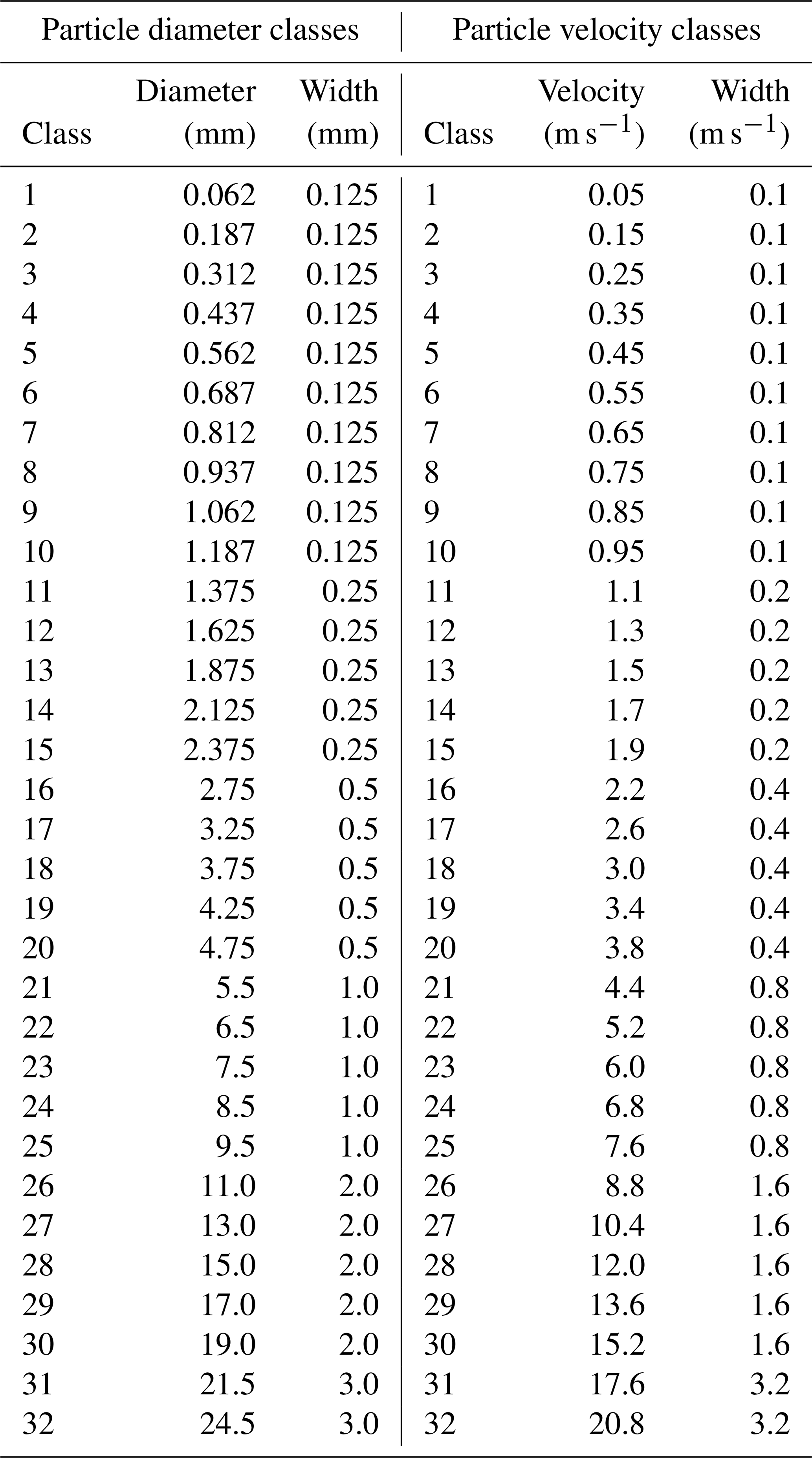
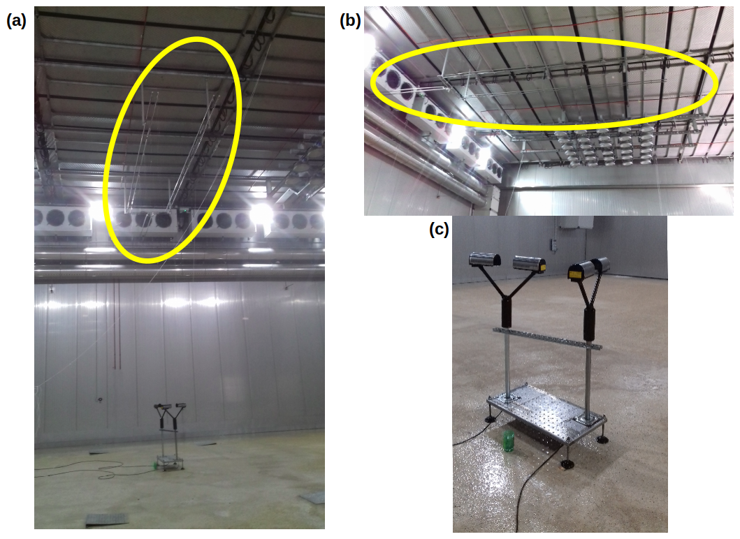
Figure 1Pictures showing an overview of the measurement campaign (a), a zoom on the rainfall simulator (b), and the disdrometers (c). The rainfall simulator, with its two separate networks for light and heavy rainfall, is indicated in yellow.
The three quantities analysed in the paper and made available in the corresponding database are the rain rate R in millimetres per hour, the drop size distribution N(D) per cubic metre per millimetre (N(D)dD is the number of drops per unit volume in cubic metres with an equivolumic diameter between D and D+dD in mm), and the kinetic energy density flux KE in joules per square metre per hour. Equivalently, we could have worked on a “kinetic energy” expressed per millimetre of rain (i.e. in KE in J m−2 mm−1), which is simply equal to KE∕R (see Angulo-Martínez and Barros, 2015, for a discussion on the use of both). The studied quantities are obtained for each time step from the raw matrix with the help of the following expressions:
where Seff(Di) is the sampling area of the device. In the data presented in the paper for the Parsivel2, we used , where L=180 mm and W=30 mm are the length and width of the sampling area, respectively (LW=54 cm2) (OTT, 2014). Since there is no modification on the raw data, the user can choose other approaches. It is a discrete DSD N(Di) that is computed, in which N(Di)ΔDi gives the number of drops with a diameter in the class i per unit volume (in m−3). ρwat=103 kg m−3 is the volumic mass of water.
Finally it should be mentioned that no filter was implemented on the matrix for this specific implementation; i.e. the whole matrix is used. In some case authors introduced a filter to exclude drops whose measured fall velocity was too far from the theoretical expected terminal fall velocity and hence assumed to correspond to non-meteorological hydrometeors (Gires et al., 2018a; Thurai and Bringi, 2005; Jaffrain and Berne, 2012). Again, since the raw matrices are made available, users can choose to implement a filter if they want.
2.2 Description of the rainfall simulator
Sense-City is a 400 m2 climate chamber funded by the French Research Agency. It allows the programming of climate (temperature and humidity) as well as sun and rain. A tiny city is built inside the climate chamber to study different components of the city. The main research subjects are nanosensor and microsensor conception, air and water pollution, energy, and the impact of materials and vegetation on climate and pollution in different climates.
The rainfall simulator does not cover all the areas but only a 25 m2 rectangular portion (3 m × 8.3 m; see Fig. 1). Two modes of rain are available: light and heavy rain. Each of them is produced by different injection nozzles. These nozzles are characterized through the angle of their internal cone. The manufacturer installed 12 nozzles with an angle of 90∘ for light rain and 12 nozzles with an angle of 120∘ for heavy rainfall. The nozzles for each type of rain are distributed over two separate systems basically made of a “fork” pipe each. The location of the nozzles and lines of nozzles are shown in Fig. 2. The nozzles are located at 8 m height. The water flow can vary from 7 to 14 L min−1 for light rain and from 11 to 20 L min−1 for heavy rain. The water flow is fixed for each simulation and is not supposed to vary more than 2 %. The water used is drinking water.
2.3 Measurement campaign
The measurement campaign took place 26–28 September 2017 in the Sense-City climatic chamber. Some pictures illustrating it can be found in Fig. 1. An overview of the set-up is visible in Fig. 1a, where the area normally covered by the rainfall simulator is identified by four metallic squares. The rainfall simulator, with its two separate networks for light and heavy rainfall, is highlighted in yellow. A zoom of the rainfall simulator and the two disdrometers used can be found in Fig. 1b and c, respectively .
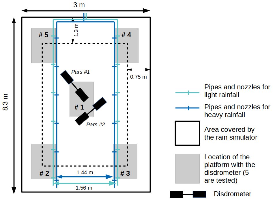
Figure 2Scheme of the various locations tested over the area covered by the rainfall simulator.
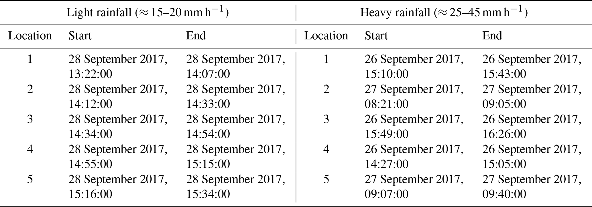
Measurements were carried out for both light and heavy rainfall at five different locations within the area wet by the rainfall as shown in Fig. 2. The precise timing in local time of each test can be found in Table 2. Each test lasted at least 15 min. It takes a few minutes at the beginning to reach a steady state.
In addition, a specific test keeping the disdrometers at location no. 1 while changing the input flow of water was carried out on 27 September 2017 between 09:45:00 and 11:20:00. Given that the rainfall simulator is not designed for such use, it resulted in a malfunctioning of the nozzles, notably with very large drops falling on the wet area. Hence measurement during this period is not discussed in this paper and should not be considered.
Table 2Start and end time of tests for each location in both light and heavy rainfall configuration. Local time is used.
This section is actually quite similar to the corresponding one of Gires et al. (2018a). It contains a description of the database content along with some available scripts. The dataset for this campaign can be found at https://doi.org/10.5281/zenodo.3347051 (Gires et al., 2019). The main differences are the addition of the computation of KE and changes in the calendar, which does not provide links to daily data but to individual tests. The database is organized as follows:
-
disdrometers_data_base/
-
Raw_data_zip/
-
Pars1/
-
Pasr2/
-
Each folder contains the files for its
disdrometers. -
The name is
Raw_DisdroName_YYYYMMDD.zip
(e.g. Raw_pars1_20170926.zip).
-
-
Daily_data_python/
-
Pars1/
-
Pasr2/
-
Each folder contains the files for its
disdrometers. -
The name is
DisdroName_raw_data_YYYYMMDD.csv
(e.g. Pars1_raw_data_20170926.npy).
-
-
Exports/
-
Full_matrix/
-
KE/
-
R/
-
Each folder contains the files for all the
disdrometers. -
The name is DisdroName_DataType_date.csv
(e.g. Pars1_KE_30_sec_2017_09_26_00_00_
00__2017_09_26_23_59_30).
-
-
Calendars/
-
Data_5_min/ (one file per day;
e.g. R_5_min_Sense_ City_2017_09_26_00_
00_00__2017_09_26_23_59_30.csv -
Data_30_sec/ (one file per day;
e.g. R_30_sec_Sense_City_2017_09_26_00_
00_00__2017_09_26_23_59_30.csv) -
Quicklooks/ (one file per day and test;
e.g. Quicklook_Sense_City_2017_09_26_00_
00_00__2017_09_26_23_59_30.png) -
Calendar_Sense_City.html
-
-
Python_scripts/
-
It contains the Python scripts (and associated
files) to generate and use this database.
-
-
Read_me.txt
-
It contains a short description of the Taranis
Sense-City database.
-
-
3.1 “/Calendars”
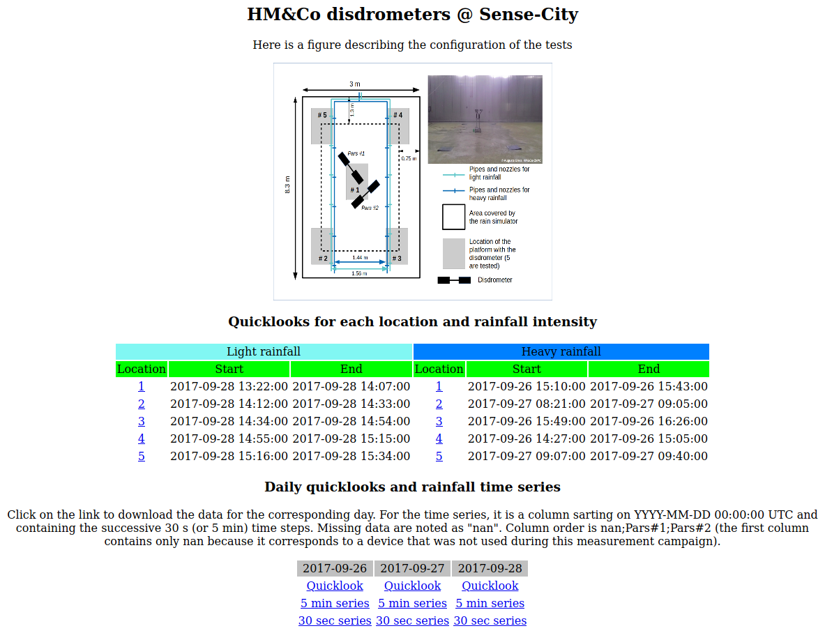
Figure 3 displays a snapshot of the page “Calendar_Sense_City.html” of the database. It summarizes the campaign and gives access to quicklooks of the measurements for each location and rainfall intensity. These quicklooks can also be directly accessed in the folder Quicklooks/. It also enables access to the daily quicklooks for each day (there are obviously numerous missing data, since disdrometers were only turned on during the actual tests), as well as of the corresponding rainfall times series with 30 s and 5 min time steps. These files can also directly be accessed in the folders Data_30_sec/ and Data_5_min/.
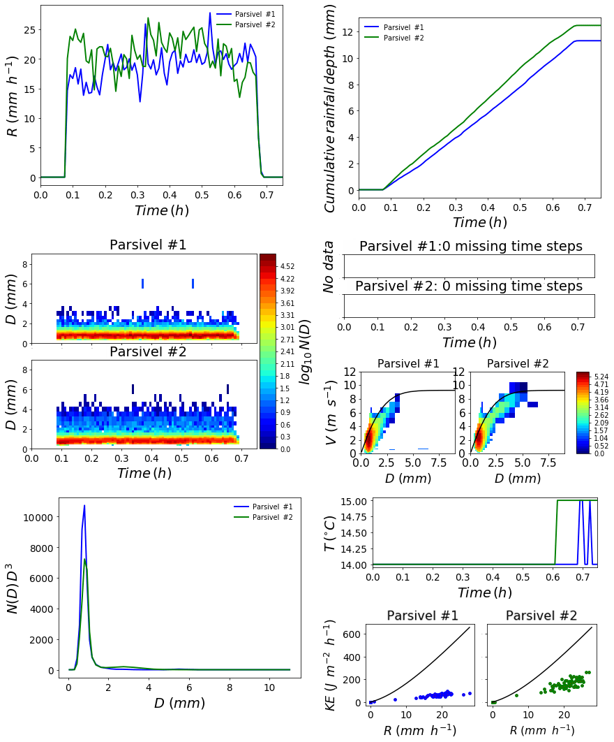
An example of quicklook can be found in Fig. 4, which is plotted for the test in location no. 1 with light rainfall. It aims at providing the user with an overview of the test. Quicklook's file names contain the name of the measurement campaign as well as the date and time of the start and end of the period it is covering. For example the file displayed in Fig. 4 is called “Quicklook_Sence_City_2017_09_28_13_22_00__2017_09_28_
14_07_00.png”, which means that it corresponds to the quicklook of “Sense-City” campaign between 28 September 2017 at 13:22:00 and 28 September 2017 at 14:07:00.
A quicklook contains the following graphs:
-
the rain rate R (in mm h−1) vs. time (in h) (upper left);
-
cumulative rainfall depth C (in mm) vs. time (in h) (upper right);
-
the DSD N(D) (in m−3 mm−1) vs. time (in h) (middle left);
-
time series of missing time steps (a visible coloured bar for missing ones) (middle right);
-
a visual representation of the matrix containing the number of drops according the velocity and size classes, with the classes of velocity represented vertically or diameter represented horizontally; the solid black line is the curve corresponding to the relation between the terminal fall velocity of drops as a function of their equivolumic diameter obtained by Lhermitte (1988) (middle right). It should be mentioned that only drops with a diameter smaller than 9 mm and a velocity smaller than 12 m s−1 are displayed, while larger and faster hydrometeors can be computed (see Table 1). This range, adapted to the typical features of rain drops, was chosen to improve visibility of the figure. The data provided contain all the information (actually in this case no drops outside of the display range);
-
N(D)D3 vs. D (lower left, N(D)D3 and not simply N(D) was plotted because it is proportional to the volume of rain obtained according to the drop diameter hence providing the reader a greater immediate insight of the contribution of each diameter class of drops to the observed rainfall amounts);
-
the temperature T (in ∘C) vs. time (in h);
-
the kinetic energy density flux KE (in J m−2 h−1) vs. the rain rate R (in mm h−1). The solid line corresponds to a standard relation for rainfall found in Angulo-Martínez and Barros (2015).
The files for daily rainfall rate are named in a similar way as the quicklooks except that “Quicklook” is replaced by “R_5_min” or “R_30_sec”. They are CSV files with the following format:
-
(i) There is one line per time step (either 30 s or 5 min time step starting on YYYY-MM-DD 00:00:00 LT).
-
(ii) In each line, values of rain rate (in mm h−1) during this time step for the two disdrometers are separated by a semicolon and are preceded by “nan”; (actually corresponding to a disdrometer not used in this campaign), and the order is nan;Pars#1;Pars#2.
-
(iii) Missing data are denoted by “nan”.
3.2 “/Exports”
This folder contains exports in a simple CSV format of the main outputs of the disdrometer that could be relevant for potential users of these data, i.e. the full matrix of drops according to size and velocity classes (subfolder “/Full_matrix”), kinetic energy density flux (subfolder “/KE”), and rain rate (subfolder “/R”).
In a given folder, a file is typically called “Pars1_KE_30_sec_2017_09_26_00_00_00__2017_09_26_
23_59_30.csv”, meaning the disdrometer name, the data type, and start and end of the period corresponding to the data are easily visible for the user. In the file, the format is the following: (i) one line per time step; (ii) for each line, date (YYYY-MM-DD HH:MM:SS); data. For R and KE data are simply the value for the corresponding time step. For the “full matrix” it is as follows: number of drops per class of velocity and size (1st size class – 1st velocity class, 1st size class – 2nd velocity class, 1st size class – 2nd velocity class, …, 2nd size class – 1st velocity class …) separated by commas (32×32 classes for Parsivel data). Here is an example: 26 September 2017 17:27:00; 0.0,0.0,0.0…,0.0. (iii) Missing data are indicated by nan. These files are text files that can be read by any software.
3.3 “/Daily_data_python”
This folder contains the daily file for both disdrometers in their own subfolder. Each file is stored in NPY format and requires Python 3 to be read. They contain all the collected data stored as a list. It is these files that are read by the Python scripts described in the corresponding subsection.
3.4 “/Raw_data_zip”
This folder is actually very similar to the corresponding one of Gires et al. (2018a), so the description will simply be repeated: “It contains a folder for each of the three disdrometers. Each of these folders contains a zip file for each day. This .zip file contains the data directly collected from the disdrometer. There is one text file for each 30 s time step. The precise format of these fields can be found in the Python scripts in the heading of the corresponding functions. This corresponds to the raw data. These data have been made available for expert users, but in practice it is believed that the .csv file or the Python scripts should be sufficient for most users.”
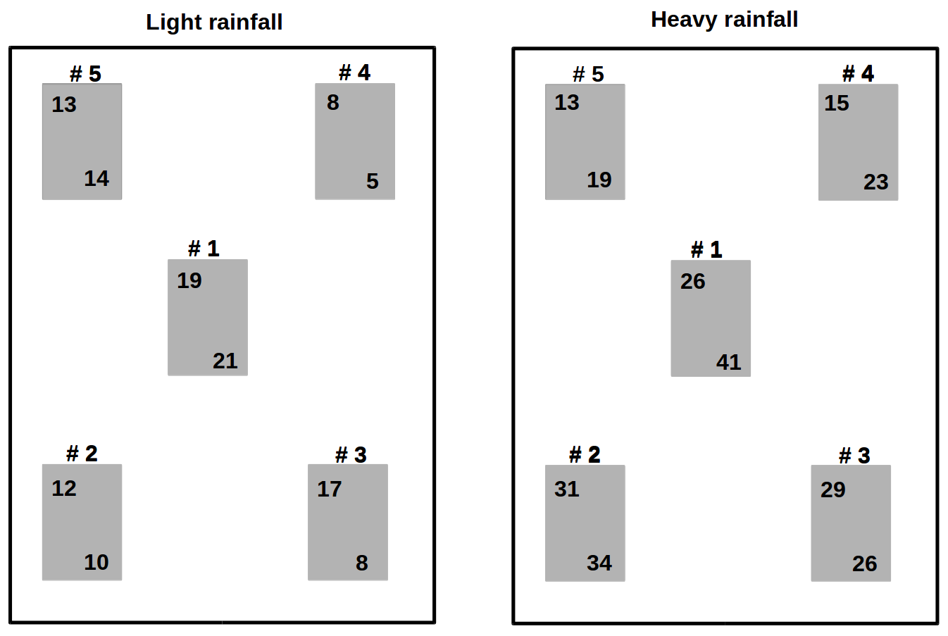
Figure 5Average rain rate expressed in millimetres per hour for each location (#) for both light and heavy rainfall simulations.
3.5 Python scripts/
Again this section is very similar to the corresponding one of Gires et al. (2018a), with the addition of the function to export KE. This folder contains some Python scripts that can be used to carry out some initial analysis and data treatment with the database. The tools are located in the script “Tools_data_base_use_Sense_City_v4.py”. The main functions are (only a short description is given here – more details, including precise description of the inputs and outputs of the functions, are provided as comments in each script):
-
Quicklook_and_R_series_generation_Sense_City_
without_PWS generates a quicklook image and the corresponding 30 s and 5 min rain rate time series for a given rainfall event for the Sense_City campaign. -
extracting_one_event_Sense_City reads daily.npy files and generates three lists (one for each disdrometer) containing all the data that can be analysed for the Sense_City campaign.
-
exporting_full_matrix reads daily NPY files and exports the full matrix in CSV files for a given disdrometer and event.
-
exporting_R readings daily NPY files and exports R in CSV files for a given disdrometer and event.
-
exporting_T reads daily NPY files and exports T in CSV files for a given disdrometer and event.
-
exporting_KE reads daily NPY files and exports KE in CSV files for a given disdrometer and event.
Commented examples of use of the functions can be found in the scripts: “Example_of_use_data_base_sense_city.py”. Note that Python 3 (https://www.python.org/, last access: 24 March) is required because the NPY files containing the data were saved using Python 3.
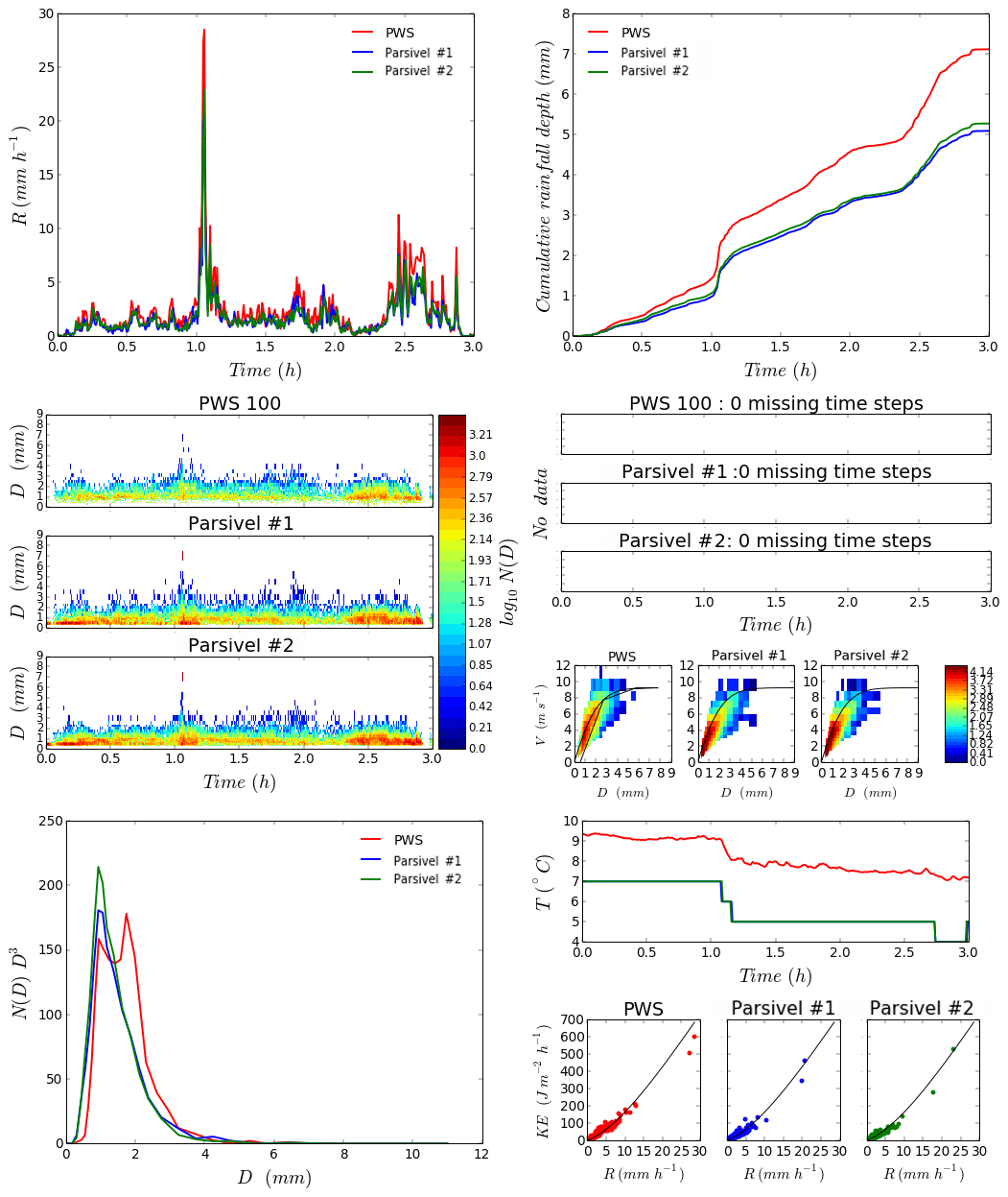
Figure 7Quicklook of the measurements carried out on the roof of the Carnot Building of ENPC campus on 10 February 2019 between 07:00:00 and 10:00:00 UTC.
4.1 Not homogeneous over the surface
Figure 5 displays the average rain rate expressed in millimetres per hour measured at each location (#) and disdrometer for both light and heavy rainfall simulations. The first and last 5 min were not considered in the computation of the average. It appears that for both rainfall configurations, the rain rate is not uniform over the wet surface. This phenomenon is more pronounced for heavy rainfall, with even a strong disparity between the two disdrometers at location no. 1 (see Fig. 6). In general and not surprisingly, there is a tendency for the average rain rate to decrease when disdrometers are located further from the centre.
4.2 Some differences with regards to standard rainfall
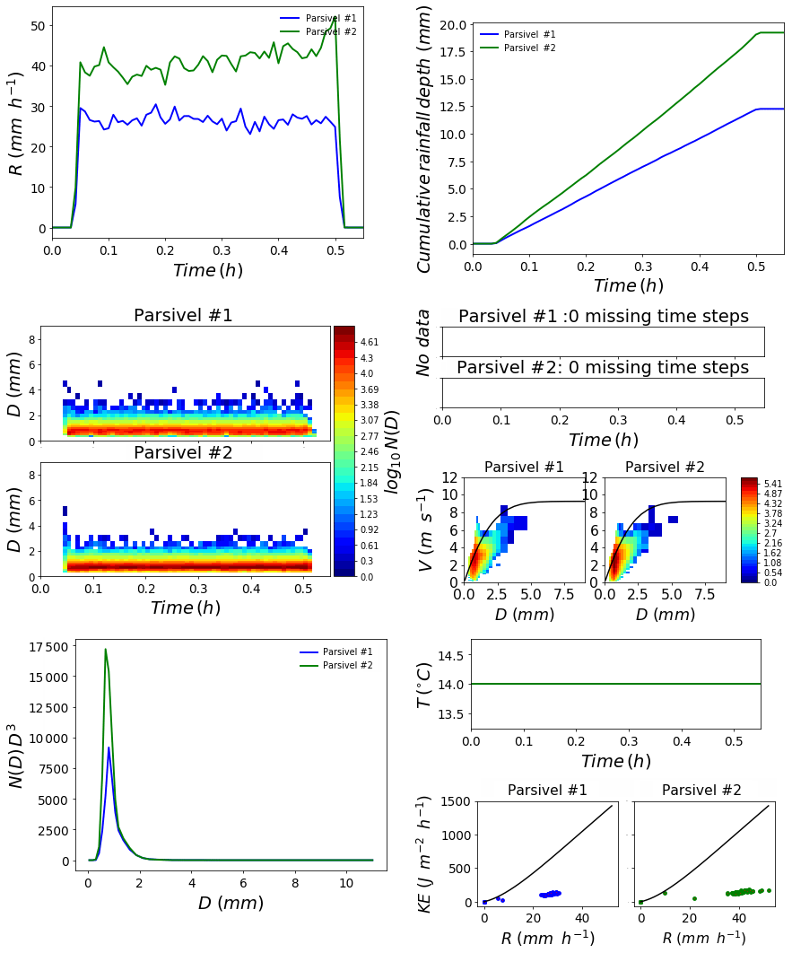
Figures 4 and 6 display quicklooks of the measurements carried out at location no. 1 with light and heavy rainfall, respectively. As an illustration, Fig. 7 displays a similar quicklook for an actual rainfall event that occurred on 10 February 2019 between 07:00:00 and 10:00:00 UTC. The disdrometers and configuration are the same as in Gires et al. (2018a). This event lasted 3 h and resulted in a total rainfall depth of roughly 6 mm. Limited rain rates lower than 10 mm h−1 were recorded during the whole event, except during roughly 10 min approximately 1 h after the beginning of the event.
The first point is the steadiness of the features of the simulated features both in terms of rain rate (upper left) or DSD (middle left), which is radically opposed to what is found in natural rainfall. It is actually a property that is wanted for a rainfall simulator. Let us simply mention that it takes a few minutes to reach a “permanent” regime in the functioning of the nozzles.
A closer look at the DSD (middle left and lower left on the quicklooks) reveals that the drops generated by the rainfall simulators are smaller than actuals ones. More precisely the DSD is much thicker and centred on smaller drops. A common indicator is the mass-weighted diameter Dm expressed in millimetres, which is equal to the ratio between the moment of the order of 4 and 3 of the DSD:
Dm was computed on average for the whole test in location no. 1 for both rainfall intensity. For light intensity it is equal to 0.99 and 0.88 mm for Pars#1 and Pars#2, respectively. Considering each time step independently it varies within the range 0.95–1.05 mm for Pars#1 and within the range 0.85–0.90 for Pars#2. With regards to the tests for heavy rainfall, on average at location no. 1 it is equal to 0.88 and 1.07 mm for Pars#1 and Pars#2, respectively. Considering each time step independently it varies within the range 0.8–0.9 mm for Pars#1 and within the range 1.0–1.2 for Pars#2. These values are significantly smaller than typical ones for actual rainfall. For instance for the event displayed in Fig. 7, we find Dm equal to 1.51 and 1.41 for Pars#1 and Pars#2, respectively, with variations between 0.8 and 3 mm during the event. Furthermore, Dm tends to increase with increasing rainfall intensities, so much greater values would be expected for rain rate generated with the simulator. It should be noted that with the simulator very few differences are found for the shape of the DSD between simulations with either light or heavy intensities.
In addition, the maps basically displaying the number of drops according to the classes of velocities and sizes (middle right in the quicklooks) show that drops tend to reach the disdrometers with lower velocities than expected. Indeed for actual rainfall, measured distribution is roughly scattered around the expected theoretical relation between the terminal fall velocity and the equivolumic diameter (solid black line). Such measured distribution is shifted toward smaller velocities. It can be noticed that this issue is more pronounced for larger drops than smaller ones, which is expected. This is due to the fact that the height of the rainfall simulator of 8 m is not sufficient to enable the drops to reach their terminal fall velocities (Beard, 1977). For instance Abd Elbasit et al. (2010) used a 12 m tower to ensure proper velocities for all sizes of drops.
As a result of both the absence of large drops and lower fall velocity, the kinetic energy of the simulated rainfall is strongly underestimated with the regards to the expected values for such rain rates. This feature is visible on the lower right panel of the quicklooks of Figs. 4 and 6. The commonly found relationship is properly retrieved for the actual rainfall (Fig. 7).
The database presented in this paper has been made available by the Hydrology, Meteorology and Complexity laboratory of École des Ponts ParisTech (HM&Co-ENPC) and the Sense-City consortium at https://doi.org/10.5281/zenodo.3686594 (Gires et al., 2019). The following citation should be used for every use of the data:
-
The following citation should be used for this paper:
Gires et al. (2020),
https://doi.org/10.5194/essd-12-835-2020. -
The following citation should be used for the database:
Gires et al. (2019),
https://doi.org/10.5281/zenodo.3686594.
This dataset is available for download free of charge. Licence terms apply. Finally it should mentioned that these disdrometers and others have been and are used in other measurement campaigns by HM&Co. Regular updates of their status along with updates of the database are to be provided through the lab's website (https://hmco.enpc.fr/, last access: 24 March 2020). The web page https://hmco.enpc.fr/portfolio-archive/taranis-observatory/ (last access: 24 March 2020) contains links to summary calendars with access to quicklooks past and ongoing measurement campaigns (daily updates).
The 30 s disdrometer data from a measurement campaign beneath a rainfall simulator are presented in this paper. Raw data as well as Python-formatted data with the associated scripts for basic manipulation are described and made available to the community for further use.
In order to discuss the features the rainfall generated by the simulator, an illustrative comparison is made with actual rainfall. It appears the properties of the rainfall generator remain steady over time, which is the desired quality. In terms of more refined properties, the drop size distribution generated is thinner than actual rainfall and centred on smaller drops. In addition the height of the simulator is not sufficient for larger drops (> 1 mm) to reach their terminal fall velocity. As a consequence the kinetic energy of the simulated rainfall is smaller than in actual rainfall for a similar rain rate. In order to interpret the reproducible experiments that can be carried out with the help of such a rainfall simulator, these features should be accounted for and analysed more in depth. Their relative importance will depend on the specific studied issue.
The research grants obtained respectively by DS and AR permitted the acquisition of the scientific equipment and realization of experimental facilities. IT and AG designed the study. AG and PB carried out the measurement campaign. AG wrote the paper. The joint discussion and analysis by all the authors of the obtained data and results shaped the paper into its actual form.
The authors declare that they have no conflict of interest.
The authors greatly acknowledge partial financial support from the Chair of Hydrology for Resilient Cities (endowed by Veolia) of the École des Ponts ParisTech, and the Île-de-France region RadX@IdF Project. We also want to thank ANR, the French Funding Agency, for supporting Sense City Equipex.
This study received financial support from the Chair of Hydrology for Resilient Cities (endowed by Veolia) of the École des Ponts ParisTech, and the Île-de-France region RadX@IdF Project.
This paper was edited by Scott Stevens and reviewed by two anonymous referees.
Abd Elbasit, M. A. M., Yasuda, H., Salmi, A., and Anyoji, H.: Characterization of rainfall generated by dripper-type rainfall simulator using piezoelectric transducers and its impact on splash soil erosion, Earth Surf. Proc. Land., 35, 466–475, https://doi.org/10.1002/esp.1935, 2010. a, b
Angulo-Martínez, M. and Barros, A.: Measurement uncertainty in rainfall kinetic energy and intensity relationships for soil erosion studies: An evaluation using PARSIVEL disdrometers in the Southern Appalachian Mountains, Geomorphology, 228, 28–40, https://doi.org/10.1016/j.geomorph.2014.07.036, 2015. a, b
Auerswald, K., Kainz, M., Schröder, D., and Martin, W.: Comparison of German and Swiss Rainfall Simulators – Experimental Setup, Z. Pflanz. Bodenkunde, 155, 1–5, https://doi.org/10.1002/jpln.19921550102, 1992. a
Battaglia, A., Rustemeier, E., Tokay, A., Blahak, U., and Simmer, C.: PARSIVEL Snow Observations: A Critical Assessment, J. Atmos. Ocean. Tech., 27, 333–344, https://doi.org/10.1175/2009JTECHA1332.1, 2010. a
Beard, K. V.: Terminal velocity adjustment for cloud and precipitation aloft, J. Atmos. Sci, 34, 1293–1298, 1977. a
Gires, A., Tchiguirinskaia, I., and Schertzer, D.: Multifractal comparison of the outputs of two optical disdrometers, Hydrol. Sci. J., 61, 1641–1651, https://doi.org/10.1080/02626667.2015.1055270, 2015. a
Gires, A., Tchiguirinskaia, I., and Schertzer, D.: Two months of disdrometer data in the Paris area, Earth Syst. Sci. Data, 10, 941–950, https://doi.org/10.5194/essd-10-941-2018, 2018a. a, b, c, d, e, f, g, h, i
Gires, A., Tchiguirinskaia, I., and Schertzer, D.: Pseudo-radar algorithms with two extremely wet months of disdrometer data in the Paris area, Atmos. Res., 203, 216–230, https://doi.org/10.1016/j.atmosres.2017.12.011, 2018b. a
Gires, A., Bruley, P., Ruas, A., Schertzer, D., and Tchiguirinskaia, I.: Data for “Disdrometer measurements under Sense-City rainfall simulator”, Zenodo, https://doi.org/10.5281/zenodo.3686594, 2019. a, b, c, d
Gires, A., Bruley, P., Ruas, A., Schertzer, D., and Tchiguirinskaia, I.: Disdrometer measurements under Sense-City rainfall simulator, Earth Syst. Sci. Data, 12, 835–845, https://doi.org/10.5194/essd-12-835-2020, 2020. a
Hall, M. J.: A Critique of Methods of Simulating Rainfall, Water Resour. Res., 6, 1104–1114, https://doi.org/10.1029/WR006i004p01104, 1970. a
Humphry, J. B., Daniel, T. C., Edwards, D. R., and Sharpley, A. N.: A Portable Rainfall Simulator for Plot–Scale Runoff Studies, Appl. Eng. Agr., 18, 199–204, https://doi.org/10.13031/2013.7789, 2002. a
Iserloh, T., Fister, W., Seeger, M., Willger, H., and Ries, J.: A small portable rainfall simulator for reproducible experiments on soil erosion, Soil Till. Res., 124, 131–137, https://doi.org/10.1016/j.still.2012.05.016, 2012. a
Jaffrain, J. and Berne, A.: Quantification of the Small-Scale Spatial Structure of the Raindrop Size Distribution from a Network of Disdrometers, J. Appl. Meteorol. Clim., 51, 941–953, https://doi.org/10.1175/JAMC-D-11-0136.1, 2012. a
Lhermitte, R. M.: Cloud and precipitation remote sensing at 94 GHz, IEEE T. Geosci. Remote, 26, 207–216, 1988. a
Loffler-Mang, M. and Joss, J.: An Optical Disdrometer for Measuring Size and Velocity of Hydrometeors, J. Atmos. Ocean. Tech., 17, 130–139, https://doi.org/10.1175/1520-0426(2000)017<0130:AODFMS>2.0.CO;2, 2000. a
Meshesha, D. T., Tsunekawa, A., Tsubo, M., Haregeweyn, N., and Tegegne, F.: Evaluation of kinetic energy and erosivity potential of simulated rainfall using Laser Precipitation Monitor, CATENA, 137, 237–243, https://doi.org/10.1016/j.catena.2015.09.017, 2016. a
Olayemi, F. and Yadav, R.: Rainfall simulator for tillage research in the tropics, Soil Till. Res., 3, 397–405, https://doi.org/10.1016/0167-1987(83)90041-7, 1983. a
OTT: Operating instructions, Present Weather Sensor OTT Parsivel2, 2014. a, b
Paige, G., Stone, J., Smith, J., and Kennedy, J.: The Walnut Gulch Rainfall Simulator: A computer-controlled variable intensity rainfall simulator, ASAE Appl. Eng. Agric., 20, 25–31, https://doi.org/10.13031/2013.15691, 2004. a
Parsons, A. J., Stromberg, S. G. L., and Greener, M.: Sediment-transport competence of rain-impacted interrill overland flow, Earth Surf. Proc. Land., 23, 365–375, https://doi.org/10.1002/(SICI)1096-9837(199804)23:4<365::AID-ESP851>3.0.CO;2-6, 1998. a
Salles, C. and Poesen, J.: Rain properties controlling soil splash detachment, Hydrol. Proc., 14, 271–282, https://doi.org/10.1002/(SICI)1099-1085(20000215)14:2<271::AID-HYP925>3.0.CO;2-J, 2000. a
Thurai, M. and Bringi, V. N.: Drop Axis Ratios from a 2D Video Disdrometer, J. Atmos. Ocean. Technol., 22, 966–978, https://doi.org/10.1175/JTECH1767.1, 2005. a