the Creative Commons Attribution 4.0 License.
the Creative Commons Attribution 4.0 License.
 | 09 Dec 2020
A global long-term (1981–2000) land surface temperature product for NOAA AVHRR
Ji Zhou
Frank-Michael Göttsche
Shunlin Liang
Shaofei Wang
Mingsong Li
Land surface temperature (LST) plays an important role in the research of climate change and various land surface processes. Before 2000, global LST products with relatively high temporal and spatial resolutions are scarce, despite a variety of operational satellite LST products. In this study, a global historical LST product is generated from NOAA advanced very-high-resolution radiometer (AVHRR) data (1981–2000), which includes three data layers: (1) instantaneous LST, a product generated by integrating several split-window algorithms with a random forest (RF-SWA); (2) orbital-drift-corrected (ODC) LST, a drift-corrected version of RF-SWA LST; and (3) monthly averages of ODC LST. For an assumed maximum uncertainty in emissivity and column water vapor content of 0.04 and 1.0 g cm−2, respectively, evaluated against the simulation dataset, the RF-SWA method has a mean bias error (MBE) of less than 0.10 K and a standard deviation (SD) of 1.10 K. To compensate for the influence of orbital drift on LST, the retrieved RF-SWA LST was normalized with an improved ODC method. The RF-SWA LST were validated with in situ LST from Surface Radiation Budget (SURFRAD) sites and water temperatures obtained from the National Data Buoy Center (NDBC). Against the in situ LST, the RF-SWA LST has a MBE of 0.03 K with a range of −1.59–2.71 K, and SD is 1.18 K with a range of 0.84–2.76 K. Since water temperature only changes slowly, the validation of ODC LST was limited to SURFRAD sites, for which the MBE is 0.54 K with a range of −1.05 to 3.01 K and SD is 3.57 K with a range of 2.34 to 3.69 K, indicating good product accuracy. As global historical datasets, the new AVHRR LST products are useful for filling the gaps in long-term LST data. Furthermore, the new LST products can be used as input to related land surface models and environmental applications. Furthermore, in support of the scientific research community, the datasets are freely available at https://doi.org/10.5281/zenodo.3934354 for RF-SWA LST (Ma et al., 2020a), https://doi.org/10.5281/zenodo.3936627 for ODC LST (Ma et al., 2020c), and https://doi.org/10.5281/zenodo.3936641 for monthly averaged LST (Ma et al., 2020b).
- Article
(5890 KB) - Full-text XML
- BibTeX
- EndNote


Land surface temperature (LST) is an important parameter for energy exchange between Earth's surface and the atmosphere and thus an important indicator for global climate change. Therefore, LST has been widely used in research and applications of land surface processes and models, e.g., climate and meteorology, hydrology, and disaster monitoring (Anderson et al., 2011; Jin and Dickinson, 2002; Van Der Werf et al., 2017). Compared to traditional ground observations, retrieving LST from remote sensing is an effective way of taking advantage of the spatiotemporal coverage offered by satellites. Since the 1970s, the accurate retrieval of LST from satellite has been an active area of research in quantitative remote sensing. The main sources for retrieving LST from satellite data are thermal-infrared (TIR) remote sensing and passive microwave (MW) remote sensing (Holmes et al., 2009; Li et al., 2013a), which both are effective means for obtaining the radiance emitted by Earth's surface. Although MW remote sensing is less affected by cloud and fog, when compared to TIR remote sensing, it is limited by factors such as coarser spatial resolution, higher thermal sampling depth, and higher uncertainty in emissivity, which results in a lower retrieval accuracy (Zhou et al., 2017). Therefore, retrieving LST from TIR remote sensing is still the dominant approach, since it offers a better physical definition and higher retrieval accuracy. LST retrieval from satellite TIR remote sensing is based on the simplification of the radiative transfer model. A variety of algorithms have been proposed for retrieving LST from TIR data, e.g., split-window algorithms (SWA), mono-window algorithms or single-channel algorithms, and temperature-emissivity separation algorithms (TESs) (Gillespie et al., 1998; Li et al., 2013a; Wan and Dozier, 1996). Selecting a suitable algorithm for retrieving LST depends on the sensor's number of TIR channels and their spectral specifications, as well as the available auxiliary input data.
The SWA is a good choice for retrieving LST from sensors with two or more TIR channels centered at 11 and 12 µm, e.g., Terra/Aqua MODIS, NOAA advanced very-high-resolution radiometer (AVHRR), ENVISAT AATSR, and Sentinel-3 SLSTR. Based on the idea that the atmospheric absorption in the thermal band can be related to the brightness temperature (BT) difference between two adjacent channels, McMillin (1975) initially proposed the SWA for retrieving sea surface temperature (SST) from NOAA/AVHRR. SWAs for retrieving SST from various sensors were developed, which were based on different assumptions (Llewellyn-Jones et al., 1984; Niclòs et al., 2007). Inspired by the success of the SST algorithm, the first SWA for retrieving LST was proposed by Price (1984). However, in contrast to nearly homogeneous and isothermal water bodies, LST is affected by multiple additional factors, e.g., land cover type (LCT), material-dependent emissivity, terrain, and viewing geometry. Therefore, one or more terms were added to the basic SWA to describe these effects, e.g., land surface emissivity (Wan, 2014), vegetation cover fraction (Prata, 2002), view zenith angle (Becker and Li, 1990a), and water vapor (Sobrino et al., 1991). Nevertheless, there are still limitations in LST retrieval with SWAs (Li et al., 2013a), e.g., the requirement for a priori knowledge of emissivity and a dependence of LST retrieval accuracy on SW coefficients, which in turn depend on observation and atmospheric conditions. Furthermore, due to the variation of land surface and atmospheric conditions, no single SWA performs the best under all conditions (Yang et al., 2020; Yu et al., 2009; Zhou et al., 2019b).
Currently, several LST products derived from satellite TIR remote sensing are available. Global LST products for Terra/Aqua MODIS are available dating back to 2000, e.g., MOD11/MYD11 (Wan, 2008, 2014; Wan et al., 2002) and MOD21/MYD21 (Hulley and Hook, 2011). Similarly, a JPSS-VIIRS LST product is available dating back to 2012 (Guillevic et al., 2014) and China FengYun-VIRR LST is available dating back to 2009 (Dong et al., 2012). The aforementioned sensors observe Earth's surface twice per day with a spatial resolution of ∼ 1 km at nadir. For the user's convenience, some LST products are processed into different temporal and spatial resolutions, e.g., daily, monthly, 1 km × 1 km, . The operational LST product retrieved from the (A)ATSR series between 1995 and 2012 is a typical SWA LST product (Prata, 2002). AATSR's nadir spatial resolution onboard ENVISAT was approximately 1 km, and its temporal resolution was 3 d. Since 2016, its successor, SLSTR onboard Sentinel-3 A and B, provides daily temporal resolution and a consistent spatial resolution (Ghent et al., 2017). Global LSTs retrieved from satellite TIR also include Landsat LST (Parastatidis et al., 2017) and ASTER LST (Hulley and Hook, 2011), which have significantly higher spatial resolutions (e.g., about 100 m) but considerably lower temporal resolutions (e.g., every 16 d). LST products from geostationary satellites are generated at lower spatial resolution (3–5 km) but considerably higher temporal resolution (10–60 min), e.g., GOES-ABI LST for the Americas and Africa (Yu et al., 2009); MSG-MVIRI/SEVIRI LST for Europe, Africa, and the Atlantic Ocean (Duguay-Tetzlaff et al., 2015; Trigo et al., 2008); and FY-SVISSR/AGRI LST and Himawari-AHI LST for the Asia-Pacific region (Choi and Suh, 2018; Jiang and Liu, 2014). Dech et al. (1998) and Pinheiro et al. (2006) provide African and European LST for NOAA-14 AVHRR; Zhou et al. (2019a) provide an all-weather LST product retrieved from combined TIR and MW data over the Tibetan plateau from 2003 to 2018. There are also a few LST products from MW (e.g., for SSM/I and AMSR-E) (Aires et al., 2001; Jiménez et al., 2017) and LST for land surface models (e.g., ECMWF and GLDAS) (Fang et al., 2009; Viterbo and Beljaars, 1995); however, these LST products have lower spatial resolutions and slightly different meanings than TIR LST. In summary, from 1991 onwards, many global and regional satellite LST products are available, but higher spatiotemporal resolutions (e.g., 1 km – daily) are only available after 2000. At the same time, many climate applications urgently need higher spatiotemporal resolution LST products for the time before 2000. It has been reported that 1983–2012 was the warmest 30 years for nearly 1400 years (IPCC, 2014). The warm climate change trend has also caused changes in many land surface processes, e.g., most glaciers on the Tibetan Plateau are in retreat and the areas covered by them are getting smaller and smaller (Yao et al., 2012). The LST around glaciers is a highly useful indicator of this phenomenon and allows for predicting trends in glacier status (Steiner et al., 2008). Similar demands for LST data also exist in global drought monitoring (Sánchez et al., 2018), studies of species distribution (Lembrechts et al., 2019), and land surface modeling (Bechtel, 2012; Ghent et al., 2017; Reichle et al., 2010). Therefore, it is meaningful to extend the global LST time series with a relatively high spatiotemporal resolution (i.e., 5 km and daily) to the historical NOAA AVHRR data before 2000.
A major factor limiting applications of AVHRR LST is orbital drift, which over the lifespan of the NOAA satellites leads to shifts to later overpass times and, therefore, affects temporal comparability. Two main approaches were developed to remove the effect of orbital drift. On the one hand, based on the regular diurnal temperature variation typically observed under clear sky, several researchers corrected orbital drift by fitting a diurnal temperature cycle (DTC) model to reanalysis or geostationary datasets (Jin and Treadon, 2003; Parton and Logan, 1981) and then normalizing LST to a given time. On the other hand, a relationship between LST anomaly and solar zenith angle was used for correcting LST to a given solar zenith angle (Gleason et al., 2002; Gutman, 1999; Julien and Sobrino, 2012). Various applications made use of the two types of orbital drift correction methods for AVHRR LST, but a general method for global application is still missing; i.e., the former method suffers from the low spatial resolution of its input datasets, while the latter leads to inconsistent times. Liu et al. (2019a) proposed another method for correcting AHVRR LST orbital drift, which fits a DTC model to component temperatures of neighborhood pixels and was reported to achieve good accuracy.
As a part of the Global LAnd Surface Satellite (GLASS) product suite (Liang et al., 2020), the objective of this study is to develop a long-term global LST product (1981–2000) from historical NOAA AVHRR datasets. Section 2 describes the simulation datasets used for developing consistent SWAs, the input datasets for LST product generation, and the in situ datasets for validating the retrieved LST. In Sect. 3, a practical approach for generating a single optimized LST product is proposed, which integrates several well-established SWAs through the random forest, which is termed RF-SWA. Finally, the retrieved RF-SWA LST is normalized with an improved orbital drift correction method. Furthermore, emissivity estimation for bare soil is improved by using ASTER Global Emissivity Dataset (GED) and yields more accurate estimates of land surface emissivity in Sect. 3.3. Section 4 describes the results and provides implementation details of the LST retrieval method, LST validation, and gives an example of the LST product. Data availability is given in Sect. 5. Conclusions and outlooks are provided in Sect. 6.
2.1 Satellite remote sensing datasets
2.1.1 AVHRR datasets
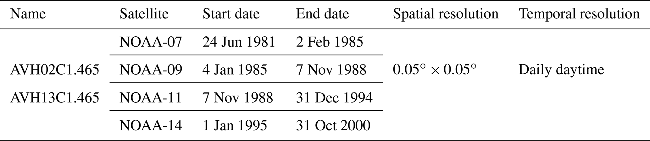
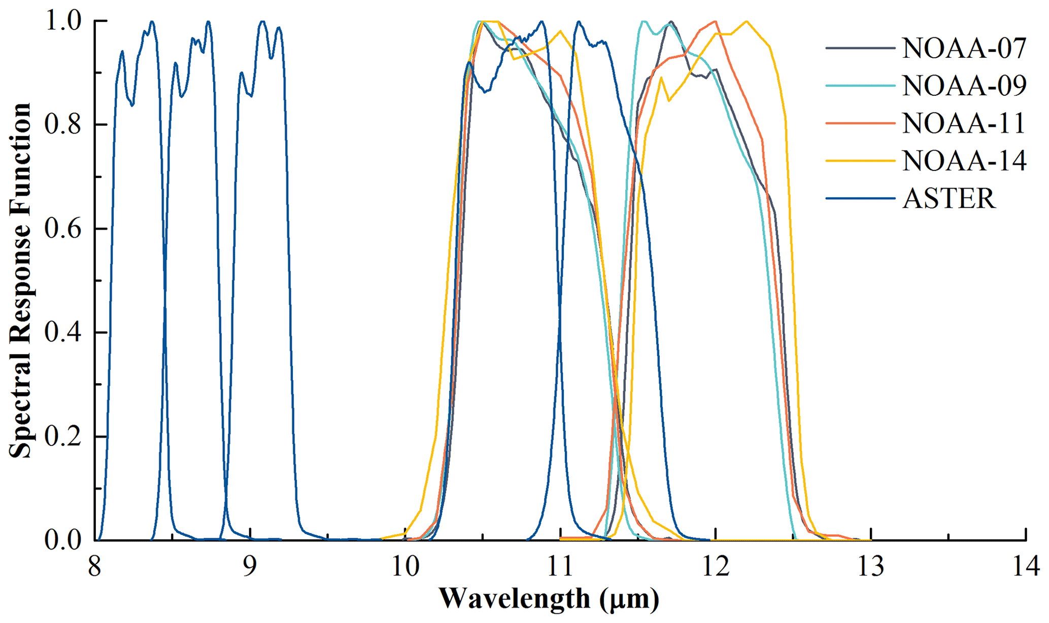
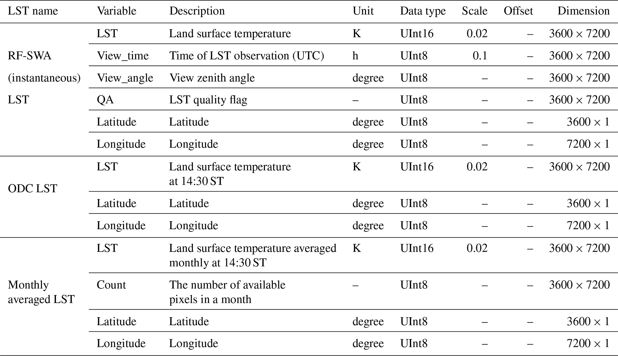
The advanced very-high-resolution radiometer (AVHRR) is a sensor onboard NOAA polar-orbiting satellite series. The orbital period is 101.4 min and designed over-pass time at the Equator is between 13:30 and 14:30 ST (solar time) depending on the satellite. The second AVHRR version (AVHRR/2) has five spectral channels, including a visible band (0.55–0.68 µm), a near-infrared band (0.75–1.1 µm), a middle-infrared band (3.55–3.93 µm), and two thermal bands (10.5–11.3 and 11.5–12.5 µm). Figure 1 shows the spectral responses of the two AVHRR thermal channels of NOAA-07/09/11/14. Nadir spatial resolution of the TIR channels is 1.1 km × 1.1 km, and scan angles range between −55 and 55∘. AVHRR covers the Earth's surface twice daily and has been widely used to generate various local or global land and sea surface parameters, e.g., the normalized difference vegetation index (NDVI) and SST (Casey et al., 2010). In this study, the AVHRR datasets from Long-Term Dataset Records (Pedelty et al., 2007) (LTDR, https://ltdr.modaps.eosdis.nasa.gov/, last access: 2 December 2020) are used, including AVH02C1 and AVH13C1, for which spatial resolution has been processed to 0.05∘ × 0.05∘ (Table 1). Those two datasets include the top-of-atmosphere BT of the TIR channels, NDVI, view zenith angle (VZA), view time, and quality control (QC) flags, which provide a reference for distinguishing pure and cloudy pixels.
2.1.2 ASTER Global Emissivity Dataset (GED)
ASTER, onboard the Terra satellite, and has five TIR channels (Fig. 1). The ASTER GED used in this study was generated from clear sky ASTER TIR data between 2000 and 2008 with the TES algorithm and the water vapor scaling atmosphere correction method (Hulley et al., 2015). The products are output at 3′′ (∼ 100 m) and 30′′ (∼ 1 km) spatial resolution on tiles. Channel temporal mean emissivity, LST, and NDVI, as well as their standard deviation, global digital elevation model (DEM), and land–sea mask, are part of the GED. In this study, the ASTER GEDv3 with a 1 km spatial resolution was used to determine the global background emissivity of bare land.
2.2 Atmospheric profiles and forward simulation datasets
Global forward simulation datasets with good representativeness are necessary for developing and evaluating LST retrieval algorithms. This requires a reliable atmospheric profile dataset as input. In this study, the well-established SeeBor V5.0 (Borbas et al., 2005) and TIGR2000 V1.2 .(Chedin et al., 1985) atmospheric profiles were used to construct the forward simulation datasets. Zhou et al. (2019b) derived a global atmospheric profile dataset (GAPD) by screening the SeeBor V5.0 atmospheric profiles and removing cloud-contaminated and redundant profiles. The GAPD dataset has been used for developing the LST retrieval algorithm for NOAA-20/VIIRS and Sentinel-3/SLSTR (Liu et al., 2019b; Yang et al., 2020): it contains 549 global profiles with a column water vapor content (CWVC) range of 0.014–7.939 g cm−2 and near-surface air temperature (NSAT) range of 224.25–309.05 K. Here, the GAPD was used to generate a training dataset (TRA-G): globally representative observation conditions were simulated by varying the viewing geometry and land surface characteristics over a realistic range for a limited profile dataset (Zhou et al., 2019b), i.e., for each profile 10 surface temperatures (Ts), 15 view zenith angles (VZA), and 48 land surface emissivities (LSEs, ε) were set. Specifically, Ts was set relative to NSAT with the difference (Ts-NSAT) covering the range of −16 to +20 K at an interval of 4 K. VZA was set to values from 0 to 70∘ at an interval of 5∘. Emissivity was obtained from Johns Hopkins University (JHU) spectral emissivity library by convolving the emissivity spectra with the spectral response functions of NOAA-07, 09, 11, and 14 AVHRR (Fig. 1). The corresponding emissivity ranges are provided in Table 2. For the remaining 4761 SeeBor clear-sky profiles (ATP-S) and 506 TIGR clear-sky profiles (ATP-T), the corresponding simulations were performed and used as evaluation datasets VAL-S and VAL-T, respectively. In contrast to GAPD, for each profile in ATP-S (ATP-T), we randomly set 10 (10) VZAs between 0 and 70∘. The corresponding LSE has been assigned according to the LCT over which a profile is located (Snyder et al., 1998) and Ts for VAL-S and VAL-T was set to the corresponding NSAT. Table 3 summarizes the three profile datasets and the corresponding simulation datasets. More details can be found in Zhou et al. (2019b) and Yang et al. (2020).
Table 2Global LSE ranges determined from JHU spectral emissivity library for AVHRR channel centered at 11 and 12 µm.
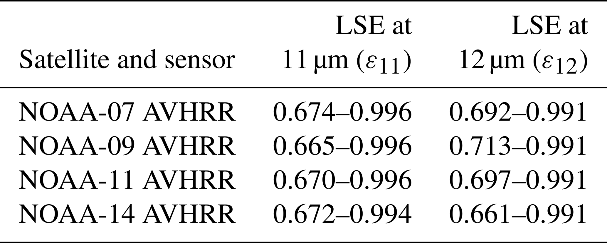
Table 3Atmospheric profile datasets and corresponding simulation datasets.

2.3 Ancillary data used for LST retrieval
Four ancillary datasets were used for LST retrieval: NSAT, CWVC, LCT, and soil type. The MERRA-2 reanalysis dataset (M2T1NXSLV) provides NSAT and CWVC (variables in datasets: T2M and TQV, respectively) with spatial resolution and hourly temporal resolution; nearest-neighbor sampling was used to match up with AVHRR pixel and overpass time. AVHRR LCTs were obtained from the University of Maryland (UMD) dataset (Defries and Hansen, 2010), which provides 14 LCTs (0: Water; 1: Evergreen Needleleaf Forest; 2: Evergreen Broadleaf Forest; 3: Deciduous Needleleaf Forest; 4: Deciduous Broadleaf Forest; 5: Mixed Forest; 6: Woodland; 7: Wooded Grassland; 8: Closed Shrubland; 9: Open Shrubland; 10: Grassland; 11: Cropland; 12: Bare Ground; 13: Urban and Built). The spatial resolution of the UMD LCT dataset is 1 km × 1 km. To adapt its resolution of AVHRR, the dominant LCT within each 0.05∘ grid was used as the LCT for AVHRR. The soil type dataset employed for estimating AVHRR LSE is provided by the United States Department of Agriculture, which is mainly based on the world soil map of FAO-UNESCO. Its spatial resolution is 2′ (∼ 0.03∘), and the soil type of each AVHRR pixel was also set to the dominant type.
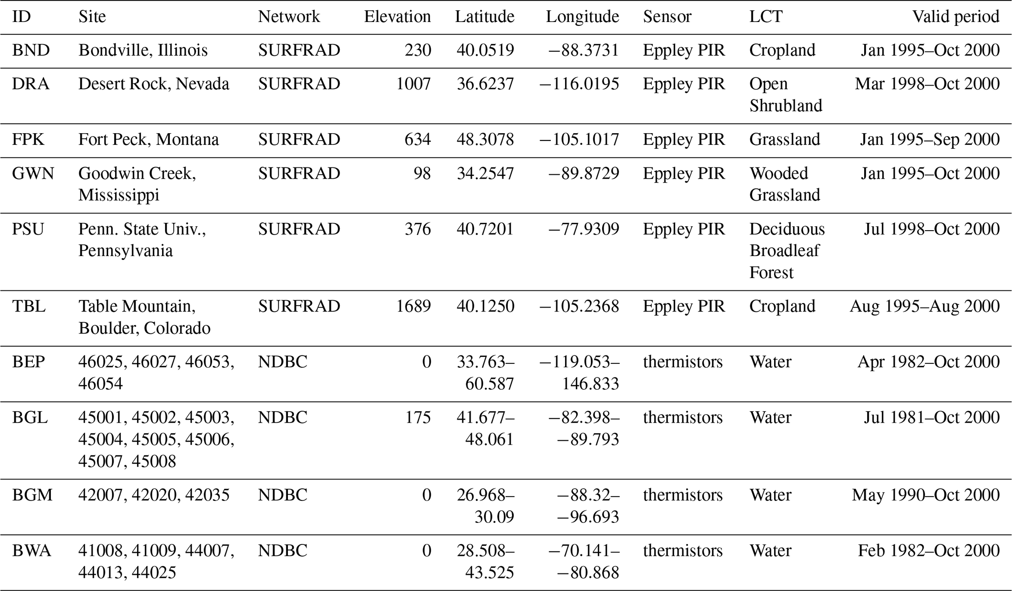
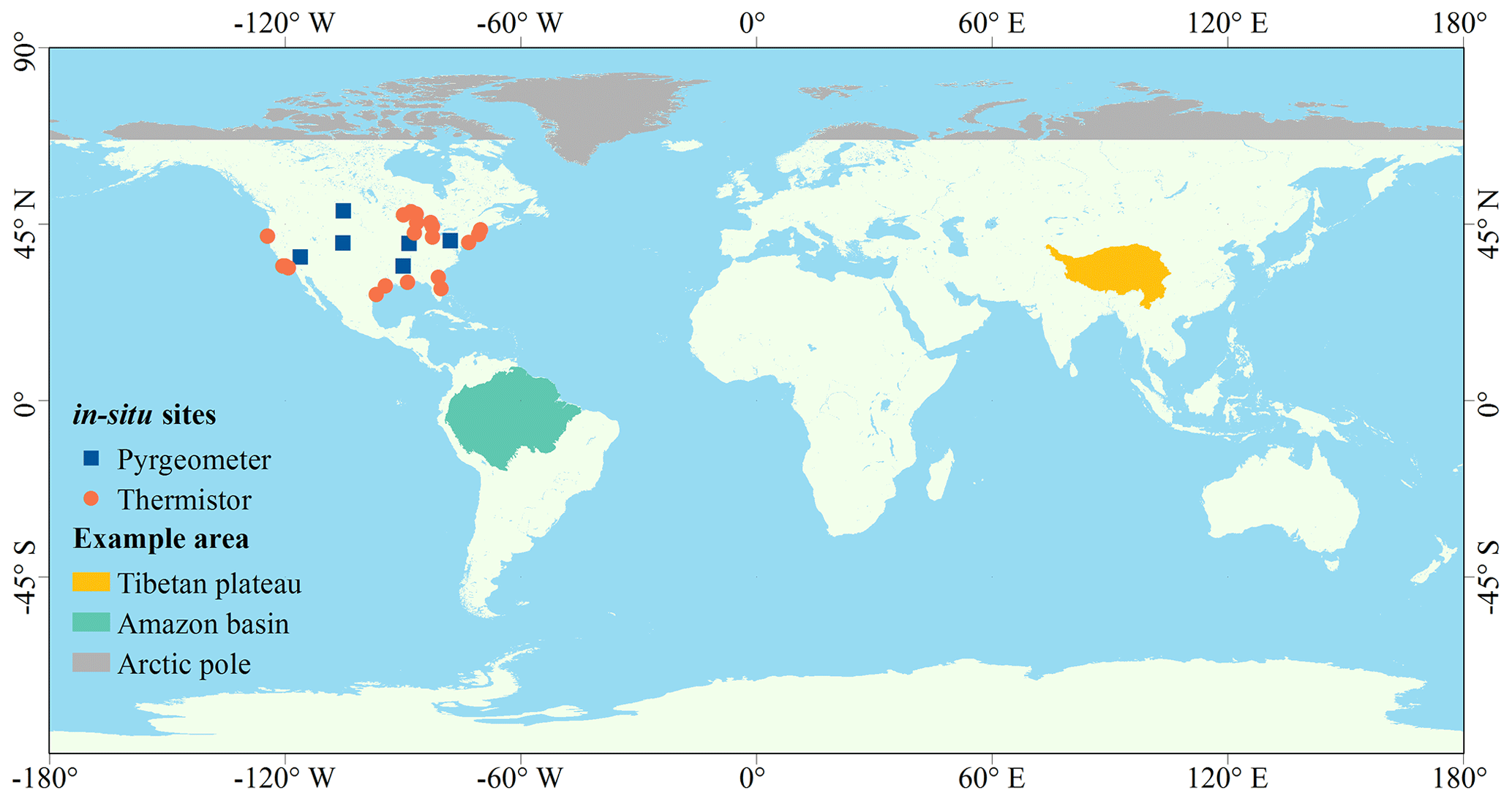
Figure 2Locations of SURFRAD sites and NDBC buoys and the three sample areas. Blue squares indicate pyrgeometers; red circles indicate contact thermistors.
2.4 In situ datasets
In situ measurements from the Surface Radiation Budget (SURFRAD) network and the National Data Buoy Center (NDBC) were used to validate the retrieved AVHRR LST. The details and geographical distribution of the selected in situ sites are provided in Table 4 and Fig. 2. SURFRAD was established in 1993 and focuses on validating Earth's radiation budget. Quality control is an integral part of the design and operation of the SURFRAD network, which results in datasets of high-quality and well-defined measurement uncertainties (https://www.esrl.noaa.gov/gmd/grad/surfrad/, last access: 2 December 2020). Therefore, SURFRAD data have been widely used for validating satellite-retrieved LST products (Guillevic et al., 2014; Liu et al., 2019b; Martin et al., 2019; Wang and Liang, 2009) and other fields. Six sites providing in situ data between 1995 and 2000 were selected. At these sites, upwelling and downwelling longwave radiances are measured with highly accurate Eppley Precision Infrared Radiometers (PIR; wavelength: 4–50 µm) at an observation interval of 3 min. The PIRs were set up ∼ 10 m above the ground, giving them a field of view (FOV) covering approximately 70×70 m2 (Guillevic et al., 2014). Historical data from the NDBC (https://www.ndbc.noaa.gov/historical_data.shtml, last access: 2 December 2020) provide hourly samples of bulk water temperature measured with electronic thermistors, which are highly accurate and quality-controlled by NDBC (https://www.ndbc.noaa.gov/qc.shtml, last access: 2 December 2020). Considering the thermal homogeneity of the water surface, buoy temperatures are usually representative of the satellite pixel scale, even if it covers large areas. To avoid mixed land–water pixels, only buoys at least 20 km from the coastline were selected.
Table 5Initial candidate split-window algorithms (SWAs).
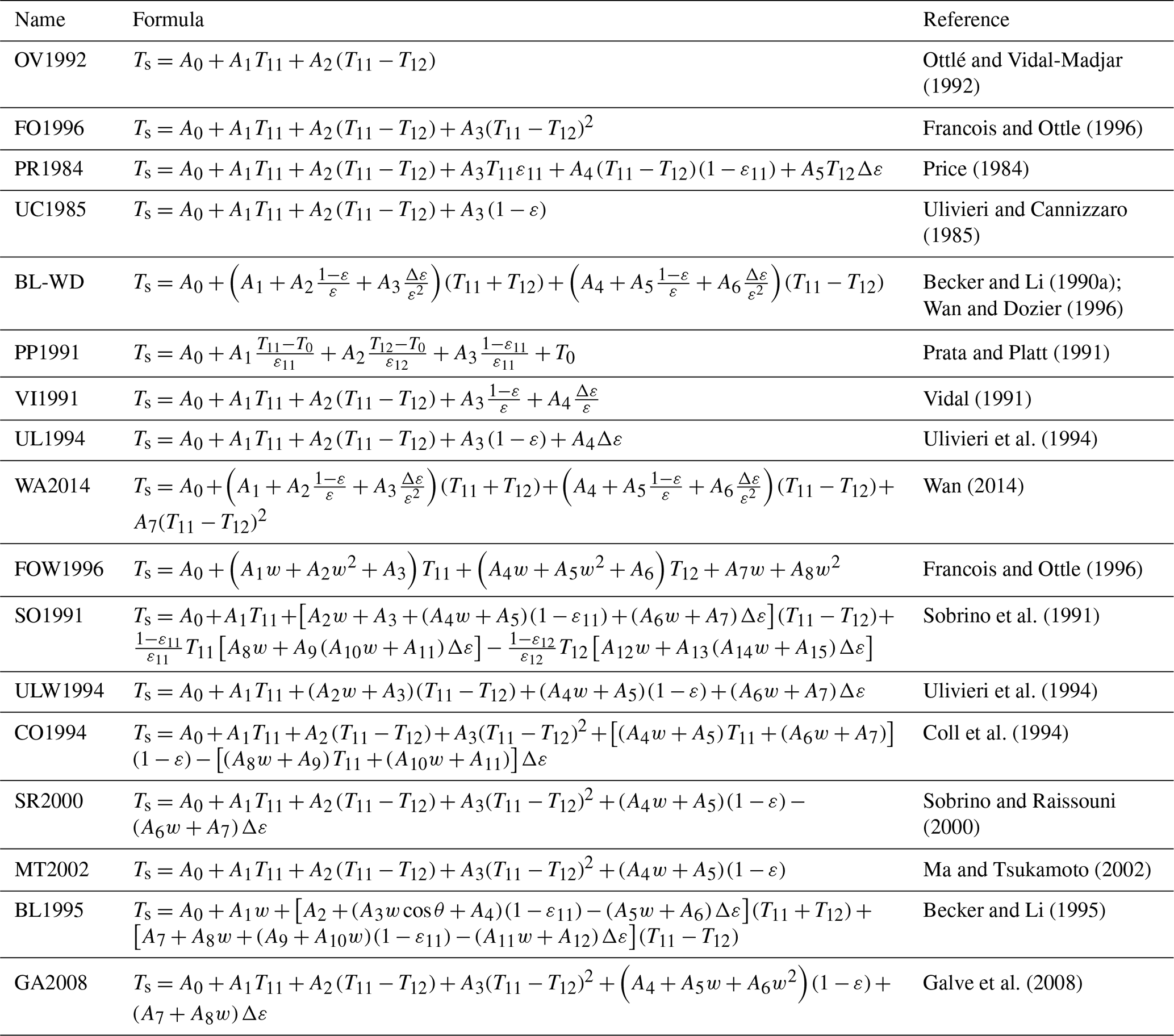
Note that subscripts 11 and 12 denote channels centered at approximately 11 and 12 µm, respectively, while T11 and T12 and ε11 and ε12 are their associated BTs and LSEs; , Δε=(ε11-ε12), Ai are coefficients, T0 in PP1991 is 273.15 K, w is CWVC, and θ is VZA.
Using an LST retrieval algorithm from TIR remote sensing, especially with SWAs, is a well-established and validated method. However, no single algorithm performs best under all conditions, even if it generally achieves good accuracy (Yu et al., 2009). This suggests that a more stable and robust LST retrieval algorithm may be obtained by integrating various individual LST retrieval algorithms. In this study, the random forest (RF) ensemble method (Breiman, 2001) was utilized for integrating multi-LSTs (mLSTs) obtained with several SWAs into a global AVHRR LST product. First, widely used candidate SWAs were trained and evaluated; these SWAs have been studied in previous work (Yang et al., 2020; Zhou et al., 2019b) and are shown in Table 5 for readers' convenience. Second, estimates of land surface emissivity were improved by combining the NDVI threshold method and ASTER GED. Third, the LSTs from the trained candidate SWAs were integrated with the RF method: thus, the approach is termed RF-SWA. Then, the instantaneous RF-SWA LST was normalized to 14:30 ST (solar time) using an improved orbital drift correction (ODC) method and the RF-SWA LST and ODC LST products were validated against in situ LST. Finally, for the user's convenience, a monthly averaged LST was also generated from the ODC LST with a sample averaging procedure.
3.1 Refining the candidate algorithms
Forward radiative transfer simulations with PMODTRAN (Berk et al., 2005; Huang et al., 2016) were performed on a high-performance computing platform (2Intel @Xeon E5-2650 2.00 GHz (8Cores), 64 GB 1600 MHz) for the datasets GAPD, ATP-S, and ATP-T described in Sect. 2.2; the corresponding simulated datasets were labeled TRA-G, VAL-S, and VAL-T. Each forward simulation yields channel-specific top-of-atmosphere radiances and BTs dependent on NSAT, CWVC, and VZA. To simulate BTs measured by satellites more realistically, Gaussian-distributed noise with a noise equivalent differential temperature (NEΔT) of 0.12 K, which is one of the design goals for the AVHRR TIR channels, was added to the simulated BTs. More details about the simulations are provided in Zhou et al. (2019b).
Multiple regression was performed on the simulated training datasets, TRA-G, to determine the coefficients of the candidate SWAs in Table 5. The TRA-G dataset was divided into 480 groups based on NSAT, CWVC, VZA, and Ts-NSAT as follows: (i) the atmospheres were divided into Cold-ATM and Warm-ATM with a NSAT threshold of 280 K, and (ii) the data were divided into CWVC classes with an interval of 0.5 g cm−2. This resulted in 3 subgroups of Cold-ATM and 13 subgroups of Warm-ATM. (iii) The VZAs were divided into intervals of 5∘. (iv) Based on Ts-NSAT, the data were divided into two subgroups, i.e., [−16,4] K and [−4, 20] K, approximately representing daytime and nighttime cases, respectively. Based on regression against these training datasets, look-up tables (LUTs) with coefficients for each candidate SWA were established. The candidate algorithms were then analyzed with respect to the standard error of the estimate (SEE) and coefficient of determination (R2), and a sensitivity analysis was performed for the main input parameters, e.g., LSE and CWVC, to test the stability and accuracy of the trained SWAs. Being consistent with the uncertainty level in Zhou et al. (2019b), the various uncertainty sources were grouped into two levels: (i) L1, i.e., , , and |δCWVC g cm−2, and (ii) L2, i.e., 0.04, 0.04, and |δCWVC g cm−2. These uncertainties will be added to ε11, ε12, and CWVC as random noises. Datasets without added uncertainty were labeled L0. All trained candidate algorithms were evaluated against the simulation datasets VAL-S and VAL-T.
3.2 Multi-LST ensemble
Based on the training and evaluation results (see Sect. 4.1), a multi-LST ensemble method is proposed, which hopefully achieves a more stable retrieval by integrating the most robust and stable SWAs. The method used to integrate the selected SWAs is the Random Forest (RF) method proposed by Breiman (2001). Compared to detailed analytic expressions for explaining complicated nonlinear relationships, the RF method has several advantages, including the ability to process large databases with high efficiency, unbiased estimation, and especially minimizing the risk of overfitting (Hutengs and Vohland, 2016). Therefore, the RF method has been widely used in remote sensing applications, e.g., land cover classification (Rodriguez-Galiano et al., 2012), land surface parameter downscaling (Zhao et al., 2018), and estimating vegetation cover parameters (Mutanga et al., 2012).
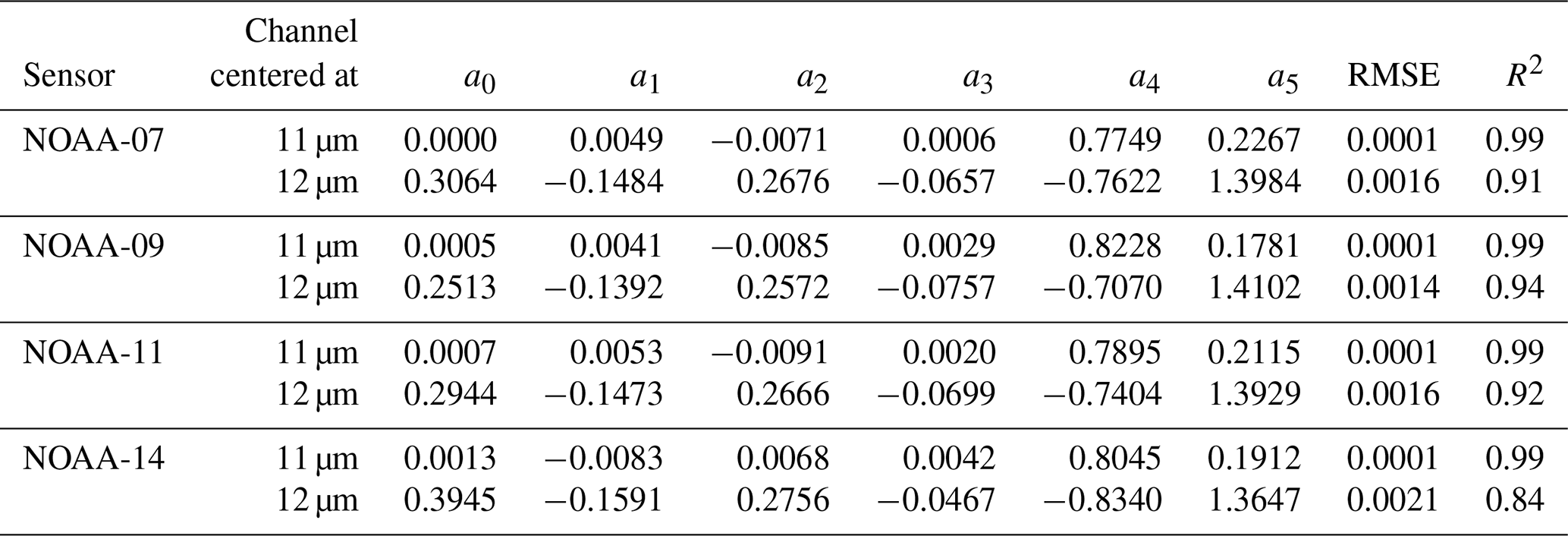
Table 6Coefficients for converting bare soil emissivity from ASTER to AVHRR (see Sect. 3.3).
The RF method utilizes an ensemble of many decision trees. In the implementation of the RF ensemble method, a random vector Θk is selected from the input training datasets (mLSTs, LST) with the Bootstrap sampling method. Here, k is the number of samplings; mLSTs are the LSTs retrieved with the individual SWAs, i.e., the predictors. LST, i.e., the target variable, is known from the forward simulations. The sample size of each sampling is two-thirds of the observations; for each sampling, a tree is grown using the training set and Θk, which results in a tree predictor T(Θk). Finally, the LST predicted with the RF is formed by averaging over the k trees (Eq. 1),
Along with the predicted LST, the importance of each variable can be calculated using the residual sum of squares (RSS), which usually has larger values for more influential mLSTs. Additionally, the simple average (SA) method and Bayesian Model Averaging (BMA) method are implemented for comparison. To cover the real natural variability as much as possible, datasets TRA-G (L0, L1, and L2), VAL-S (L0), and VAL-T (L0) are used as training datasets for the LST ensemble model. The remaining datasets VAL-S and VAL-T at uncertainty levels L1 and L2 are used for evaluating the ensemble model. For the later generation of global LST products, only mLSTs from the selected SWAs are needed.
3.3 Estimating LSE
LSE is a key parameter in retrieving LST from TIR remote sensing data. Depending on the spectral channels of the sensor and the available temporal sampling, there are various LSE estimation methods, e.g., the NDVI threshold method (Sobrino et al., 2008), land-cover-based (LC-based) method (Snyder et al., 1998; Wan, 2014), TES method (Gillespie et al., 1998), day–night method (Becker and Li, 1990b), and Kalman filter method (Li et al., 2013b; Masiello et al., 2015). The NDVI threshold and LC-based methods are widely used in retrieving LST (Sobrino et al., 2008; Wan, 2014). However, those methods require the emissivity of the land cover or the vegetation and bare (background) soil to be known. In the TIR, emissivity spectra of dense vegetation are relatively similar and, therefore, can be taken from spectral libraries; these spectra can then be convolved with the sensor's spectral response functions to obtain channel effective emissivities. In contrast, the emissivity of bare soil varies considerably, mainly due to variations of its components, roughness, water content, and surface structure. Therefore, this study employs a practical and robust method that combines the ASTER GED and the NDVI-threshold method to determine LSE.
First, the land surface is classified into pure bare soil, a mixture of vegetation and bare soil, and pure vegetation. The emissivity in mixed areas (ελ) is obtained as the weighted sum of vegetation emissivity (ελ,v) and bare soil emissivity (ελ,s), where the fraction of vegetation cover (fv) determines the weights (Carlson and Ripley, 1997; Hulley et al., 2015):
where the fv can be calculated as follows:
where NDVImax and NDVImin are the thresholds for separating into vegetation areas, mixed areas, and bare soil areas. In order to obtain globally consistent fv values, NDVImax and NDVImin were set to 0.5 and 0.2 (Sobrino et al., 2001), respectively.
According to Eqs. (2) and (3), the ASTER thermal channel emissivity of bare soil can be calculated as
where ,, and are the ASTER emissivity for the observation, dense vegetation, and bare soil in channel j (), respectively. The ASTER thermal channel emissivities for dense vegetation are given in Meng et al. (2016).
In order to convert bare soil emissivities from ASTER spectral channels to AVHRR spectral channels, the following linear relationship is fitted to channel emissivities obtained from the JHU bare soil spectral library (Salisbury, 1991):
where (i=11, 12) is the AVHRR bare soil emissivity in channel centered at i and ak () are coefficients (Table 6).

Figure 3Estimation of AVHRR LSE from ASTER GED, JHU spectral emissivity library data, LCT, and vegetation cover fraction.
Table 7Emissivities of different vegetation types, water, and built-up surfaces for the AVHRR channel centered at 11 and 12 µm.
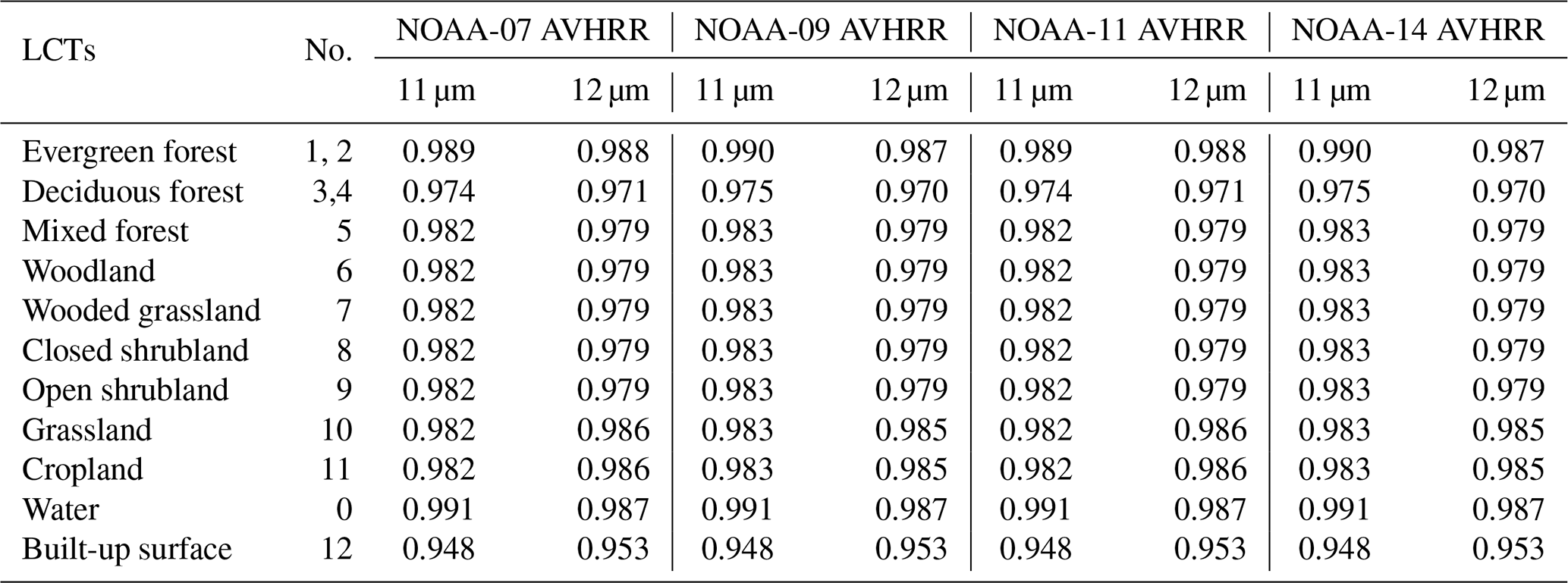
Figure 3 illustrates LSE estimation, which consists of two main parts.
The first part describes how static bare soil emissivity is obtained. After preparing the ASTER GED datasets, global mean NDVI and channel emissivity maps are obtained and mean fv is calculated via Eq. (3). In combination with the LUT for ASTER vegetation emissivity from Meng et al. (2016), an initial global ASTER bare soil emissivity map is obtained via Eq. (4). However, due to regions with persistent cloud cover and areas with dense vegetation (i.e., no visible bare soil fraction), the obtained global emissivity maps for bare soil still have considerable data gaps. These missing values in the bare soil emissivity maps are filled with the average emissivity of the same soil type within 3×3 neighborhood pixels. If there is no valid neighbor pixel for averaging, the neighborhood is enlarged until all data gaps are filled.
The second part describes the estimation of the daily dynamic emissivity. Firstly, the global ASTER background bare soil spectral channel emissivities are converted to AVHRR spectral channels via Eq. (5). Then, AVHRR channel emissivities are obtained via Eq. (2) with NDVI values from the AVH13C1 dataset. Vegetation emissivities are taken from a look-up table (Table 7), which is based on AVHRR LCTs and vegetation emissivities from Pinheiro et al. (2006). Furthermore, emissivities of built-up areas and water are used for separating these areas from other non-vegetated areas.
3.4 Orbital drift correction
The orbital drift of the NOAA-series satellites is a serious limitation for applications of AVHRR LST. Therefore, an orbital drift correction (ODC) would be highly useful and beneficial for many users. The actual overpass times of the NOAA-series afternoon satellites are between 13:00 and 17:30 ST. In order to include the four afternoon satellites (Table 1), the target time for ODC is set to 14:30 (solar time). According to the ODC method proposed by Liu et al. (2019a), the LST relationship between overpass time and ODC target time (14:30) can be written as follows:
where t is the time of the day in hours, Ta is the diurnal amplitude of LST in K, ω is the length of daytime, and tm is the time of maximum LST in hours (Göttsche and Olesen, 2001). Here, ω is determined by the duration of daytime: , where ϕ is the latitude of the pixel in degrees and δ is the solar declination. δ can be expressed as a function of the day of the year (DOY): (Elagib et al., 1998).
Similar to the component emissivity in Eq. (2), LST can be approximated as the weighted sum of the component temperatures of the vegetation and bare soil areas (Quan et al., 2018):
where Tveg and Tsoil are the component temperatures of vegetation and bare soil, respectively.
Starting with the approach by Liu et al. (2019a), we further divide the diurnal temperature amplitude Ta into two components (i.e., vegetation and soil). Thus, Eq. (6) can then be rewritten as follows:
where Ts,veg(14.5) and Ts,soil(14.5) are the component temperatures of vegetation and bare soil at target time 14:30 ST, respectively, and Ta,veg and Ta,soil are the components of diurnal temperature amplitude Ta, respectively.
In Eq. (8), the parameters Ts, fv, and t are available for each pixel. To obtain the other five parameters, Ts,veg(14.5), Ts,soil(14.5), Ta,veg, Ta,soil, and tm, it is assumed that the component temperatures and the shape of the diurnal temperature cycle are approximately the same in a 3×3 pixel neighborhood. With this assumption, there are nine equations to solve for the five unknown parameters. To constrain the solution, boundaries are set for each parameter. The boundaries for Ts,veg(14.5) and Ts,soil(14.5) are [Tcenter−10, Tcenter+15] K, and Tcenter is the LST for the center pixel in the 3×3 neighborhood. The boundaries for Ta,veg and Ta,soil are [5, 40] K and Ta,soil must be larger than Ta,veg. The boundary for tm is [12, 15] in hours. In order to obtain more stable parameters, the pixel's ODC parameters obtained with an averaged value from the neighborhood when Eq. (8) cannot be fitted, e.g., fv are similar to each other (e.g., fv=0, 1) in the 3×3 pixel neighborhood. If there is no valid neighbor pixel for averaging, the neighborhood area is enlarged from 3×3 to 9×9. Once the parameters are determined, the LST at 14:30 ST can be calculated via Eq. (9).
3.5 Generation of LST products
The product generation executable (PGE) code includes four modules. Module I is for generating the multi-LST with the selected SWAs. Three different types of input data enter this module: (i) the satellite data, i.e., BTs from AVH02C1, NDVI from AVH13C1, bare soil emissivity (see section 3.3), and AVHRR LCTs from UMD; (ii) look-up tables, i.e., coefficients of the SWAs (see Sect. 3.1) and emissivities of vegetation, water, and built-up areas (see Table 7); and (iii) ancillary data, i.e., NSAT and CWVC from MERRA and the land–sea mask. The QC flags in AVHR02C1 are also used to identify cloudy pixels. If a pixel contains cloud or cloud shadow, its LST is not calculated. Therefore, the output of Module I is multi-LST under clear sky conditions.
Module II is for integrating the multi-LST with the trained RF ensemble model. The inputs include the multi-LST from Module I and the RF ensemble model; the output is the ensemble LST, which is termed RF-SWA LST. Module III is for normalizing the LST affected by orbital drift to 14:30 ST. In this module, the input datasets include the RF-SWA LST and NDVI; the latter is used for calculating the fraction of vegetation. The output of Module III is orbital-drift-corrected LST, which is termed OCD LST. Module IV is for generating monthly average LST: the module first groups ODC LST by month, sums the valid LST in each month up, and then divides them by the respective number of valid LST. The output from this module is monthly averaged ODC LST. All LST data are stored in standard HDF-EOS format. Table 8 shows the variables provided in the three types of LST data files.
3.6 LST product validation based on in situ LST
At the surface, in situ LST can be estimated from measurements of broadband hemispherical upwelling radiance (Lu) and atmospheric downwelling radiance (Ld) using Stefan–Boltzmann's law:
where Ts is in situ LST, broadband emissivity ε is obtained from AVHRR LSE in AVHRR LSE for channel centered at 11 and 12 µm via the empirical relationship (Liang, 2005), and W (m2 K4)−1) is the Stefan–Boltzmann constant.
Before the validation was performed, in situ LST and AVHRR LST were accurately matched up in terms of geolocation and acquisition time (nearest-neighbor interpolation and, depending on the site, time differences of less than 3, 15 or 30 min). Furthermore, VZAs were limited to less than 40∘. Additionally, three-sigma (3σ) filtering (Eq. 11) was employed to remove the samples contaminated by undetected clouds (Göttsche et al., 2016; Pearson, 2002).
where xk is the LST differences between the retrieved and in situ values, and xmed is the median of the residuals. Matchups with residuals greater than xmed+3S or less than xmed−3S are regarded as outliers.
4.1 Training results and selection of SWAs
For NOAA-07/11 AVHRR, the candidate SWAs in Table 5 were already trained and evaluated by Zhou et al. (2019b). Here, the SWAs are additionally trained and evaluated for NOAA-09/14 AVHRR. Generally, the SWA training results for the four sensors are consistent with each other. Therefore, only the result for NOAA-14 AVHRR is listed here. The candidate algorithms OV1992, FO1996, and FOW 1996 show the worst regression accuracy regardless of atmospheric conditions, with standard errors of the estimate (SEE) higher than 1.49, 1.48, and 1.32 K, respectively. For Warm-ATM, the SEE of PP1991 increases rapidly with increasing CWVC, while it shows good accuracy for Cold-ATM with SEE between 0.33 and 0.75 K. The SEE values for UC1985 and MT2002 were larger than those of most other SWAs, even though they are still lower than for OV1992, FO1996, FOW1996, and PP1991. Therefore, these six SWAs were disregarded in the further analysis. For the remaining 11 SWAs, a sensitivity analysis was performed for the TRA-G simulation dataset with uncertainties levels L1 and L2. The results showed that SO1991 and CO1994 are sensitive to uncertainties in LSE and CWVC. Consequently, these two SWAs were also excluded from the candidate algorithm list. More details on the training and sensitivity analysis are provided in Zhou et al. (2019b).
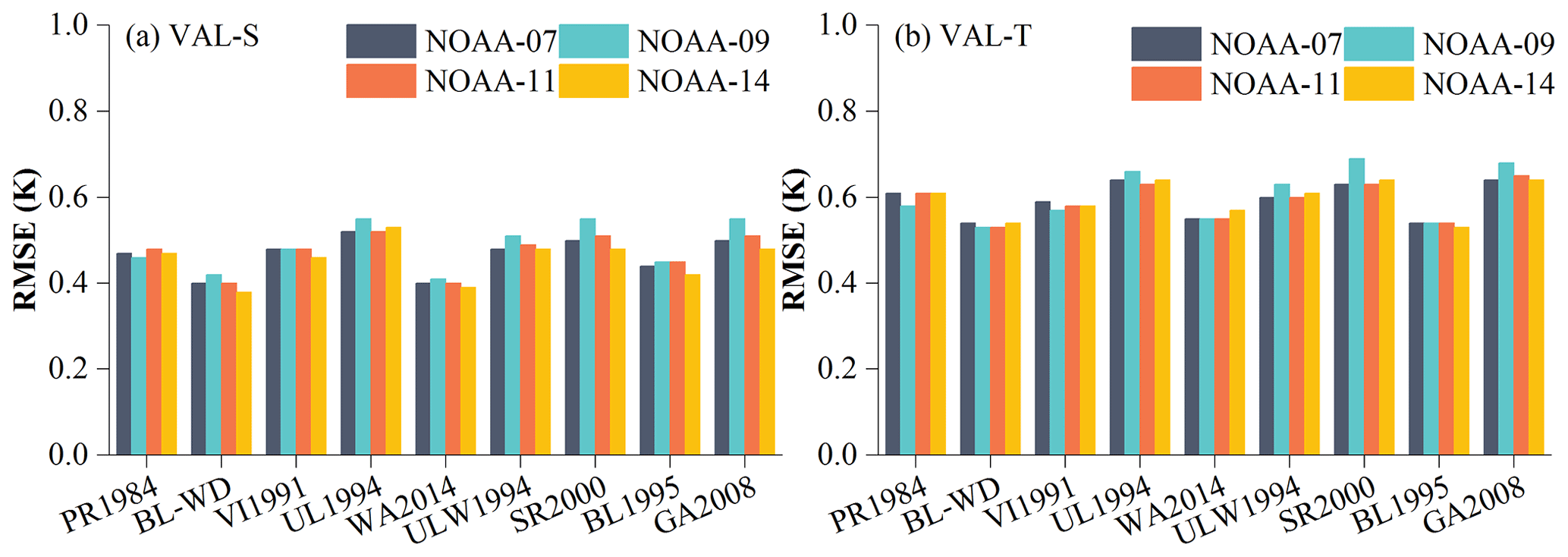
The nine remaining SWAs for NOAA-09/14 AVHRR were then tested with the simulation datasets VAL-S and VAL-T. For completeness, Fig. 4 shows these results together with those obtained for NOAA-07/11. It can be seen that the retained nine SWAs have low root-mean-square error (RMSE) values, which range between 0.38 and 0.49 K for VAL-S and between 0.47 and 0.68 K for VAL-T. Since the atmospheric profiles used to generate VAL-S and VAL-T are globally distributed, we conclude that these nine SWAs should perform well globally. The results for VAL-S in Fig. 4 reveal that BL-WD and WA2014 show the highest overall accuracy, followed by BL1995, PR1984, and VI1991. The RMSE values of these four SWAs are ∼ 0.48 K. For VAL-T, BL1995 and BL_WD show the highest accuracy, followed by WA2014, VI1991, and PR1984; in this case, the RMSE of these four SWAs is ∼ 0.60 K. For all nine SWAs, the accuracy decreases as the VZA increases. While BL-WD achieves the highest accuracy, no obvious differences between the other eight SWAs are observed. From the 17 LCTs over which the atmospheric profiles are located, taking VAL-T for NOAA-14 AVHRR as an example, BL-WD performs best for nine LCTs, and VI1991 and BL1995 perform best for three LCTs. In contrast, there is no LC type over which PR1984, SR2000, GA2008, and UL1994 perform best. It is because those SWAs show different sensitivity to the emissivity, which was set by the LCTs of profiles located. When assessing the effect of different atmospheric conditions, in Cold-ATM the highest accuracy is found for BL1995 and BL-WD. In Warm-ATM, when Ts-NSAT is within [−4, 20] K, BL-WD performs the best for CWVC below 2.5 g cm−2, while PR1984 performs the best when CWVC exceeds 4.5 g cm−2. When Ts-NSAT is within [−16,4] K, WA2014 shows the best performance for CWVC below 3.5 g cm−2. With increasing CWVC, BL1995 and BL-WD show the highest accuracy. Overall, it is found that no single SWA achieves the highest accuracy under all conditions.
4.2 Multi-LST ensemble
The nine SWAs were integrated with the RF ensemble method. For comparison, the simple averaging (SA) method and Bayesian model averaging (BMA) method were also employed. In contrast to Zhou et al. (2019b), here we used LST retrieved with SWAs trained with TRA-G (L0, L1, and L2) and VAL-S/T (L0) to simulate a more realistic situation with uncertainty. Generally, the mean bias error (MBE) of the RF ensemble method and the BMA model method is negligible (of the order of 10−4 K or less), while the MBE of SA method and single SWA is larger (of the order of 0.1 K). It can be concluded that the two ensemble methods (i.e., RF and BMA) similarly reduce systematic error. In terms of training accuracy, the RF model shows obvious advantages, with a standard deviation (SD) of less than 0.50 K for the four NOAA AVHRR sensors, while the SD of SA and BMA is larger and varies between 1.27 and 1.35 K. Figure 5 highlights the importance of variance for forming the RF ensemble: the most important SWA is BL1995, with an importance value of 0.67, 0.64, 0.68, and 0.83 for NOAA-07, 09, 11, and 14, respectively. The second most important SWA for NOAA-07, 09, and 11 is ULW1994, while WA2014 is the second most important SWA for NOAA-14. SR2000 is also of some importance for the ensemble process. Figure 5 confirms that the most important SWA, i.e., BL1995, is consistent with the most accurate SWA under different atmospheric conditions.
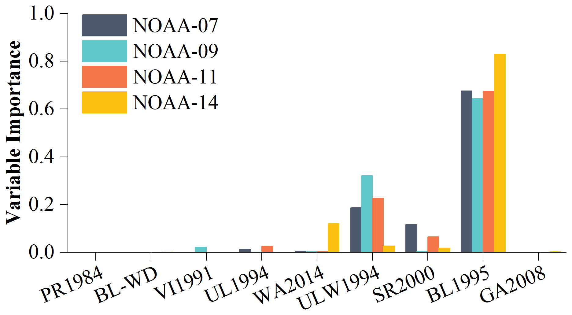

Figure 6SEE values of the three ensemble methods for NOAA-14 AVHRR under different atmospheric and VZA conditions. (a) Cold-ATM for Ts − NSAT within [−4, 20] K and [−16, 4] K. (b) Warm-ATM for Ts − NSAT within [−4, 20] K. (c) Warm-ATM for Ts − NSAT within [−16, 4] K.
Figure 6 shows the SEEs of the three ensemble methods for different CWVC zones and VZA subranges for NOAA-14 AVHRR. Compared to the BMA and SA models for all atmospheric conditions and VZAs, the RF ensemble model achieves an obvious improvement in LST accuracy. For Cold-ATM, the SEE of RF increases slowly with increasing CWVC and VZA and varies from 0.21 to 0.45 K. In contrast, the SEEs of BMA and SA show larger variations for both, increasing CWVC and VZA, and range from 0.72 to 1.23 K. For Warm-ATM and CWVC less than 3.0 g cm−2, there is no obvious increase in SEE with increasing CWVC or VZA. However, SEE increases noticeably with increasing VZA when CWVC exceeds 3.0 g cm−2, especially at VZA larger than 35∘. However, the SEE of RF is always smaller than that of BMA and SA: RF SEE only exceeds 1.0 K when CWVC is larger than 5.0 g cm−2 and VZA exceeds 60∘. Under the same conditions, the SEE of BMA and SA is larger than 2.0 K. Therefore, it is concluded that the RF ensemble method achieves a higher training accuracy than the BMA and SA methods, with a RF training accuracy of less than 1.0 K under most conditions.
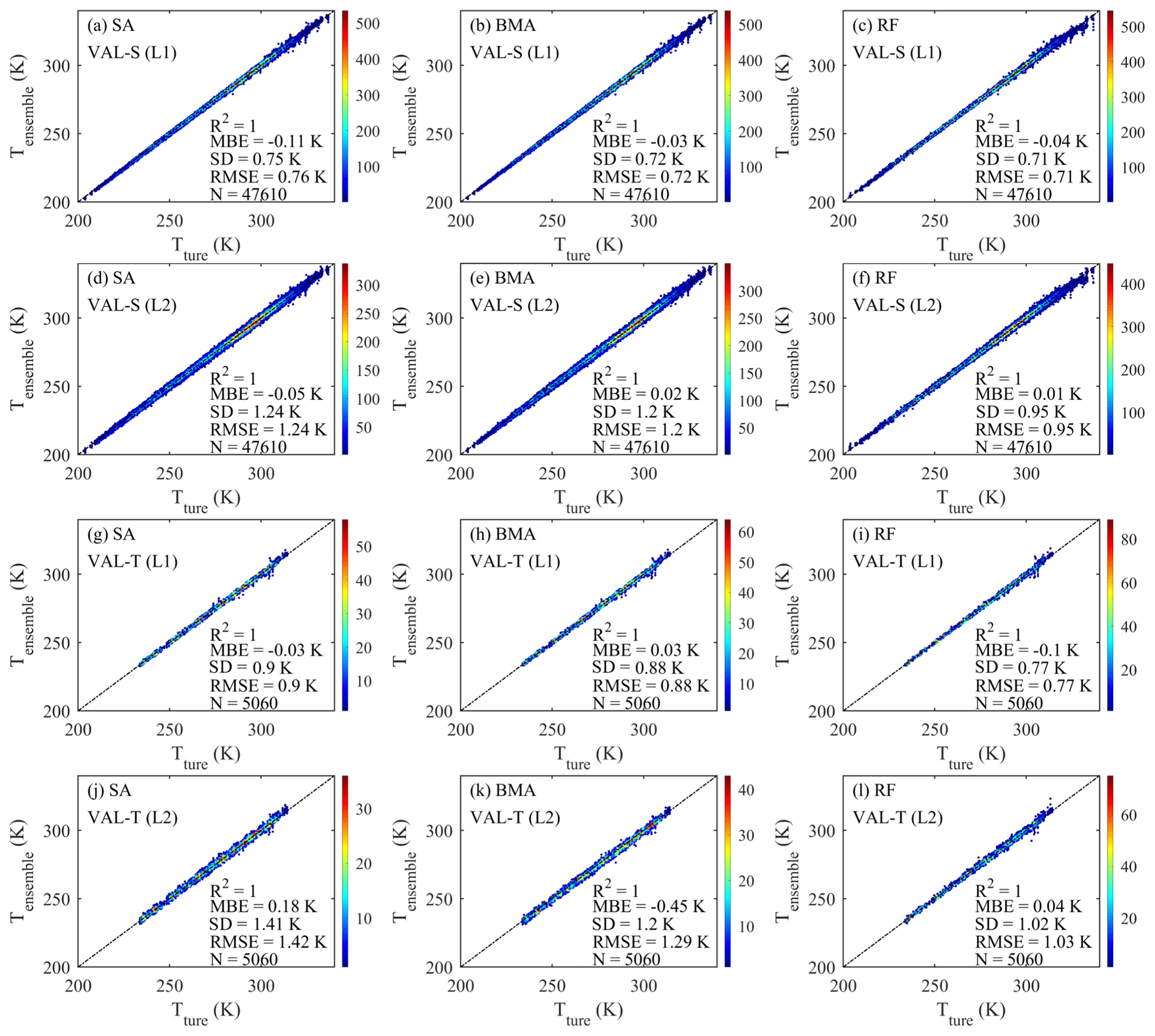
Figure 7LST retrieved with the three ensemble methods for NOAA-14 against true LST. Results are based on simulation datasets VAL-T and VAL-S with added Gaussian noise (uncertainty levels L1 and L2).
To assess the stability and sensitivity of the RF model, the LST estimated with RF, BMA, and SA methods was evaluated against the VAL-T and VAL-S datasets at uncertainty levels L1 and L2. Figure 7 shows the evaluation of the three methods for NOAA-14 AVHRR. For VAL-S at L1, SD and RMSE of about 0.7 K are found for all three methods; however, the biases of RF (MBE K) and BMA (MBE K) are smaller than that of SA (MBE K) and negligible (i.e., less than ±0.1 K). For VAL-S at L2, the bias for all three methods is negligible. However, considerable improvements are obtained with the RF method in terms of SD and RMSE, which is about 0.25K lower than for BMA and SA. For VAL-T at L1, the RF method has a slightly larger bias (MBE K) than the SA and BMA methods; however, its SD and RMSE are smaller. For VAL-T at L2, the three methods have a similar bias. However, RF has a significantly smaller SD and RMSE of 1.02 and 1.03 K than SA (1.41 and 1.42 K) and BMA (1.38 and 1.39 K). Similar results were found for NOAA-07/09/11 AVHRR.
4.3 Validation of RF-SWA LST against in situ LST
First, the generated RF-SWA LST was validated against in situ LST from SURFRAD sites. Figure 8 shows a scatterplot between RF-SWA LST and SURFRAD in situ LST and some statistical indicators, i.e., MBE, RMSE, SD, R2, and N (i.e., sample size). High correlations are found between RF-SWA LST and in situ LST with a R2 range of 0.91–0.96. MBE varies between −1.59 and 2.71 K, and RMSE varies between 2.25 and 3.86 K. Compared to LST products for MODIS, AATSR, and VIIRS, which were also validated against SURFRAD in situ LST (Duan et al., 2019; Liu et al., 2019b; Martin et al., 2019), RF-SWA LST shows a similar accuracy and precision. It should be noted that the large MBE at BND, GWN, and TBL are probably due to a lack of in situ LST representativeness at the satellite scale, e.g., BND, a seasonal bias variation is observed. During the dormancy season, the surface within the ground radiometer's FOV and the corresponding AVHRR pixel are both fairly homogeneously covered by bare soil and grassland, which leads to smaller LST differences. In contrast, during the growing season, most of the area within the AVHRR pixel is covered by cropland and the fraction of vegetation cover depends on the crop's growth stage: especially in the early growing and harvesting season, there are many bare areas between crop rows, which causes larger LST differences. If only BND matchups during the dormancy season are considered, the corresponding MBE and RMSE between RF-SWA LST and in situ LST reduce to 1.56 and 2.58 K, respectively. At GWN, the land cover within the ground radiometer's FOV is also grassland; however, the corresponding AVHRR pixel includes several nearby forest areas. Therefore, the daytime LST observed on the pixel scale tends to be lower than the in situ LST. At TBL, RF-SWA LST is lower than in situ LST for in situ LST larger than 300 K: this may be explained by a larger vegetation area southeast of the site, which is included in the AVHRR pixel, while the ground radiometer's entire FOV is covered by bare soil.
Figure 9 shows scatterplots between RF-SWA LST and NDBC lake surface water temperature (LSWT) and some statistical indicators for buoys in the eastern Pacific, the Great Lakes, the Gulf of Mexico, and the western Atlantic. As shown in Table 4, the number of buoys for each area differs. The RF-SWA LST shows a good correlation with in situ LSWT, with R2 ranging from 0.94 to 0.98. The plots also show low systematic errors and high precision, e.g., MBEs are less than 0.26 K and RMSE ranges from 0.77 to 0.89 K. Overall, the validation results resemble those obtained for the simulation datasets in Sect. 4.2. Furthermore, the validation results meet WMO's requirements for applications of LST/LSWT in different fields, e.g., an uncertainty of 2.0 K for agricultural meteorology and of 1.0 K for climate monitoring (WMO, 2020).
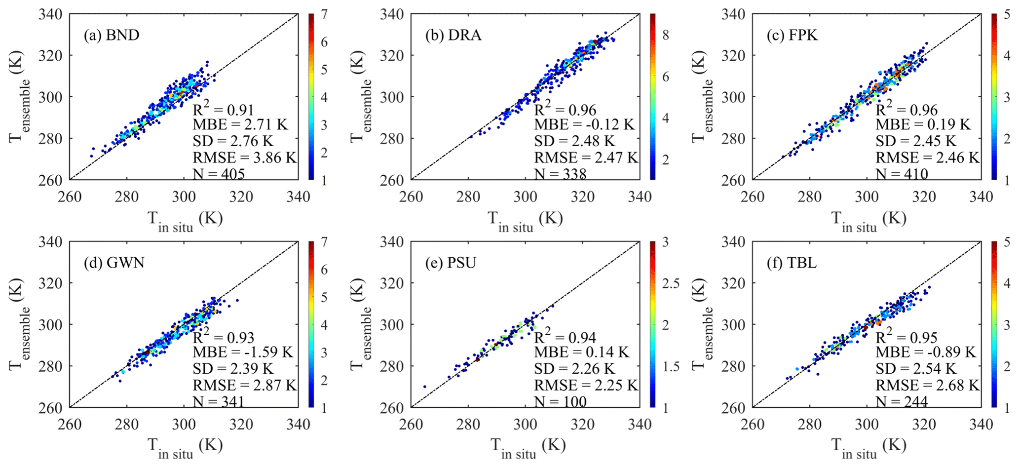
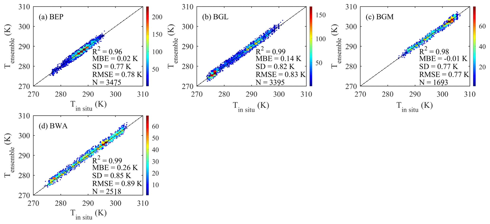
Figure 9RF-SWA LST against in situ LSWT from four NDBC sites (buoy data) and corresponding statistics.

Figure 10Residuals with respect to in situ LST for ODC and RF-SWA LST for six SURFRAD sites (BND, DRA, FPK, GWN, PSU, and TBL). Details about the sites are provided in Table 4.

Figure 11Monthly averaged ODC LST retrieved from NOAA-14 data for 1999 normalized to 14:30 ST: (a) March, (b) June, (c) September, (d) December.
4.4 Orbital drift correction
The retrieved RF-SWA LST were normalized for the orbital drift of the NOAA-series satellites using the orbital drift correction method described in Sect. 3.4. Since water surface temperature varies relatively slowly, only the retrieved surface temperatures over land were normalized. The orbital drift corrected LST (ODC LST) was then validated against the same in situ data as in Sect. 4.3. Figure 10 shows a boxplot of the residuals (TAVHRR−Tin situ) for the ODC LST and RF-SWA LST. The plot shows that the bias of the ODC LST over the six sites is similar to that of the uncorrected RF-SWA LST. From the six SURFRAD sites, BND has the highest positive bias, while GWN and TBL show negative biases. Following the explanation in Sect. 4.3, this is probably due to less representative in situ measurements. The standard deviations (SD) of the ODC LST residuals at the six SURFRAD sites are 3.62 K (BND), 2.34 K (DRA), 3.38 K (FPK), 3.45 K (GWN), 2.57 K (PSU), and 3.69 K (TBL). The SD variations (ODC LST–RF-SWA LST) range from 0.06 to 1.15 K. This indicates that the ODC LST maintains the good accuracy of RF-SWA LST and its performance primarily depends on surface conditions. This is understandable because the improved ODC method uses adjacent pixels to compensate for the lack of temporal information. Nevertheless, the improved ODC method provides a practical way to correct the effect of orbital drift on LST retrieved from NOAA AVHRR data.
4.5 Global ODC LST product examples
Figure 11 shows monthly averaged ODC LST for March, June, September, and December 1999 normalized to 14:30 ST. The LST show an obvious annual variation as seasons change with Earth's revolution around the Sun. In March and September (Fig. 11a and c), the Sun is overhead near the Equator, which then receives most of the solar energy. However, the highest LST are observed north and south of the Equator, i.e., over the Sahara and Australia. This is due to the equatorial regions' dense coverage with tropical rainforests, e.g., in the Amazon and Congo basins. The lowest LST are observed in the northern hemisphere around 45∘ N and around the Tibetan Plateau. In June (Fig. 11b), the Sun is more overhead in the Northern Hemisphere and the area with the highest LST is located around 30∘ N, i.e., over the Sahara, the Arabian Peninsula, and the Iran–Pamir Plateau. At the same time, LST also increases north of 45∘ N. In December (Fig. 11d), the area with the highest LST is mainly located over Oceania and parts of South America. It should be noted that the large areas with invalid data, which are mainly observed at latitudes larger than 45∘, are caused by the strict cloud filtering algorithms, which frequently recognize snow and ice as cloud, and polar night when no visible data are available to calculate NDVI (related to LSE). Furthermore, in June there are many invalid pixels over southern and southwestern China, an area regularly affected by cloudy weather.
In order to demonstrate the temporal consistency between satellites, Fig. 12 shows time series of monthly averaged ODC LST from 1981 to 2000 for the Amazon basin, the Arctic pole, and the Tibetan Plateau (areas are shown in Fig. 1): no significant orbital drift or inconsistencies can be seen, indicating that the ODC method adequately normalized the retrieved AVHRR LST. The larger annual variations over the north pole (Fig. 12b) are related to the specific variation of solar radiation in high-latitude areas, i.e., polar day and polar night. For the Amazon basin (Fig. 12a), the north Arctic pole (Fig. 12b), and the Tibetan Plateau (Fig. 12c), the linear regressions (blue lines) show different trends with rates of 0.048±0.024 K yr−1 (p value = 0.046), 0.087±0.221 K yr−1 (p value = 0.695), and 0.081±0.103 K yr−1 (p value = 0.433), respectively. However, these rates may be affected by averaging over large areas and by the frequently missing data due to clouds. Therefore, more in-depth analyses, especially with in situ observations and reanalysis data, are needed (Liu et al., 2008; Rigor et al., 2000; Schneider and Hook, 2010; Wu et al., 2013).
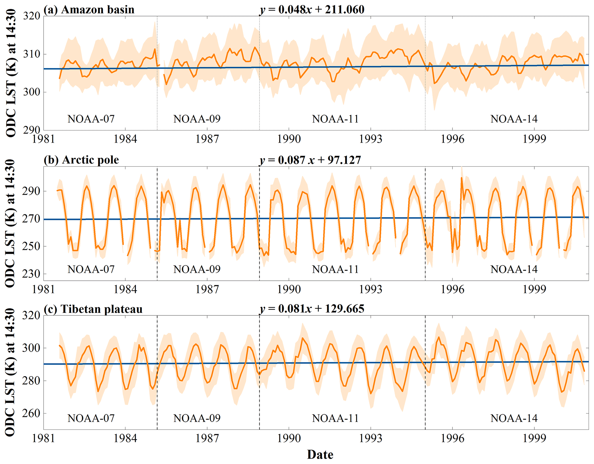
Figure 12Monthly averaged ODC LST time series normalized to 14:30 ST for 1981–2000 over the Amazon basin (a), the north pole (b), and the Tibetan Plateau (c).
Global LST products retrieved from NOAA/AVHRR data between 1981 to 2000 are freely available at https://doi.org/10.5281/zenodo.3934354 for RF-SWA LST (Ma et al., 2020a); https://doi.org/10.5281/zenodo.3936627 for ODC LST (Ma et al., 2020c); and https://doi.org/10.5281/zenodo.3936641 for monthly averaged LST (Ma et al., 2020b). The dataset is also available at the National Earth System Science Data Center, National Science & Technology Infrastructure of China (http://www.geodata.cn/thematicView/GLASS.html, last access: 2 December 2020) and the University of Maryland (http://glass.umd.edu/LST/, last access: 2 December 2020).
The NOAA AVHRR data were downloaded from Level-1 and Atmosphere Archive & Distribution System Distributed Active Archive Center (https://ladsweb.modaps.eosdis.nasa.gov/, last access: 2 December 2020, NASA, 2020). SURFRAD data were downloaded from ftp://aftp.cmdl.noaa.gov/data/radiation/surfrad/ (last access: 2 December 2020, NOAA, 2020a). BUOYS data were downloaded from the National Data Buoy Center (https://www.ndbc.noaa.gov/historical_data.shtml, last access: 2 December 2020, NOAA, 2020b).
Three global LST products with a spatial resolution of have been generated from historical NOAA-9, 11, and 14 AVHRR data (1981–2000). These LST products are obtained in four steps: (1) training and evaluation of 17 AVHRR SWAs, (2) integrating nine selected SWAs with the random forest method (RF-SWA), (3) correcting the effect of orbital drift by normalizing RF-SWA LST to 14:30 ST, and (4) validating the retrieved LST against in situ LST data.
The 17 trained candidate SWAs generally showed consistent results for the four sensors. The candidate algorithms OV1992, FO1996, FOW1996, PP1991, UC1985, and MT2002 had larger SEE than the other SWAs, while SO1991 and CO1994 were sensitive to uncertainties in LSE and CWVC. Therefore, these SWAs were rejected. The nine remaining SWAs were evaluated based on the simulation datasets VAL-S and VAL-T. The results show that the trained nine SWAs have RMSEs ranging between 0.38 and 0.55 K for VAL-S and between 0.53 and 0.69 K for VAL-T. Since the atmospheric profiles used to simulate and evaluate were chosen to be globally representative, we conclude that these nine SWAs should perform well globally.
The RF ensemble method was then applied to the nine selected SWAs. Compared to individual SWAs, sample averaging, and the BMA ensemble method, the RF ensemble method showed the best accuracy when evaluated against the simulation datasets. The RF ensemble algorithm yielded an accuracy better than 0.8 K for a maximum LSE uncertainty of 0.02 and a maximum CWVC uncertainty of 1.0 g cm−2; the accuracy was still better than 1.10 K when the maximum LSE uncertainty increased to 0.04. Based on these results, the algorithm theoretically satisfies the target accuracy requirement of WMO, i.e., an accuracy better than 1.0 K at a spatial resolution of 5 km. Furthermore, it is concluded that the RF method outperforms the SA and BMA methods and has the greatest potential for improving LST retrieval accuracy.
The RF-SWA LST and ODC LST are validated against in situ LST from SURFRAD sites and NDBC buoys. Against SURFRAD LST, the MBE of RF-SWA LST varies from −1.59 to 2.71 K and its SD varies from 2.26 to 2.76 K, which is similar to LST products retrieved from other sensors, e.g., MODIS. Against NDBC data from 1981 to 2000, RF-SWA LST also shows good accuracy and precision: with its small MBE (less than 0.10 K) and a SD ranging from 0.84 to 1.05 K, its performance against in situ water temperature is similar to that for the simulated datasets. When validated against the same SURFRAD LST, the MBE of ODC LST ranges from −1.05 to 3.01 K, which is similar to the MBE obtained for RF-SWA LST; its SD increases and ranges from 2.34 to 3.69 K. Overall, it is concluded that both RF-SWA LST and ODC LST achieve similar accuracy.
The generated global AVHRR LST is well suited to meet the needs of many applications and studies, e.g., understanding global climate change, radiation budgeting, energy balancing, and mapping of land cover change. However, further research should address the following points: first, the developed LST products were validated against in situ LST data from North America, while they need to be validated globally, e.g., against AsiaFlux measurements, historical air temperature, reanalysis data, etc. Second, ODC LST is obtained at a single overpass time, which required using prior knowledge on temporal parameters. If additional information on LST would be available, e.g., from modeling datasets, geostationary satellite datasets, and AVHRR nighttime datasets, it could improve future research. Third, over some areas, there are many invalid values, e.g., southwestern China, which frequently experiences cloudy and rainy weather. It is expected that future work can utilize recent progress in generating global all-weather LST products (Martins et al., 2019; Zhang et al., 2020) to help integrate multi-source data, e.g., passive microwave brightness temperature and reanalysis data.
JM and JZ designed the research, and JM implemented the research and completed the original manuscript. JZ and FMG supervised the research. SL founded and improved the research. SW and ML assisted in generating the RF-SWA LST and ODC LST, respectively. All co-authors revised the manuscript and contributed to the writing.
The authors declare that they have no conflict of interest.
We would like to thank the editor and the two anonymous referees for their valuable comments. We would also like to thank all colleagues who helped with data processing and suggestions. Jin Ma also thanks the China Scholarship Council for his stay at the Karlsruhe Institute of Technology, Germany.
This research has been supported by the National Key Research and Development Program of China (grant no. 2018YKF1505205), the National Natural Science Foundation of China (grant no. 41871241), the Fundamental Research Funds of the Central Universities of China (grant no. ZYGX2019J069), and the China Scholarship Council (grant no. 201906070077).
This paper was edited by Ge Peng and reviewed by two anonymous referees.
Aires, F., Prigent, C., Rossow, W. B., and Rothstein, M.: A new neural network approach including first guess for retrieval of atmospheric water vapor, cloud liquid water path, surface temperature, and emissivities over land from satellite microwave observations, J. Geophys. Res.-Atmos., 106, 14887–14907, https://doi.org/10.1029/2001JD900085, 2001.
Anderson, M. C., Kustas, W. P., Norman, J. M., Hain, C. R., Mecikalski, J. R., Schultz, L., González-Dugo, M. P., Cammalleri, C., d'Urso, G., Pimstein, A., and Gao, F.: Mapping daily evapotranspiration at field to continental scales using geostationary and polar orbiting satellite imagery, Hydrol. Earth Syst. Sci., 15, 223–239, https://doi.org/10.5194/hess-15-223-2011, 2011.
Bechtel, B.: Robustness of annual cycle parameters to characterize the urban thermal landscapes, IEEE Geosci. Remote Sens. Lett., 9, 876–880, https://doi.org/10.1109/LGRS.2012.2185034, 2012.
Becker, F. and Li, Z.-L.: Towards a local split window method over land surfaces, Int. J. Remote Sens., 11, 369–393, https://doi.org/10.1080/01431169008955028, 1990a.
Becker, F. and Li, Z.-L.: Surface temperature and emissivity at various scales: definition, measurement and related problems, Remote Sens. Rev., 12, 225–253, https://doi.org/10.1080/02757259509532286, 1995.
Becker, F. and Li, Z. L.: Temperature-independent spectral indices in thermal infrared bands, Remote Sens. Environ., 32, 17–33, https://doi.org/10.1016/0034-4257(90)90095-4, 1990b.
Berk, A., Anderson, G. P., Acharya, P. K., Bernstein, L. S., Muratov, L., Lee, J., Fox, M., Adler-Golden, S. M., Chetwynd, J. H., Hoke, M. L., Lockwood, R. B., Gardner, J. A., Cooley, T. W., Borel, C. C., and Lewis, P. E.: MODTRAN 5: a reformulated atmospheric band model with auxiliary species and practical multiple scattering options: update, Proceedings Volume 5806, Algorithms and Technologies for Multispectral, Hyperspectral, and Ultraspectral Imagery XI, https://doi.org/10.1117/12.606026, 2005.
Borbas, E., Seemann, S. W., Huang, H.-L., Li, J., and Menzel, W. P.: Global profile training database for satellite regression retrievals with estimates of skin temperature and emissivity, Int. ATOVS Study Conf., 763–770, 2005.
Breiman, L.: Random forests, Mach. Learn., 45, 5–32, 2001.
Carlson, T. N. and Ripley, D. A.: On the relation between NDVI, fractional vegetation cover, and leaf area index, Remote Sens. Environ., 62, 241–252, https://doi.org/10.1016/S0034-4257(97)00104-1, 1997.
Casey, K. S., Brandon, T. B., Cornillon, P., and Evans, R.: The Past, Present, and Future of the AVHRR Pathfinder SST Program BT – Oceanography from Space: Revisited, edited by: Barale, V., Gower, J. F. R., and Alberotanza, L., Springer Netherlands, Dordrecht, 273–287, 2010.
Chedin, A., Scott, N. A., Wahiche, C., and Moulinier, P.: The Improved Initialization Inversion Method: A High Resolution Physical Method for Temperature Retrievals from Satellites of the TIROS-N Series, J. Clim. Appl. Meteorol., 24, 128–143, https://doi.org/10.1175/1520-0450(1985)024<0128:TIIIMA>2.0.CO;2, 1985.
Choi, Y.-Y. and Suh, M.-S.: Development of Himawari-8/Advanced Himawari Imager (AHI) Land Surface Temperature Retrieval Algorithm, Remote Sens., 10, 2013, https://doi.org/10.3390/rs10122013, 2018.
Coll, C., Caselles, V., Sobrino, J. A., and Valor, E.: On the atmospheric dependence of the split-window equation for land surface temperature, Int. J. Remote Sens., 15, 105–122, https://doi.org/10.1080/01431169408954054, 1994.
Dech, S., Tungalagsaikhan, P., Preusser, C., and Meisner, R.: Operational value-adding to AVHRR data over Europe: methods, results, and prospects, Aero. Sci. Technol., 2, 335–346, https://doi.org/10.1016/S1270-9638(98)80009-6, 1998.
Defries, R. S. and Hansen, M. C.: ISLSCP II University of Maryland Global Land Cover Classifications, 1992–1993, ORNL DAAC, Oak Ridge, Tennessee, USA, https://doi.org/10.3334/ORNLDAAC/969, 2010.
Dong, L., Yang, H., Zhang, P., Tang, S., and Lu, Q.: Retrieval of Land Surface Temperature and Dynamic Monitoring of a High Temperature Weather Process Based on FY-3A/VIRR Data, J. Appl. Meteorol. Sci., 23, 214–222, 2012.
Duan, S.-B., Li, Z.-L., Li, H., Göttsche, F.-M., Wu, H., Zhao, W., Leng, P., Zhang, X., and Coll, C.: Validation of Collection 6 MODIS land surface temperature product using in situ measurements, Remote Sens. Environ., 225, 16–29, https://doi.org/10.1016/j.rse.2019.02.020, 2019.
Duguay-Tetzlaff, A., Bento, V. A., Göttsche, F. M., Stöckli, R., Martins, J. P. A., Trigo, I., Olesen, F., Bojanowski, J. S., da Camara, C., and Kunz, H.: Meteosat land surface temperature climate data record: Achievable accuracy and potential uncertainties, Remote Sens., 7, 13139–13156, https://doi.org/10.3390/rs71013139, 2015.
Elagib, N. A., Alvi, S. H., and Mansell, M. G.: Day-length and extraterrestrial radiation for Sudan: A comparative study, Int. J. Sol. Energy, 20, 93–109, https://doi.org/10.1080/01425919908914348, 1998.
Fang, H., Beaudoing, H. K., Rodell, M., Teng, W. L., and Vollmer, B. E.: Global Land Data Assimilation System (GLDAS) products, services and application from NASA Hydrology Data and Information Services Center (HDISC), ASPRS 2009 Annual Conference, Baltimore, Maryland, 8–13 March 2009, 151–159, 2009.
Francois, C. and Ottle, C.: Atmospheric corrections in the thermal infrared: global and water vapor dependent split-window algorithms-applications to ATSR and AVHRR data, IEEE Trans. Geosci. Remote Sens., 34, 457–470, https://doi.org/10.1109/36.485123, 1996.
Galve, J. M., Coll, C., Caselles, V., and Valor, E.: An Atmospheric Radiosounding Database for Generating Land Surface Temperature Algorithms, IEEE Trans. Geosci. Remote Sens., 46, 1547–1557, https://doi.org/10.1109/TGRS.2008.916084, 2008.
Ghent, D. J., Corlett, G. K., Göttsche, F. M., and Remedios, J. J.: Global Land Surface Temperature From the Along-Track Scanning Radiometers, J. Geophys. Res.-Atmos., 122, 12167–12193, https://doi.org/10.1002/2017JD027161, 2017.
Gillespie, A., Rokugawa, S., Matsunaga, T., Cothern, J. S., Hook, S., and Kahle, A. B.: A temperature and emissivity separation algorithm for Advanced Spaceborne Thermal Emission and Reflection Radiometer (ASTER) images, IEEE Trans. Geosci. Remote Sens., 36, 1113–1126, https://doi.org/10.1109/36.700995, 1998.
Gleason, A. C. R., Prince, S. D., Goetz, S. J., and Small, J.: Effects of orbital drift on land surface temperature measured by AVHRR thermal sensors, Remote Sens. Environ., 79, 147–165, https://doi.org/10.1016/S0034-4257(01)00269-3, 2002.
Göttsche, F.-M., Olesen, F.-S., Trigo, I., Bork-Unkelbach, A., and Martin, M.: Long Term Validation of Land Surface Temperature Retrieved from MSG/SEVIRI with Continuous in-Situ Measurements in Africa, Remote Sens., 8, 410, https://doi.org/10.3390/rs8050410, 2016.
Göttsche, F. M. and Olesen, F. S.: Modelling of diurnal cycles of brightness temperature extracted from meteosat data, Remote Sens. Environ., 76, 337–348, https://doi.org/10.1016/S0034-4257(00)00214-5, 2001.
Guillevic, P. C., Biard, J. C., Hulley, G. C., Privette, J. L., Hook, S. J., Olioso, A., Göttsche, F. M., Radocinski, R., Román, M. O., Yu, Y., and Csiszar, I.: Validation of Land Surface Temperature products derived from the Visible Infrared Imaging Radiometer Suite (VIIRS) using ground-based and heritage satellite measurements, Remote Sens. Environ., 154, 19–37, https://doi.org/10.1016/j.rse.2014.08.013, 2014.
Gutman, G. G.: On the monitoring of land surface temperatures with the NOAA/AVHRR: Removing the effect of satellite orbit drift, Int. J. Remote Sens., 20, 3407–3413, https://doi.org/10.1080/014311699211435, 1999.
Holmes, T. R. H., De Jeu, R. A. M., Owe, M., and Dolman, A. J.: Land surface temperature from Ka band (37 GHz) passive microwave observations, J. Geophys. Res.-Atmos., 114, D04113, https://doi.org/10.1029/2008JD010257, 2009.
Huang, F., Zhou, J., Tao, J., Tan, X., Liang, S., and Cheng, J.: PMODTRAN: a parallel implementation based on MODTRAN for massive remote sensing data processing, Int. J. Digit. Earth, 9, 819–834, https://doi.org/10.1080/17538947.2016.1144800, 2016.
Hulley, G. C. and Hook, S. J.: Generating consistent land surface temperature and emissivity products between ASTER and MODIS data for earth science research, IEEE Trans. Geosci. Remote Sens., 49, 1304–1315, https://doi.org/10.1109/TGRS.2010.2063034, 2011.
Hulley, G. C., Hook, S. J., Abbott, E., Malakar, N., Islam, T., and Abrams, M.: The ASTER Global Emissivity Dataset (ASTER GED): Mapping Earth's emissivity at 100 meter spatial scale, Geophys. Res. Lett., 42, 7966–7976, https://doi.org/10.1002/2015GL065564, 2015.
Hutengs, C. and Vohland, M.: Downscaling land surface temperatures at regional scales with random forest regression, Remote Sens. Environ., 178, 127–141, https://doi.org/10.1016/j.rse.2016.03.006, 2016.
IPCC: Climate Change 2014: Synthesis Report, Contribution of Working Groups I, II and III to the Fifth Assessment Report of the Intergovernmental Panel on Climate Change, 2014.
Jiang, G. M. and Liu, R.: Retrieval of sea and land surface temperature from SVISSR/FY-2C/D/E measurements, IEEE Trans. Geosci. Remote Sens., 52, 6132–6140, https://doi.org/10.1109/TGRS.2013.2295260, 2014.
Jiménez, C., Prigent, C., Ermida, S. L., and Moncet, J.-L.: Inversion of AMSR-E observations for land surface temperature estimation: 1. Methodology and evaluation with station temperature, J. Geophys. Res.-Atmos., 122, 3330–3347, https://doi.org/10.1002/2016JD026144, 2017.
Jin, M. and Dickinson, R. E.: New observational evidence for global warming from satellite, Geophys. Res. Lett., 29, 39-1–39-4, https://doi.org/10.1029/2001GL013833, 2002.
Jin, M. and Treadon, R. E.: Correcting the orbit drift effect on AVHRR land surface skin temperature measurements, Int. J. Remote Sens., 24, 4543–4558, https://doi.org/10.1080/0143116031000095943, 2003.
Julien, Y. and Sobrino, J. A.: Correcting AVHRR Long Term Data Record V3 estimated LST from orbital drift effects, Remote Sens. Environ., 123, 207–219, https://doi.org/10.1016/j.rse.2012.03.016, 2012.
Lembrechts, J. J., Lenoir, J., Roth, N., Hattab, T., Milbau, A., Haider, S., Pellissier, L., Pauchard, A., Ratier Backes, A., Dimarco, R. D., Nuñez, M. A., Aalto, J., and Nijs, I.: Comparing temperature data sources for use in species distribution models: From in-situ logging to remote sensing, Glob. Ecol. Biogeogr., 28, 1578–1596, https://doi.org/10.1111/geb.12974, 2019.
Li, Z.-L., Tang, B.-H., Wu, H., Ren, H., Yan, G., Wan, Z., Trigo, I. F., and Sobrino, J. A.: Satellite-derived land surface temperature: Current status and perspectives, Remote Sens. Environ., 131, 14–37, https://doi.org/10.1016/j.rse.2012.12.008, 2013a.
Li, Z. L., Wu, H., Wang, N., Qiu, S., Sobrino, J. A., Wan, Z., Tang, B. H., and Yan, G.: Land surface emissivity retrieval from satellite data, Int. J. Remote Sens., 34, 3084–3127, https://doi.org/10.1080/01431161.2012.716540, 2013b.
Liang, S.: Estimation of Surface Radiation Budget: I. Broadband Albedo, in Quantitative Remote Sensing of Land Surfaces, John Wiley & Sons, Inc., Hoboken, NJ, USA, 310–344, 2005.
Liang, S., Cheng, J., Jia, K., Jiang, B., Liu, Q., Xiao, Z., Yao, Y., Yuan, W., Zhang, X., Zhao, X., and Zhou, J.: The Global LAnd Surface Satellite (GLASS) product suite, B. Am. Meteorol. Soc., 1–37, https://doi.org/10.1175/BAMS-D-18-0341.1, online first, 2020.
Liu, X., Tang, B. H., Yan, G., Li, Z. L., and Liang, S.: Retrieval of global orbit drift corrected land surface temperature from long-term AVHRR data, Remote Sens., 11, 2843, https://doi.org/10.3390/rs11232843, 2019a.
Liu, Y., Key, J. R., and Wang, X.: The influence of changes in cloud cover on recent surface temperature trends in the Arctic, J. Clim., 21, 705–715, https://doi.org/10.1175/2007JCLI1681.1, 2008.
Liu, Y., Yu, Y., Yu, P., Wang, H., and Rao, Y.: Enterprise LST Algorithm Development and Its Evaluation with NOAA 20 Data, Remote Sens., 11, 2003, https://doi.org/10.3390/rs11172003, 2019b.
Llewellyn-Jones, D. T., Minnett, P. J., Saunders, R. W., and Zavody, A. M.: Satellite multichannel infrared measurements of sea surface temperature of the N.E. Atlantic Ocean using AVHRR/2, Q. J. Roy. Meteor. Soc., 110, 613–631, https://doi.org/10.1002/qj.49711046504, 1984.
Ma, J., Zhou, J., Göttsche, F.-M., Liang, S., and Wang, S.: GLASS Land Surface Temperature product (1981–2000): instantaneous LST, Zenodo, https://doi.org/10.5281/zenodo.3934354, 2020a.
Ma, J., Zhou, J., and Liang, S.: GLASS Land Surface Temperature product (1981–2000): monthly averaged LST, Zenodo, https://doi.org/10.5281/zenodo.3936641, 2020b.
Ma, J., Zhou, J., Liang, S., and Li, M.: GLASS Land Surface Temperature product (1981–2000): Orbital Drift Corrected LST, Zenodo, https://doi.org/10.5281/zenodo.3936627, 2020c.
Ma, Y. and Tsukamoto, O.: Combining Satellite Remote Sensing With Field Observations for Land Surface Heat Fluxes Over Inhomogeneous Landscape, China Meteorol, China Meteorological Press, Beijing, 2002.
Martin, M., Ghent, D., Pires, A., Göttsche, F.-M., Cermak, J., and Remedios, J.: Comprehensive In Situ Validation of Five Satellite Land Surface Temperature Data Sets over Multiple Stations and Years, Remote Sens., 11, 479, https://doi.org/10.3390/rs11050479, 2019.
Martins, J. P. A., Trigo, I. F., Ghilain, N., Jimenez, C., Göttsche, F. M., Ermida, S. L., Olesen, F. S., Gellens-Meulenberghs, F., and Arboleda, A.: An all-weather land surface temperature product based on MSG/SEVIRI observations, Remote Sens., 11, 3044, https://doi.org/10.3390/rs11243044, 2019.
Masiello, G., Serio, C., Venafra, S., Liuzzi, G., Göttsche, F., F. Trigo, I., and Watts, P.: Kalman filter physical retrieval of surface emissivity and temperature from SEVIRI infrared channels: a validation and intercomparison study, Atmos. Meas. Tech., 8, 2981–2997, https://doi.org/10.5194/amt-8-2981-2015, 2015.
McMillin, L. M.: Estimation of sea surface temperatures from two infrared window measurements with different absorption, J. Geophys. Res., 80, 5113–5117, https://doi.org/10.1029/jc080i036p05113, 1975.
Meng, X., Li, H., Du, Y., Cao, B., Liu, Q., Sun, L., and Zhu, J.: Estimating land surface emissivity from ASTER GED products, J. Remote Sens., 4619, 382–396, 2016.
Mutanga, O., Adam, E., and Cho, M. A.: High density biomass estimation for wetland vegetation using worldview-2 imagery and random forest regression algorithm, Int. J. Appl. Earth Obs. Geoinf., 18, 399–406, https://doi.org/10.1016/j.jag.2012.03.012, 2012.
NASA: Level-1 and Atmosphere Archive & Distribution System Distributed Active Archive Center, available at: https://ladsweb.modaps.eosdis.nasa.gov/, last access: 2 December 2020.
Niclòs, R., Caselles, V., Coll, C., and Valor, E.: Determination of sea surface temperature at large observation angles using an angular and emissivity-dependent split-window equation, Remote Sens. Environ., 111, 107–121, https://doi.org/10.1016/j.rse.2007.03.014, 2007.
National Oceanic & Atmospheric Administration (NOAA): ESRL Global Monitoring Laboratory: SURFRAD (Surface Radiation Budget) Network, available at: ftp://aftp.cmdl.noaa.gov/data/radiation/surfrad/, last access: 2 December 2020a.
National Oceanic & Atmospheric Administration (NOAA): National Data Buoy Center, available at: https://www.ndbc.noaa.gov/historical_data.shtml, last access: 2 December 2020b.
Ottlé, C. and Vidal-Madjar, D.: Estimation of land surface temperature with NOAA9 data, Remote Sens. Environ., 40, 27–41, https://doi.org/10.1016/0034-4257(92)90124-3, 1992.
Parastatidis, D., Mitraka, Z., Chrysoulakis, N., and Abrams, M.: Online global land surface temperature estimation from landsat, Remote Sens., 9, 1–16, https://doi.org/10.3390/rs9121208, 2017.
Parton, W. J. and Logan, J. A.: A model for diurnal variation in soil and air temperature, Agric. Meteorol., 23, 205–216, https://doi.org/10.1016/0002-1571(81)90105-9, 1981.
Pearson, R. K.: Outliers in process modeling and identification, IEEE Trans. Control Syst. Technol., 10, 55–63, https://doi.org/10.1109/87.974338, 2002.
Pedelty, J., Devadiga, S., Masuoka, E., Brown, M., Pinzon, J., Tucker, C., Vermote, E., Prince, S., Nagol, J., Justice, C., Roy, D., Ju, J., Schaaf, C., Liu, J., Privette, J., and Pinheiro, A.: Generating a long-term land data record from the AVHRR and MODIS instruments, 2007 IEEE International Geoscience and Remote Sensing Symposium, 1021–1024, https://doi.org/10.1109/IGARSS.2007.4422974, 2007.
Pinheiro, A. C. T., Mahoney, R., Privette, J. L., and Tucker, C. J.: Development of a daily long term record of NOAA-14 AVHRR land surface temperature over Africa, Remote Sens. Environ., 103, 153–164, https://doi.org/10.1016/j.rse.2006.03.009, 2006.
Prata, A. J. and Platt, C. M. R.: Land surface temperature measurements from the AVHRR, in 5th AVHRR Data Users' Meeting, EUMETSAT, Tromso, Norway, 433–438, 1991.
Prata, F.: Land Surface Temperature Measurement from Space: AATSR Algorithm Theoretical Basis Document, Contract Rep. to ESA, CSIRO Atmos. Res. Aspendale, Victoria, Australia, 2002, 1–34, 2002.
Price, J. C.: Land surface temperature measurements from the split window channels of the NOAA 7 Advanced Very High Resolution Radiometer, J. Geophys. Res.-Atmos., 89, 7231–7237, https://doi.org/10.1029/JD089iD05p07231, 1984.
Quan, J., Zhan, W., Ma, T., Du, Y., Guo, Z., and Qin, B.: An integrated model for generating hourly Landsat-like land surface temperatures over heterogeneous landscapes, Remote Sens. Environ., 206, 403–423, https://doi.org/10.1016/j.rse.2017.12.003, 2018.
Reichle, R. H., Kumar, S. V., Mahanama, S. P. P., Koster, R. D., and Liu, Q.: Assimilation of satellite-derived skin temperature observations into land surface models, J. Hydrometeorol., 11, 1103–1122, https://doi.org/10.1175/2010JHM1262.1, 2010.
Rigor, I. G., Colony, R. L., and Martin, S.: Variations in surface air temperature observations in the Arctic, 1979-97, J. Clim., 13, 896–914, https://doi.org/10.1175/1520-0442(2000)013<0896:VISATO>2.0.CO;2, 2000.
Rodriguez-Galiano, V. F., Ghimire, B., Rogan, J., Chica-Olmo, M., and Rigol-Sanchez, J. P.: An assessment of the effectiveness of a random forest classifier for land-cover classification, ISPRS J. Photogramm. Remote Sens., 67, 93–104, https://doi.org/10.1016/j.isprsjprs.2011.11.002, 2012.
Salisbury, J. W.: Infrared (2.1–25 micrometers) Spectra of Minerals, 294 pp., Johns Hopkins University Press, Baltimore, MD, 1991.
Sánchez, N., González-Zamora, Á., Martínez-Fernández, J., Piles, M., and Pablos, M.: Integrated remote sensing approach to global agricultural drought monitoring, Agr. Forest Meteorol., 259, 141–153, https://doi.org/10.1016/j.agrformet.2018.04.022, 2018.
Schneider, P. and Hook, S. J.: Space observations of inland water bodies show rapid surface warming since 1985, Geophys. Res. Lett., 37, L22405, https://doi.org/10.1029/2010GL045059, 2010.
Snyder, W. C., Wan, Z., Zhang, Y., and Feng, Y. Z.: Classification-based emissivity for land surface temperature measurement from space, Int. J. Remote Sens., 19, 2753–2774, https://doi.org/10.1080/014311698214497, 1998.
Sobrino, J., Coll, C., and Caselles, V.: Atmospheric correction for land surface temperature using NOAA-11 AVHRR channels 4 and 5, Remote Sens. Environ., 38, 19–34, https://doi.org/10.1016/0034-4257(91)90069-I, 1991.
Sobrino, J. A. and Raissouni, N.: Toward remote sensing methods for land cover dynamic monitoring: Application to Morocco, Int. J. Remote Sens., 21, 353–366, https://doi.org/10.1080/014311600210876, 2000.
Sobrino, J. A., Raissouni, N., and Li, Z. L.: A comparative study of land surface emissivity retrieval from NOAA data, Remote Sens. Environ., 75, 256–266, https://doi.org/10.1016/S0034-4257(00)00171-1, 2001.
Sobrino, J. A., Jiménez-Muñoz, J. C., Sòria, G., Romaguera, M., Guanter, L., Moreno, J., Plaza, A., and Martínez, P.: Land surface emissivity retrieval from different VNIR and TIR sensors, IEEE Trans. Geosci. Remote Sens., 46, 316–327, https://doi.org/10.1109/TGRS.2007.904834, 2008.
Steiner, D., Pauling, A., Nussbaumer, S. U., Nesje, A., Luterbacher, J., Wanner, H., and Zumbühl, H. J.: Sensitivity of European glaciers to precipitation and temperature – Two case studies, Clim. Change, 90, 413–441, https://doi.org/10.1007/s10584-008-9393-1, 2008.
Trigo, I. F., Peres, L. F., DaCamara, C. C., and Freitas, S. C.: Thermal land surface emissivity retrieved from SEVIRI/Meteosat, IEEE Trans. Geosci. Remote Sens., 46, 307–315, https://doi.org/10.1109/TGRS.2007.905197, 2008.
Ulivieri, C. and Cannizzaro, G.: Land surface temperature retrievals from satellite measurements, Acta Astronaut., 12, 977–985, https://doi.org/10.1016/0094-5765(85)90026-8, 1985.
Ulivieri, C., Castronuovo, M. M., Francioni, R., and Cardillo, A.: A split window algorithm for estimating land surface temperature from satellites, Adv. Sp. Res., 14, 59–65, https://doi.org/10.1016/0273-1177(94)90193-7, 1994.
Vidal, A.: Atmospheric and emissivity correction of land surface temperature measured from satellite using ground measurements or satellite data, Int. J. Remote Sens., 12, 2449–2460, https://doi.org/10.1080/01431169108955279, 1991.
Viterbo, P. and Beljaars, A. C. M.: An improved land surface parameterization scheme in the ECMWF model and its validation, J. Clim., 8, 2716–2748, https://doi.org/10.1175/1520-0442(1995)008<2716:AILSPS>2.0.CO;2, 1995.
van der Werf, G. R., Randerson, J. T., Giglio, L., van Leeuwen, T. T., Chen, Y., Rogers, B. M., Mu, M., van Marle, M. J. E., Morton, D. C., Collatz, G. J., Yokelson, R. J., and Kasibhatla, P. S.: Global fire emissions estimates during 1997–2016, Earth Syst. Sci. Data, 9, 697–720, https://doi.org/10.5194/essd-9-697-2017, 2017.
Wan, Z.: New refinements and validation of the MODIS Land-Surface Temperature/Emissivity products, Remote Sens. Environ., 112, 59–74, https://doi.org/10.1016/j.rse.2006.06.026, 2008.
Wan, Z.: New refinements and validation of the collection-6 MODIS land-surface temperature/emissivity product, Remote Sens. Environ., 140, 36–45, https://doi.org/10.1016/j.rse.2013.08.027, 2014.
Wan, Z., Zhang, Y., Zhang, Q. and Li, Z.-L.: Validation of the land-surface temperature products retrieved from terra moderate resolution imaging spectroradiometer data, Remote Sens. Environ., 83, 163–180, https://doi.org/10.1016/S0034-4257(02)00093-7, 2002.
Wan, Z. and Dozier, J.: A generalized split-window algorithm for retrieving land-surface temperature from space, IEEE Trans. Geosci. Remote Sens., 34, 892–905, https://doi.org/10.1109/36.508406, 1996.
Wang, K. and Liang, S.: Evaluation of ASTER and MODIS land surface temperature and emissivity products using long-term surface longwave radiation observations at SURFRAD sites, Remote Sens. Environ., 113, 1556–1565, https://doi.org/10.1016/j.rse.2009.03.009, 2009.
WMO: Requirements defined for Land surface temperature, available at: https://www.wmo-sat.info/oscar/variables/view/96, last access: 29 July 2020.
Wu, T., Zhao, L., Li, R., Wang, Q., Xie, C., and Pang, Q.: Recent ground surface warming and its effects on permafrost on the central Qinghai-Tibet Plateau, Int. J. Climatol., 33, 920–930, https://doi.org/10.1002/joc.3479, 2013.
Yang, J., Zhou, J., Göttsche, F.-M., Long, Z., Ma, J., and Luo, R.: Investigation and validation of algorithms for estimating land surface temperature from Sentinel-3 SLSTR data, Int. J. Appl. Earth Obs. Geoinf., 91, 102136, https://doi.org/10.1016/j.jag.2020.102136, 2020.
Yao, T., Thompson, L., Yang, W., Yu, W., Gao, Y., Guo, X., Yang, X., Duan, K., Zhao, H., Xu, B., Pu, J., Lu, A., Xiang, Y., Kattel, D. B., and Joswiak, D.: Different glacier status with atmospheric circulations in Tibetan Plateau and surroundings, Nat. Clim. Chang., 2, 663–667, https://doi.org/10.1038/nclimate1580, 2012.
Yu, Y., Tarpley, D., Privette, J. L., Goldberg, M. D., Rama Varma Raja, M. K., Vinnikov, K. Y., and Hui, X.: Developing Algorithm for Operational GOES-R Land Surface Temperature Product, IEEE Trans. Geosci. Remote Sens., 47, 936–951, https://doi.org/10.1109/TGRS.2008.2006180, 2009.
Zhang, X., Zhou, J., Liang, S., Chai, L., Wang, D., and Liu, J.: Estimation of 1-km all-weather remotely sensed land surface temperature based on reconstructed spatial-seamless satellite passive microwave brightness temperature and thermal infrared data, ISPRS J. Photogramm. Remote Sens., 167, 321–344, https://doi.org/10.1016/j.isprsjprs.2020.07.014, 2020.
Zhao, W., Sánchez, N., Lu, H., and Li, A.: A spatial downscaling approach for the SMAP passive surface soil moisture product using random forest regression, J. Hydrol., 563, 1009–1024, https://doi.org/10.1016/j.jhydrol.2018.06.081, 2018.
Zhou, J., Zhang, X., Zhan, W., Göttsche, F. M., Liu, S., Olesen, F. S., Hu, W., and Dai, F.: A Thermal Sampling Depth Correction Method for Land Surface Temperature Estimation From Satellite Passive Microwave Observation Over Barren Land, IEEE Trans. Geosci. Remote Sens., 55, 4743–4756, https://doi.org/10.1109/TGRS.2017.2698828, 2017.
Zhou, J., Zhang, X., and Liu, S.: Daily 1-km all-weather land surface temperature dataset for Western China (2003–2018) v1, 45 edited by National Tibetan Plateau Data Center, Natl. Tibet. Plateau Data Center, available at: https://data.tpdc.ac.cn/en/data/d09ebfe3-a8c9-49b5-aa22-1fd484751d70/ (last access: 2 December 2020), 2019a.
Zhou, J., Liang, S., Cheng, J., Wang, Y., and Ma, J.: The GLASS Land Surface Temperature Product, IEEE J. Sel. Top. Appl. Earth Obs. Remote Sens., 12, 493–507, https://doi.org/10.1109/JSTARS.2018.2870130, 2019b.