the Creative Commons Attribution 4.0 License.
the Creative Commons Attribution 4.0 License.
 | 18 Nov 2020
An update of IPCC climate reference regions for subcontinental analysis of climate model data: definition and aggregated datasets
Maialen Iturbide
José M. Gutiérrez
Lincoln M. Alves
Joaquín Bedia
Ruth Cerezo-Mota
Ezequiel Cimadevilla
Antonio S. Cofiño
Alejandro Di Luca
Sergio Henrique Faria
Irina V. Gorodetskaya
Mathias Hauser
Sixto Herrera
Kevin Hennessy
Helene T. Hewitt
Richard G. Jones
Svitlana Krakovska
Rodrigo Manzanas
Daniel Martínez-Castro
Gemma T. Narisma
Intan S. Nurhati
Izidine Pinto
Sonia I. Seneviratne
Bart van den Hurk
Carolina S. Vera
Several sets of reference regions have been used in the literature for the regional synthesis of observed and modelled climate and climate change information. A popular example is the series of reference regions used in the Intergovernmental Panel on Climate Change (IPCC) Special Report on Managing the Risks of Extreme Events and Disasters to Advance Climate Adaptation (SREX). The SREX regions were slightly modified for the Fifth Assessment Report of the IPCC and used for reporting subcontinental observed and projected changes over a reduced number (33) of climatologically consistent regions encompassing a representative number of grid boxes. These regions are intended to allow analysis of atmospheric data over broad land or ocean regions and have been used as the basis for several popular spatially aggregated datasets, such as the Seasonal Mean Temperature and Precipitation in IPCC Regions for CMIP5 dataset.
We present an updated version of the reference regions for the analysis of new observed and simulated datasets (including CMIP6) which offer an opportunity for refinement due to the higher atmospheric model resolution. As a result, the number of land and ocean regions is increased to 46 and 15, respectively, better representing consistent regional climate features. The paper describes the rationale for the definition of the new regions and analyses their homogeneity. The regions are defined as polygons and are provided as coordinates and a shapefile together with companion R and Python notebooks to illustrate their use in practical problems (e.g. calculating regional averages). We also describe the generation of a new dataset with monthly temperature and precipitation, spatially aggregated in the new regions, currently for CMIP5 and CMIP6, to be extended to other datasets in the future (including observations). The use of these reference regions, dataset and code is illustrated through a worked example using scatter plots to offer guidance on the likely range of future climate change at the scale of the reference regions. The regions, datasets and code (R and Python notebooks) are freely available at the ATLAS GitHub repository: https://github.com/SantanderMetGroup/ATLAS (last access: 24 August 2020), https://doi.org/10.5281/zenodo.3998463 (Iturbide et al., 2020).
- Article
(4838 KB) - Full-text XML
- BibTeX
- EndNote


Different sets of climate reference regions have been proposed in the literature for the regional synthesis of historical trends and future climate change projections and have been subsequently used in the different assessment reports of the IPCC (we refer to these sets as IPCC WGI reference regions). The Giorgi reference regions (originally 23 rectangular regions proposed in Giorgi and Francisco, 2000; denoted here as version 1) were used in the third (AR3; Giorgi et al., 2001) and fourth (AR4; Christensen et al., 2007) IPCC assessment reports. These regions were modified using more flexible polygons in the IPCC Special Report on Managing the Risks of Extreme Events and Disasters to Advance Climate Adaptation (SREX; Seneviratne et al., 2012; version 2) and then slightly modified and extended to 33 regions (by including island states, the Arctic and Antarctica) for the Fifth Assessment Report (AR5; van Oldenborgh et al., 2013; version 3), as shown in Fig. 1a. The objective in these revisions was to improve the climatic consistency of the regions so they represent subcontinental areas of greater climatic coherency. This process typically resulted in a higher number of smaller regions, constrained by the relatively coarse resolution of the global models, since each region should encompass a sufficient number of grid boxes. The AR5 reference regions (http://www.ipcc-data.org/guidelines/pages/ar5_regions.html; last access: 30 July 2020) were developed for reporting subcontinental CMIP5 projections (with an average horizontal resolution greater than 2∘) and were quickly adopted by the research community as a basis for regional analysis in a variety of applications (Bärring and Strandberg, 2018; Madakumbura et al., 2019). Moreover, these regions have been used to generate popular spatially aggregated datasets, such as the Seasonal Mean Temperature and Precipitation in IPCC Regions for CMIP5 dataset (McSweeney et al., 2015), which provides ready-to-use information from the CMIP5 models, suitable for regional analysis of climate projections and their uncertainties. This dataset can be directly used by researchers and stakeholders for a variety of purposes, including assessing the internal variability, model and scenario uncertainty components (Hawkins and Sutton, 2009) or assisting in the comparison and selection of representative sub-ensembles for impact studies (e.g. Ruane and McDermid, 2017).
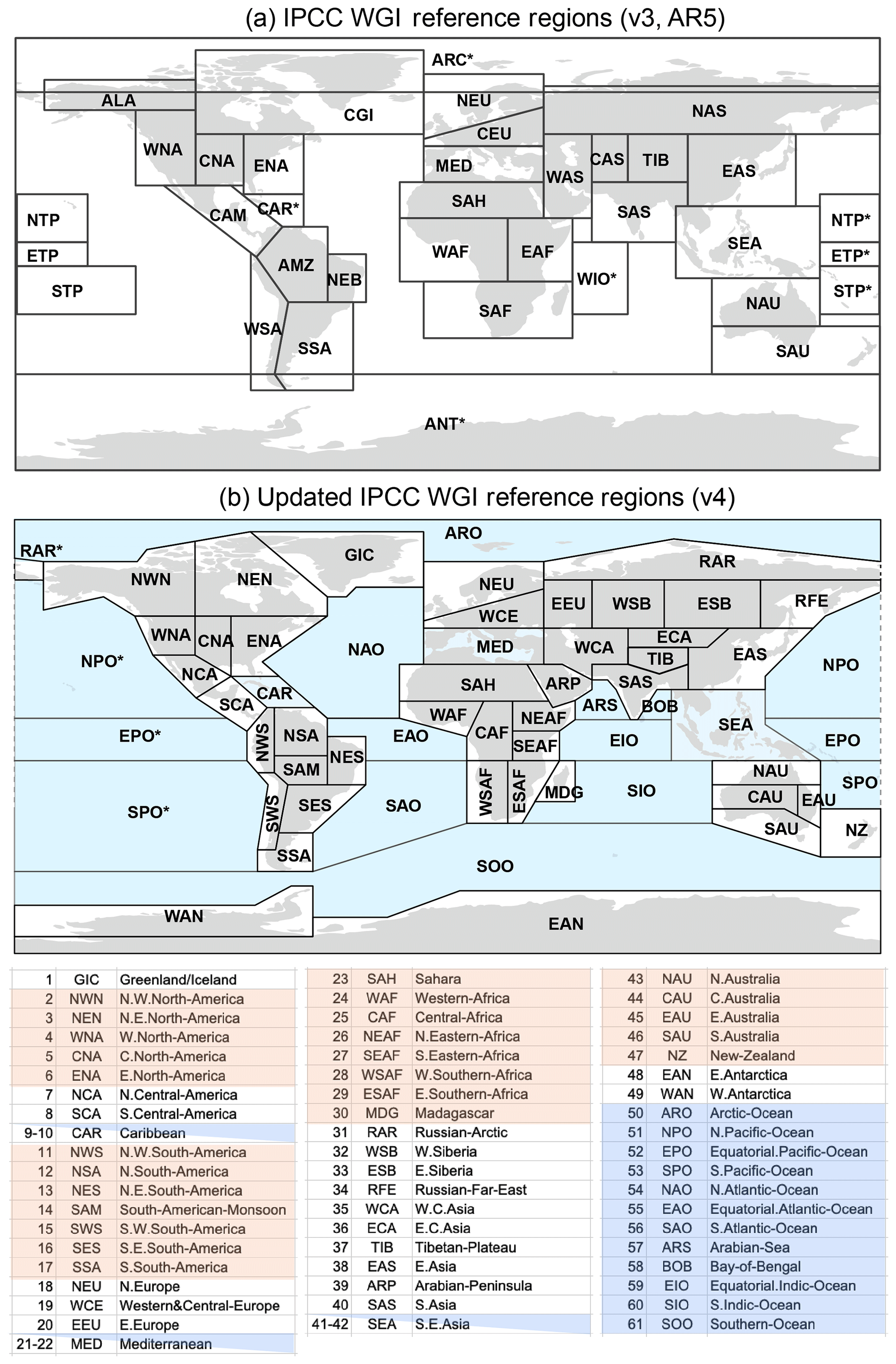
Figure 1Updated IPCC reference land (grey shading) and ocean (blue shading) regions; note that the Caribbean, SEA and the Mediterranean are considered both land and ocean regions (defined using the land and sea masks, respectively). Land masks are used to obtain land-only information for land regions (excluding the coastal white regions).
The increasing availability of CMIP6 multi-model simulations (O'Neill et al., 2016; NCC editorial, 2019) offers an opportunity to refine the AR5 reference regions – due to the higher atmospheric model resolution, typically around 1∘ – and also to produce ready-to-use aggregated regional information for the updated reference regions. This is a timely task due to the great interest of the research community in the higher sensitivity of some CMIP6 models and the potential implications for climate change studies (Forster et al., 2020). Here, we present the results of an initiative carried out during the last year to achieve this goal. First, we present the updated regions (referred to as IPCC WGI reference regions, version 4) and describe the rationale for the revision, which was guided by two basic principles: (1) climatic consistency and better representation of regional climate features and (2) representativeness of model results (sufficient number of model grid boxes per region). Climatic homogeneity is characterized in terms of mean temperature and precipitation considering Köppen–Geiger climatic regions (Rubel and Kottek, 2010), the annual cycle and projected changes over the reference regions. The resulting 46 land plus 15 ocean regions (see Fig. 1b) are provided as coordinates (in CSV format) and also as a shapefile with companion notebooks to illustrate their use in R and Python.
Second, we describe the monthly regional temperature and precipitation dataset obtained by spatially aggregating the model data over the reference regions (currently for CMIP5 and CMIP6, to be extended later to observations and additional datasets). Finally, the use of these reference regions, datasets and code is illustrated through a reproducible example which analyses the likely range of future temperature and precipitation changes that are expected for different European regions using scatter plots.
Section 2 presents the data and methods used in this work. Section 3 describes the reference regions and their rationale. The regionally aggregated CMIP5 dataset is presented in Sect. 4, and links are provided for additional aggregated datasets (e.g. CMIP6), which are periodically updated; a reproducible illustrative example is described in Sect. 5. Data and code availability are described in Sect. 6. Finally, conclusions and a discussion are presented in Sect. 7.
We use global gridded observations to characterize the regional climatological conditions at a subcontinental scale. In particular, we use CRU TS (version 4.03; Harris et al., 2014; Harris and Jones, 2020) providing monthly precipitation and temperature with a resolution of 0.5∘ over land for the period 1901–2017. Figure 2a–b show the annual mean temperature and precipitation climatology for the period 1981–2010. CRU TS does not cover Antarctica, which is therefore infilled with an alternative dataset, namely the EWEMBI gridded observations (Lange, 2019). Figure 2c shows the Köppen–Geiger climatic regions (Rubel and Kottek, 2010) computed from these datasets. Quantifying the observational uncertainty is an increasing concern in climate studies, particularly for precipitation (Kotlarski et al., 2019). Therefore, we use two additional observational datasets for precipitation in some parts of this study: (1) Global Precipitation Climatology Centre (GPCC, v2018; Schneider et al., 2011), providing monthly land precipitation values with 0.5∘ resolution for the period from 1891 to 2016, and (2) Global Precipitation Climatology Project (GPCP; monthly version 2.3 gridded, merged satellite–gauge precipitation; Huffman et al., 2009), providing monthly land and ocean precipitation values with a resolution of 2.5∘ for the period 1979–2018. We show results for the current WMO climatological standard normal period 1981–2010 (WMO, 2017).

Figure 2(a) Global mean temperature, (b) accumulated precipitation and (c) Köppen–Geiger climate classification from the CRU-TS dataset for the period 1981–2010 (data for Antarctica are filled with the EWEMBI dataset). This information is used to characterize the regional climate consistency of the reference regions (solid lines). (d, e) Climate change projections for temperature and precipitation, respectively, from the CMIP5 curated dataset for RCP8.5 2081–2100 w.r.t. the AR5 modern climate baseline 1986–2005. Hatching indicates weak (less than 80 %) model agreement on the sign of the change.
Global model scenario data were downloaded for CMIP5 (Taylor et al., 2012) and CMIP6 (O'Neill et al., 2016) models for the historical (1850–2005 and 1850–2014) and RCP2.6 and SSP1-2.6, RCP4.5 and SSP2-4.5, and RCP8.5 and SSP5-8.5 future scenarios (2006–2100 and 2015–2100). Data for CMIP5 (curated version used for IPCC-AR5) were downloaded from the IPCC Data Distribution Centre (DDC; https://www.ipcc-data.org/sim/gcm_monthly/AR5/index.html, last access: 31 December 2019) and for CMIP6 were downloaded from the Earth System Grid Federation (ESGF; Balaji et al., 2018); a periodically updated inventory is available at the ATLAS GitHub repository (in the AtlasHub-inventory folder). All model data have been interpolated to common 2∘ (for CMIP5) and 1∘ (CMIP6) grids – separately for land and ocean grid boxes using conservative remapping (using CDO with the models and target land–sea masks; CDO, 2019) – which are typical model resolutions for CMIP5 and CMIP6 models, respectively. The common grids and land–sea masks are available in the ATLAS GitHub repository (in the reference-grids folder).
In this paper we illustrate the results using the curated CMIP5 dataset and refer to the ATLAS GitHub repository for similar results for CMIP6. Figure 2d–e show the CMIP5 multi-model climate change signal for annual mean temperature (in absolute terms) and precipitation (relative, in per cent) for RCP8.5 2081–2100 (with respect to the modern climate baseline 1986–2005 used in AR5). This figure shows the typical spatial climate change patterns and is used to illustrate the consistency of the regional signals in the climate reference regions.
The Giorgi reference regions were originally defined with the goal to represent consistent climatic regimes and physiographic settings while maintaining an appropriate size for model representation (thousands of kilometres, to contain several model grid boxes), using some subjectivity in the final selection (Giorgi and Francisco, 2000). Here, we are guided by the same basic principles to define a new version of the reference regions (see Fig. 1b). Climatic homogeneity is characterized in terms of mean temperature and precipitation considering Köppen–Geiger climatic regions (see Fig. 2) and also the annual precipitation cycle (Figs. 3 and 4); in the latter case, observational uncertainty is analysed using the three alternative datasets described in Sect. 2. Representativity of model results (sufficient number of grid boxes per region) is analysed at the end of this section in Fig. 5.
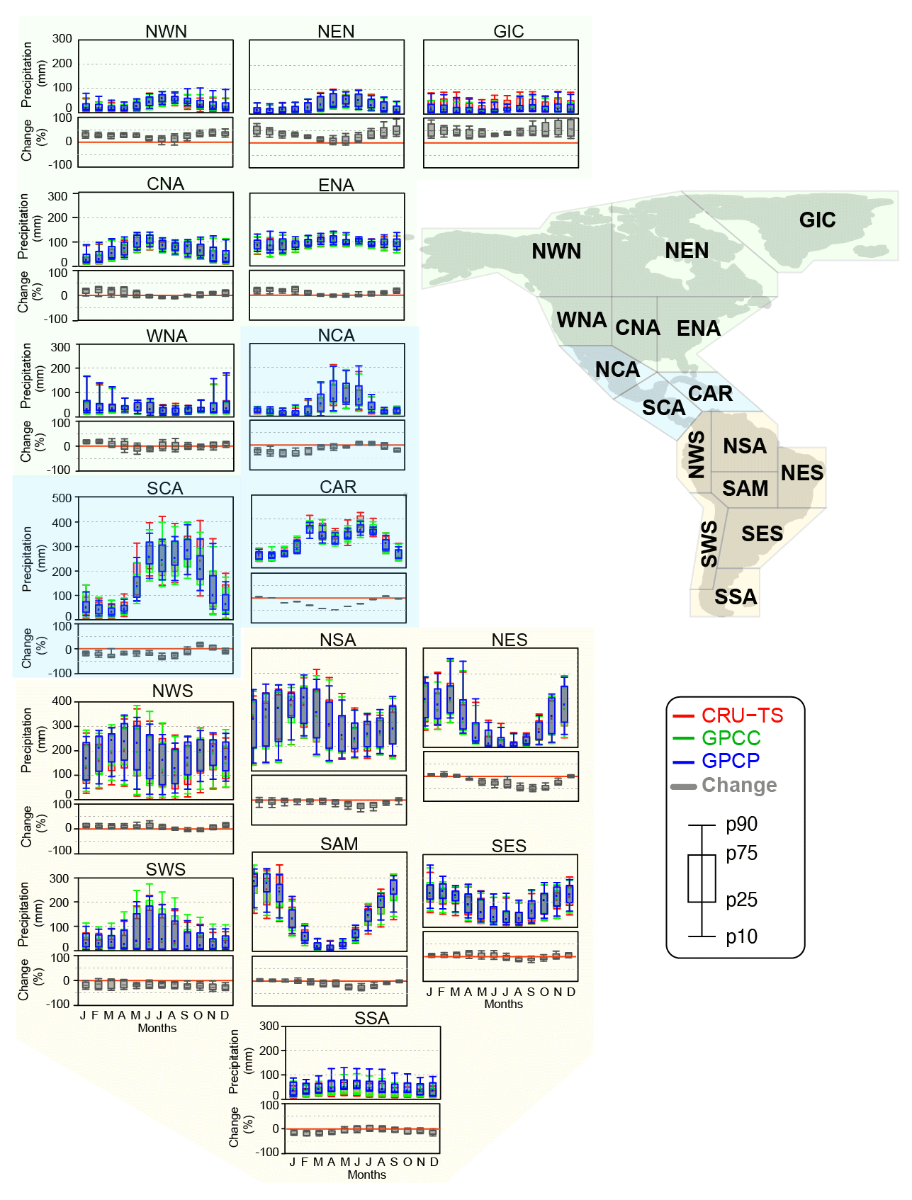
Figure 3Observed annual cycle (1981–2010) for precipitation for the American reference regions from three different observational datasets (CRU-TS, GPCC, GPCP) and climate change signal (RCP8.5, 2081–2100, w.r.t. the AR5 modern climate baseline 1986–2005). The panel for each reference region shows the observed annual cycle (top, in monthly accumulated millimetres) and the monthly projected changes (bottom, in grey, as percentages); box-and-whisker plots represent the spatial (grid box) spread of monthly values over the region.
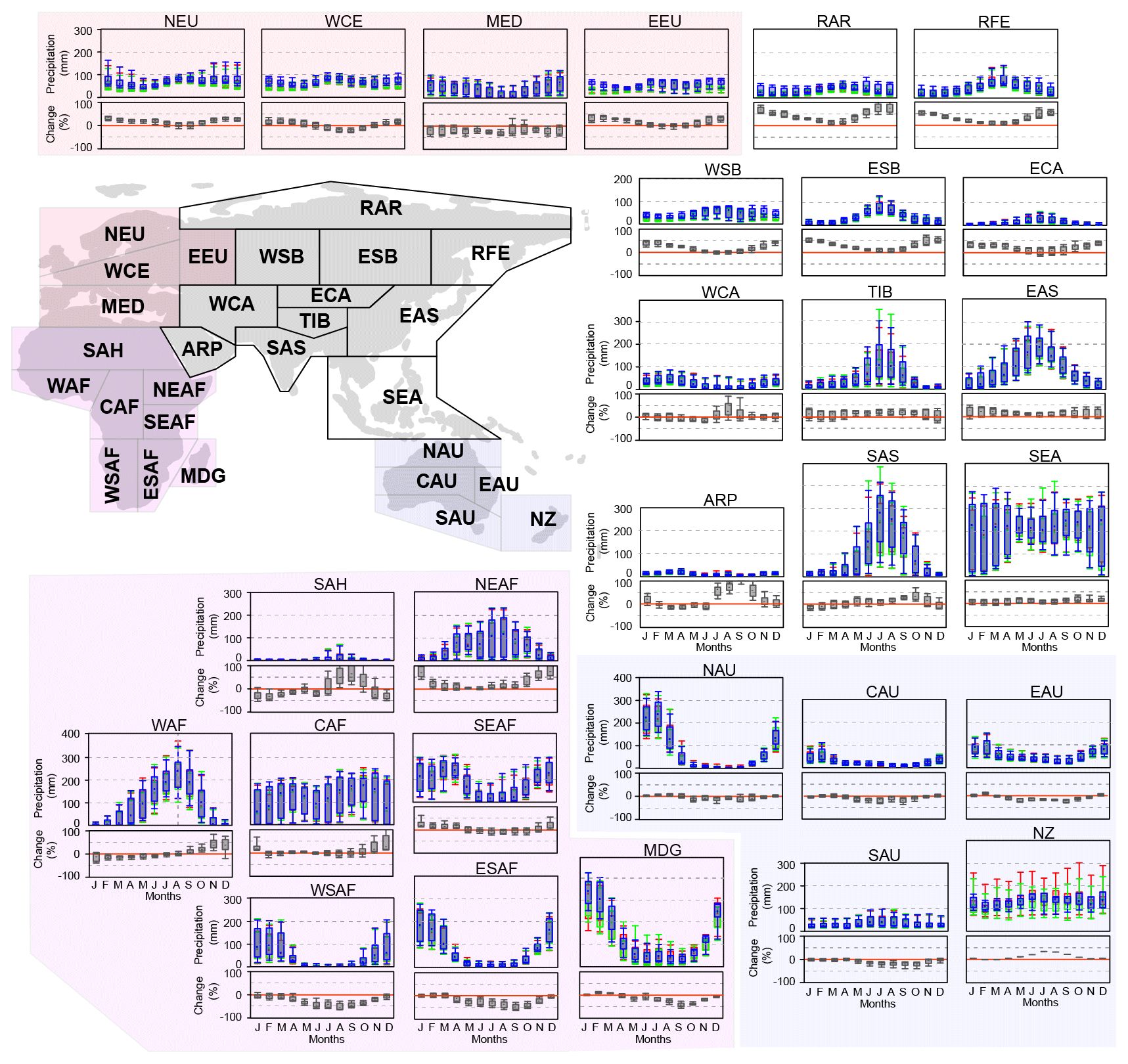
Figure 4As in Fig. 3 but for Europe, Asia and Australasia.
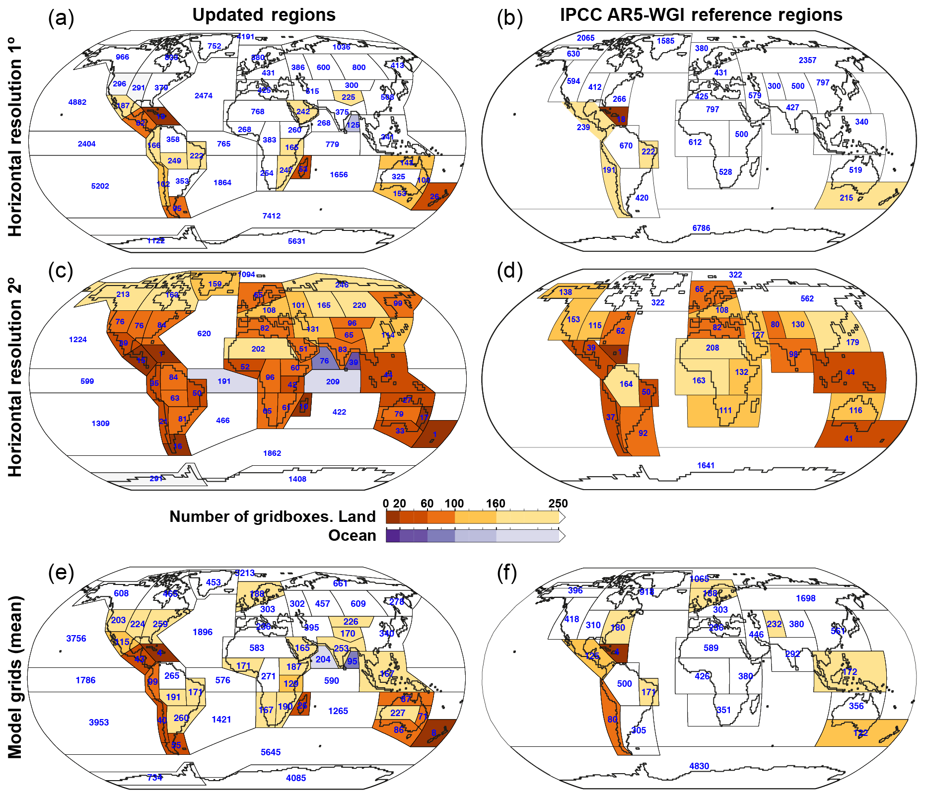
Figure 5Number of grid boxes encompassed by the different reference regions for 1∘ (a, b) and 2∘ (c, d) resolution and for the CMIP6 model grids (e, f) – the multi-model mean is represented – considering the updated (a, c, e) and the original AR5 (b, d, f) reference regions. Colours indicate regions with fewer than 250 grid boxes. The blue numbers in each of the regions show the number of grid boxes (only land grid boxes for land regions).
3.1 Definition of new regions
Here we describe the rationale for the new version of the reference regions presented in this paper (version 4; see Fig. 1b) which is based on the latest available version (version 3; see Fig. 1a) that was used in AR5. In contrast to the AR5 regions, the new version includes 16 oceanic regions suitable for the analysis of large-scale atmospheric data. Many of the new land regions are defined by splitting the previous ones to increase climatic homogeneity as described below.
In North America, the AR5 polar Greenland–Iceland (GIC) region is divided in two, northeastern North America (NEN) and Greenland–Iceland (GIC), to better accommodate the subarctic and polar climates, respectively (Fig. 2c). The eastern and central North American regions (ENA and CNA) are maintained mostly unaltered while the western part is reorganized to increase climate consistency. The new northwestern region (NWN) includes mostly the subarctic regions, whereas the modified western region (WNA) encompasses a variety of regional intermixed climates (semiarid, Mediterranean and continental; see Fig. 2c) which are difficult to further separate due to the complex orography.
The new north Central America (NCA) region includes the semiarid and arid climates of northern Mexico, separating them from the tropical climates in southern Central America which constitute a new region (SCA). The Caribbean (CAR) region has been modified to fully include the Greater Antilles.
In South America, the AR5 northwestern Amazonia region is divided into three subregions to separate the northern South America (NSA) region from the western region (NWS) – which includes the northern Andes mountain range – and the South America monsoon (SAM) region. These regions represent subcontinental areas of greater climatic coherency (Espinoza et al., 2019), in terms of both climate and climate change signals (Fig. 2c–e), and exhibit characteristic seasonal precipitation cycles (Fig. 3), with a rainy season from October to March in SAM and no clear wet and dry seasons for NSA and NWS. The northeastern region is maintained, but the name is changed to northeastern South America (NES). The old southern South America region is divided in two, separating the northern (southeastern South America, SES) and southern (SSA) parts, the later encompassing the mostly cold desert climates exhibited in this region (see Fig. 2c).
The three European reference regions NEU, CEU (renamed western and central Europe, WCE) and MED have been maintained unaltered since they encompass the main regional climates in Europe, from subarctic to oceanic–continental to Mediterranean. However, an additional region has been introduced in eastern Europe (EEU), encompassing the continental climate on the western side of the Urals mountain range.
For Africa, the AR5 WAF region has been divided in two (WAF and CAF); although these regions have similar Köppen–Geiger climates (see Fig. 2c), they have very different annual cycles (Fig. 4) and therefore should be analysed independently (Diedhiou et al., 2018). A similar situation was found in the original EAF (Osima et al., 2018) which was also divided in two: a northern subregion (NEAF), which includes the arid region of the Horn of Africa, and a southern subregion (SEAF). These two regions also exhibit different precipitation seasonal cycles, with different timing of the annual maximum (see Fig. 4). Moreover, the South Africa region SAF was also divided into subregions with different rainfall regimes (Maúre et al., 2018): the western subregion (WSAF), including the arid regional climates, and the eastern region (ESAF). Additionally, the (sub)tropical region of Madagascar (MDG) was split from the continent.
In the case of Asia, northern Asia is subdivided into a northern subarctic region (RAR), two regions for Western (WSB) and Eastern (ESB) Siberia, and a region for the Russian Far East (RFE). The original western Asia region (WAS) is divided into two regions: western central Asia (WCA) and the Arabian Peninsula (ARP), the latter with an arid climate; these two subregions exhibit a distinct seasonal cycle (see Fig. 4). The old Tibetan Plateau (TIB) region is divided into two subregions, separating the highland climate of the Tibetan Plateau in the south (TIB) from the northern arid subregion (eastern central Asia, ECA). The South Asia (SAS), East Asia (EAS) and Southeast Asia (SEA) regions are maintained unaltered, with the exception of adjustments caused by changes in neighbouring regions and the definition of two ocean regions (the Arabian Sea and the Bay of Bengal) for the oceanic part of the original SAS.
Regarding Australasia, the southern region (SAU) is now further south, better differentiating the rainfall climatology (Fig. 2c) and separated from the oceanic New Zealand (NZ). The northern region is divided into three subregions to increase climatic consistency (CSIRO and Bureau of Meteorology, 2015; see Fig. 1b), separating the northern tropical region (NAU), the central arid region (CAU) and the subtropical east coast (EAU).
In contrast to the version 3 reference regions used in AR5, those defined in this paper also include 15 oceanic regions (note that the Caribbean, the Mediterranean and Southeast Asia are considered both land and ocean regions, defined using the land and sea masks, respectively). In version 3 only selected sub-domains of the Indian and tropical Pacific Ocean were designated as reference regions and the rest of the main oceanic regions were not represented. Version 4 includes representation of all major oceanic regions. The equatorial and northern and southern extents of each of the main non-polar oceans are defined as separate regions with the added refinement of dividing the “northern Indian ocean” in two: the Arabian Sea and the Bay of Bengal. The Arctic Ocean is defined as the region north of the main Eurasian and North American landmass which then also defines the northern extent of the North Pacific and Atlantic regions. The equatorial regions extend from 10∘ S to 10∘ N to include those regions used to define indices for both El Niño and the Indian Ocean Dipole. The southern extents of the South Pacific, Atlantic and Indian regions are similar to those defined by Durack and Wijffels (2010), with the remaining ocean region to the south defined as a single Southern Ocean region.
Since these ocean regions largely exclude the coastal zones (which are often included in the land regions), they are generally more suitable for the analysis of large-scale atmospheric data. Figure 2d and e demonstrate that in this respect the ocean regions are a good addition to the AR5 definitions even though they were not developed with the intention of defining ocean basin masks for zonal means used by oceanographers. However, we note that since the coastal regions can be defined by applying a land–sea mask to the land boxes, it is possible to combine regions to enable the more traditional ocean basin definitions used by oceanographers to be produced to a large extent (albeit not exactly).
3.2 Representativeness of model results
The higher atmospheric resolution of CMIP6 yields better model representation on the reference regions (more grid boxes per region) allowing a revision for better climatic consistency (e.g. dividing heterogeneous regions) while preserving model representativeness. Figure 5 illustrates this, displaying the number of grid boxes (only land grid boxes for land regions) in each of the AR5 (last column) and revised (first column) reference regions for the two reference grids (1 and 2∘), as well as for the CMIP6 model grids (representing the multi-model mean of grid box numbers). This figure shows that the 1∘ grid provides a good reference for CMIP6. Moreover, it shows that the new reference regions are more representative than the AR5 ones due to the increase in model resolution (see Fig. 5a and d, corresponding to the cases of CMIP6 data on the updated reference regions and to CMIP5 data in the original AR5 regions, respectively). The regions with the smallest number of grid boxes correspond to three island regions: the Caribbean (CAR), New Zealand (NZ) and Madagascar (MDG), with around 20–60 grid boxes per region. Note that the updated regions are also suitable for the analysis of CMIP5 data (at 2∘ resolution; Fig. 5c) since all regions encompass over 10 land grid boxes, with the exception of the three above-mentioned regions, where results should be interpreted with caution.
These updated regions are defined as polygons (the lines in Fig. 1 are straight lines on a projected plane) and are provided as coordinates and a shapefile at the ATLAS GitHub (reference-regions folder); the reference grids and land–sea masks can be found in the reference-grids folder. Moreover, companion R and Python notebooks are also available (reference-regions/notebooks) to illustrate their use in practical problems (e.g. calculating regional averages).
The seasonal mean temperature and precipitation in CMIP5 models averaged over the version 3 (AR5) reference regions comprise a popular dataset, suitable for the regional analysis of climate projections and their uncertainties (McSweeney et al., 2015). Here we extend this idea to the new regions and model data and compute aggregated monthly results over the different reference regions (see Fig. 1b) for all the CMIP5 simulations (and also the available CMIP6 ones), considering land-only, sea-only and land–sea grid boxes (the land–sea masks are available in the ATLAS GitHub repository, reference-grids). Results are calculated for each model simulation and stored individually as a text CSV file, with regions in columns (including the global results in the last column) and dates (months) in rows; results for one ensemble member per model are included directly in the ATLAS GitHub repository (aggregated-datasets folder), and links are provided to the general dataset (full ensemble with all runs) which allows for internal variability studies.
Whereas the aggregated CMIP5 dataset is final, results for CMIP6 will be regularly updated when new data become available at the ESGF; these two datasets constitute alternative lines of evidence for climate change studies, and the ATLAS initiative presented here facilitates intercomparison of results and consistency checks for the reference climatic regions. Note that although the aggregated data provide summary climate information for each subcontinental region which is useful for a broad spectrum of users, detailed climate information at local or regional scales (in each subcontinental region) would be required for further regional analysis.
To demonstrate a potential application of the reference regions and the associated regionally averaged CMIP data (for temperature and precipitation), we show a simple case study illustrating the projected range of future temperature and precipitation change. This can provide useful context information for a variety of impact and adaptation studies. In particular, we use scatter plots to show the median and 10th and 90th percentiles of the CMIP5 ensemble change. We focus on three illustrative European regions (NEU, WCE and MED) with opposite climate change signals for precipitation (see Fig. 2e). The code and data needed to run this example (which can be extended to other regions, or combination of regions, and datasets, e.g. CMIP6) are all available at the ATLAS GitHub repository (aggregated-datasets/scripts folder) and can be run in a local R session accessing the GitHub data with no further requirements.
Figure 6 shows the projected changes in annual mean temperature and precipitation resulting from the script scatterplots_TvsP.R. In particular, results from RCP2.6, RCP4.5 and RCP8.5 scenarios for the early (2021–2040), middle (2041–2060 and 2061–2080) and late (2081–2100) 21st century – relative to the 1986–2005 baseline period – for each of the three European subregions are displayed. This figure projects an increase in temperature in all European domains – with similar warming in all regions for the different scenarios and future periods – and a consistent meridional gradient of changes in precipitation, with a clear precipitation increase in NEU, non-changing conditions in WCE (uncertainty range crossing the zero line) and reduced precipitation over MED. The same scripts can be applied to the currently available CMIP6 dataset by changing two parameters to check the consistency of these results for the updated models and scenarios.
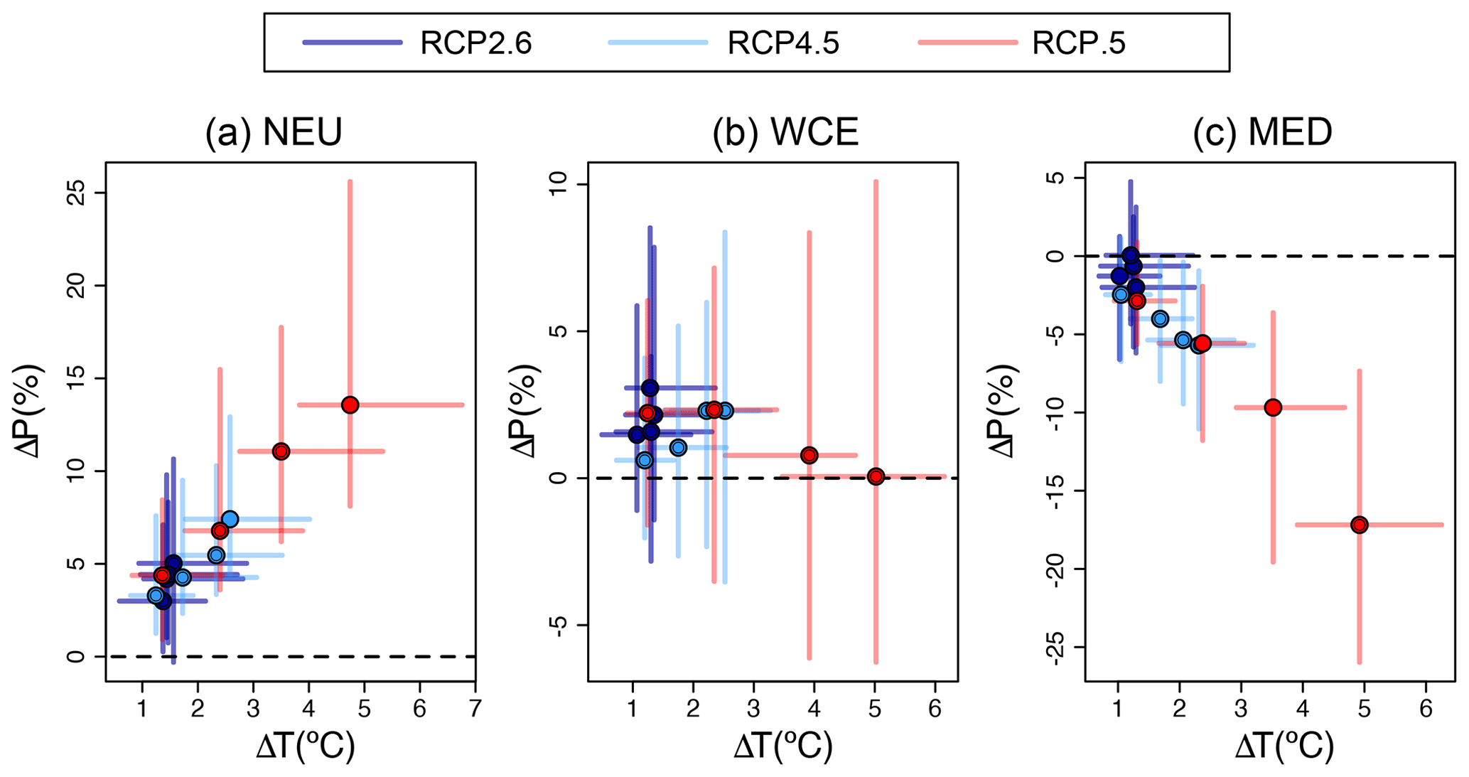
Figure 6Illustrative example of the use of reference regions and aggregated CMIP5 datasets: regional mean changes in annual mean temperature and precipitation for three European regions (NEU, WCE and MED) for four future periods (2021–2040, 2041–2060, 2061–2080, 2081–2100), as obtained from CMIP5 projections. Changes are absolute for temperature and relative for precipitation. Horizontal and vertical error bars represent ±1 standard deviation from the mean calculated across the ensemble of included models. The script to generate this figure for all the 61 land and ocean regions (as well as the global results) from the aggregated and ready-to-use CMIP5 datasets is available at the ATLAS GitHub and can be adapted to produce similar results for alternative datasets (e.g. CMIP6).
Note that this illustrative example can be modified to serve different purposes. For instance, the same diagram can be adapted to display the individual model values (or to select the subset of models spanning the uncertainty range) in order to assist in the comparison and the selection of representative sub-ensembles for impact studies (e.g. Ruane and McDermid, 2017). The calculation of the regional aggregated values is time-consuming (computed offline and results are provided in the GitHub repository); however, accessing the values and plotting the results is straightforward and the scripts provided run in a few seconds.
The present work is part of the climate change ATLAS initiative (which is aligned with IPCC AR6 activities). The definitions of the regions, the code and the spatially aggregated datasets are available at the GitHub ATLAS repository: https://github.com/SantanderMetGroup/ATLAS, https://doi.org/10.5281/zenodo.3998463 (Iturbide et al., 2020). The regions and CMIP5 aggregated data are distributed under the Creative Commons Attribution (CC-BY) 4.0 licence, whereas the scripts and code are made available under the GNU General Public License (GPL) v3.0. The ATLAS project builds on the publicly available climate4R R framework (Iturbide et al., 2019; available under the GNU General Public License v3.0) and provides additional functions which may be relevant for the users of the reference regions and aggregated datasets, such as the calculation of global warming levels, thus enhancing the functionalities presented in this work. The Python notebook is based on the regionmask (Hauser, 2020) and xarray (Hoyer and Hamman, 2017) packages, among others. The results for CMIP5 are based on the final curated dataset used for IPCC-AR5, but other datasets will be updated periodically when new data become available (e.g. CMIP6, still in progress).
Regarding the original datasets used in this work, all of them are publicly available from the local providers – CRU TS4.03 is distributed under the Open Database License and EWEMBI and GPCC v2018 are distributed under a Creative Commons Attribution 4.0 International licence – and/or the Earth System Grid Federation (ESGF; Balaji et al., 2018) – CMIP5 and CMIP6. Moreover, for the sake of reproducibility some datasets have also been replicated at the Santander Climate Data Service which is transparently accessible from climate4R via the User Data Gateway (registration is required to accept the terms of use of the original datasets; more information at http://meteo.unican.es/udg-wiki, last access: 30 July 2020).
A new set of 46 land plus 15 ocean regions is introduced in this work updating the previous version of IPCC AR5-WGI reference regions for the regional synthesis of observed and simulated climate change datasets (in particular for the new CMIP6 simulations). The new regions increase the climatic consistency of the previous ones – by rearranging and dividing regions exhibiting mixed regional climates – and have a suitable model representation (the minimum is in the range 20–60 model grid boxes for three particular island regions: the Caribbean, New Zealand and Madagascar). This revision was guided by the basic principles of climatic consistency and model representativeness, but there is of course some subjectivity in the final selection.
We also present a new dataset of monthly spatially aggregated information using the new reference regions and the available CMIP5 data (from the IPCC DDC) and CMIP6 data (from the ESGF, as of 30 September 2019) and describe a worked example of how to use this dataset to inform regional climate change studies, in particular about the likely range of future temperature and precipitation changes for the different European reference regions using scatter plots.
JMG and MI conceived the study and wrote the code and the manuscript; BvdH conceived the case study; MI and MH implemented the R and Python companion notebooks; all authors contributed to the definition of the regions and to the discussion and revised the text and the results.
The authors declare that they have no conflict of interest.
We acknowledge the World Climate Research Programme's Working Group on Coupled Modelling, which is responsible for CMIP, and we thank the climate modelling groups (listed in the ATLAS GitHub) for producing and making available their model output. The authors are also grateful to the two reviewers (Chris Brierley and one anonymous), who helped to improve the original manuscript with detailed in-depth revision providing constructive comments, and to Michael Grose and Jason Evans, who provided useful comments during the interactive discussion.
This research has been supported by the Spanish National Plan for Scientific and Technical Research and Innovation (project PID2019-111481RB-I00 and María de Maeztu excellence programme projects MdM-2017-0765 and MdM-2017-0714), FCT MCTES financial support to CESAM (UIDP/50017/2020+UIDB/50017/2020), and the Basque Government BERC 2018–2021 programme.
This paper was edited by David Carlson and reviewed by Chris Brierley and one anonymous referee.
Balaji, V., Taylor, K. E., Juckes, M., Lawrence, B. N., Durack, P. J., Lautenschlager, M., Blanton, C., Cinquini, L., Denvil, S., Elkington, M., Guglielmo, F., Guilyardi, E., Hassell, D., Kharin, S., Kindermann, S., Nikonov, S., Radhakrishnan, A., Stockhause, M., Weigel, T., and Williams, D.: Requirements for a global data infrastructure in support of CMIP6, Geosci. Model Dev., 11, 3659–3680, https://doi.org/10.5194/gmd-11-3659-2018, 2018.
Bärring, L. and Strandberg, G.: Does the projected pathway to global warming targets matter?, Environ. Res. Lett., 13, 024–029, https://doi.org/10.1088/1748-9326/aa9f72, 2018.
CDO: Climate Data Operator Version 1.9.8. Max-Planck-Institute for Meteorology, available at: https://code.mpimet.mpg.de/projects/cdo (last access: 30 July 2020), 2019.
Christensen, J., Hewitson, B., Busuioc, A., Chen, A., Gao, X., Held, I., Jones, R., Kolli, R., Kwon, W.-T., Laprise, R., Rueda, V. M., Mearns, L., Menez, C., Rn, J., Rinke, A., Sarr, A., and Whetton, P.: Climate Change 2007: The Physical Science Basis. Contribution of Working Group I to the Fourth Assessment Report of the Intergovernmental Panel on Climate Change, edited by: Solomon, S., Qin, D., Manning, M., Chen, Z., Marquis, M., Averyt, K. B., Tignor, M., and Miller, H. L., Regional Climate Projections, 847–940, Cambridge University Press, Cambridge, United Kingdom and New York, NY, USA, 2007.
CSIRO and Bureau of Meteorology: Climate Change in Australia Information for Australia's Natural Resource Management Regions: Technical Report, CSIRO and Bureau of Meteorology, Australia, available at: http://www.climatechangeinaustralia.gov.au (last access: 30 July 2020), 2015.
Diedhiou, A., Bichet, A., Wartenburger, R., Seneviratne, S. I., Rowell, D. P., Sylla, M. B., Diallo, I., Todzo, S., Touré, N. E., Camara, M., Ngatchah, B. N., Kane, N. A., Tall, L., and Affholder, F.: Changes in climate extremes over West and Central Africa at 1.5 ∘C and 2 ∘C global warming, Environ. Res. Lett., 13, 065020, https://doi.org/10.1088/1748-9326/aac3e5, 2018.
Durack, P. J. and Wijffels, S. E.: Fifty-Year Trends in Global Ocean Salinities and Their Relationship to Broad-Scale Warming, J. Climate, 23, 4342–4362, https://doi.org/10.1175/2010JCLI3377.1, 2010.
Espinoza, J. C., Ronchail, J., Marengo, J. A., and Segura, H.: Contrasting North–South changes in Amazon wet-day and dry-day frequency and related atmospheric features (1981–2017), Clim. Dynam., 52, 5413–5430, https://doi.org/10.1007/s00382-018-4462-2, 2019.
Forster, P. M., Maycock, A. C., McKenna, C. M., and Smith, C. J.: Latest climate models confirm need for urgent mitigation, Nat. Clim. Change, 10, 7–10, https://doi.org/10.1038/s41558-019-0660-0, 2020.
Giorgi, F. and Francisco, R.: Uncertainties in regional climate change prediction: a regional analysis of ensemble simulations with the HADCM2 coupled AOGCM, Clim. Dynam., 16, 169–182, https://doi.org/10.1007/PL00013733, 2000.
Giorgi, F., Hewitson, B., Christensen, J., Hulme, M., Storch, H. V., Whetton, P., Jones, R., Mearns, L., and Fu, C.: Climate Change 2001: The Scientific Basis, edited by: Houghton, J. T., Ding, Y., Griggs, D. J., Noguer, M., vad der Linden, P. J., Dai, X., Maskell, K., and Johnson, C. A., Regional Climate Information, Evaluation and Projections, 583–638, Cambridge University Press, Cambridge, United Kingdom and New York, NY, USA, 2001.
Harris, I. and Jones, P.: CRU TS4.03: Climatic Research Unit (CRU) Time-Series (TS) version 4.03 of high-resolution gridded data of month-by-month variation in climate (Jan. 1901–Dec. 2018), Centre for Environmental Data Analysis, https://doi.org/10.5285/10d3e3640f004c578403419aac167d82, 2020.
Harris, I., Jones, P. D., Osborn, T. J., and Lister, D. H.: Updated high-resolution grids of monthly climatic observations – the CRU TS3.10 Dataset, Int. J. Climatol., 34, 623–642, https://doi.org/10.1002/joc.3711, 2014.
Hauser, M.: Regionmask: plotting and creation of masks of spatial regions (Version 0.6.1), Zenodo, https://zenodo.org/record/3992368#.X5-UPzEo-yV, last access: 13 November 2020.
Hawkins, E. and Sutton, R.: The Potential to Narrow Uncertainty in Regional Climate Predictions, B. Am. Meteorol. Soc., 90, 1095–1108, https://doi.org/10.1175/2009BAMS2607.1, 2009.
Hoyer, S. and Hamman, J.: xarray: N-D labeled Arrays and Datasets in Python, Journal of Open Research Software, 5, 10, https://doi.org/10.5334/jors.148, 2017.
Huffman, G. J., Adler, R. F., Bolvin, D. T., and Gu, G.: Improving the global precipitation record: GPCP Version 2.1, Geophys. Res. Lett., 36, L17808, https://doi.org/10.1029/2009GL040000, 2009.
Iturbide, M., Bedia, J., Herrera, S., Baño-Medina, J., Fernández, J., Frías, M. D., Manzanas, R., San-Martín, D., Cimadevilla, E., Cofiño, A. S., and Gutiérrez, J. M.: The R-based climate4R open framework for reproducible climate data access and post-processing, Environ. Modell. Softw., 111, 42–54, https://doi.org/10.1016/j.envsoft.2018.09.009, 2019.
Iturbide, M., Gutiérrez, J. M., Cimadevilla, E., Bedia, J., Hauser, M., and Manzanas, R.: SantanderMetGroup/ATLAS GitHub (Version v1.6), Zenodo, https://doi.org/10.5281/zenodo.3998463, 2020.
Kotlarski, S., Szabó, P., Herrera, S., Räty, O., Keuler, K., Soares, P. M., Cardoso, R. M., Bosshard, T., Pagé, C., Boberg, F., Gutiérrez, J. M., Isotta, F. A., Jaczewski, A., Kreienkamp, F., Liniger, M. A., Lussana, C., and Pianko-Kluczyńska, K.: Observational uncertainty and regional climate model evaluation: A pan-European perspective, Int. J. Climatol., 39, 3730–3749, https://doi.org/10.1002/joc.5249, 2019.
Lange, S.: EartH2Observe, WFDEI and ERA-Interim data Merged and Bias-corrected for ISIMIP (EWEMBI), V. 1.1, GFZ Data Services, https://doi.org/10.5880/pik.2019.004, 2019.
Madakumbura, G. D., Kim, H., Utsumi, N., Shiogama, H., Fischer, E. M., Seland, A., Scinocca, J. F., Mitchell, D. M., Hirabayashi, Y., and Oki, T.: Event-to-event intensification of the hydrologic cycle from 1.5 ∘C to a 2 ∘C warmer world, Sci. Rep.-UK, 9, 1–7, https://doi.org/10.1038/s41598-019-39936-2, 2019.
Maúre, G., Pinto, I., Ndebele-Murisa, M., Muthige, M., Lennard, C., Nikulin, G., Dosio, A., and Meque, A.: The southern African climate under 1.5 ∘C and 2 ∘C of global warming as simulated by CORDEX regional climate models, Environ. Res. Lett., 13, 065002, https://doi.org/10.1088/1748-9326/aab190, 2018.
McSweeney, C. F., Jones, R. G., Lee, R. W., and Rowell, D. P.: Selecting CMIP5 GCMs for downscaling over multiple regions, Clim. Dynam., 44, 3237–3260, https://doi.org/10.1007/s00382-014-2418-8, 2015.
NCC editorial: The CMIP6 landscape, Nat. Clim. Change, 9, 727–727, https://doi.org/10.1038/s41558-019-0599-1, 2019.
O'Neill, B. C., Tebaldi, C., van Vuuren, D. P., Eyring, V., Friedlingstein, P., Hurtt, G., Knutti, R., Kriegler, E., Lamarque, J.-F., Lowe, J., Meehl, G. A., Moss, R., Riahi, K., and Sanderson, B. M.: The Scenario Model Intercomparison Project (ScenarioMIP) for CMIP6, Geosci. Model Dev., 9, 3461–3482, https://doi.org/10.5194/gmd-9-3461-2016, 2016.
Osima, S., Indasi, V. S., Zaroug, M., Endris, H. S., Gudoshava, M., Misiani, H. O., Nimusiima, A., Anyah, R. O., Otieno, G., Ogwang, B. A., Jain, S., Kondowe, A. L., Mwangi, E., Lennard, C., Nikulin, G., and Dosio, A.: Projected climate over the Greater Horn of Africa under 1.5 ∘C and 2 ∘C global warming, Environ. Res. Lett., 13, 065004, https://doi.org/10.1088/1748-9326/aaba1b, 2018.
Ruane, A. C. and McDermid, S. P.: Selection of a representative subset of global climate models that captures the profile of regional changes for integrated climate impacts assessment, Earth Perspectives, 4, 1, https://doi.org/10.1186/s40322-017-0036-4, 2017.
Rubel, F. and Kottek, M.: Observed and projected climate shifts 1901–2100 depicted by world maps of the Köppen-Geiger climate classification, Meteorol. Z., 19, 135–141, https://doi.org/10.1127/0941-2948/2010/0430, 2010.
Schneider, U., Becker, A., Finger, P., Meyer-Christoffer, A., Rudolf, B., and Ziese, M.: GPCC Full Data Reanalysis Version 6.0 at 0.5: Monthly Land-Surface Precipitation from Rain-Gauges built on GTS-based and Historic Data, https://doi.org/10.5676/DWD_GPCC/FD_M_V7_050, 2011.
Seneviratne, S., Nicholls, N., Easterling, D., Goodess, C., Kanae, S., Kossin, J., Luo, Y., Marengo, J., McInnes, K., Rahimi, M., Reichstein, M., Sorteberg, A., Vera, C., and Zhang, X.: Managing the Risks of Extreme Events and Disasters to Advance Climate Change Adaptation, edited by: Field, C. B., Barros, V., Stocker, T. F., and Dahe, Q., Changes in climate extremes and their impacts on the natural physical environment, 109–230, Cambridge University Press, Cambridge, United Kingdom and New York, NY, USA, 2012.
Taylor, K. E., Stouffer, R. J., and Meehl, G. A.: An Overview of CMIP5 and the Experiment Design, B. Am. Meteorol. Soc., 93, 485–498, https://doi.org/10.1175/BAMS-D-11-00094.1, 2012.
van Oldenborgh, G. J., Collins, M., Arblaster, J., Christensen, J. H., Marotzke, J., Power, S. B., Rummukainen, M., and Zhou, T.: Climate Change 2013: The Physical Science Basis. Contribution of Working Group I to the Fifth Assessment Report of the Intergovernmental Panel on Climate Change, edited by: Stocker, T. F., Qin, D., Plattner, G.-K., Tignor, M., Allen, S. K., Boschung, J., Nauels, A., Xia, Y., Bex, V., and Midgley, P. M., Annex I: Atlas of Global and Regional Climate Projections, 1311–1394, https://doi.org/10.1017/CBO9781107415324.029, Cambridge University Press, Cambridge, United Kingdom and New York, NY, USA, 2013.
WMO: WMO Guidelines on the Calculation of Climate Normals, WMO – No. 1203, available at: https://library.wmo.int/doc_num.php?explnum_id=4166 (last access: 30 July 2020), 2017.