A long-term (2005–2016) dataset of hourly integrated land–atmosphere interaction observations on the Tibetan Plateau

The Tibetan Plateau (TP) plays a critical role in influencing regional and global climate, via both thermal and dynamical mechanisms. Meanwhile, as the largest high-elevation part of the cryosphere outside the polar regions, with vast areas of mountain glaciers, permafrost and seasonally frozen ground, the TP is characterized as an area sensitive to global climate change. However, meteorological stations are biased and sparsely distributed over the TP, owing to the harsh environmental conditions, high elevations, complex topography and heterogeneous surfaces. Moreover, due to the weak representation of the stations, atmospheric conditions and the local land–atmosphere coupled system over the TP as well as its effects on surrounding regions are poorly quantified. This paper presents a long-term (2005–2016) in situ observational dataset of hourly land–atmosphere interaction observations from an integrated high-elevation and cold-region observation network, composed of six field stations on the TP. These in situ observations contain both meteorological and micrometeorological measurements including gradient meteorology, surface radiation, eddy covariance (EC), soil temperature and soil water content profiles. Meteorological data were monitored by automatic weather stations (AWSs) or planetary boundary layer (PBL) observation systems. Multilayer soil temperature and moisture were recorded to capture vertical hydrothermal variations and the soil freeze–thaw process. In addition, an EC system consisting of an ultrasonic anemometer and an infrared gas analyzer was installed at each station to capture the high-frequency vertical exchanges of energy, momentum, water vapor and carbon dioxide within the atmospheric boundary layer. The release of these continuous and long-term datasets with hourly resolution represents a leap forward in scientific data sharing across the TP, and it has been partially used in the past to assist in understanding key land surface processes. This dataset is described here comprehensively for facilitating a broader multidisciplinary community by enabling the evaluation and development of existing or new remote sensing algorithms as well as geophysical models for climate research and forecasting. The whole datasets are freely available at the Science Data Bank (https://doi.org/10.11922/sciencedb.00103; Ma et al., 2020) and additionally at the National Tibetan Plateau Data Center (https://doi.org/10.11888/Meteoro.tpdc.270910, Ma 2020).

1 Introduction

The Tibetan Plateau (TP) is the world's highest and largest plateau, with highly complex terrain, and is referred to as the “Third Pole of the World” (Qiu, 2008). Moreover, the TP has the most extensive high-elevation distribution of cryosphere outside the polar regions. There are vast areas of mountain glaciers, snow, permafrost and seasonally frozen earth across the TP (Zhou and Guo, 1982; Kang et al., 2010; Cheng and Jin, 2013). Therefore, it also acts as the “Water Tower of Asia” (Immerzeel et al., 2010). Numerous research indicates that the TP plays an essential role in controlling regional and global climate through its thermal and mechanical mechanisms (Manabe and Broccoli, 1990; Yanai et al., 1992; Duan and Wu, 2005; Liu et al., 2007). It exerts major control on atmospheric circulation at the local and continental scale (Ding, 1992; Ye and Wu, 1998; Li et al., 2018) through its latent heat release (Wu et al., 2016) and interactions between the Asian monsoon and midlatitude westerlies (Yao et al., 2012). Meanwhile, the TP is highly sensitive to climate change (Pepin and Lundquist, 2008; Kang et al., 2010; Chen et al., 2015). It is the driving force for regional environmental changes, and it amplifies environmental changes to global scale as well (Pan et al., 1995; Kang et al., 2010).

Land–atmosphere interactions over the TP play a crucial role in controlling the hemispheric atmospheric circulation pattern and climate evolution (Yang et al., 2004; Duan and Wu, 2005; Xiao and Duan, 2016; Li et al., 2018). Previous studies have revealed that accurate simulation of water and heat flux exchanges between the land surface and the atmosphere is a pivotal step towards improving the predictability and the projection accuracy of the climate system (Sellers et al., 1997; Pitman, 2003); this can be achieved through a comprehensive and accurate understanding of the land–atmosphere interactions based on in situ observations (Yang et al., 2009). However, compared with other terrestrial regions of the world, observational data are scarce over the TP, owing to its vast geographic area with steep terrain, varied landforms, complex and diverse climates, and harsh environmental conditions. The sparse and biased spatial distribution of observation stations make it difficult to match the high degree of landscape heterogeneity over the TP. In addition, high uncertainties in the satellite-retrieved land and atmospheric environmental variables of the TP impair the establishment of continuous, long-term regional-scale observations in remote areas of the TP. The lack of sufficient observational data limits our understanding of the interactions between the different earth spheres with heterogeneous land surface conditions and hinders the development of parameterization schemes in some critical physical processes of the land surface and atmospheric boundary layer, thereby leading to associated uncertainties in estimating the past, present and future climate change and its impacts. Therefore, it is essential to improve the atmospheric observation capability on the TP and its surrounding areas and obtain accurate atmospheric physical parameters for the near-surface and boundary layers over the TP, which can significantly contribute to the scientific understanding of the weather, climate and environmental changes, as well as their impacts, from regional scale (TP) to global scale.

To mitigate the scarcity of observational data and to improve our understanding of the coupled local land–atmosphere system and its effects, a series of atmospheric field experiments have been carried out over the TP since the 1970s. For example, the first Qinghai-Xizang Plateau Meteorology Experiment (QXPMEX) (Tao et al., 1986), the Global Energy and Water Cycle Exchanges (GEWEX) Asian Monsoon Experiment (GAME)/Tibet intensive observation (Wang, 1999), the Coordinated Enhanced Observing Period (CEOP) Asia–Australia Monsoon Project on the Tibetan Plateau (CAMP/Tibet) (Ma et al., 2006), and so on. Based on these meteorological experiments, several field observational stations have already been established and kept in operation. After decades of effort, with an optimized scientific design and layout, the synthesis level of atmospheric observation has been greatly enhanced and improved with respect to the observation infrastructure and technology used and meteorological elements observed. With the construction of the Tibetan Observation and Research Platform (TORP, Ma et al., 2008) and the implementation of long-term multi-site collaborative field experiments, the limitations of the layout and function of the observation network over the TP have been mitigated to some extent. A large volume of land surface processes and PBL observations have been collected and have played a crucial role in many disciplines, including land–atmosphere interactions (Wang et al., 2017; Xie et al., 2018; Zhong et al., 2019), the characteristics of the PBL and troposphere (Sun et al., 2006; Li et al., 2012; Ma et al., 2015; Chen et al., 2016), and the development of land surface parameterization schemes (Yang et al., 2003; Chen et al., 2013).

The aforementioned field experiments and multi-site collaborative observations have yielded significant progress in advancing our understanding of the land–atmosphere interactions. However, integrated observations from field stations across the TP are still not open for sharing, and only very limited data are accessible. For instance, some in situ observations can be obtained only through cooperation; others are restricted (e.g., only limited variables during a specified period are provided). Although some meteorological data can be requested from the National Tibetan Plateau Data Center (TPDC) in recent years (http://www.tpdc.ac.cn, last access: 17 November 2020), only the daily mean values are provided, which are commonly inconsistent and lack information on standard data processing methods. Furthermore, the temporal resolution of these daily mean values is too coarse for the land surface and climate modeling community, for which at least hourly values are required to run models and to evaluate detailed physical models. To overcome the above issues, a continuous and long-term integrated observational dataset of land–atmosphere interaction with high temporal resolution is now provided (Ma et al., 2020). The underlying observation network is composed of six stations over the TP. At each station, the following measurements are available: meteorological gradient, surface radiation, eddy covariance (EC) and soil hydrothermal. This dataset is released in a unified format that can be easily accessed and used by many communities, aiming to facilitate the consistency and continuity in scientific understanding of the interactions among the multi-sphere coupled systems over the TP. We expect this dataset will be widely used in studying the environment of the “Third Pole”, especially by the atmosphere, hydrology, ecology and cryosphere communities. We also hope this dataset will promote the sharing, opening and value-added exploitation of the in situ land–atmosphere interaction observations over the TP.

In this paper, we introduce and provide access to the long-term hourly dataset of the integrated land–atmosphere interaction observations over the TP. The integrated land–atmosphere interaction observation network is first described in Sect. 2. Section 3 deals specifically with a description of the meteorological, solar radiation, EC and soil hydrothermal data and presents an overview of the observation infrastructure, highlighting differences and similarities between the stations with respect to the observation items, and their variations at diurnal, daily and monthly scales. The availability of this dataset is documented in Sect. 4 and a final summary is presented in Sect. 5.

2 Site descriptions

The integrated land–atmosphere interaction observation network in this study consists of six field stations (Fig. 1): the Muztagh Ata Westerly Observation and Research Station, Chinese Academy of Sciences (MAWORS, CAS); the Ngari Desert Observation and Research Station, CAS (NADORS); the BJ site of Nagqu Station of Plateau Climate and Environment, CAS (NPCE-BJ, hereinafter abbreviated to BJ) in the central TP; the Nam Co Monitoring and Research Station for Multisphere Interactions, CAS (NAMORS), as well as the Qomolangma Atmospheric and Environmental Observation and Research Station, CAS (QOMS) in the north region of Mt. Everest; and the Southeast Tibet Observation and Research Station for the Alpine Environment, CAS (SETORS).

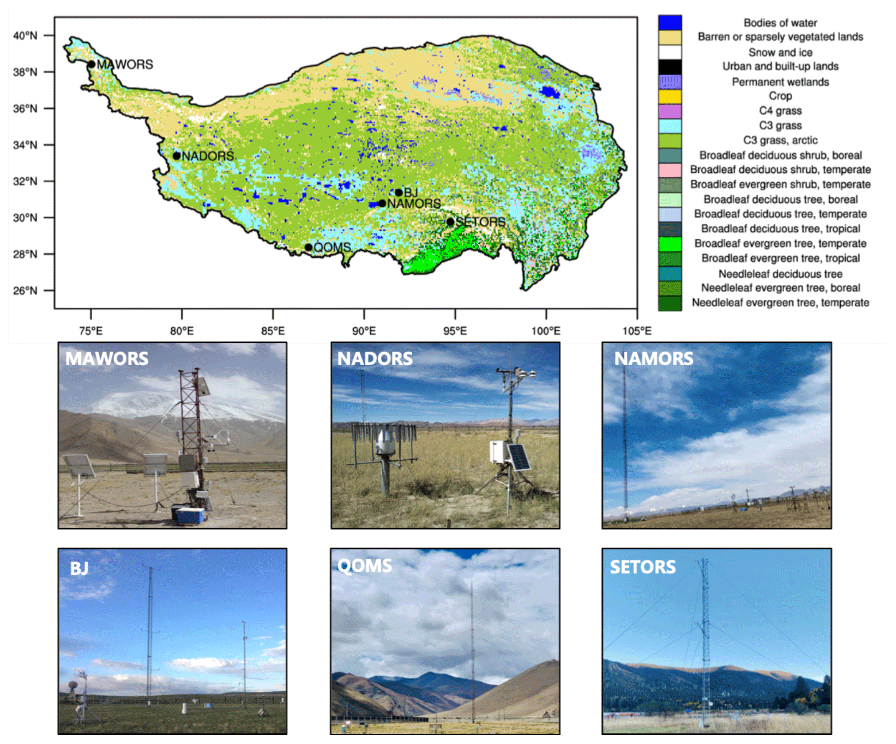
Figure 1 The integrated land–atmosphere observation network on the TP. At each site, the near surface atmospheric conditions are sampled with multilayer wind speed and direction, air temperature and humidity instruments. Surface pressure, precipitation and four-component surface radiation fluxes are also measured. Vertical profiles of soil temperature and soil moisture content are monitored by multilayer temperature probes and water content reflectometers. An open path eddy covariance turbulent measurement system is installed at each site to provide continuous monitoring of the vertical turbulent fluxes within the atmospheric boundary layers (the data source of the land cover map in the top of this figure is Ran and Li, 2019).

The MAWORS station is located in the region where the atmospheric circulation was influenced by the westerly wind all year round. Soil at this station was predominately sandy soil and gravel with sparse and short grass. Large-scale modern glaciers are distributed around the station (the standard deviation of elevation within a kilometer around the station is 152.92 m, which is the highest among the six stations as shown in Table 1) and exert great influence on the local weather and climate. The observations from this station are of great significance for the study of interactions between westerly winds and monsoons and their effects on land–glacier–atmosphere changes, as well as changes in snow and ice resources.

Table 1 List of the geographic characteristics of the six sites.

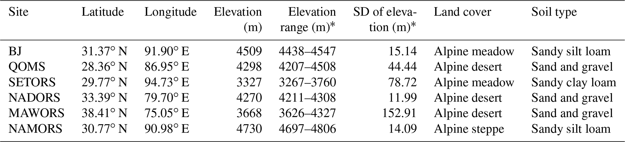
Note: * elevation range and standard deviation of elevation are calculated within a kilometer around the station based on the 30 m resolution ASTER DEM data (source: https://asterweb.jpl.nasa.gov/gdem.asp, last access: 20 August 2020)

The NADORS station was built in a flat and open mountain valley in the northwestern TP (with the lowest standard deviation of elevation). The land type here is Gobi Desert with very short grasses (about 1–2 cm) on the sandy soil and gravel surface. It is located at the convergence zone of the Indian monsoon and westerly wind, where these two atmospheric circulations interact intensively, making the NADORS as an excellent location for the study of westerly–monsoon interactions on the desert landscape.

The BJ site is located in a flat, open prairie except for the north, where there stand low hills (the standard deviation of elevation is 15.14 m). The site is well covered with vegetation, and the dense grasses are relatively high, with heights up to 5 cm. Soil at the site is predominantly sandy silt loam. The BJ site is an ideal place to observe the land–atmosphere interactions on the alpine meadow ecosystem.

The NAMORS station is located on the banks of Lake Nam Co, with the Nyainqentanglha Mountain behind. The land is covered by alpine meadows and the soil type is predominantly sandy silt loam, but the gravel content is high at 30–40 cm below the ground. As the lake has a significant influence on the atmospheric circulation in this region, it plays a certain role in regulating temperature variation and precipitation, etc. Thus, this station is an ideal place to measure the land–atmosphere interactions in the water–land–mountain mesoscale system.

The QOMS is situated at the bottom of the lower Rongbuk Valley, to the north of Mt. Everest. The surface is barren and the ground is relatively flat and open, with sparse and short vegetation. Sand and gravel are dominant here from the surface to deep soil. The Himalayas act as the channel for the exchange of energy and materials between surface and tropospheric atmosphere. Moreover, local circulation patterns, such as valley winds, link the near-surface atmosphere on the north side of Mt. Everest with the upper free atmosphere, making this region the best location for monitoring atmospheric conditions in the Northern Hemisphere.

The SETORS station lies in a mountain valley close to the forested southeastern TP (the terrain is highly heterogeneous but is not as complex as the MAWORS). It is covered by dense vegetation (mainly temperate needle-leaf trees and alpine meadows). The shallow soil here is well developed and the water-holding capacity of the soil is greatly enhanced due to the presence of organic matter, while the deep soil is predominantly gravel. The observations from the SETORS station are important for studying the water and heat transport along the alpine valleys by the South Asian monsoon, the alpine forest–glacier–atmosphere interactions, and the transport of hydrothermal components of the vertical belt in the mountainous regions.

This high and cold region observation network is an essential component of the meteorological observation platform over the TP, carrying out land surface process observations in areas that are typical in geography while currently lacking in situ observations. This network serves as key locations for field observations and experiments: in particular, for monitoring the interactions between geological processes and climate; for collecting first-hand, high-resolution records of modern environmental variations; and for monitoring land surface processes and atmospheric processes. The observation system at each station primarily includes the following four categories of measurements: meteorological variables either from the PBL tower or the AWS, solar radiation components, eddy covariance fluxes, and soil hydrothermal conditions. The meteorological instruments consist of up to five levels of wind speed and direction, air temperature, relative humidity instruments, surface air pressure and precipitation. The surface radiation components include the incoming and outgoing shortwave and longwave radiations. The open-path EC turbulent flux measurement system is used to sample the high-frequency vertical turbulent fluxes of the sensible heat flux, latent heat flux and carbon dioxide flux. Vertical profiles of soil temperature and soil moisture content are measured by multilayer temperature probes and water content reflectometers (five or six layers). A detailed list of the observation items and instruments can be found in Table 2. To ensure the accuracy and reliability of the observations, periodic inspection, maintenance and calibration are carried out by professional engineers. Meanwhile, all stations are manned except for in the cold winter season, and the instruments are checked and data are collected and processed regularly.

Table 2 Overview of the sensors used at each station.

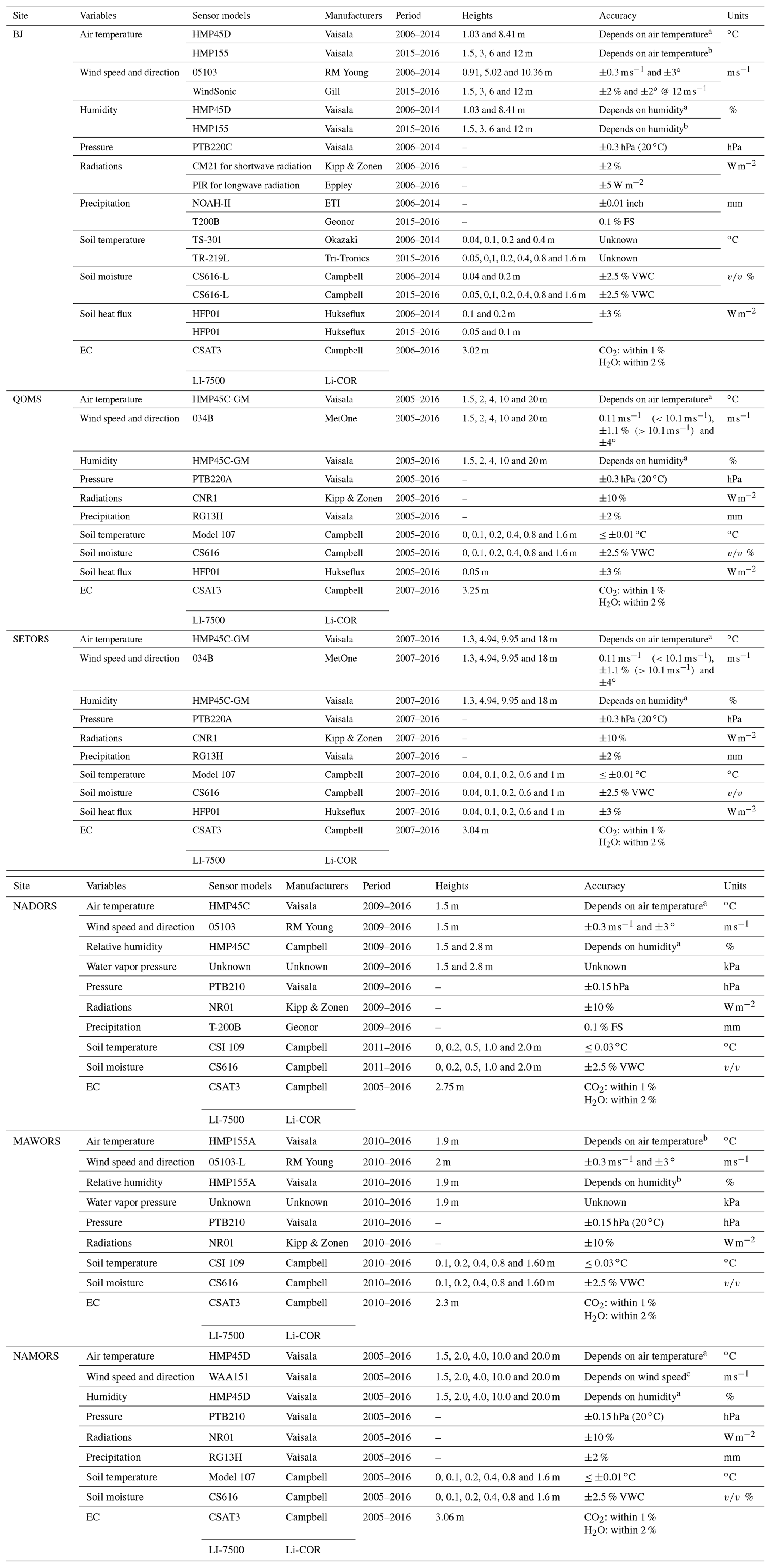
^a https://www.vaisala.com/sites/default/files/documents/HMP45AD-User-Guide-U274EN.pdf, (last access: 8 October 2020).
^b https://www.vaisala.com/sites/default/files/documents/HMP155-User-Guide-in-English-M210912EN.pdf, (last access: 8 October 2020).
^c https://www.techrentals.com.au/uploads/vai_waa151.pdf, (last access: 8 October 2020).

3 Integrated land–atmosphere interaction observations

3.1 Meteorological observations

To fully characterize the meteorological conditions and their vertical distributions in the surface layer, instruments were installed at several heights on a multi-layer PBL tower (QOMS, NAMORS, SETORS and BJ). For stations without the PBL tower, meteorological variables are recorded by a one-layer AWS at MAWORS and two-layer AWS at NADORS. The layer arrangements of sensors are not the same at these six stations. For example, five layers of wind speed and wind direction anemometers, air temperature and humidity probes were installed at QOMS and NAMORS; four layers of sensors were installed at SETORS; for BJ, three layers of wind and two layers of air temperature and relative humidity probes were available during 2006–2014, while four levels of these measurements were provided during 2015–2016 (see Table 2 for details). As well as this, a surface pressure barometer and precipitation gauge are available at all the stations except MAWORS, where precipitation is not measured. The meteorological elements of each station are detailed in the following sections, starting with the observation infrastructure, and followed by variations of the climatological average meteorological variables (except for wind direction and precipitation) at the lowest level of each station. We should note that the term “climatological” here does not strictly follow the definition recommended by the World Meteorological Organization (WMO), for which averages are based on 30 years of data. Here, “climatological” refers to the period for which variables are available at each station. At BJ, the climatological averages of wind speed, air temperature, relative humidity and pressure were calculated from 2006 to 2014.

3.1.1 Wind speed and wind direction

Wind speed and wind direction were monitored using non-heated anemometers at NADORS, MAWORS, NAMORS, QOMS and SETORS, while using heated ultrasonic anemometers at BJ. At NADORS and MAWORS, the horizontal wind variations were monitored at heights of 1.5 and 2 m above the ground, respectively. At the NAMORS and QOMS, wind speed was measured at heights of 1.5, 2, 4, 10 and 20 m, while wind direction was only available at 1.5, 10 and 20 m. At SETORS, wind speed and wind direction were measured at four levels (1.3, 4.94, 9.95 and 18 m). At BJ, three layers of wind speed (at heights of 0.91, 5.02 and 10.36 m) and one-layer wind direction (at a height of 10.36 m) were available from 2006 to 2014 while the wind speed and wind direction were available at four levels (1.5, 3, 6 and 12 m) during 2015–2016.

The climatological averaged wind speeds at diurnal, daily and monthly scales are shown in Fig. 2a–c. Clear inner diurnal variations were observed, characterized by a maximum in the afternoon and a constant wind speed in the early morning and throughout the night. At the diurnal scale, wind speed at SETORS showed the lowest diurnal variation throughout the year, while that at BJ showed the largest variations (the multi-year average here reached 8.13 m s⁻¹ in the afternoon in January). At BJ, MAWORS, NADORS and NAMORS, the variations in wind speed in winter (December, January and February) were larger than those in the other seasons, while the greatest variability was observed in spring and early summer at QOMS. Significant differences exist in the climatological averaged monthly wind speeds at all stations, except at SETORS, where the wind speed ranged only from 0.79 to 1.26 m s⁻¹. Generally, the wind speed was relatively lower during the monsoon season than the non-monsoon periods, particularly at QOMS, BJ, NAMORS and MAWORS, where wind speeds in winter were the highest throughout the year, while the largest values of wind speed were observed in spring at NADORS.

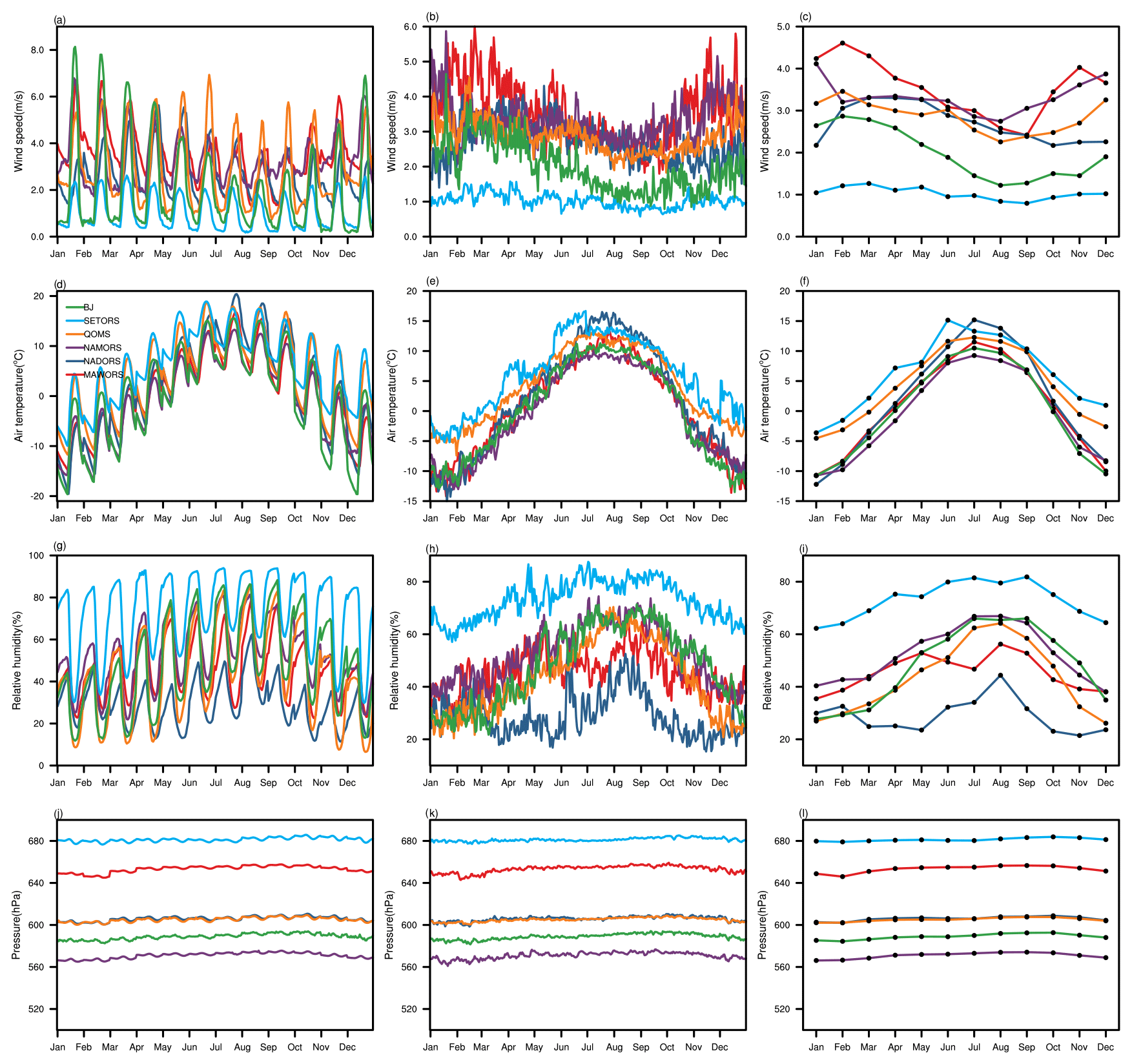
Figure 2 The climatological averages of the lowest level of wind speed, air temperature, relative humidity and surface pressure at diurnal (left), daily (middle) and monthly (right) scales. For sites except BJ, the climatological mean of each variable was calculated based on all the available observations; for BJ, only the observations during the period of 2006–2014 were used.

3.1.2 Air temperature

Air temperature is available at different heights at NAMORS (1.5, 2.0, 4.0, 10 and 20 m), QOMS (1.5, 2.0, 4.0, 10 and 20 m), SETORS (1.3, 4.94, 9.95 and 18 m) and MAWORS (1.9 m). Air temperatures were recorded at a single height of 1.5 m at NDORS and two heights of 1.03 and 8.41 m at BJ during 2006 to 2014. Identical to the wind sensors configuration, an air temperature gradient observation system with temperature probes at four heights (1.5, 3.0, 6.0 and 12 m) was used at BJ since 2015.

The multi-year monthly averaged diurnal variations of air temperature (Fig. 2d) show that the values at NAMORS, QOMS and MAWORS were below 0 ^∘C in November, December, January and February. At BJ, the air temperature in January were below 0 ^∘C and the maximum values in December and February were also around freezing temperature (1.17 and 0.72 ^∘C, respectively). As shown in Fig. 2e, the minimum daily air temperatures at BJ, MAWORS, NAMORS and NADORS dropped below 0 ^∘C from mid-October until the end of March or early April of the following year, but they were approximately 5 ^∘C higher at QOMS and SETORS. These differences in the variations in daily mean air temperature among stations are clearly shown in Fig. 2f. In summer (June, July and August), the average daily and monthly air temperature at the lowest level at NADORS was the highest among the six stations. Moreover, a wide variability was detected in the multi-year daily mean air temperatures at SETORS, especially in late March to early April, late May and early December (Fig. 2e). This abnormal variation indicates an instrument failure in the air temperature observations at 1.3 m at SETORS. Although this issue has been detected, the air temperature data provided at present are in raw format without any post-processing applied. Consequently, careful inspection is crucial when air temperature observations are required. In subsequent work, stricter data quality controls will be applied to detect problematic data and quality flags will be provided for each observational element.

3.1.3 Humidity

The heights of the humidity sensors are the same as those of the air temperature probes. Besides the relative humidity, up to four layers of water vapor pressure observations are also available at MAWORS (1.9 m), NADORS (1.5 and 2.8 m) and BJ (only available for the period 2015–2016, at 1.5, 3, 6 and 12 m); the heights of the water vapor pressure sensors at BJ are consistent with the heights of air temperature during the period from 2015 to 2016. Note that the unit of water vapor pressure is kilopascals (kPa) at MAWORS and NADORS, while it is 0.1 hPa at BJ.

The relative humidity showed obvious diurnal variations, peaking in the afternoon (Fig. 2g). Compared with the magnitude of diurnal variations in summer, the diurnal range of relative humidity at SETORS in winter and spring was much greater, reaching 50 %, and the maximum value of the average diurnal cycle of relative humidity was about 80 %, which was also significantly higher than those at other stations. In contrast, the diurnal variability during the monsoon season was much smaller than those at BJ, QOMS, NAMORS and MAWORS. The monthly relative humidity was lowest at NADORS; however, there was a marked increase in summer due to the transition of midlatitude westerlies to the Asian summer monsoon. Differences in humidity among the six stations presented in the diurnal and daily relative humidity records were clearly reflected in the seasonal variations at the monthly scale.

3.1.4 Air pressure

Barometers produced by Vaisala were installed at each station. Compared with variations in wind speed, air temperature and relative humidity, the diurnal and seasonal variations in air pressure were not obvious (Fig. 2j–l), and pressure remained at a relatively stable level throughout the year. Air pressure is elevation-dependent amongst the six stations, with the highest value at SETORS and the lowest value at NAMORS, while consistent diurnal and seasonal variations were found both at QOMS and NADORS, which are of similar altitude.

3.1.5 Precipitation

Precipitation is measured at all stations except for MAWORS, either with tipping buckets or weighting gauges. At BJ and NADORS, the cumulative precipitation is recorded, while the total half-hourly precipitation is recorded at NAMORS, QOMS and SETORS. For the cumulative precipitation, negative growth resulting from the evaporation from the rain gauge can seriously affect the measurement accuracy. Moreover, large errors can be introduced in the precipitation time series by wind-induced under-catch, wetting loss, evaporation loss and underestimation of trace precipitation amounts; it is difficult to apply bias correction to account for these losses (Goodison et al., 1998). While precipitation data are extremely valuable, accurate measurement is notoriously difficult due to the large errors mentioned above, particularly in cold regions such as the TP. Therefore, in the released datasets, the precipitation data are provided in raw format without any post-processing, which might potentially be underestimated; thus further bias correction or data selection is necessary before the precipitation observations are used.

3.2 Surface radiations

Surface radiations are an important component of surface meteorological observations and are released as a separate category. A four-component radiation flux observing system was installed at each station. The surface radiation flux monitoring system consists of upward and downward pyranometers for outgoing and incoming shortwave radiation flux, and upward and downward pyrgeometers for outgoing and incoming longwave radiation flux. A separate measurement system (CM21 and PIR) was used to measure the radiation fluxes at BJ station, while the K&Z CNR1, consisting of a pyranometer and pyrgeometer pair that can measure shortwave and longwave radiation, respectively, was used at other stations.

Figure 3a–c shows that the diurnal variations in downward shortwave radiation flux at QOMS were the highest among the six stations, and the largest amplitude occurred in April with a range of 0–1027 W m⁻². In winter, the MAWARS showed the smallest diurnal variation in downward shortwave radiation flux, while the variations at SETORS were the smallest in other seasons. When combined with the relatively higher solar radiation flux in this area, variations in upward shortwave radiation flux at QOMS were relatively high (Fig. 3d). The multi-year averaged daily series showed wide fluctuations in upward shortwave radiation at NAMORS in September and October, as well as at QOMS in the winter and spring (Fig. 3e), which may result from high fractional snow cover during these periods. In the early stage of the summer monsoon, the downward shortwave radiation decreased gradually with increasing cloud cover, as a result of the increase in moisture in the upper atmosphere. Both the incoming and outgoing longwave radiation flux at each station (Fig. 3g–i and j–l, respectively) showed significant seasonal variations, with high values in summer and low values in winter because of its dependence on air and ground temperatures. Upward longwave radiation flux at QOMS was higher than that at other stations (excluding SETORS) except in July and August when NADORS showed the largest values (Fig. 3k and l; note the time series of longwave radiation fluxes at SETORS are not plotted in Fig. 3 because of monitoring problems, but some of the remaining valid observations show that the longwave radiation fluxes at SETORS are the largest among all the stations). These differences showed high consistency with the differences in uppermost layer soil temperature as shown in Fig. 5d–f.

Figure 3 Same as Fig. 2, but for the climatological average of the downward and upward solar radiation (Rsd and Rsu), and incoming and outgoing longwave radiation (Rld and Rlu).

3.3 EC data

The EC technique was applied to provide high-quality and continuous surface turbulent flux data for momentum and sensible and latent heat. The EC system comprises a sonic anemometer (CSAT3, Campbell Scientific, Inc.) and a fast-response gas analyzer (LI-7500 open-path gas analyzer, Li-COR). All of the turbulence data were processed and quality-controlled using the TK3 software package (Mauder and Foken, 2011); the main processing procedures were as follows: excluding physically invalid values and spikes, revising the time delay of the high-frequency water vapor and carbon dioxide sampling, planar fit coordinate rotation, correction of the loss of frequency response, correction of the ultrasonic virtual temperature and density fluctuations. The quality of each turbulent flux data series was evaluated by using the stationarity test and integral turbulence characteristics test. By combining the quality flags for stationarity and the integral turbulence characteristics test, a final quality flag (1–9) was assigned to each specific turbulent flux value except those for BJ, where classes 0–2 were used. Classes 1–3 (or 0 at BJ) indicate good quality suitable for fundamental research purposes, and classes 4–6 (1 at BJ) indicate suitability for general use, such as long-term analysis. Classes 7–9 (2 at BJ) should be discarded. The multi-year diurnal variation and seasonal variation of sensible and latent heat flux were calculated based on the data with medium or higher quality.

3.3.1 Sensible heat flux

As can be seen from the diurnal variations of sensible heat flux in Fig. 4a, the sensible heat fluxes at all stations were negative at night. During the period from March to October, the atmospheric heating effect on the ground at NADORS was the strongest during the night, while the magnitude of diurnal variation in the sensible heat flux was the lowest here among the six stations from April to September. The variations in sensible heat flux (Fig. 4a–c) show that prior to the monsoon season, the sensible heat flux was the main consumer of surface available energy, and then the diurnal variation in sensible heat flux decreased significantly with the onset of summer monsoon and was comparable to the latent heat flux. In other words, sensible heat flux exchanges prevail during the pre-monsoon periods. The timing of the onset of decreasing sensible heat flux following the spring maximum varied, occurring earliest at SETORS and NAMORS, followed by BJ and NADORS. Influenced by the interactions between the midlatitude westerlies and the summer monsoon, the summer sensible heat fluxes were significantly lower than those in spring at all stations.

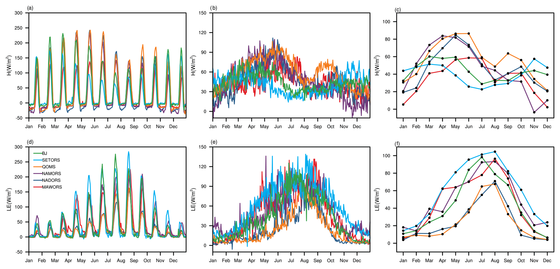
Figure 4 Same as Fig. 2, but for the climatological average of the sensible heat flux (H) and latent heat flux (LE) variation.

3.3.2 Latent heat flux

In contrast to the bimodal pattern of the seasonal variations in sensible heat flux, the seasonal variation in latent heat flux revealed a unimodal pattern; that is, the latent heat flux was small during the pre-monsoon period, and during monsoon outbreaks, it increased rapidly as precipitation became frequent and the surface soil turned wet. The latent heat flux then increased gradually, and it became comparable to the sensible heat flux during the summer monsoon period. A comparison of the seasonal variation of sensible heat flux (Fig. 4c) and latent heat flux (Fig. 4f) reveals that the latent heat flux was more significant to the sensible heat flux during the Asian summer monsoon season. During this period, the latent heat flux predominated in the surface energy budget (excluding the QOMS and NADORS), and the magnitudes of diurnal variations of latent heat flux were greatest at SETORS and BJ, and weakest in the desert landscapes of QOMS and NADORS (Fig. 4d).

3.3.3 Carbon dioxide flux

The carbon dioxide flux is an important component of the atmospheric carbon balance and is a very important variable in the study of global climate change. As one of the key components of the EC monitoring system, the observed carbon dioxide fluxes at each station are provided through the density correction and frequency response correction applied by the TK3 software package (Mauder and Foken, 2011). A previous study has reported that the self-heating of the infrared gas analyzer in the open-path EC system can cause notable differences in temperature between the observation path and the ambient air, which may result in signal distortion (Burba et al., 2008); therefore, it is necessary to apply a specific correction to the carbon dioxide flux data to eliminate the heating impact and to accurately reveal the intensity of carbon dioxide exchange in the TP ecosystem (Zhu et al., 2012). However, the heating effect of the instrument was not been considered in the carbon dioxide flux data provided in this paper; more detailed information can be found in the studies of Burba et al. (2008) and Zhu et al. (2012). When these data are used in studies of carbon dioxide exchange or related works (for example, estimating the net ecosystem production and its components), this specific correction of the data is needed to fully account for the impact of instrumental heating on observations.

3.4 Soil hydrothermal observations

3.4.1 Ground surface temperature

Ground temperatures at NADORS, SETORS and BJ are provided in this dataset. The variations in ground temperature show the weakest diurnal variations at BJ and the strongest at SETORS, where the ground temperature during the night was highest among the six stations. On the daily scale, the daily mean ground temperature at BJ was lower than that at SETORS and NADORS throughout the year, although its amplitude of the diurnal cycles was larger than that at the other two stations owing to the lower night-time temperatures (Fig. 5a). Daily mean and monthly ground temperatures at BJ dropped below 0 ^∘C during all months from October to April.

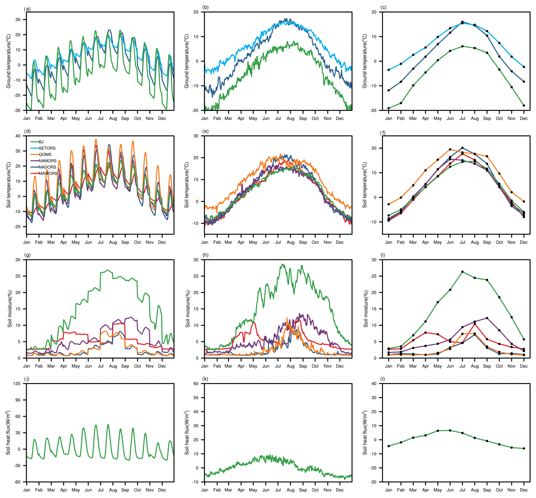
Figure 5 Same as Fig. 2, but for the climatological average of ground temperature and first-layer (except for the observations at depths of 0 cm) soil temperature, soil moisture and soil heat flux.

3.4.2 Soil temperature and soil moisture

Soil temperature and soil moisture are key physical quantities characterizing the land surface conditions and play important roles in controlling the energy and mass interactions between land and the overlying atmosphere. To capture the continuous, real-time soil thermal and soil moisture conditions on different ground surfaces of the TP, five layers of soil profile sensors (soil temperature probes and water content reflectometers) were installed at SETORS (4, 10, 20, 60 and 100 cm), MAWORS (10, 20, 40, 80 and 160 cm) and NADORS (0, 20, 50, 100 and 200 cm). At NAMORS and QOMS, soil temperature and soil moisture were observed at depths of 0, 10, 20, 40, 80 and 160 cm. At BJ, soil temperature and soil water content were measured at four depths (0, 4, 10, 20 and 40 cm) during 2006–2014, and then at six depths (5, 10, 20, 40, 80 and 160 cm) during 2015–2016.

Figure 5a–f and g–i demonstrates the variations of soil temperature and soil moisture, respectively, in the uppermost layer of each station (i.e., the top layer after excluding observations at a depth of 0 cm). Specifically, these were at depths of 4 cm at SETORS and BJ; 10 cm at MAWORS, NAMORS and QOMS; and 20 cm at NADORS. Soil temperatures in the shallow layers show obvious variation at the diurnal scale and are highly consistent with the variations in air temperature. The soil water content quickly responded to precipitation with an obvious increase with the onset of summer monsoon, particularly at BJ. Wiring problems at SETORS caused erroneous soil temperature and soil water content readings in all layers, which seriously affected the reliability of the respective observations. Although the two variables from SETORS are available in this dataset, data quality control and correction are needed.

3.4.3 Soil heat flux

Soil heat flux was measured by soil heat flux plates buried at BJ (10 and 20 cm for 2006–2014, 5 and 10 cm for 2015–2016), QOMS (10 cm) and SETORS (4, 10, 20, 60 and 100 cm). All the available soil heat flux data at each depth are released through this data descriptor. Due to abnormal fluctuations of the top-layer soil heat flux at QOMS and SETORS at both the diurnal and daily scale, only the variations in top-layer soil heat flux at the BJ site were presented in Fig. 5. The soil heat flux at BJ showed that it was usually relatively small and had evident diurnal and seasonal variations.

4 Data availability

Raw data were converted from binary mode to ASCII mode, and then key variables were extracted and saved as comma-separated values (.csv format). The CSV format was chosen as it is one of the most widely supported structured data formats in scientific applications. The plausible value check, time consistency check and internal consistency checks were applied to ensure the accuracy and reliability of the observations. However, to retain the observations in their original form as much as possible, there is no further process taken except for replacing outliers with missing value (NaN). Data consistency check procedures were applied to ensure the accuracy and reliability of the observations, but the data quality flag is not available for the moment. For turbulent flux data, classes 1–3 (0 for BJ station) were recommended for fundamental research, such as surface energy balance analysis. Classes 4–6 (1 for BJ station) can be used in continuously running systems or for long-term analysis. Some time series of observations should be used with caution (for example, the soil hydrothermal data in SETORS), as anomalous changes or values were detected. In this case, further procedures such as bias correction or data selection are required. The local time was used in all the data files (UTC+8). All datasets presented and described in this article have been released and are available for free download from the Science Data Bank (https://doi.org/10.11922/sciencedb.00103, Ma et al., 2020) and the TPDC (https://doi.org/10.11888/Meteoro.tpdc.270910, Ma, 2020). Special compressed files were designated for each station with four categories: turbulent flux data (FLUX), gradient meteorological data (GRAD), soil hydrothermal data (SOIL) and radiation data (RADM). Meanwhile, the data integrity of each variable was also provided every year, with the value of 100 indicating complete continuous data, with no missing data. The heat maps shown in the Appendix are used to provide the data integrity information. These figures are very useful as they provide an intuitive depiction of the availability of each variable, facilitating data selection when analyzing land–atmosphere interactions and the structure of PBL, driving land surface models, or evaluating model results.

5 Summary

As in situ observations are scarce yet invaluable in cold regions, the model parameterization schemes are generally developed and evaluated based on a small number of sites, of which very few are located in high mountainous regions. Current numerical models suffer from a poor representation of the cold-region processes, particularly on the TP (Xia et al., 2014; Toure et al., 2016; Orsolini et al., 2019; Xie et al., 2019). Long-term, high-quality and high-temporal-resolution observational data in the Third Pole region are not only extremely scarce, but are also very important for a deeper understanding of the key land surface processes. In this paper, a suite of land–atmosphere interaction observations from the integrated observation network over the TP is presented. Compared with previously open-access daily meteorological observations over the TP, this dataset provides the most comprehensive and high-quality continuous in situ observations, with the highest temporal resolution (hourly) to date. Therefore, this fine-resolution data product can help to promote comprehensive scientific understanding of the interactions among the multi-sphere coupled systems over the TP and even the globe, to quantify uncertainties in satellite and model products, to assess the biases and gaps existing between the model simulations and reality, and to facilitate the development and improvement of land surface process models in cold regions. We believe that the datasets presented in this paper will contribute to these research areas and that they will be widely used in model development and evaluation.

Appendix A: Annual data integrity

Figures A1–A4 illustrate the annual data integrity of the gradient meteorological observing elements at different level, surface radiation fluxes, soil hydrothermal observations and turbulent flux observations, respectively. The value of 100 indicates complete continuous data, with no missing data.

Figure A1 The annual data integrity of the gradient meteorological observing elements at different levels, with a value of 100 indicating complete continuous data, with no missing data. WS and WD represent wind speed and direction, respectively, followed by heights of each level with the underline symbol as connection. Ta refers to the air temperature. Relative humidity and water vapor pressure are expressed using RH and Vapor, respectively.

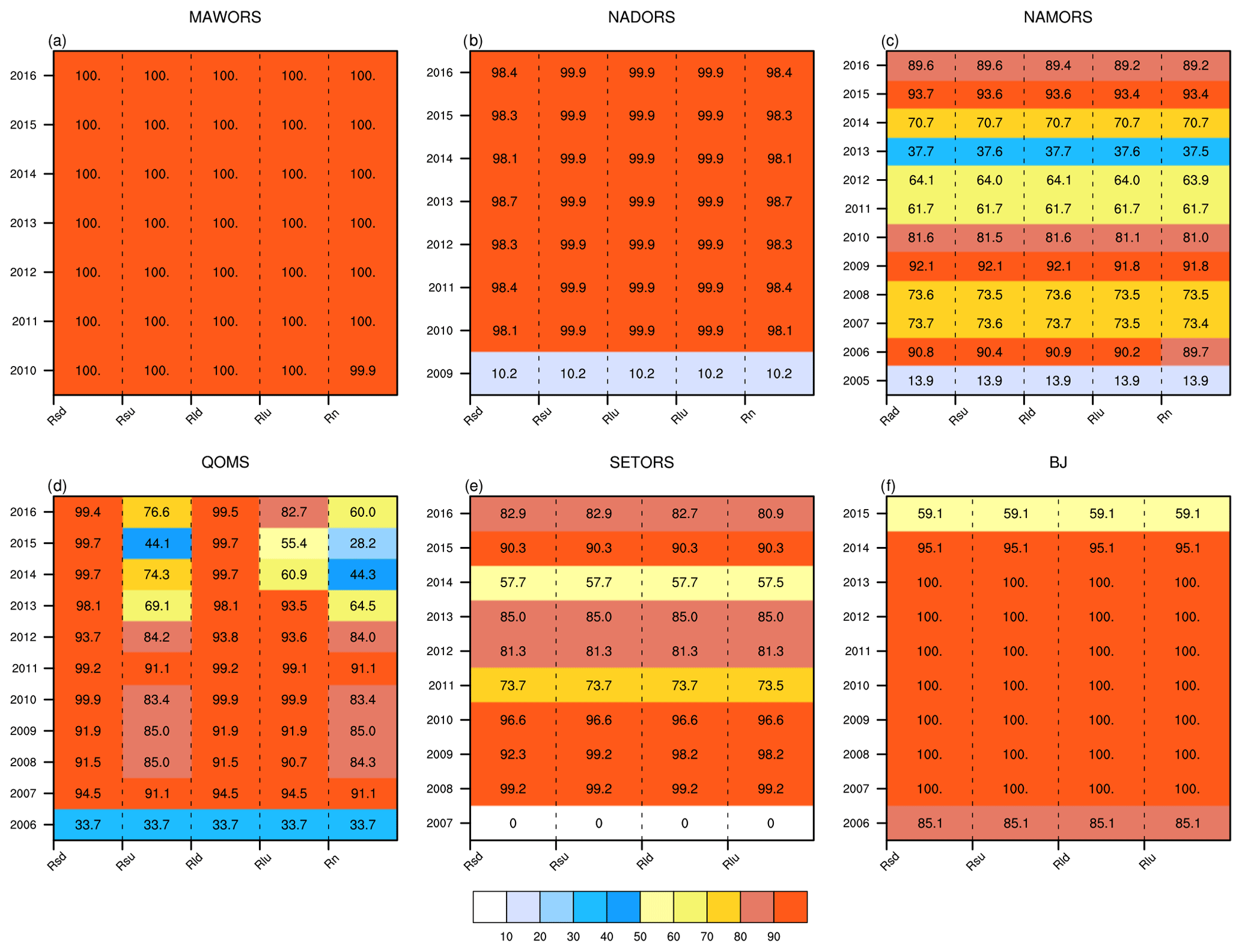
Figure A2 Same as Fig. A1, but for the surface radiations. Rsd and Rsu represent the incoming and outcoming solar radiation, respectively; Rld and Rlu refer to the downward and upward longwave radiation. The net radiation is expressed using Rn.

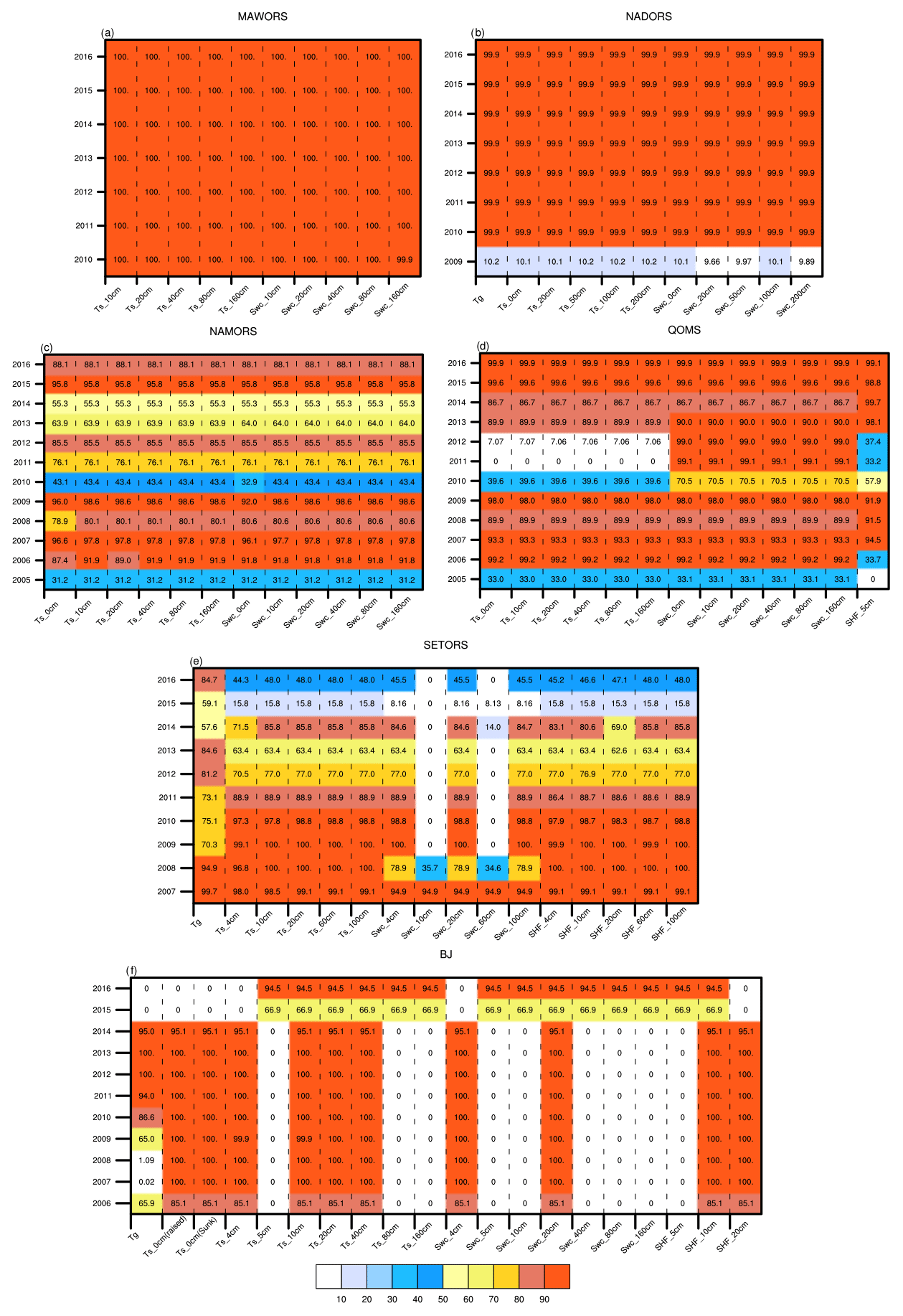
Figure A3 Same as Fig. A1, but for the soil hydrothermal observations. Ground temperature is represented by Tg, and the soil temperature and soil water content are expressed with Ts and SWC, respectively; SHF refers to the soil heat flux.

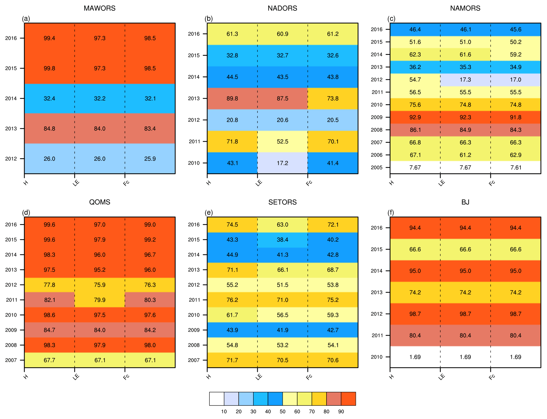
Figure A4 Same as Fig. A1, but for the turbulent flux observations. H represents sensible heat flux, LE represents latent heat flux, and the CO₂ flux is expressed with Fc.