the Creative Commons Attribution 4.0 License.
the Creative Commons Attribution 4.0 License.
 | 18 Nov 2020
Trade-wind clouds and aerosols characterized by airborne horizontal lidar measurements during the EUREC4A field campaign
Patrick Chazette
Julien Totems
Alexandre Baron
Cyrille Flamant
Sandrine Bony
From 23 January to 13 February 2020, 20 manned research flights were conducted over the tropical Atlantic, off the coast of Barbados ( N, W), to characterize the trade-wind clouds generated by shallow convection. These flights were conducted as part of the international EUREC4A (Elucidating the role of cloud–circulation coupling in climate) field campaign. One of the objectives of these flights was to characterize the trade-wind cumuli at their base for a range of meteorological conditions, convective mesoscale organizations and times of the day, with the help of sidewards-staring remote sensing instruments (lidar and radar). This paper presents the datasets associated with horizontal lidar measurements. The lidar sampled clouds from a lateral window of the aircraft over a range of about 8 km, with a horizontal resolution of 15 m, over a rectangle pattern of 20 km by 130 km. The measurements made possible the characterization of the size distribution of clouds near their base and the presence of dust-like aerosols within and above the marine boundary layer. This paper presents the measurements and the different levels of data processing, ranging from the raw Level 1 data (https://doi.org/10.25326/57; Chazette et al., 2020c) to the Level 2 and Level 3 processed data that include a horizontal cloud mask (https://doi.org/10.25326/58; Chazette et al., 2020b) and aerosol extinction coefficients (https://doi.org/10.25326/59; Chazette et al., 2020a). An intermediate level, companion to Level 1 data (Level 1.5), is also available for calibrated and geolocalized data (https://doi.org/10.25326/57; Chazette et al., 2020c).
- Article
(13511 KB) - Full-text XML
- BibTeX
- EndNote


Subtropical regions play a major role in the radiation balance of the Earth due to their dry free troposphere and their ability to emit a large amount of heat to space (Pierrehumbert, 1995). Within the marine boundary layer, these regions are associated with low-level clouds that also contribute to cool the Earth through the reflection of sunlight. In the trade-wind regimes, the prevailing clouds are shallow cumuli (Norris, 1998). They are so ubiquitous that their response to changes in the environment has the potential to greatly influence the global radiation budget. In climate models, the differing responses of these clouds to global warming has been identified as one of the leading causes of uncertainty in climate sensitivity (Bony and Dufresne, 2005; Brient et al., 2016; Medeiros et al., 2015; Vial et al., 2017). The models that predict a significant decrease in shallow cumuli with warming predict a higher climate sensitivity than the models that predict weak or no change. To assess the credibility of climate projections, it is thus necessary to understand how these clouds interact with their environment.
This was one of the main motivations of the EUREC4A (Elucidating the role of clouds-circulation coupling in climate) field campaign which took place in January–February 2020 over the western tropical Atlantic, west of Barbados (Stevens et al., 2020). This experiment was originally designed to test our understanding of low-cloud feedbacks (Bony et al., 2017), especially the physical processes that control the cloud fraction around cloud base, where climate models predict the largest changes in cloudiness with warming. In addition, clouds in the trade-wind regimes exhibit prominent forms of convective organization (Stevens et al. 2020), and the mesoscale cloud patterns depend on environmental conditions and influence the reflection of sunlight (Bony et al., 2020). The question thus arises as to whether changes in the mesoscale organization of clouds might play a role in low-cloud feedbacks (Nuijens and Siebesma, 2019). Answering this question constitutes another key objective of the EUREC4A campaign. To address these issues, EUREC4A aimed at characterizing the field of trade cumuli, in particular the horizontal cloud coverage around cloud base, the spatial arrangement and the size distribution of clouds, through complementary platforms and instruments, including airborne lidars.
Indeed, from a remote sensing point of view, shallow cumuli count among the most challenging clouds. They are small, broken and sometimes very optically thin, so their detection by radiometry can be difficult. In contrast, lidars have the potential to detect them much better (Liou and Schotland, 1971; Spinhirne et al., 1982). Space-borne lidars associated with missions such as LITE (Lidar In-space Technology Experiment, Winker et al., 1996), GLASS (Geoscience Laser Altimeter System; Palm et al., 2005; Spinhirne et al., 2005), CALIPSO (Cloud-Aerosol LIdar with Orthogonal Polarization; Winker et al., 2003) or more recently CATS (Cloud-Aerosol Transport System, Yorks et al., 2016) have even revolutionized our knowledge of the global distribution of clouds (Berthier et al., 2008). However, cloud observations from ground-based, airborne or satellite lidar technology were made at the nadir or zenith. Due to the overlap of cloud layers, this can make the observation of the cloud fraction around cloud base difficult. Moreover, the laser beam is so thin that it can only sample a tiny fractional area of the cloud field, especially in regions where the cloud fraction rarely exceeds 10 %. To increase the areal sampling of the cloud field and observe the cloud distribution at cloud base, EUREC4A introduced a new sampling approach, consisting in using an aircraft carrying a sidewards-staring lidar. This strategy was realized by implementing the Airborne Lidar for Atmospheric Studies (ALiAS) (Chazette et al., 2012b) with a horizontal line of sight in the ATR-42 of SAFIRE (the Service des Avions Français Instrumentés pour la Recherche en Environnment), using a modified lateral window on the aircraft. A horizontally looking cloud radar was also implemented on the same aircraft to complement the lidar observations and benefit from the lidar–radar synergy for the detection of clouds.
Horizontal lidar measurements have a great potential not only for the observation of clouds, but also for the characterization of aerosols. During the AMMA (African Monsoon Multidisciplinary Analysis; Redelsperger et al., 2006) campaign, Chazette et al. (2007) mounted a lidar on an ultralight aircraft and showed that if the atmosphere is horizontally homogeneous along the line of sight, horizontal shooting directly gives access to the extinction coefficient of aerosols without any hypothesis on their nature (Chazette et al., 2007). The same approach was used during the Dust and Biomass EXperiment (DABEX) with a combination between lidar measurements from an ultralight aircraft and in situ measurements from the UK FAAM aircraft (Johnson et al., 2008). Therefore, during EUREC4A the horizontal lidar measurements made from the ATR-42 were also used to characterize the marine boundary layer and long-range transport of aerosols within the free troposphere.
The goal of this paper is to present the flight strategy, measurements, data processing, and cloud and aerosol products derived from the horizontal lidar measurements made during the EUREC4A campaign. Section 2 presents the ALiAS lidar characteristics and Sect. 3 the implementation of the lidar in the ATR-42 aircraft. The flight plan and its decomposition into different phases are presented in Sect. 4. Section 5 describes the different levels of data processing and the cloud and aerosol products that constitute the final dataset. The conclusion is presented in Sect. 6 as well as how to access the data.
The ALiAS lidar was flown on board the ATR-42 (Fig. 1) of SAFIRE off the east coast of Barbados. Developed at LSCE (Laboratoire des Sciences du Climat et de l'Environnement) following a precursor instrument (Chazette et al., 2007), ALiAS is based on a frequency-tripled Nd:YAG laser (ULTRA-100) manufactured by Lumibird Quantel emitting at the wavelength of 355 nm. It satisfies eye safety requirements (EN60825-1) at the output window considering the characteristics given in Table 1 (emitted wavelength, pulse energy, repetition rate, beam diameter and pulse duration). The UV pulse energy is 30 mJ and the pulse repetition rate is 20 Hz. The acquisition system is based on a PXI-5124 (PCI eXtensions for Instrumentation) fast digitizer working at 200 MHz and 12 bits, without going through a pulse (photon) counter, leading to an initial resolution along the line of sight equal to 0.75 m. Using co- and cross-polarized channels relative to the linear polarization of the emitted radiation, ALiAS was designed to monitor the cloud, aerosol and hydrometeor distributions and dispersions in the low and middle troposphere from aircrafts. It was successfully used on board the Falcon 20 of SAFIRE to monitor and study the ash plume following the eruption of the Eyjafjallajökull volcano (Chazette et al., 2012b). The main characteristics of ALiAS are given in Table 1.
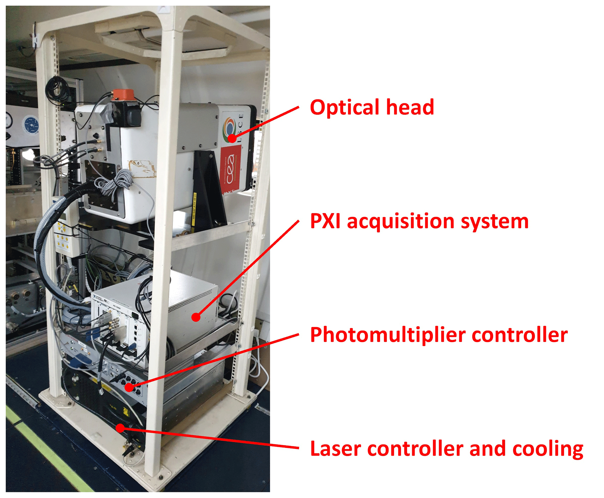
Table 1Characteristics of ALiAS on board the ATR-42 during the EUREC4A airborne campaign.

ALiAS was installed in the aft of the ATR-42 aircraft in an orientation that enabled a direct near-horizontal line of sight. Its orientation was measured the entire time by an inclinometer. The only possible solution for such an implementation, in compliance with aviation regulation, i.e. without complex modifications to the structure or aerodynamics of the aircraft, was to adapt an optical window with a custom frame inside an existing passenger window (Fig. 2). UV fused silica was chosen to ensure correct transmission of several useful lidar wavelengths (355, 532, 830, 1550, 2000 nm) at affordable cost. The frame being 244 mm × 164 mm, a 20 mm thickness was sufficient to ensure both a safety factor of ∼ 6 for mechanical resistance to air pressure difference and a wave front error below λ∕20 at 355 nm (Spark and Cottis, 1973). The window flatness was specified to λ∕4 at 633 nm, with an optical coating of 315 nm of MgF2 to reduce theoretical reflection losses to around 4 %. The ∼ 15∘ inclination of the window due to the curvature of the plane fuselage avoids harmful effects of the reflected beam inside the lidar, as long as the receiving aperture is above the emitting aperture, but extra beam tubing was found to be necessary to limit the impact of diffuse echoes on the sensitive lidar detectors.
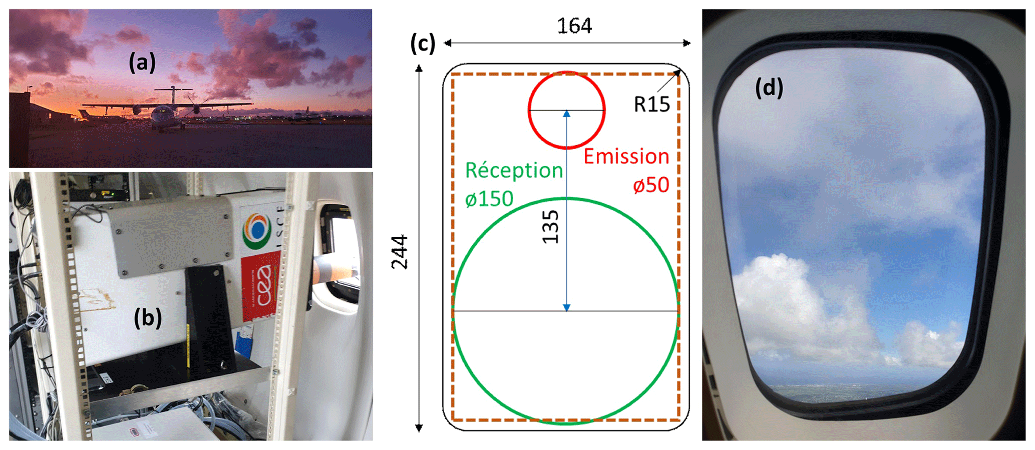
Figure 2Location of the ALiAS lidar in the ATR-42 (a). The lidar is placed horizontally (b) and the laser beam is guided to the MgF2 window (c) to avoid laser reflections. Window (c) has replaced a passenger window (d) in the back of the aircraft.
A specific study and certification were performed by SAFIRE itself to install the window at the back of the ATR-42 aircraft, on the starboard side. The optical head of ALiAS was already in a fibreglass container adapted to aircraft operation. As shown in Fig. 1, a standard aircraft-certified rack structure was fitted with a carrying structure for this container, and the elements of the lidar electronics were installed below, making the lidar system an easily mounted and self-contained unit. It was operated in flight from a passenger sitting in front of an in-flight checkpoint, allowing real-time validation of the cloud base altitude sampling.
The flight strategy was defined well before the intensive campaign and presented in Bony et al. (2017). It has been adapted to take into account the ATR-42 autonomy and the coordination with the other platforms involved in EUREC4A. The goal being to achieve a statistical sampling of the cloud fields, each flight repeated more or less the same flight plan, twice a day, independent of weather conditions.
On a given day of operation, the ATR-42 generally performed two flights, with each flight having a duration of ∼ 4 h. The take-off time of the ATR-42 was tightly coordinated with that of the High Altitude and Long-Range Research Aircraft (HALO) operated by DLR (Deutsches Zentrum für Luft- und Raumfahrt). The endurance of HALO (∼ 9 h) allowed the two ATR-42 flights to be conducted within the timeframe of a single HALO flight, taking into account the time for refuelling at Grantley Adams International Airport (GAIA) in between ATR-42 flights. Most of the ATR-42 flying time was spent off the east coast of Barbados within the so-called HALO circle, along which HALO released dropsondes and observed the atmosphere at nadir with a radar, a lidar and multiple radiometers (Stevens et al., 2019).
The flight strategy is illustrated in Fig. 3 for the flight on 26 January 2020. It was built along five major phases (see Table 2), which contributed to the multi-aircraft and statistical sampling strategy implemented during the field campaign. Note that during straight-line flights, the typical speed of the aircraft was ∼ 100 ms−1. Each phase was designed to address particular scientific requirements of the lidar and other remote sensing and in situ instruments composing the ATR-42 payload (radar, aerosol and cloud microphysics, water vapour stable isotopes using cavity ring-down spectrometry, turbulence).
-
On the way to the HALO circle, the ferry time was dedicated to perform an aircraft sounding up to 2.5–4.5 km above mean sea level (a.m.s.l.) to describe the vertical thermodynamical and dynamical structure of the lower atmosphere and obtain a first guess of the location of cloud and aerosol layers. Such an aircraft sounding was aimed at retrieving aerosol extinction coefficient and volume depolarization ratio profiles from the lidar measurements (see Sect. 5.3.2) and assess whether the upper part of the sounding was conducted in aerosol-free and/or cloud-free conditions. It is worth noting that several episodes of dust transport from West Africa were evident from the lidar data during the campaign.
-
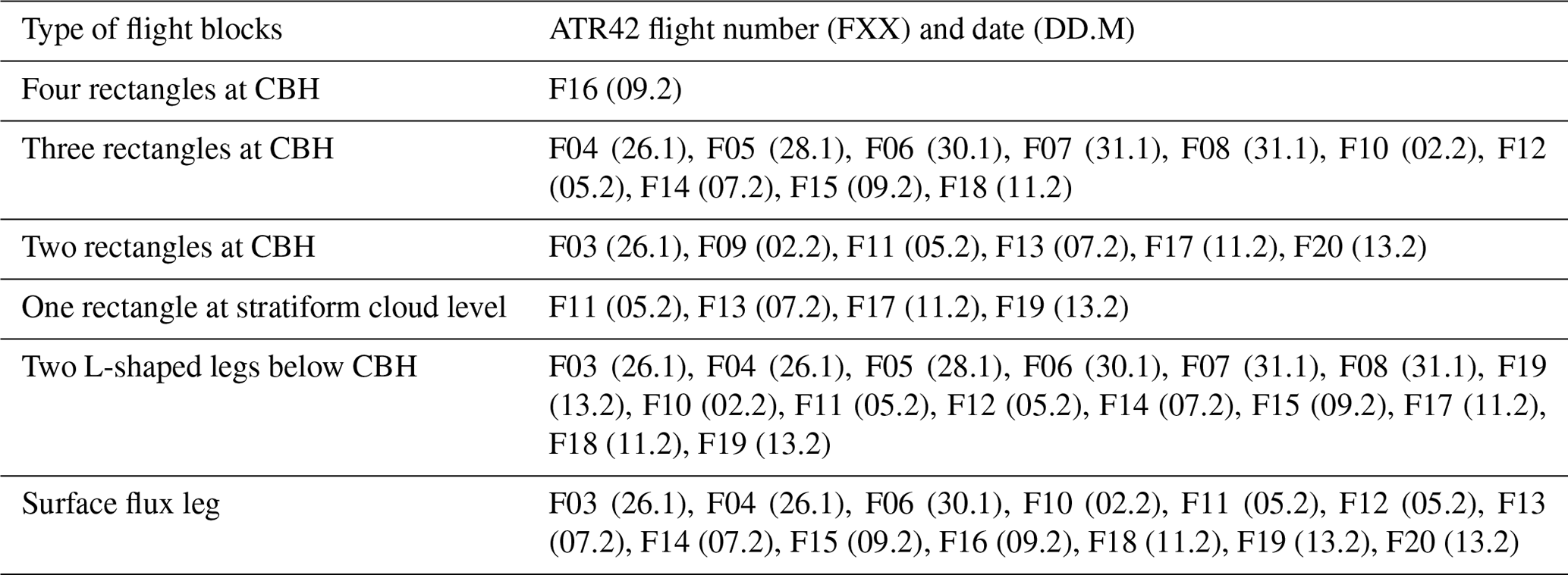
Upon arriving in the HALO circle, the ATR-42 started performing two or three north–south-oriented rectangles (roughly orthogonal to the trade winds), approximately 130 km long and 20 km wide. Each rectangle was flown in 45–50 min. The northwestern and southwesternmost corners of the rectangle were positioned 10 Nm (1 Nm = 1.852 km) to the west of the HALO circle. In the event that the ATR-42 circuit only included two rectangles, they were always performed around the cloud base height (CBH). When the circuit included three rectangles, on some occasions, the ATR-42 performed the first rectangle near the altitude of the ferry, mainly to sample stratiform clouds near the inversion level or the air just above. In such cases, the sideways-pointing lidar ALIAS allowed the characterization of the variability of aerosol-related extinction within the HALO circle in cloud-free conditions, or was used to obtain a cloud mask and further statistics on the properties of stratiform clouds, whenever they were present at the altitude of the flight. The second and third rectangles were always performed at CBH, to collect statistics on the spatial distribution of marine boundary layer clouds, measure the cloud base cloud fraction and provide a cloud mask. Figure 3 shows an example of a flight plan during which the three rectangles were performed at CBH on 26 January. On one occasion (on 9 February) the ATR-42 circuit comprised four rectangles performed at CBH (see Table 2),
-
After the rectangles, the ATR-42 performed two long L-shaped legs (of 20–25 min each) below CBH, one near the top and one near the middle of the subcloud layer. The first part of the L-shaped leg consisted of a ∼ 70 km long east–west-oriented run (approximately parallel to the mean trade winds), and the second part of the L, also ∼ 70 km long, was oriented perpendicularly to the first part. The return trip along the L-shaped legs was generally performed at the same altitude (see Fig. 3). These legs were essentially designed to characterize the turbulent structure of the marine boundary layer. In our case, they also allowed the characterization of the extinction and polarizing capability of aerosols present in the marine boundary layer,
-
At the end of the return trip along the second L-shaped run, the ATR-42 generally performed an ultra-low pass at 60 m above sea level for ∼ 10 min in order to measure turbulent heat fluxes and marine aerosols within the lower part of the planetary boundary layer.
-
The ATR-42 cruised back towards Barbados around 3 km a.m.s.l. (see Fig. 3). Meanwhile, the aircraft soundings allowed a second retrieval of aerosol extinction coefficient and volume depolarization ratio profiles which were used to assess how the geometrical and optical properties of aerosol layers evolved in the course of the flight.
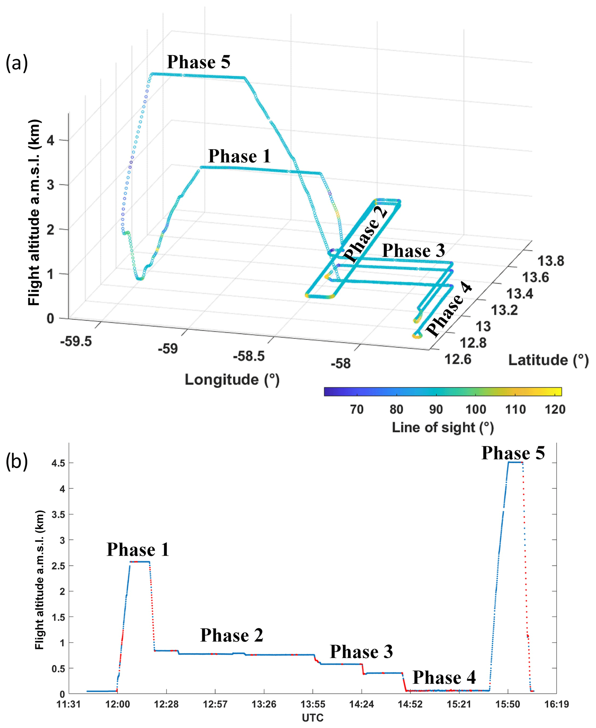
Figure 3Flight strategy of ATR-42 loading ALiAS for flight no. 04 on 26 January 2020. The five phases of the flight are highlighted.
The flight strategy was sometimes slightly adjusted based on the meteorological situation, e.g. depending on the presence of a stratiform cloud layer near the trade inversion level. The details on the ATR-42 flight blocks (rectangles, L-shaped legs, surface legs) are given in Table 2. It should be noted that prior to the beginning of Phase 2, a best-guess estimate of the CBH, assessed from multiple sources of information (radiosoundings launched from BCO (Barbados Cloud Observatory) and research vessels, dropsondes released from other aircraft), was provided to the ATR-42 scientists via the on-board chat capability. The flight altitude was then adjusted using real-time lidar echoes, cloud droplet counts from cloud microphysics probes, and visual observations by the pilots and the lidar operator through lateral windows.
Table 2Main flight blocks (rectangles, L-shaped legs, surface legs) for the ATR42 flights as well as flight dates.
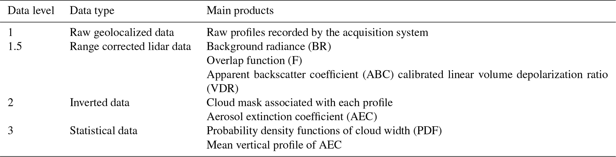
The data are presented from their raw form to the analytical products. They are classified into Level 1 to Level 3 as defined in Table 3. Up to Level 2 (included), lidar profiles are processed on an individual basis. The statistics performed on Level 2 data are gathered in the Level 3 data. Statistics are computed for all flights for the aerosol Level 3 products and for Phase 2 of the flights for the cloud products. The step from Level 1 data to the final products of Level 2 and Level 3 is schematized in Fig. 4. This section presents the steps taken to derive data products. The data recording format is detailed in Sect. 6. It should be noted that for Level 1 to Level 2, the location and attitude of the aircraft are also reported for each horizontal lidar profile.
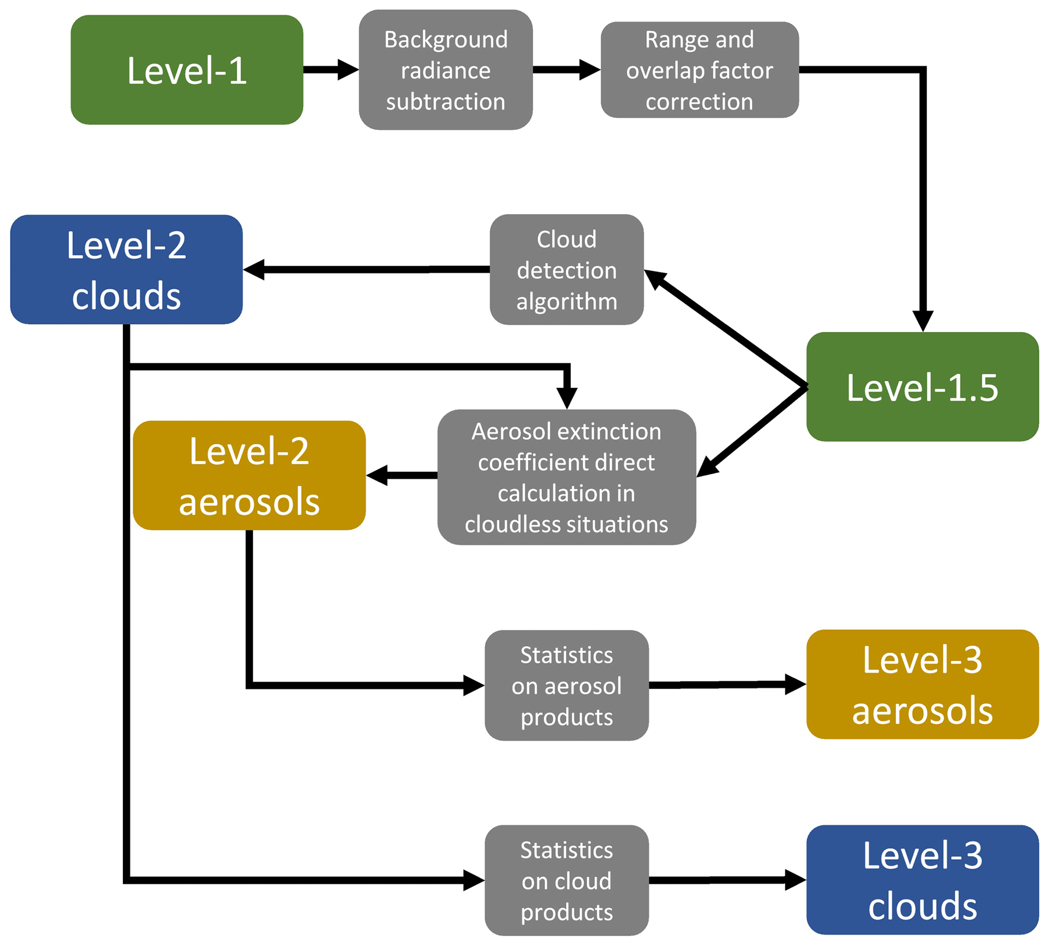
Figure 4Lidar data processing diagram starting from raw data (1) and calibrated data (Level 1.5) to products (Level 2 and Level 3). The grey cells summarize the actions to be implemented for the data processing. The green colour refers to data level in the pre-processing phase. Level 2 and Level 3 are subdivided into cloud (blue) or aerosol (orange) products.
5.1 Level 1
5.1.1 Description
Level 1 data are raw data expressed in volts. They are the result of time sampling at a frequency of 200 MHz. The raw sampling of the lidar profiles is 0.75 m along the line of sight, and an average over 50 shots is performed during the acquisition, corresponding to about one recording every 5 s (2.5 s averaging time and 2.5 s recording time). The first 2000 points are recorded before the laser emission is triggered. This offset makes it possible to record for each profile the contribution of the background sky radiance (BR) to the lidar signal (scattering of solar radiation in the atmosphere). This contribution must then be corrected during pre-processing.
The lidar signal S, for each polarization channel, of Level 1 data is expressed in the measurement configuration adopted for EUREC4A as
In this expression, the signal S depends on both the horizontal distance to the aircraft x and the flight altitude z. The system constant C is a function of various components of the lidar system such as the emitted energy and the quantum efficiency of the detectors (e.g. Shang and Chazette, 2015). The overlap factor F characterizes the overlap between the transmission and receiving fields of view and must be determined to exploit near-field data. As the laser beam propagates through the atmosphere, it is backscattered by air molecules (subscript m in the following), aerosols (subscript a) and/or clouds (subscript c) towards the receiving system. This interaction is characterized by the volume backscattering coefficient βk (k= m, a or c). The laser radiation is also attenuated by the atmospheric medium via the same actors, and this attenuation is quantified by the optical thickness τ, which is defined as a function of the extinction coefficient αk by the relation
Equation (1) assumes that the optical properties of molecules and aerosols remain constant along the line of sight. A deviation from this assumption can be easily verified on Level 1.5 data, as will be shown. In the presence of clouds, the heterogeneity is too strong for this hypothesis to be true.
As the laser beam emitted from the aircraft may not be completely horizontal, a viewing angle θ (with respect to the true horizon) must be taken into account. In addition to Level 1 data, the aircraft attitude parameters (pitch, roll, heading) that allow the assessment of θ are recorded, as well as the geo-positioning of the measurements (longitude, latitude and altitude).
5.1.2 Baseline check
Baseline distortion can significantly increase the rates of non-detection and/or false detection of cloud structures. Hence, in Level 1 data, potential drifts of the lidar signal baseline are checked for each flight, in order not to introduce any bias during data processing, mainly in the far field (i.e. beyond 4–5 km). This is done by comparing the BR from the pre-trigger with that computed in the far field, where the laser backscatter contribution becomes negligible, beyond 8 km in our case. As an example, Fig. 5 shows the scatter plots of the BR computed on all the lidar profiles for the two channels of ALiAS on 26 January 2020. There is a little more spread on the parallel channel because it is more energetic than the perpendicular channel and the contribution of the laser can still exist beyond a horizontal distance of 8 km. Nevertheless, it is noticeable that for both channels the scatterplot data points are aligned along a straight line with a slope of 1, so there is no noticeable deviation from the baseline over the whole useful distance range (between 0 and 8 km).
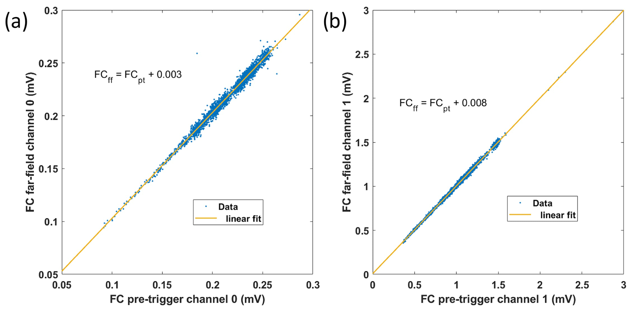
Figure 5Verification of the linear behaviour of the relationship between the background sky radiance (FC) computed for the pre-trigger (FCpt) and far field (beyond 8 km in horizontal distance, FCff) for (a) the parallel and (b) the perpendicular channels. The example presented is from flight F03 on 26 January 2020.
5.2 Level 1.5
5.2.1 Description
To build Level 1.5 data, the raw sampling along the line of sight has been degraded in order to ensure the independence of each point on the horizontal lidar profile. The final resolution is then 15 m. The ALiAS-derived Level 1.5 data are then profiles corrected from both geometric factor and solid angle of detection. They are also corrected for molecular transmission via the molecular optical thickness τm to produce the apparent backscatter coefficient (ABC, also referred to as attenuated backscatter coefficient) which is expressed as
An example of the ABC for the flight on 28 January 2020 is given in Fig. 6. The ABC decreases away from the plane because of attenuation by aerosols and clouds (passing from orange to green in Fig. 6a). In parallel with the ABC profiles, the volume depolarization ratio (VDR) is calculated from the two polarized lidar channels according to a procedure explained in Chazette et al. (2012a, b). The relationships are recalled below. They take into account the transmissions of the parallel polarization of the two Brewster plates used: for channel 0 ( and for channel 1 (. The signals on the two lidar channels contain a contribution of the complementary polarization. The VDR is then expressed as a function of the ratio of the gains Rc of the two channels.
with
The molecular volume depolarization ratio VDRm is equal to 0.3945 % at 355 nm (Collis and Russel, 1976). The term measures how the lidar system is affected by imperfect separation of polarizations. The laser residual cross-polarization of 0.002 can be neglected for ALiAS. The calibration of the depolarization consists in estimating Rc from measurements in a molecular atmosphere, above any aerosol layer. The flight of 25 January around Barbados was dedicated to this calibration with an excursion of the aircraft above 4.5 km a.m.s.l. The calibration obtained is shown in Fig. 7a. The variability of Rc is less than 2 %, which leads to an absolute error on the VDR of the order of 0.2 %. It is verified a posteriori that there is little aerosol at the calibration altitude, as shown (Fig. 7b) by the vertical profile of the aerosol extinction coefficient for the flight considered (see Sect. 5.3).
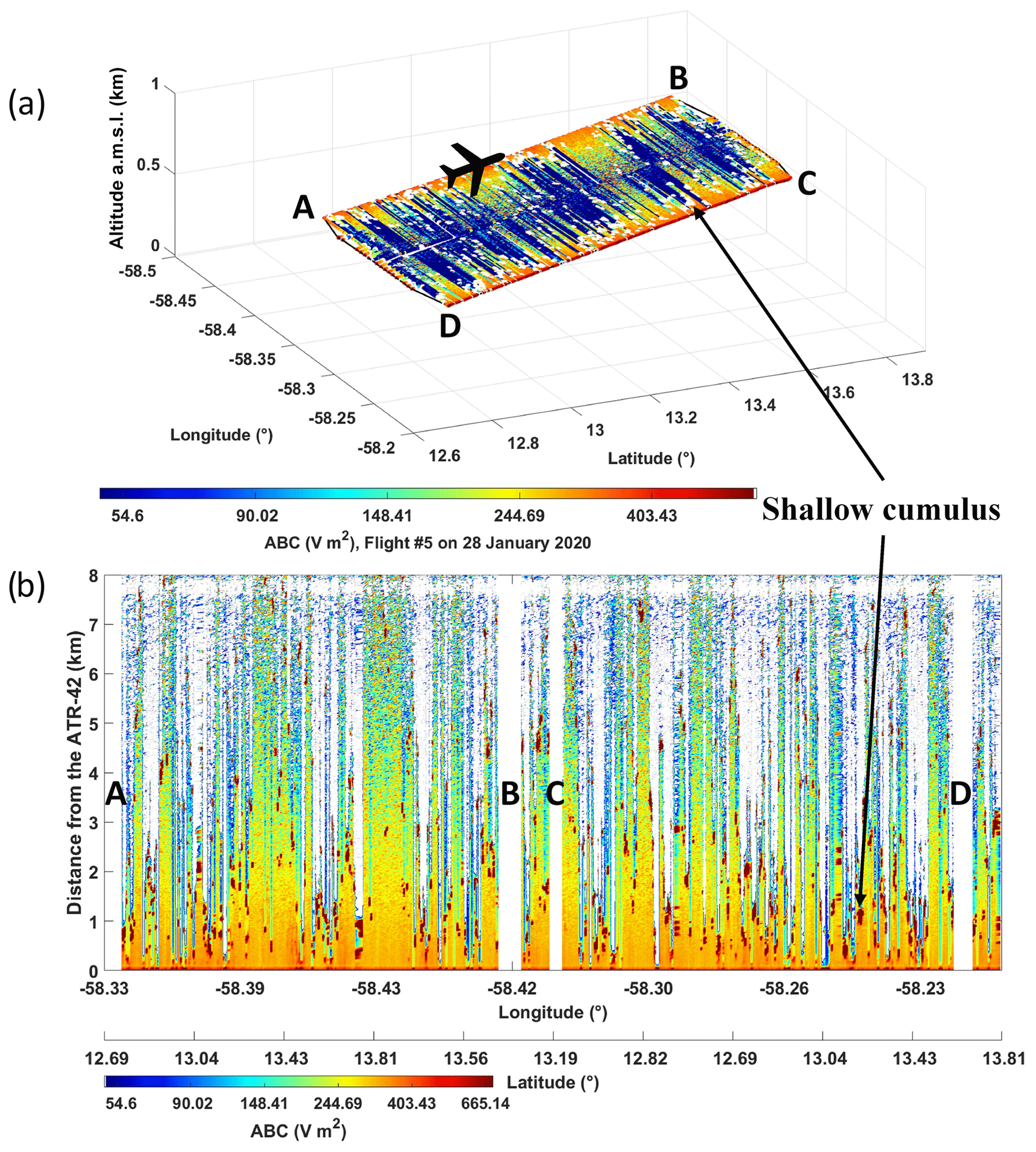
Figure 6Example of the apparent backscatter coefficient (ABC) for the flight F05 on 28 January 2020, for the first rectangle of Phase 2. The lidar data in (a) are presented as a nearly horizontal map of ABC (with each data point being geo-localized in space as a function of latitude, longitude and altitude) which is used to identify the clouds within the rectangle ABCD described by the ATR-42. Panel (b) shows the same data as a function of longitude and distance from the aircraft. The clouds are colour-coded in white in (a) and brown in (b).
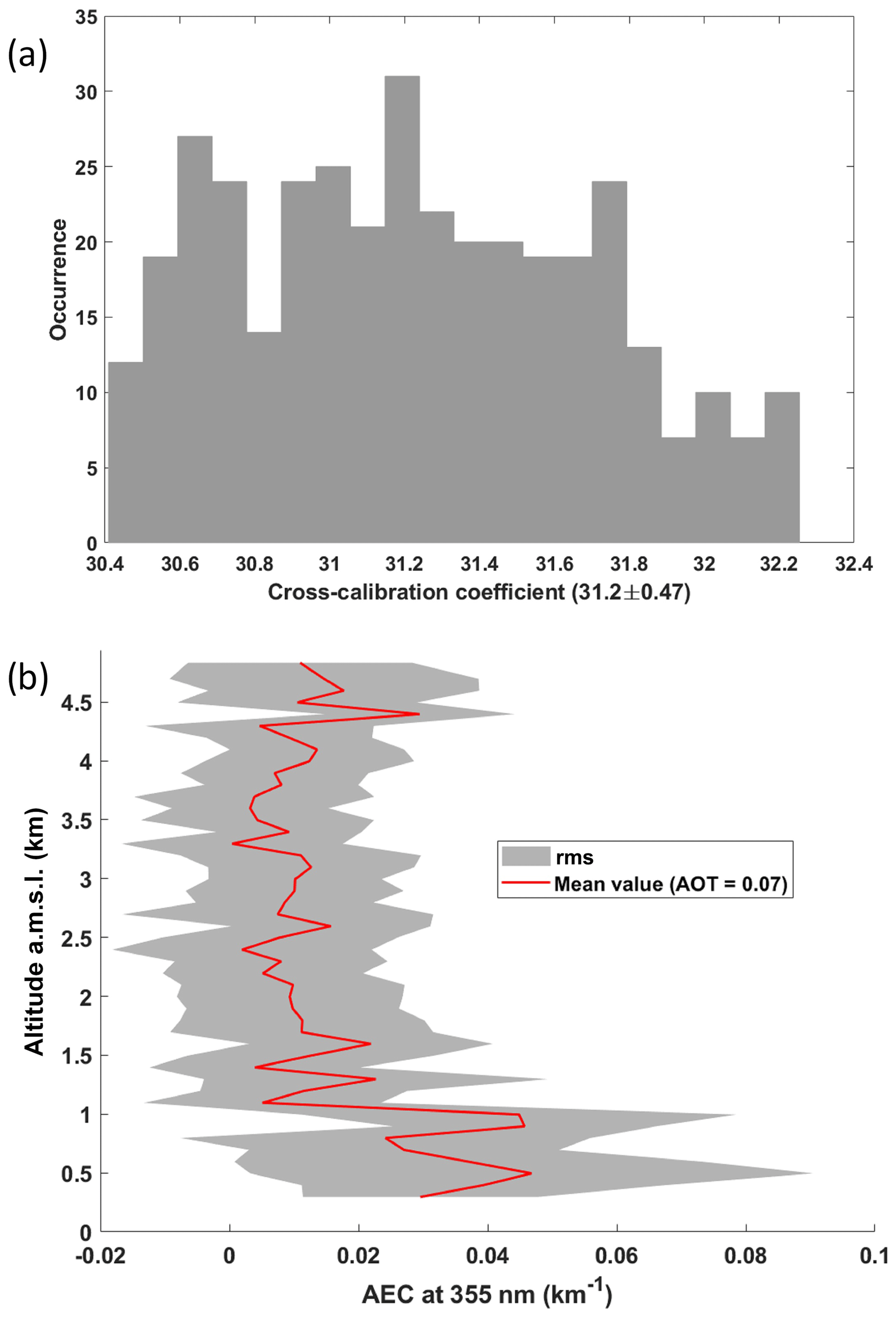
Figure 7(a) Calibration coefficient Rc of the volume depolarization ratio (VDR) derived from flight altitude above 4.5 km on 25 January 2020 (flight F04). (b) Vertical profile of the average aerosol extinction coefficient (AEC) with its root-mean-square variability (RMS) for the flight range on 25 January 2020. It corresponds to the Level 3 aerosol product. The aerosol optical thickness (AOT) is also reported.
5.2.2 Overlap factor
The overlap factor corresponds to the overlap between the laser beam and the field of view of the telescope. It is equal to 1 when the two fields completely overlap and leads to a geometric attenuation of the lidar when the overlap is partial. It can be computed from horizontal shots as previously performed for ALiAS during flights with an ultralight aircraft (Chazette et al., 2018). This calculation requires an homogeneous atmosphere along the line of sight of the lidar over a distance of about 1.5 km from the aircraft. To ensure this homogeneity, we performed the calibration at high altitude during the flight of 25 January 2020, above 4.5 km a.m.s.l., where the scattering is essentially molecular. The overlap factor of the two ALiAS channels is given in Fig. 8. It is similar for both channels beyond 300 m distance from the emission. Compared to the theoretical overlap factor due to purely geometric effects, it shows a slight bump which is related to a non-zero angle of incidence on the interference filters of the lidar, for rays coming from the far field. This small deviation is nevertheless corrected for Level 2 and Level 3 processing.

5.3 Level 2 and Level 3
Level 2 data are products provided for each individual lidar profile, for both cloud detection and calculation of the aerosol extinction coefficient (AEC) along the horizontal line of sight. Level 3 data result from statistics on Level 2 data.
5.3.1 Cloud products
Description of Level 2 cloud products
Cloud detection is applied to the lidar data acquired during Phase 2 of the flights (rectangles). It is the basis of the Level 2 cloud dataset. For each lidar ABC profile, it uses a threshold approach as already considered for lidar measurements at nadir (Chazette et al., 2001; Shang and Chazette, 2014). The threshold is proportional to the standard deviation of the noise of the cloud-free signal during Phase 2 of a given flight. Although the coefficient of proportionality Ce is constant, the threshold varies with the distance from the aircraft owing to the decrease in the signal-to-noise ratio (due to the increase in the clear-sky noise) away from the aircraft. As for the aerosol products, a lidar profile is considered to be cloud-free if the logarithm of the ABC can be considered linear with a relative error of less than 10 % (see Sect. 5.3.2). The threshold is then calculated at a constant altitude (around the cloud base height, where molecular and particle scattering can be considered constant) and when the angle of the lidar line of sight with the horizontal does not exceed 3∘ (the mean value is 1∘ and the standard deviation is 0.5∘). Lidar profiles acquired during ATR-42 turns are therefore excluded from the cloud Level 2 data. Figure 9a shows the evolution of the cloud-free lidar signal averaged over Phase 2 and the associated standard deviation along the horizontal line of sight for flight F05 on 28 January 2020. The standard deviation increases very rapidly with distance, just as the ABC decreases. The cloud detection was tested for different values of the coefficient Ce ranging from 1 to 8. The cloud mask turned out to be fairly insensitive to the value of Ce as long as Ce ranges from 2 and 4. To construct the Level 2 data, we choose Ce = 2.5.
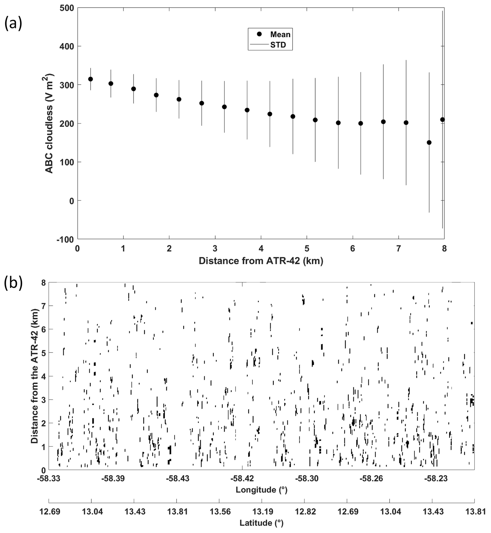
Figure 9(a) Average apparent backscatter coefficient (ABC) per 500 m distance range for all cloud-free profiles of Phase 2 for the flight F05 on 28 January 2020. The standard deviation (STD) is also reported. (b) Binary cloud detection matrix derived from ALiAS measurements along the horizontal line of slight for the flight F05 on 28 January 2020, for the first rectangle of Phase 2. The cloud mask is based on a cloud detection that uses Ce = 2.5, D=30 m and Lmin = 45 m. It is part of Level 2 cloud products.
Figure 9b shows that the cloud density decreases with the distance from the aircraft, especially beyond 3–4 km. This results from two different effects: as the distance from the aircraft increases, (1) the threshold for cloud detection increases (mostly because the magnitude of the noise increases; see Fig. 9a), and (2) the probability for the laser beam to be attenuated increases if multiple clouds are present along the laser line of sight. In general, one can be confident in the detection of semi-transparent cloud layers over the first 3–4 km. Beyond that, cloud detection is still possible, especially when there are no significant scattering layers (such as a dense aerosol plume) between the laser source and the cloud, but with a higher uncertainty on the detection of the cloud edges and thus the cloud depth. The presence of dense clouds that cannot be traversed by the laser beam will lead to an underestimate of the cloud cover and a negative bias on the average cloud depth. At cloud base, such clouds were only present on a few days during the campaign (e.g. F07, F12, F17, F18 and F19).
Two additional parameters are considered for the cloud detection that can potentially be adjusted. First, we consider that two cloudy points separated by clear sky correspond to two distinct clouds only if they are separated by a distance of at least D (in other terms, two cloudy points separated by clear sky but less than D apart will be considered to be part of the same cloud). Recognizing that trade-wind cumuli can be very small and close to each other (e.g. Zhao and Di Girolamo, 2007), we chose D=30 m. Second, to avoid interpreting as a cloud a peak of the signal that would arise from noise, we impose that a cloud corresponds to a segment of adjacent cloudy points (along the line of sight) longer than a certain threshold referred to as Lmin. The width Lmin is more difficult to estimate. We use Lmin=45 m to eliminate isolated peaks (one to two points only) of the lidar profiles that result from noise and strongly influence the statistics of cloud detection beyond 3–4 km. The two parameters D and Lmin are tuneable, and the points of the cloud mask affected by these parameters are flagged in a quality indicator.
Level 2 products also include the distance d0 beyond which the lidar signal (ABC) can be considered undistinguishable from noise (10 consecutive points within noise after the last cloud point detected). This distance is located in a non-cloudy part of the horizontal lidar profile. It is worth noting that the ABC of clouds is more than an order of magnitude greater than that of clear air and that the lidar signal can be in the noise at d0 while still showing the presence of a cloud at a greater distance.
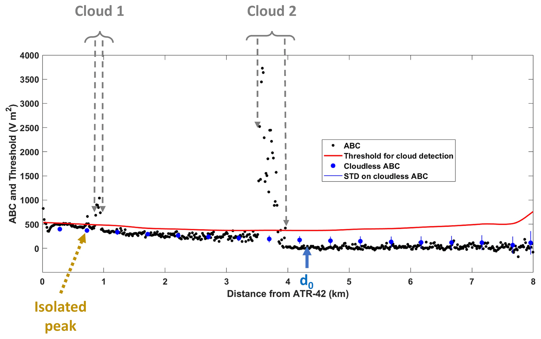
Figure 10Illustration of the cloud detection procedure on the apparent backscatter coefficient (ABC) during flight F11 on 5 February 2020 (10:13:29). Two clouds are detected that correspond to successive points for which the ABC exceeds the ABC threshold (in red). An isolated peak is not considered to be a cloudy point. The distance d0 at which the ABC can be considered to be embedded in the noise is reported. The blue dotted line is the cloud-free ABC for Phase 2 of flight F11. The standard deviation of the cloud-free ABC is also reported (blue vertical bars). At each distance, the threshold for cloud detection is defined as Ce times the threshold value.
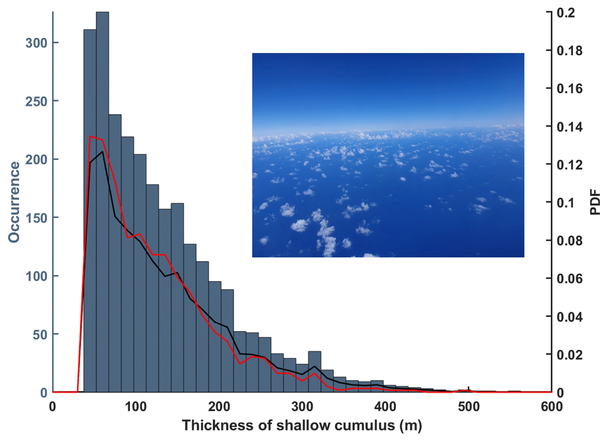
Figure 11Number of clouds detected along the horizontal line of sight of the lidar that correspond to different cloud widths during Phase 2 of flight F05 on 28 January 2020 (Level 3 cloud product). Also reported (right-hand-side vertical axis) is the probability distribution function of cloud widths for the clouds detected at horizontal distances from the aircraft ranging from 0.1 to 8 km (black solid line) and from 3 to 8 km (red solid line). The picture illustrates the type of cloud field sampled during this flight.
Figure 11 shows an example of the detection of cloud structures on one of the lidar profiles of flight F11 (2020-02-05 10:13:29). Two clouds are detected at a distance of about 0.9 and 3.8 km from the ATR-42. They correspond to segments composed of at least three successive points for which the ABC exceeds the threshold value. On the other hand, despite their ABC larger than the threshold, the segments shorter than Lmin or the “isolated peaks” are not considered to be cloudy points. The distance d0 is reported around 4.2 km.
Description of Level 3 cloud products
Level 3 cloud products consist of probability distribution functions (PDFs) of cloud chords along the laser line of slight computed during Phase 2 of the flight. It is worth noting that owing to the integration and acquisition time of the lidar measurement (5 s) and the aircraft speed (100 ms−1), we are unable to derive a cloud mask along the direction of aircraft motion (the minimum distance we can resolve along this direction is 500 m, which is roughly the upper bound of the cloud chords measured along the line of sight of the lidar). The cloud mask distributed in the Level 2 and Level 3 datasets thus corresponds to the cloud detection done along the line of sight of the lidar only. If clouds were homogeneously distributed within the field of view of the lidar, and perfectly detected by the lidar, similar PDFs would be inferred whatever the distance from the aircraft. Figure 11 shows the cloud width histogram derived at cloud base during flight F05 on 28 January 2020. The distribution obtained for the whole field of view of the lidar (clouds detected for horizontal distances between 0.1 and 8 km) is compared to the distribution obtained for clouds detected between 3 and 8 km from the aircraft. The good match of the two PDFs shows that, from a statistical point of view, the cloud detection is not biased with the distance from the aircraft, at least for cumulus cloud fields composed of optically thin clouds (also referred to as “sugar” patterns; Stevens et al., 2020). In the case of flight F05, the mean cloud width is about 130 m with a standard deviation of 80 m.
The cloud detection quality indicator/flag
Level 2 cloud product also includes a binary quality indicator (or flag) coded with “1” and “0” over 6 bits, denoted Qflag. This indicator is defined in Table 4. It takes into account for each range gate along the lidar line of sight (i) the detection or not of a cloud (bit 1); (ii) the aggregation or not of nearby cloud structures separated by less than D=30 m (bit 2); (iii) the detection of narrow cloud structures (cloud width along the line of sight < Lmin=45 m), which can be considered signal noise and which are not considered as clouds (bit 3); (iv) the vertical positioning with respect to the horizontal (Δz) of the cloud point, which depends on the angle between the line of slight and the horizontal (bits 4 and 5); and (v) visual information on the level of soiling on the external face of the aircraft window crossed by the laser beam. In order to simplify its re-reading by users, the indicator is converted into real numbers in Level 2 files. Before being used, it must be converted back to binary. For example, the real number 52 corresponds to the binary number “110100”.
Table 4Cloud detection quality indicator (Qflag) defined on 6 bits.

5.3.2 Aerosol products
The AECs are the second Level 2 and 3 products derived from the horizontal line of sight of the ALiAS lidar. The Barbados area is a region where a very wide variety of aerosols can be found. The main ones are marine aerosols to which can be added terrigenous aerosols and even biomass burning aerosols. It has been known for decades that these terrigenous aerosols mainly originate from West Africa and that their concentration over Barbados is marked by a strong seasonality (Prospero, 1968) with a maximum during the boreal summer. Dust aerosols are carried across the North Atlantic by trade winds (Trapp et al., 2010) and their concentration depends on the meteorological conditions over both Africa and the tropical North Atlantic Ocean. Main studies on desert dust aerosols have been conducted on the basis of dust events in Barbados whose sources were located more than 5000 km away over the western Sahara (e.g. Haarig et al., 2017; Trapp et al., 2010). Although this type of event occurs rarely in winter, during several flights, we observed strong AEC values associated with a significant depolarization signature. Terrigenous aerosols were actually observed for about half of the ATR flights during EUREC4A (Table 5).
The process for determining the AEC from horizontal lidar measurements was first described in Chazette et al. (2007). The horizontal configuration allows the direct measurement of the AEC, by measuring the exponential attenuation of the signal, provided the atmosphere is sufficiently homogeneous over a few kilometres, i.e. in clear-sky air (αn(z)=0). Under the conditions of the field experiment, in order to limit the effect of both the signal noise and the overlap factor, the calculation of the AEC is performed by linear regression on Ln(ABC(x,z)) in the range from 0.2 to 1 km away from the aircraft. The slope of the regression line is equal to −2αa(z) and is given by (Chazette, 2020)
Only AECs associated with a relative regression error of less than 10 % are retained. This avoids cloud-contaminated profiles in the regression range. The determination of the AEC is direct, without any hypothesis on the nature of the aerosol. In order to limit the effect related to a deviation from the horizontal, profiles with angles to the horizontal greater than 10∘ are removed. It should be noted that an angular deviation of 15∘ induces an error of 0.01 km−1 on the AEC. The mean VDR ( is also calculated over the same distance range as the AEC and is part of the aerosol Level 2 data.
Level 3 aerosol data consist of average AEC and VDR profiles calculated over each entire flight. Standard deviations on the AEC and VDR are associated with them. It was chosen to discretize the atmosphere with altitude steps of 100 m for these mean profiles.
Figure 12 shows the evolution of the AEC and VDR over the entire flight F07 on 31 January 2020 (Level 2 products). The aerosol loading is significant during Phase 2 of the flight, where cloud detection is performed. AECs of ∼ 0.3 km−1 and even higher are observed. These values should be compared to the background values which are well below 0.1 km−1. VDRs are also high, above 2 %, which is the signature of terrigenous particles in the atmosphere (e.g. Flamant et al., 2018).
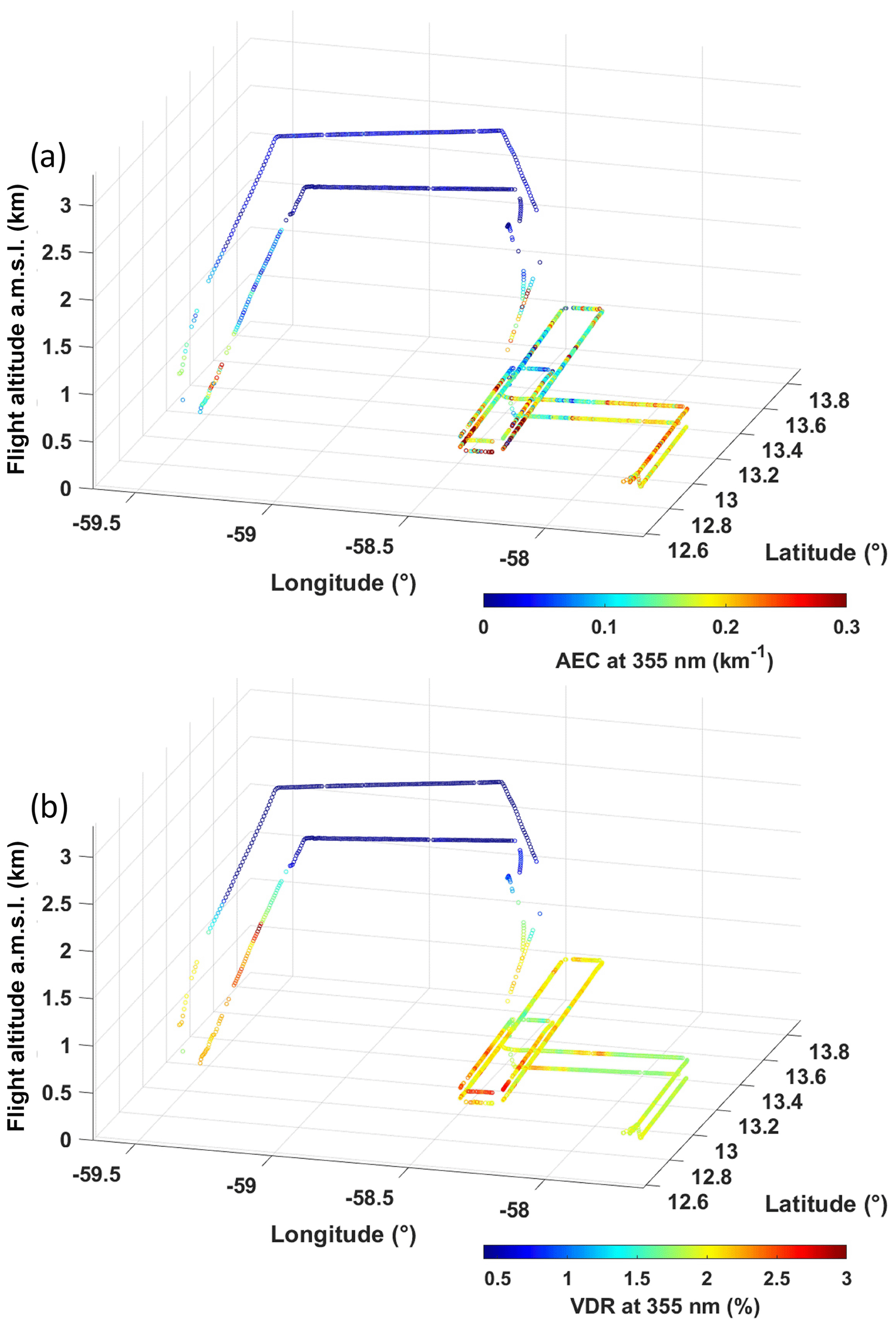
Figure 12Aerosol optical properties derived from ALiAS measurements along the horizontal line of slight on 31 January 2020 (flight F07): (a) aerosol extinction coefficient (AEC) and (b) volume depolarization ratio (VDR) which correspond to Level 2 aerosol products.
6.1 Overview of available data
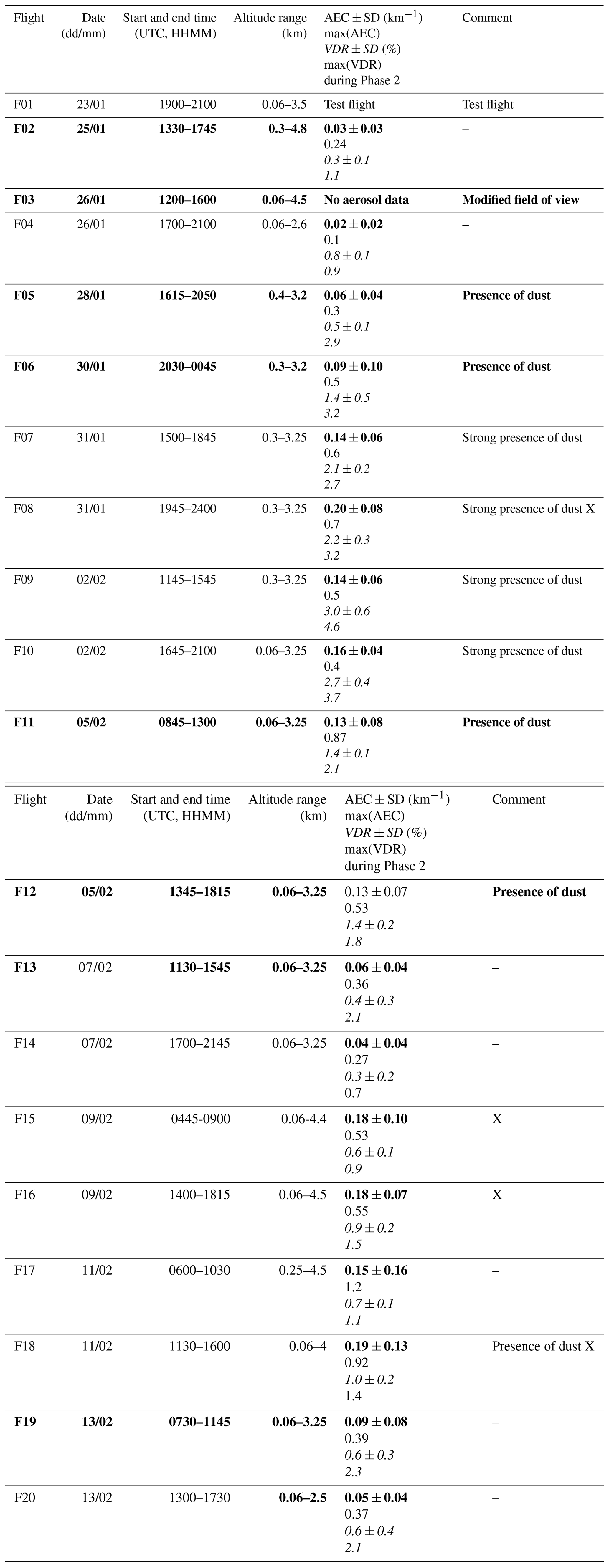
The ALiAS system has been successfully operated during the 20 flights of the EUREC4A field campaign from 23 January to 13 February 2020. The related dataset is summarized in Table 5. Flights where the lidar sampled a significant number of clouds (1000) are highlighted in bold font. The mean value of the AEC and its standard deviation informs on the amount of aerosols encountered during Phase 2 of each flight (Fig. 3). Note that Phase 2 was not carried out during the test flight on 23 January 2020.
Table 5General flight characteristics of ATR-42 when operating ALiAS. The mean, standard deviation and maximum value of the aerosol extinction coefficient (AEC) and the volume depolarization ratio (VDR) for each Phase 2 (Fig. 3) of each flight are reported. The flights in bold font are those associated with the detection of many clouds. The italic font is used for values of the VDR. The comment “Strong presence of dusts” corresponds to VDR > 2 % and the comment “Presence of dusts” corresponds to 1 % < VDR < 2 %. Flights with a reduced detection range due to window clogging by dusts and/or sea salt aerosols are indicated by “X”.
6.2 Files format
For each flight, data are available within the database as NetCDF files (version 4) for the four levels of processing described in Sect. 5. The Level 1 NetCDF file contains raw data recorded during the whole duration of the flight. It contains all the scalar and time-dependent parameters needed to properly process the signal recorded by each lidar channel. The Level 1.5 NetCDF file contains pre-processed lidar profiles of ABC and VDR along the lidar line of sight, as a function of time. Also provided are the distance from the aircraft (time dependent) and flight attitude, localization, and altitude useful for data geo-localization.
Level 2 and Level 3 are concatenated into one single NetCDF file, separately for cloud and aerosol products. The aerosol Level 2 and 3 NetCDF file contains cloud-free AEC individual values with the corresponding altitude, time and geo-localization parameters and the mean vertical profile of AEC within the altitude range of the flight, respectively. The cloud Level 2 and 3 NetCDF file contains the ABC used in the detection algorithm of clouds, a binary cloud detection array (cloud mask) and a quality flag array. All-three are given as a function of the distance from the aircraft and are restricted to the rectangle flight patterns of Phase 2 and profiles with roll–pitch angles close to 0∘. The Level 2 and 3 NetCDF file also includes the probability density functions (PDFs) of the cloud widths encountered during Phase 2 of the flight. PDFs are computed along the horizontal lines of sight for distances ranging between 0.1 and 8 km, and between 3 and 8 km, to check for the consistency of measurements in the near and far fields.
The entire dataset is published open access on the AERIS database (https://en.aeris-data.fr/, last access: 12 November 2020). The digital object identifier (DOI) for Level 1 and Level 1.5 data is https://doi.org/10.25326/57 (Chazette et al., 2020c). For Level 2 and 3 data, it is https://doi.org/10.25326/58 for the cloud products (Chazette et al., 2020b) and https://doi.org/10.25326/59 for the aerosol products (Chazette et al., 2020a). The typical sizes of the different NetCDF files are (i) ∼ 195–420 Mb for Level 1 data, (ii) ∼ 11–29 Mb for Level 1.5 data, (iii) ∼ 4–18 Mb for Level 2&3 cloud products and (iv) ∼ 60–190 Kb for Level 2&3 aerosol products.
An airborne sidewards-staring lidar was implemented on board the ATR-42 for the EUREC4A field campaign. Twenty flights were conducted from 23 January to 13 February 2020 over the west Atlantic Ocean tropical region, off the coast of Barbados. The horizontal line of sight of the lidar allowed us to characterize horizontal fields of shallow cumuli with a much better sampling than would have been the case with nadir or zenith measurements. This new dataset will make it possible to analyse the macroscopic properties of shallow cumuli near cloud base for a range of meteorological conditions and mesoscale organizations. It will also offer a baseline measurement to assess the value of future space-borne missions as the forthcoming Earth Clouds, Aerosols and Radiation Explorer mission (EarthCARE; Illingworth et al., 2015) and to evaluate the realism of the new-generation climate models. Aerosol optical parameters were also derived; biomass burning and dust aerosol plumes were present during the field campaign. The data have been classified according to the level of numerical processing applied: (i) Level 1 data are the raw horizontal lidar profiles, (ii) Level 1.5 data are the calibrated lidar profiles corrected from system characteristics, (iii) Level 2 data are the geophysical parameters directly derived from the individual profiles and (iv) Level 3 data are the synthesis of these parameters. Level 2 and Level 3 data have been combined in the same NetCDF files. All these data are available on the AERIS database (https://en.aeris-data.fr/, last access: 12 November 2020).
PC participated in the field experiment on board ATR-42; analysed the data; developed the algorithms for the Level 1.5, Level 2 and Level 3 datasets; and wrote the paper. JT, AB and CF participated in the field experiment on board ATR-42 and contributed to the paper writing. SB coordinated the project, participated in the field experiment on board ATR-42 and contributed to the paper writing.
The authors declare that they have no conflict of interest.
This article is part of the special issue “Elucidating the role of clouds–circulation coupling in climate: datasets from the 2020 (EUREC4A) field campaign”. It is not associated with a conference.
The idea of trying horizontal lidar measurements to characterize clouds at cloud base was suggested to us by Bjorn Stevens at the outset of the EUREC4A project. The authors gratefully acknowledge Jean-Christophe Canonici, Jean-Christophe Desbios, Thierry Perrin, Laurent Guiraud and all the technicians, engineers, pilots and director from SAFIRE, the French facility for airborne research (http://www.safire.fr, last access: 12 November 2020), and airplane delivery, for making the preparation of the ATR and the EUREC4A airborne operations possible. We thank the Caribbean Regional Security System (RSS) for hosting the ATR and the ATR team in Barbados during the experiment; David Farrell and the Caribbean Institute for Meteorology and Hydrology (CIMH) for their logistical and administrative support; and the Department of Civil Aviation in Barbados and Andrea Hausold (from DLR), for their help and support of airborne operations. The authors also thank AERIS for their support during the campaign and for managing the EUREC4A database. The authors are thankful to the three anonymous referees whose comments helped improve the overall quality of the paper.
The EUREC4A project was supported by the European Research Council (ERC) under the European Union’s Horizon 2020 research and innovation programme (grant agreement no. 694768), with some additional support from the French Space Agency CNES through the EECLAT proposal.
This paper was edited by Gijs de Boer and reviewed by three anonymous referees.
Berthier, S., Chazette, P., Pelon, J., and Baum, B.: Comparison of cloud statistics from spaceborne lidar systems, Atmos. Chem. Phys., 8, 6965–6977, https://doi.org/10.5194/acp-8-6965-2008, 2008.
Bony, S. and Dufresne, J. L.: Marine boundary layer clouds at the heart of tropical cloud feedback uncertainties in climate models, Geophys. Res. Lett., 32, 1–4, https://doi.org/10.1029/2005GL023851, 2005.
Bony, S., Stevens, B., Ament, F., Bigorre, S., Chazette, P., Crewell, S., Delanoë, J., Emanuel, K., Farrell, D., Flamant, C., Gross, S., Hirsch, L., Karstensen, J., Mayer, B., Nuijens, L., Ruppert, J. H., Sandu, I., Siebesma, P., Speich, S., Szczap, F., Totems, J., Vogel, R., Wendisch, M., and Wirth, M.: EUREC4A: A Field Campaign to Elucidate the Couplings Between Clouds, Convection and Circulation, Surv. Geophys., 38, 1529–1568, https://doi.org/10.1007/s10712-017-9428-0, 2017.
Bony, S., Schulz, H., Vial, J., and Stevens, B.: Sugar, Gravel, Fish, and Flowers: Dependence of Mesoscale Patterns of Trade-Wind Clouds on Environmental Conditions, Geophys. Res. Lett., 47, 1–12, https://doi.org/10.1029/2019GL085988, 2020.
Brient, F., Schneider, T., Tan, Z., Bony, S., Qu, X., and Hall, A.: Shallowness of tropical low clouds as a predictor of climate models' response to warming, Clim. Dynam., 47, 433–449, https://doi.org/10.1007/s00382-015-2846-0, 2016.
Chazette, P.: Aerosol optical properties as observed from an ultralight aircraft over the Strait of Gibraltar, Atmos. Meas. Tech., 13, 4461–4477, https://doi.org/10.5194/amt-13-4461-2020, 2020.
Chazette, P., Pelon, J., and Mégie, G.: Determination by spaceborne backscatter lidar of the structural parameters of atmospheric scattering layers., Appl. Optic, 40, 3428–3440, https://doi.org/10.1364/AO.40.003428, 2001.
Chazette, P., Sanak, J., and Dulac, F.: New approach for aerosol profiling with a lidar onboard an ultralight aircraft: application to the African Monsoon Multidisciplinary Analysis., Environ. Sci. Technol., 41, 8335–8341, https://doi.org/10.1021/es070343y, 2007.
Chazette, P., Bocquet, M., Royer, P., Winiarek, V., Raut, J. C., Labazuy, P., Gouhier, M., Lardier, M., and Cariou, J. P.: Eyjafjallajökull ash concentrations derived from both lidar and modeling, J. Geophys. Res.-Atmos., 117, D00U14, https://doi.org/10.1029/2011JD015755, 2012a.
Chazette, P., Dabas, A., Sanak, J., Lardier, M., and Royer, P.: French airborne lidar measurements for Eyjafjallajökull ash plume survey, Atmos. Chem. Phys., 12, 7059–7072, https://doi.org/10.5194/acp-12-7059-2012, 2012b.
Chazette, P., Raut, J.-C., and Totems, J.: Springtime aerosol load as observed from ground-based and airborne lidars over northern Norway, Atmos. Chem. Phys., 18, 13075–13095, https://doi.org/10.5194/acp-18-13075-2018, 2018.
Chazette, P., Totems, J., Baron, A., Flamant, C., and Bony, S.: EUREC4A – ATR-42 – Lidar ALiAS – Level 2 & 3 aerosol products, AERIS data Cent., https://doi.org/10.25326/59, 2020a.
Chazette, P., Totems, J., Baron, A., Flamant, C., and Bony, S.: EUREC4A ATR-42 Lidar ALiAS – Level 2 & 3 cloud products, AERIS data Cent., https://doi.org/10.25326/58, 2020b.
Chazette, P., Totems, J., Baron, A., Flamant, C., and Bony, S.: EUREC4A ATR-42 Lidar ALiAS – Levels 1 & 1.5, AERIS data Cent., https://doi.org/10.25326/57, 2020c.
Collis, R. T. H. and Russel, P. B.: Laser Monitoring of the Atmosphere, edited by: Hinkley, E. D., Springer Berlin Heidelberg, Berlin, Heidelberg., 1976.
Flamant, C., Deroubaix, A., Chazette, P., Brito, J., Gaetani, M., Knippertz, P., Fink, A. H., de Coetlogon, G., Menut, L., Colomb, A., Denjean, C., Meynadier, R., Rosenberg, P., Dupuy, R., Dominutti, P., Duplissy, J., Bourrianne, T., Schwarzenboeck, A., Ramonet, M., and Totems, J.: Aerosol distribution in the northern Gulf of Guinea: local anthropogenic sources, long-range transport, and the role of coastal shallow circulations, Atmos. Chem. Phys., 18, 12363–12389, https://doi.org/10.5194/acp-18-12363-2018, 2018.
Haarig, M., Ansmann, A., Althausen, D., Klepel, A., Groß, S., Freudenthaler, V., Toledano, C., Mamouri, R.-E., Farrell, D. A., Prescod, D. A., Marinou, E., Burton, S. P., Gasteiger, J., Engelmann, R., and Baars, H.: Triple-wavelength depolarization-ratio profiling of Saharan dust over Barbados during SALTRACE in 2013 and 2014, Atmos. Chem. Phys., 17, 10767–10794, https://doi.org/10.5194/acp-17-10767-2017, 2017.
Illingworth, A. J., Barker, H. W., Beljaars, A., Ceccaldi, M., Chepfer, H., Clerbaux, N., Cole, J., Delanoë, J., Domenech, C., Donovan, D. P., Fukuda, S., Hirakata, M., Hogan, R. J., Huenerbein, A., Kollias, P., Kubota, T., Nakajima, T. Y., Nakajima, T. Y., Nishizawa, T., Ohno, Y., Okamoto, H., Oki, R., Sato, K., Satoh, M., Shephard, M. W., Velázquez-Blázquez, A., Wandinger, U., Wehr, T., and Van Zadelhoff, G. J.: The earthcare satellite?: The next step forward in global measurements of clouds, aerosols, precipitation, and radiation, B. Am. Meteorol. Soc., 96, 1311–1332, https://doi.org/10.1175/BAMS-D-12-00227.1, 2015.
Johnson, B. T. T., Heese, B., McFarlane, S. A. a., Chazette, P., Jones, A., and Bellouin, N.: Vertical distribution and radiative effects of mineral dust and biomass burning aerosol over West Africa during DABEX, J. Geophys. Res., 113, 1–16, https://doi.org/10.1029/2008JD009848, 2008.
Liou, K.-N. and Schotland, R. M.: Multiple Backscattering and Depolarization from Water Clouds for a Pulsed Lidar System, J. Atmos. Sci., 28, 772–784, https://doi.org/10.1175/1520-0469(1971)028<0772:MBADFW>2.0.CO;2, 1971.
Medeiros, B., Stevens, B., and Bony, S.: Using aquaplanets to understand the robust responses of comprehensive climate models to forcing, Clim. Dynam., 44, 1957–1977, https://doi.org/10.1007/s00382-014-2138-0, 2015.
Norris, J. R.: Low cloud type over the ocean from surface observations. Part II: Geographical and seasonal variations, J. Climate, 11, 383–403, https://doi.org/10.1175/1520-0442(1998)011<0383:LCTOTO>2.0.CO;2, 1998.
Nuijens, L. and Siebesma, A. P.: Boundary Layer Clouds and Convection over Subtropical Oceans in our Current and in a Warmer Climate, Curr. Clim. Chang. Reports, 5, 80–94, https://doi.org/10.1007/s40641-019-00126-x, 2019.
Palm, S. P., Benedetti, A., and Spinhirne, J.: Validation of ECMWF global forecast model parameters using GLAS atmospheric channel measurements, Geophys. Res. Lett., 32, L22S09, https://doi.org/10.1029/2005GL023535, 2005.
Pierrehumbert, R. T.: Thermostats, radiator fins, and the local runaway greenhouse, J. Atmos. Sci., 52, 1784–1806, 1995.
Prospero, J. M.: atmospheric dust studies on Barbados, B. Am. Meteorol. Soc., 49, 645–652, https://doi.org/10.1175/1520-0477-49.6.645, 1968.
Redelsperger, J. L., Thorncroft, C. D., Diedhiou, A., Lebel, T., Parker, D. J., and Polcher, J.: African Monsoon Multidisciplinary Analysis: An international research project and field campaign, B. Am. Meteorol. Soc., 87, 1739–1746, https://doi.org/10.1175/BAMS-87-12-1739, 2006.
Shang, X. and Chazette, P.: Interest of a Full-Waveform Flown UV Lidar to Derive Forest Vertical Structures and Aboveground Carbon, Forests, 5, 1454–1480, https://doi.org/10.3390/f5061454, 2014.
Shang, X. and Chazette, P.: End-to-End Simulation for a Forest-Dedicated Full-Waveform Lidar onboard a Satellite Initialized from UV Airborne Lidar Experiments, Remote Sens., 7, 5222–5255, https://doi.org/10.3390/rs70505222, 2015.
Spark, M. and Cottis, M.: Pressure-induced optical distorsion in laser windows, Appl. Optics, 44, 787–794, 1973.
Spinhirne, J. D., Hansen, M. Z., and Caudill, L. O.: Cloud top remote sensing by airborne lidar, Appl. Optics, 21, 1564, https://doi.org/10.1364/ao.21.001564, 1982.
Spinhirne, J. D., Palm, S. P., Hlavka, D. L., Hart, W. D., and Welton, E. J.: Global aerosol distribution from the GLAS polar orbiting lidar instrument, IEEE Work. Remote Sens. Atmos. Aerosols, Tucson, AZ, USA, 2–8, https://doi.org/10.1109/AERSOL.2005.1494140, 2005.
Stevens, B., Ament, F., Bony, S., Crewell, S., Ewald, F., Gross, S., Hansen, A., Hirsch, L., Jacob, M., Kölling, T., Konow, H., Mayer, B., Wendisch, M., Wirth, M., Wolf, K., Bakan, S., Bauer-Pfundstein, M., Brueck, M., Delanoë, J., Ehrlich, A., Farrell, D., Forde, M., Gödde, F., Grob, H., Hagen, M., Jäkel, E., Jansen, F., Klepp, C., Klingebiel, M., Mech, M., Peters, G., Rapp, M., Wing, A. A., and Zinner, T.: A high-altitude long-range aircraft configured as a cloud observatory the narval expeditions, B. Am. Meteorol. Soc., 100, 1061–1077, https://doi.org/10.1175/BAMS-D-18-0198.1, 2019.
Stevens, B., Bony, S., Brogniez, H., Hentgen, L., Hohenegger, C., Kiemle, C., L'Ecuyer, T. S., Naumann, A. K., Schulz, H., Siebesma, P. A., Vial, J., Winker, D. M., and Zuidema, P.: Sugar, gravel, fish and flowers: Mesoscale cloud patterns in the trade winds, Q. J. Roy. Meteor. Soc., 146, 141–152, https://doi.org/10.1002/qj.3662, 2020.
Trapp, J. M., Millero, F. J., and Prospero, J. M.: Temporal variability of the elemental composition of African dust measured in trade wind aerosols at Barbados and Miami, Mar. Chem., 120, 71–82, https://doi.org/10.1016/j.marchem.2008.10.004, 2010.
Vial, J., Bony, S., Stevens, B., and Vogel, R.: Mechanisms and Model Diversity of Trade-Wind Shallow Cumulus Cloud Feedbacks: A Review, Springer, Cham, 159–181, 2017.
Winker, D. M., Pelon, J., Mccormick, M. P., Pierre, U., and Jussieu, P.: The CALIPSO mission?: Spaceborne lidar for observation of aerosols and clouds, Proc. SPIE, 4893, 1–11, https://doi.org/10.1117/12.466539, 2003.
Yorks, J. E., McGill, M. J., Palm, S. P., Hlavka, D. L., Selmer, P. A., Nowottnick, E. P., Vaughan, M. A., Rodier, S. D., and Hart, W. D.: An overview of the CATS level 1 processing algorithms and data products, Geophys. Res. Lett., 43, 4632–4639, https://doi.org/10.1002/2016GL068006, 2016.
Zhao, G. and Di Girolamo, L.: Statistics on the macrophysical properties of trade wind cumuli over the tropical western Atlantic, J. Geophys. Res.-Atmos., 112, D10204, https://doi.org/10.1029/2006JD007371, 2007.