Bed topography of Princess Elizabeth Land in East Antarctica

We present a topographic digital elevation model (DEM) for Princess Elizabeth Land (PEL), East Antarctica. The DEM covers an area of ∼900 000 km² and was built from radio-echo sounding data collected during four campaigns since 2015. Previously, to generate the Bedmap2 topographic product, PEL's bed was characterized from low-resolution satellite gravity data across an otherwise large (>200 km wide) data-free zone. We use the mass conservation (MC) method to produce an ice thickness grid across faster flowing (>30 m yr⁻¹) regions of the ice sheet and streamline diffusion in slower flowing areas. The resulting ice thickness model is integrated with an ice surface model to build the bed DEM. Together with BedMachine Antarctica and Bedmap2, this new bed DEM completes the first-order measurement of subglacial continental Antarctica – an international mission that began around 70 years ago. The ice thickness data and bed DEMs of PEL (resolved horizontally at 500 m relative to ice surface elevations obtained from the Reference Elevation Model of Antarctica – REMA) are accessible from https://doi.org/10.5281/zenodo.4023343 (Cui et al., 2020a) and https://doi.org/10.5281/zenodo.4023393 (Cui et al., 2020b).

1 Introduction

Radio-echo sounding (RES) is commonly used to measure ice thickness and to understand subglacial topography and basal ice sheet conditions (Dowdeswell and Evans, 2004; Bingham and Siegert, 2007). A series of airborne geophysical explorations were conducted across East Antarctica in the 1970s (Robin et al., 1977; Dean et al., 2008; Turchetti et al., 2008; Naylor et al., 2008), which led to the first compilation folio of maps of subglacial bed topography, ice sheet surface elevation, and ice thickness in Antarctica (Drewry and Meldrum, 1978; Drewry et al., 1980; Jankowski and Drewry, 1981; Drewry, 1983). Since then, multiple efforts have been made to collect and compile RES data in order to expand the subglacial topographic database across the continent (Lythe et al., 2001; Fretwell et al., 2013).

Geophysical surveys of the coast of Princess Elizabeth Land (PEL) began in 1971, providing basic ice thickness, bed topography, and magnetic field data (Popov and Kiselev, 2018; Popov, 2020). Prior to our work, virtually no RES data had been acquired upstream of ∼300 km from the grounding line of PEL, however. Hence, this region has been described as one of the so-called “poles of ignorance” (Fretwell et al., 2013), and its representation in recent bed DEMs (e.g., Bedmap2 and BedMachine Antarctica) is as a zone of flat topography, reflecting the absence of data (Morlighem et al., 2020). Other data gaps (Recovery Glacier system; Diez et al., 2019; South Pole; Jordan et al., 2018) have been filled recently, leaving PEL as the last remaining significant region in Antarctica to be surveyed systematically.

Figure 1 Maps of (a) ice flow velocity version 2 (Rignot et al., 2017b) and (b) the MODIS Mosaic of Antarctica (2008–2009) satellite image (Haran et al., 2014). The black line denotes the grid boundary for ICECAP2 bed elevation model. The white box indicates the location of a previously discovered elongated and extensive smooth surface, interpreted as a potential subglacial lake (Jamieson et al., 2016). (c) Geophysical flight lines from four field seasons, namely 2015–2016 (red), 2016–2017 (green), 2017–2018 (brown), and 2018–2019 (blue). The inset denotes location of the study region. Panels (b) and (c) are overlain by the MODIS Mosaic of Antarctica (2008–2009; Haran et al., 2014). The differential interferometry synthetic aperture radar (DInSAR) grounding line (yellow line) is also shown (Rignot et al., 2017a).

In the absence of bed data, glaciologists have had to rely on satellite imagery, inversion from poor-resolution satellite gravity observations, and ice flow modelling to infer the subglacial landscape and its interaction with the ice above (Fretwell et al., 2013; Jamieson et al., 2016). For example, a combination of three satellite-derived mosaics and some initial exploratory RES data (Blankenship et al., 2017) have been used to hypothesize the subglacial features of PEL, revealing the presence of a potentially large (>100 km long) subglacial lake (white box; Fig. 1a and b) and an expected canyon morphology across the PEL sector. A study by Dongchen et al. (2004) adopted interferometric synthetic aperture radar (InSAR) satellite technology to generate an experimental subglacial bed elevation model across the ice sheet margin. While the result contains a certain level of detail, it has an obvious limitation in that the bed elevation was based solely on the satellite data and without direct measurements of the subglacial landscape. Hence, the bed topography in PEL is the poorest defined of any region in Antarctica – and indeed of any land surface on Earth.

Here, we present the first detailed ice thickness DEM for PEL, based on new RES measurements collected since 2015, which we refer to as the ICECAP2 DEM. We briefly discuss the differences between the ICECAP2 DEM and its representation in both Bedmap2 and BedMachine Antarctica. The ICECAP2 bed DEM is relative to ice surface elevations from the Reference Elevation Model of Antarctica (REMA; Howat et al., 2019). The ice thickness DEM can be easily integrated with updated surface DEMs (i.e. Helm et al., 2014) and, in particular, the upcoming Bedmap3 product.

2 Study area

The PEL sector of East Antarctica is bounded on the west by the Amery Ice Shelf and on the east by Wilhelm II Land (Fig. 1). The region covered by the ICECAP2 DEM extends ∼1300 km from east to west and ∼ 800 km from north to south. We use the differential interferometry synthetic aperture radar (DInSAR) grounding line (Rignot et al., 2011) to delimit the ice-shelf-facing margin of the ice sheet. The DEM was built from recently acquired airborne geophysical data collected across PEL by the ICECAP2 programme over four austral summer seasons from 2015 to 2019 (Fig. 1c).

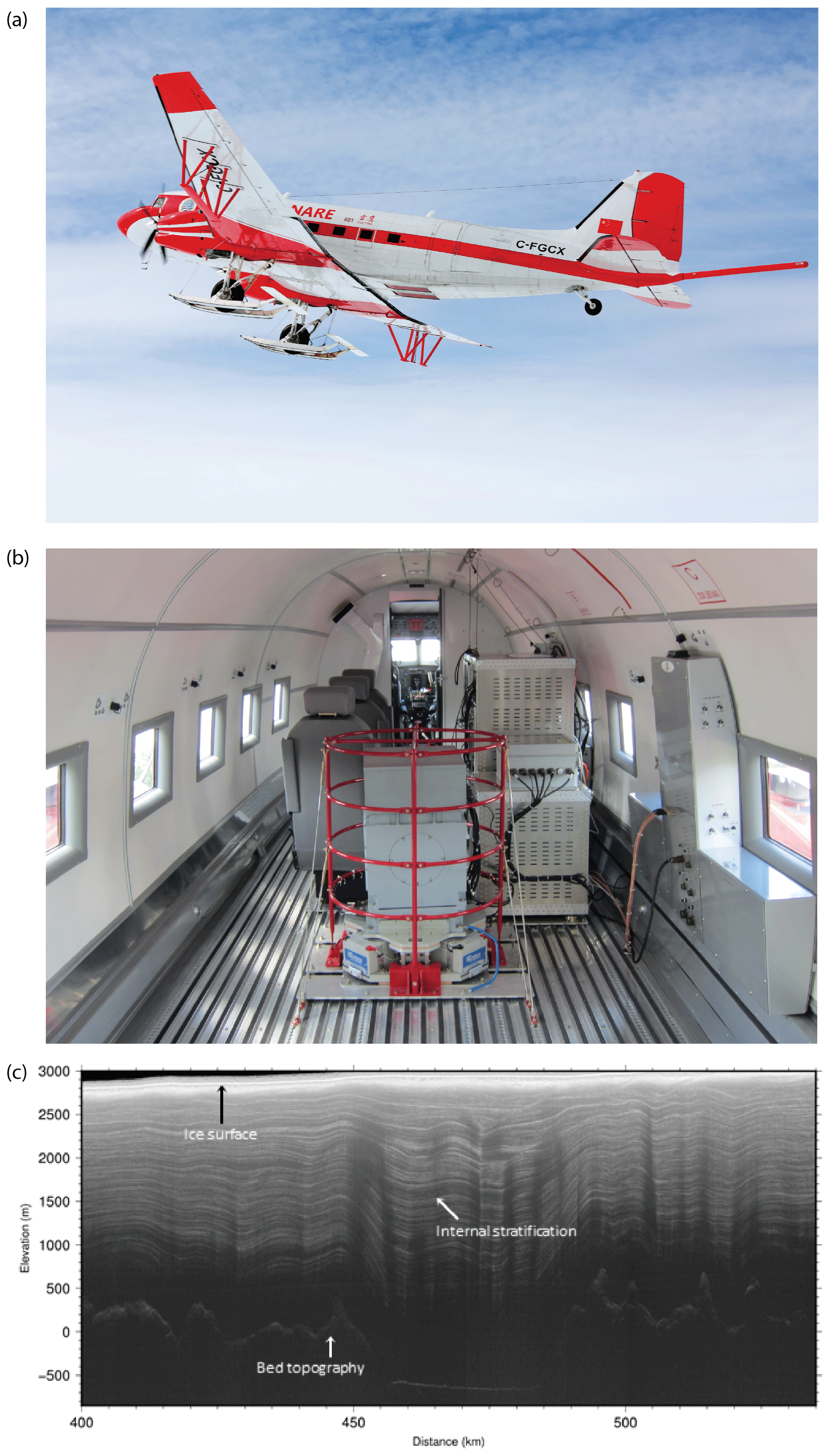
Figure 2 (a) The Snow Eagle 601 aeroplane operated by the Polar Research Institute of China for the Chinese National Antarctic Research Expedition (CHINARE) programme. (b) The interior of the aeroplane, showing the RES equipment. (c) RES data collected in 2017–2018, revealing the quality of internal layers, bed topography, and subglacial lake water between 455 and 485 km.

3 Data and methods

Field data acquisition was achieved using the Snow Eagle 601 aerogeophysical platform and a BT-67 aeroplane operated by the Polar Research Institute of China for the Chinese National Antarctic Research Expedition (CHINARE) programme (Fig. 2a and b). The suite of instruments configured on the aeroplane includes a phase-coherent RES system, functionally similar to the high-capability airborne radar sounder (HiCARS) developed by the University of Texas Institute for Geophysics (UTIG; i.e. Young et al., 2011; Greenbaum et al., 2015). HiCARS operates at a central frequency of 60 MHz and a peak power of 8 kW, making it capable of penetrating deep (>3 km) ice in Antarctica. The system has an along-track spatial sampling rate and a vertical resolution of ∼20 and ∼5.6 m, respectively. Further details on the parameters and introduction of the RES system can be found in Cui et al. (2018). A Javad GNSS Inc. GPS receiver and its four antennas were mounted at the aircraft's centre of gravity (CG), tail, and both wings. GPS data from the antenna at the aircraft's CG were used for RES data interpretation.

During the first field season (2015–2016), a survey acquiring exploratory, fan-shaped radial profiles, to maximize range and data return on each flight, was completed across the broadly unknown region of PEL. These flight lines extend from Progress Station at the coast to the interior ice sheet divide at Ridge B (Fig. 1). In the second and third seasons (2016–2017 and 2017–2018), a survey grid was completed, targeting enhanced resolution over a proposed subglacial lake and a series of basal canyons (see Jamieson et al., 2016). In the fourth season (2018–2019), a few additional transects were completed to fill the largest data gaps within aircraft range.

4 Data processing

Ice thickness measurements were derived from two RES data products from which the ice bed interface was traced and digitized, namely (a) 2D-focused synthetic aperture radar (SAR) processed data, applied to RES data from the first two seasons, and (b) unfocused field RES data from the third and fourth seasons. Raw RES data were first separated to differentiate the project/set/transect (PST) during the field data processing. Pulse compression, filtering, 10 traces coherent stacking, and five traces incoherent stacking were then applied to generate a field RES data product. The field RES data can be used for quality control and are also good enough for initial ice bed interface measurements, leading to the calculation of first-order ice thicknesses and an initial bed DEM. To achieve better quality RES images, 2D-focused SAR processing was applied to data from the first two seasons (Peters et al., 2007). The ice bed interface was picked in a semi-automatic manner, using a picking programme used previously by the ICECAP programme on data from the Aurora and Wilkes subglacial basins (Blankenship et al., 2016, 2017). Ice thicknesses were calculated by multiplying two-way travel time by the velocity of electromagnetic waves in the ice (i.e. 0.168 m ns⁻¹; Cui et al., 2018). Firn corrections were not applied and, thus, may be subject to a small systematic error. The precise point positioning method was used in the GPS processing to improve location accuracy since the flight distance is too far from the GPS base station for post-airborne GPS data processing. Processed GPS data were interpolated and fitted to the RES traces according to time stamps generated by the integrated airborne system. The aircraft to ice surface range was calculated by multiplying the two-way travel time of the RES reflections off the ice surface by the velocity in air (0.3 m ns⁻¹). Figure 2c shows examples of the RES data collected in 2017–2018.

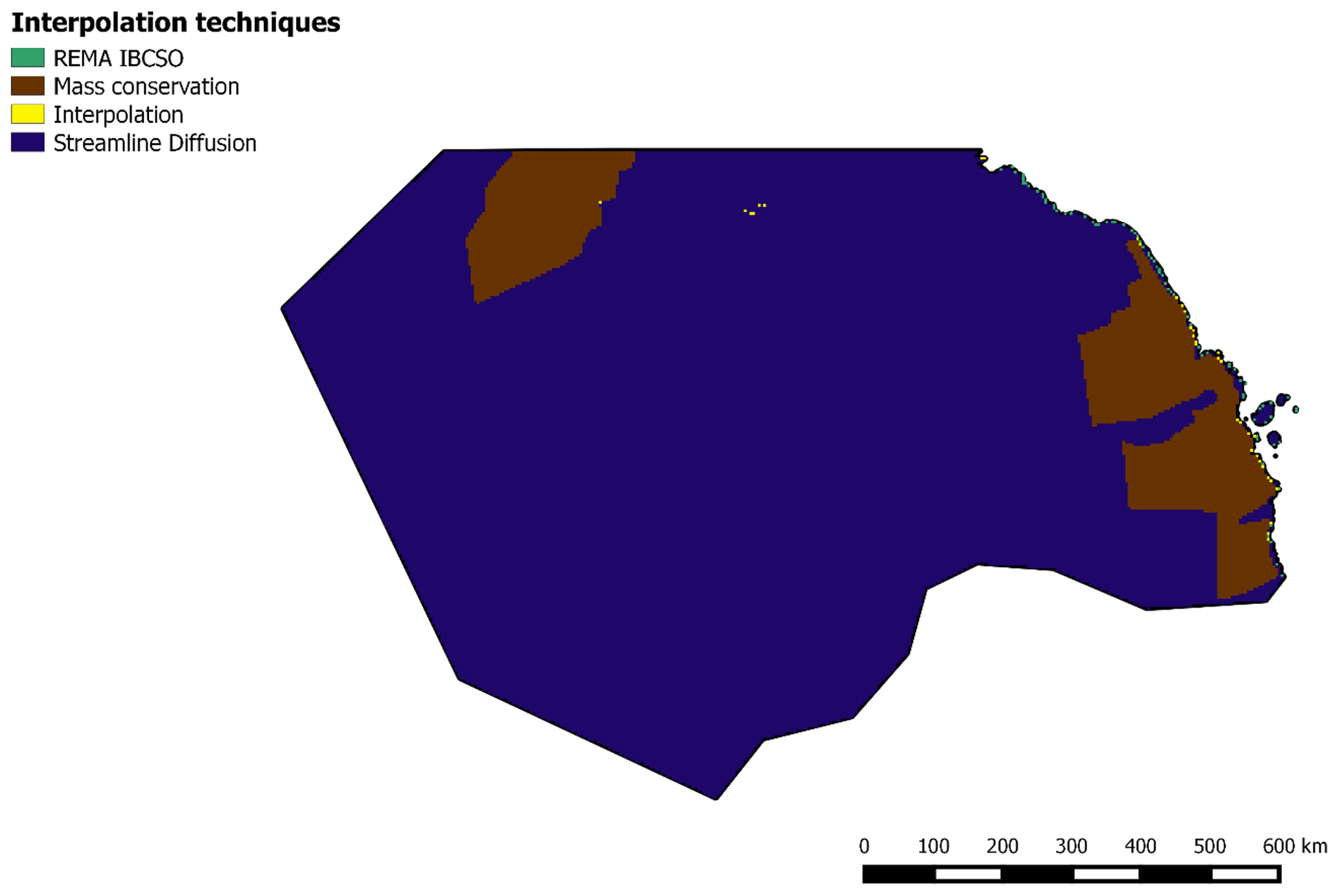
Figure 3 Map showing the interpolation techniques used to build the ice thickness DEM, including the Reference Elevation Model of Antarctica and the International Bathymetric Chart of the Southern Ocean (REMA IBCSO; green), the mass conservation (brown), the interpolation (yellow), and the streamline diffusion (blue).

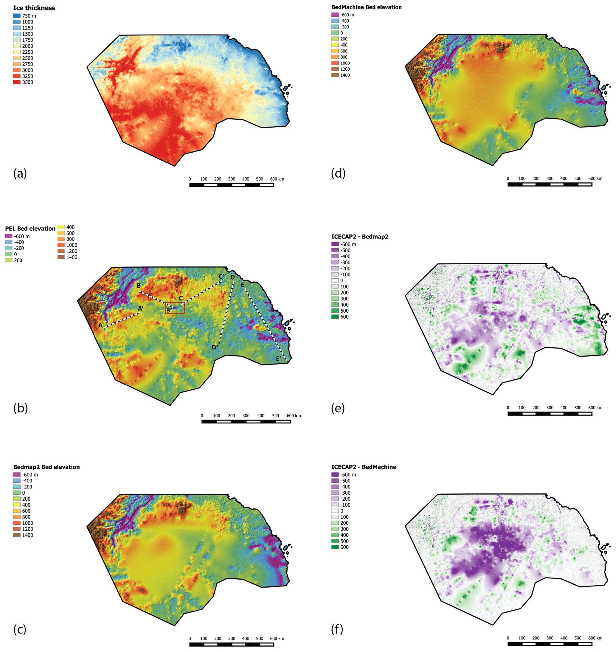
Figure 4 Bed elevation maps for Princess Elizabeth Land. (a) ICECAP2 ice thickness DEM. (b) ICECAP2 bed DEM. Profiles A–A^′, B–B^′, C–C^′, D–D^′, and E–E^′ are overlain in (b). The red box indicates the location where a large subglacial lake has been inferred (Jamieson et al., 2016). (c) Bedmap2 bed DEM. (d) BedMachine DEM. (e) Map showing the difference between the ICECAP2 and Bedmap2 DEMs. (f) Map showing the difference between the ICECAP2 and BedMachine DEMs.

To derive the ice thickness map (Fig. 4a), we employed a variety of techniques, depending on the ice speed, following the approach described in Morlighem et al. (2020). In fast-flowing regions (i.e. velocity >30 m yr⁻¹), we relied on mass conservation (MC; Fig. 3) constrained by the ICECAP2 RES data and additional RES data that were available as part of BedMachine Antarctica (Morlighem et al., 2020). In the slower moving regions inland, we relied on a streamline diffusion interpolation to fill the area between data points (Fig. 3).

For the purpose of comparing the ICECAP2 DEM (Fig. 4b) with Bedmap2 (Fig. 4c) and BedMachine Antarctica (Fig. 4d), the 500 m ice surface elevation DEM from the REMA (Howat et al., 2019) was used. Prior to the subtraction process, the Bedmap2 and BedMachine ice thickness DEMs were transformed from the g104c geoid vertical reference to the World Geodetic System (WGS) 1984 vertical reference frame. The ice thickness for both Bedmap2 and BedMachine are in ice equivalent rather than an estimate of the ice thickness from firn corrections. The Bedmap2 and BedMachine ice thickness DEMs were resampled, using the bilinear function in ArcGIS, to a 500 m spacing and referenced to the polar stereographic projection (Snyder, 1987). The ice thickness in all three models was then subtracted from the ice surface elevation DEM (Howat et al., 2019) to produce bed DEMs at a 500 m resolution. Difference maps were then computed by subtracting the Bedmap2 (Fig. 4e) and BedMachine (Fig. 4f) bed DEMs from the ICECAP2 bed DEM. Crossover analyses revealed root mean square (RMS) errors within the ICECAP2 RES data of 24.2 m (2015–2016), 39.2 m (2016–2017), 10.4 m (2017–2018), 7.5 m (2018–2019), and 35.4 m (for the full data set).

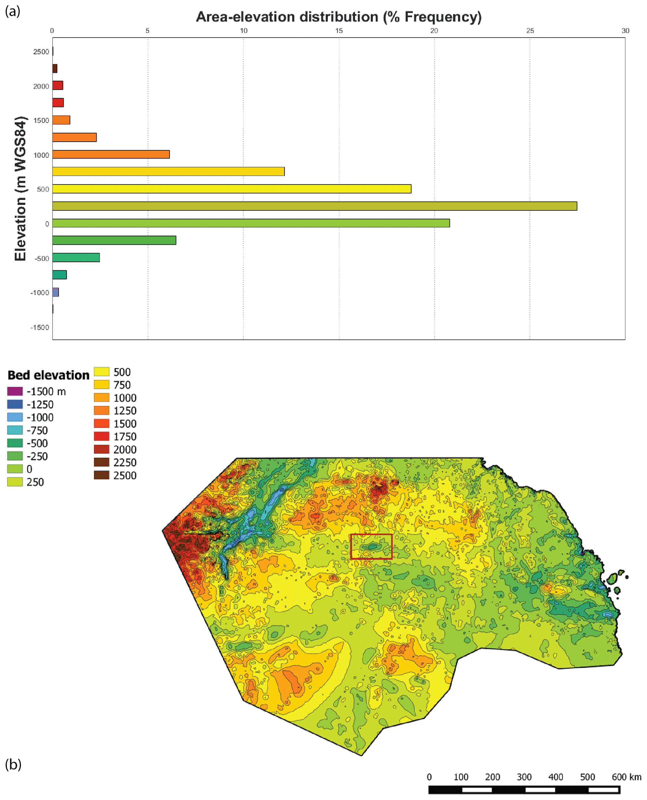
Figure 5 (a) Hypsometry (area–elevation distribution) derived from the ICECAP2 DEM. (b) ICECAP2 DEM in the same elevation-related colour scheme as (a).

5 Results

5.1 Subglacial morphology of Princess Elizabeth Land

The ICECAP2 RES data allow us to form an appreciation of the subglacial topography of PEL (Fig. 4a and b). While its hypsometry (Fig. 5) reveals an area–elevation distribution that is mainly concentrated at around 0 to 500 m (>15 % frequency; Fig. 5a) with a mean elevation of 233.44 m, the DEM reveals a newly discovered broad, low-lying subglacial basin >250 m below sea level (Fig. 4b). This is the most distinct new topographic feature uncovered by the ICECAP2 data. The data also resolve higher ground across the northwest of the grid (Fig. 5a). A deep (i.e. ∼1000 m below sea level) subglacial trough can be observed near to the Zhaojun Di area, coinciding with the location of fast ice flow towards the Amery Ice Shelf (Fig. 1a). Mountains beneath Ridge B (Fig. 1a) can be observed in enhanced resolution in the ICECAP2 data (Fig. 5b), with an average elevation of ∼1500 m above sea level. The bed topography closer to the grounding line (i.e. Wilhelm II Land) and across the central grid areas, are characterized by bed elevations below sea level (Fig. 5b), consistent with the recent BedMachine Antarctica product (Morlighem et al., 2020). Subglacial troughs with depths less than ∼500 m can also be observed in Wilhelm II Land.

5.2 Comparison with Bedmap2 and BedMachine Antarctica

The ICECAP2 DEM, the corresponding Bedmap2 and BedMachine DEMs, and maps displaying the differences between the three are shown in Fig. 4b–f. The ICECAP2 DEM reveals substantial changes relative to Bedmap2 and BedMachine bed products, especially across the central region of PEL. For example, the ICECAP2 DEM shows noticeable disagreement with Bedmap2 across the Australian Antarctic Territory, extending from the central grid of the DEM (i.e. Korotkevicha Plateau and King Leopold and Queen Astrid Coast) to the Mason Peaks at the northern grid, with a mean difference of $\sim -\mathrm{230}$ m. However, the bed elevation is higher in the ICECAP2 bed DEM compared to Bedmap2 across Wilhelm II Land, with a mean difference of ∼170 m, and near to the SPRI-60 subglacial lake, with a mean difference of ∼230 m. A significant difference can also be seen between ICECAP2 and BedMachine bed DEMs across the central grid of the DEM; here, the ICECAP2 DEM has a lower bed elevation relative to BedMachine, with a mean difference of $\sim -\mathrm{400}$ m. Because the ICECAP2 bed DEM is higher in some places, compared to Bedmap2 and BedMachine, and lower in others, the mean differences for the entire PEL study area are only −18 and −79 m, respectively.

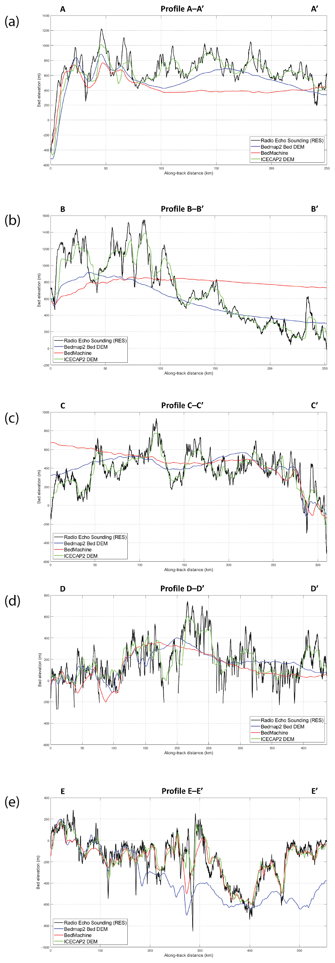
Figure 6 Bed elevations recorded in ICECAP2 RES transects (black), Bedmap2 (blue), BedMachine (red), and ICECAP2 DEM (green). (a) Profile A–A^′, (b) profile B–B^′, (c) profile C–C^′, (d) profile D–D^′, and (e) profile E–E^′. See Fig. 4b for transect locations.

Table 1 Data files and locations.

We also present five terrain profiles for all three DEMs (Fig. 6), which collectively cover most of the PEL sector (Fig. 1c). The purpose is to understand how much of the subglacial morphology is captured in each DEM, and to assess the relative accuracy of the DEMs in their characterization of subglacial topography. In general, and as one would expect, the ICECAP2 bed DEM shows reasonable agreement with the RES transects in all profiles. Consistencies between the ICECAP2 DEM and the bed elevation from RES data picks can be seen in profiles A and B with correlation coefficients of 0.83 (RE – 3 %) and 0.97 (RE – 1 %), respectively. These are higher relative to both the Bedmap2 and BedMachine DEMs, which are 0.74 (RE – 19 %) and 0.56 (RE – 36 %) for profile A and 0.89 (RE – 11 %) and 0.07 (RE – 26 %) for profile B, respectively. A significant improvement is also noted in the ICECAP2 DEM across the American Highland in profile C (Fig. 6), with a correlation coefficient of 0.91 (RE – 5 %) compared to 0.59 (RE – 9 %) for Bedmap2 and 0.33 (RE – 11 %) for BedMachine. A slightly lower correlation coefficient is quantified for the ICECAP2 DEM in profile D, at 0.85 (RE – 17 %), but it is still higher than in Bedmap2, at 0.57 (RE – 32 %), and BedMachine, at 0.54 (RE – 48 %). In profile E (near to Wilhelm II Land), the ICECAP2 DEM correlation coefficient is slightly higher, at 0.91 (RE – 0.5 %), than BedMachine, at 0.87 (RE – 0.37 %), and much higher than in Bedmap2, at 0.57 (RE – 40 %). While the gross subglacial morphology of PEL is captured well by the ICECAP2 DEM, much of the short wavelength roughness recorded in the RES data is smoothed out (Fig. 6). Forming a DEM that captures such detail requires further data acquisition, especially between existing RES profiles. As short wavelength bed roughness is critical to ice flow (e.g. Hubbard et al., 2000), such measurements in PEL, and indeed elsewhere in Antarctica, are now a scientific priority (Kennicutt et al., 2019).

6 Data availability

The ICECAP2 ice thickness and bed elevation models of the PEL sector are available in 500 m horizontal resolutions at https://doi.org/10.5281/zenodo.4023343 (Cui et al., 2020a). The airborne RES ice thickness measurements used to generate the products, recorded here in comma-separated values (CSVs) format, are accessible from https://doi.org/10.5281/zenodo.4023393 (Cui et al., 2020b). The 500 m ice sheet surface elevation DEM derived from the REMA (Howat et al., 2019) can be obtained from https://www.pgc.umn.edu/data/rema/ (last access: 12 September 2020). If the users wish to modify the bed DEM, our model can be easily integrated with the updated surface elevation models (Bamber et al., 2009; Helm et al., 2014). Auxiliary details for the MEaSUREs InSAR ice velocity map of Antarctica can be found at https://doi.org/10.5067/D7GK8F5J8M8R (Rignot et al., 2017b). The satellite images from the MODIS Mosaic of Antarctica (2008–2009) are obtainable from https://doi.org/10.7265/N5KP8037 (Haran et al., 2014, updated in 2019). A summary of the data used in this paper and their availability is provided in Table 1.

7 Summary

We have presented RES data from the first dedicated airborne geophysical survey of PEL. From the data (and using a combination of interpolation and modelling techniques), we have generated a bed DEM at a resolution of 500 m over an area of ∼900 000 km² – the ICECAP2 DEM. Considerable differences between this DEM and both Bedmap2 and BedMachine Antarctica are observed, particularly at the centre of the DEM where a broad subglacial basin has been identified and measured. The ICECAP2 DEM completes the first-order data coverage of subglacial Antarctica – a feat spanning around 70 years of international collaboration (Turchetti et al., 2008).