A combined Terra and Aqua MODIS land surface temperature and meteorological station data product for China from 2003 to 2017

Land surface temperature (LST) is a key variable for high temperature and drought monitoring and climate and ecological environment research. Due to the sparse distribution of ground observation stations, thermal infrared remote sensing technology has become an important means of quickly obtaining ground temperature over large areas. However, there are many missing and low-quality values in satellite-based LST data because clouds cover more than 60 % of the global surface every day. This article presents a unique LST dataset with a monthly temporal resolution for China from 2003 to 2017 that makes full use of the advantages of MODIS data and meteorological station data to overcome the defects of cloud influence via a reconstruction model. We specifically describe the reconstruction model, which uses a combination of MODIS daily data, monthly data and meteorological station data to reconstruct the LST in areas with cloud coverage and for grid cells with elevated LST error, and the data performance is then further improved by establishing a regression analysis model. The validation indicates that the new LST dataset is highly consistent with in situ observations. For the six natural subregions with different climatic conditions in China, verification using ground observation data shows that the root mean square error (RMSE) ranges from 1.24 to 1.58 ^∘C, the mean absolute error (MAE) varies from 1.23 to 1.37 ^∘C and the Pearson coefficient (R²) ranges from 0.93 to 0.99. The new dataset adequately captures the spatiotemporal variations in LST at annual, seasonal and monthly scales. From 2003 to 2017, the overall annual mean LST in China showed a weak increase. Moreover, the positive trend was remarkably unevenly distributed across China. The most significant warming occurred in the central and western areas of the Inner Mongolia Plateau in the Northwest Region, and the average annual temperature change is greater than 0.1 K (R>0.71, P<0.05), and a strong negative trend was observed in some parts of the Northeast Region and South China Region. Seasonally, there was significant warming in western China in winter, which was most pronounced in December. The reconstructed dataset exhibits significant improvements and can be used for the spatiotemporal evaluation of LST in high-temperature and drought-monitoring studies. The data are available through Zenodo at https://doi.org/10.5281/zenodo.3528024 (Zhao et al., 2019).

1 Introduction

Land surface temperature (LST), which is controlled by land–atmosphere interactions and energy fluxes, is an essential parameter for the physical processes of the surface energy balance and water cycle at regional and global scales (Li et al., 2013; Wan et al., 2014; Benali et al., 2012). LST datasets not only are required for high-temperature and drought research over various spatial scales but also are important elements for improving global hydrological and climate prediction models. In particular, the LST directly influences glaciers and snow on the Qinghai–Tibet Plateau (Tibetan Plateau), which is known as the “world water tower”. In turn, these changes directly affect the living conditions of nearly 40 % of the world's population (Xu et al., 2008). Therefore, LST research at regional and global scales is crucial for further improving and refining global hydroclimatic and climate prediction models. LST is measured by meteorological stations which have the advantages of high reliability and long time series. However, the meteorological station data collected as point data with very limited spatial coverage are often sparsely and/or irregularly distributed, especially in remote and rugged areas (Neteler, 2010; Hansen et al., 2010; Gao et al., 2018). To obtain spatially continuous LST data, various geostatistical interpolation approaches are commonly applied to achieve spatialization, such as kriging interpolation and spline function methods. However, the smoothed spatial pattern obtained after interpolation may suffer from low reliability because the ground station density is far from sufficient in most regions.

In contrast to ground-based observations with their limited availability and discrete spatial information, images captured by satellite thermal infrared instruments have become reliable alternative data sources with the advantages of detailed spatialized surfaces and near-real-time data access (Vancutsem et al., 2010). For instance, for the study of uniform continuous surface temperatures over large-scale areas, such as at regional and global scales, satellite remote sensing is the only efficient and feasible method (Xu et al., 2013). Satellite remote sensing obtains global LSTs based on a variety of mature retrieval algorithms that have been proposed since the 1970s for use with data from thermal infrared channels (McMillin, 1975). Due to its optimal temporal coverage and its global coverage, the Moderate Resolution Imaging Spectroradiometer (MODIS) sensor has become an excellent data source for satellite-derived LST data, and the MODIS LST values are widely used in regional and global climate change and environmental monitoring models (Tatem et al., 2004; Wan et al., 2014). However, satellite-derived LST data are frequently and strongly affected by data gaps and cloud cover, which affect the quality of the LST product. Cloud cover is frequent, and the locations of cloud cover are often uncertain. On average, at any one time, approximately 65 % of the global surface is obscured by clouds, leading directly to missing values over large, unevenly distributed areas in an image (Crosson et al., 2012; Mao et al., 2019). Although the integrity of the data has been greatly improved, the 8 d and monthly composite data still contain a number of low-quality pixels because these are derived from daily LST pixels. Invalid and low-quality surface temperature data make temperature products discontinuous in time and space, which leads to great restrictions on the use of temperature products. Thus, it is necessary to reconstruct these missing and low-quality LST pixels for satellite-derived LST applications.

Two categories of methods have commonly been applied to reconstruct missing pixels and pixels exhibiting low-quality data due to, e.g., cloud and/or aerosol influence, henceforth termed cloud low-quality pixels from satellite-derived data in previous studies. The first category includes methods that directly reconstruct missing and low-quality values using neighboring information with high similarity over temporal and spatial scales. Most temporal interpolation methods reconstruct missing and low-quality LST values based on the periodic behavior of data, such as harmonic analysis of time series (HANTS), Savitzky–Golay (S–G) filtering and the Fourier transform (Xu and Shen, 2013; Na et al., 2014; Scharlemann et al., 2008). Crosson (2012) used another temporal interpolation method to reconstruct the LST data from the Aqua platform (afternoon overpass) using LST data from the Terra platform (morning overpass). Regarding spatial interpolation methods, previous methods have focused on geostatistical interpolation, including kriging interpolation, spline interpolation and their variants. Some researchers have also carried out other attempts. For example, Yu et al. (2015) introduced a method using a transfer function with the most similar pixels to estimate invalid pixels. These methods, which estimate missing MODIS LST data using only adjacent high-quality MODIS LST data, take advantage of the similarity and interdependence of the available temporal or spatial attributes of neighboring pixels. To some extent, these methods have the advantage of simplicity and reliability. However, this category of methods is often not as reliable as expected especially in complex topographical regions and areas with many missing data in space and over time, because data coverage is too sparse for a reliable reconstruction. The second category of methods solves these data gap problems by establishing correlation models for cloud low-quality pixels and corresponding auxiliary data pixels. Neteler (2010) used a digital elevation model (DEM) as an auxiliary predictor to reconstruct MODIS LST data from 9 years of data on temperature gradients, which achieved reliable results in mountainous regions. Ke et al. (2013) built a regression model that included many auxiliary predictors – latitude, longitude, elevation and the normalized difference vegetation index (NDVI) – to estimate 8 d composite LST products. Fan et al. (2014) used multiple auxiliary maps, including land cover, NDVI and MODIS band 7, to reconstruct LST data in flat and relatively fragmented landscape regions. Other similar algorithms have drawn support by employing many factors that affect LST, including elevation, NDVI, solar radiation, land cover, distance from the ocean, slope and aspect. Considering the complexity of the terrain and the nonuniformity of the spatial distribution of large-scale LST patterns, a reconstruction model with auxiliary data that provides rich information for missing pixels can improve the accuracy of the interpolation result.

The above studies greatly improved the usability of MODIS LST data and further added value to long-term LST trend analyses. However, despite the use of various techniques to reconstruct the LST value, existing techniques focus on the retrieval of the LST value under the assumption of clear-sky conditions. However, clouds reduce nighttime surface cooling and daytime surface warming due to solar irradiance. These effects are not taken into account using this assumption, and therefore the derived LST values are likely biased towards clear-sky conditions. To address this issue, some scholars have also used microwave temperature brightness (TB) data, which are mostly derived from high-frequency channels (≥85 GHz), to obtain the LSTs under clouds (André et al., 2015; Prigent et al., 2016). Although microwave remote sensing is more capable of penetrating clouds than thermal remote sensing, the physical mechanisms of the current microwave LST retrieval models are not very mature (Mao et al., 2007, 2018). Moreover, due to the difference in the surface properties of the land, the depth of the radiation signal detected by the microwave will differ at different locations, and it will deviate from the retrieval results of thermal infrared remote sensing when used to estimate LST values. Thus, new reconstruction methods for LST data need to be proposed to compensate for this deficiency.

On this premise, China is used as an example due to its large coverage area, heterogeneous landscape and complex climatic conditions. This paper presents a new long-term spatially and temporally continuous MODIS LST dataset in a monthly temporal and 5600 m spatial resolution for China from 2003 to 2017 that filters out invalid pixels (missing-data influence by cloud and rainfall) and low-quality pixels (average LST error >1 K) and reconstructs them based on multisource data. We describe a data reconstruction process that is fully integrated with the benefits of the high reliability of surface observations, consistency and high accuracy of daily valid pixels, and spatial autocorrelation of similar pixels. The process compensates for the insufficiency of reconstructing pixels under clear-sky conditions instead of under clouds in previous studies. The validation using data from the China Meteorological Administration observations indicates the robustness of the LST data after interpolation. The dataset is ultimately used to capture the annual, seasonal and monthly spatiotemporal variations in the LST in six natural subregions in China. It is envisioned that this dataset will help capture changes in surface temperature and will be useful for studies on high temperatures, drought and food security.

2 Study area

In order to obtain a set of continuous spatial and temporal datasets of surface temperature in China and explore the temporal and spatial characteristics of China's LSTs, the study area is divided into six natural subregions based on China's three major geographical divisions: climatic conditions, landform types and tectonic movement characteristics. The eastern region is topographically characterized by plains and low mountains. This region has a variety of monsoon climate zones, which, from south to north, include tropical, subtropical and temperate monsoon climate zones. Therefore, we divide the eastern region into the following four regions, as shown in Fig. 1. (I) The Northeast Region, which mainly covers the area to the east of Daxing'anling. This region has a temperate monsoon climate with an average annual precipitation of 400–1000 mm, and rain and heat are prevalent in the same period. (II) The North China Region lies to the south of the Inner Mongolia Plateau, to the north of the Qinling Mountains and Huai River, and to the east of the Qinghai–Tibet Plateau. The region is dominated by a temperate monsoon climate and a temperate continental climate with four distinct seasons. This area is characterized by flat plains and plateau terrain. (III) The Central Southwest China Region extends from the eastern part of the Qinghai–Tibet Plateau to the western parts of the East China Sea and South China Sea, south to the Huai River–Qinling Mountains, and north to the area where the daily average temperature is greater than or equal to 10 ^∘C. The accumulated temperature in this region is 7500 ^∘C. This region is commonly dominated by a subtropical monsoon climate. (IV) The South China Region is located in the southernmost part of China and is characterized by a tropical and subtropical monsoon climate with hot and humid conditions. The area has abundant rainfall, and the average annual precipitation is approximately 1900 mm.

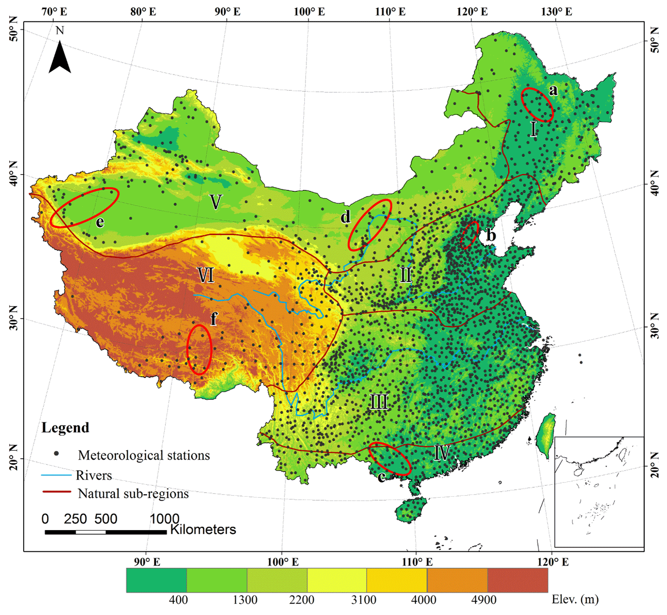
Figure 1 The study area is divided into six natural subregions (I, II, III, IV, V and VI), and the spatial distribution of the meteorological stations in the subregions is shown. The red ellipses mark key areas where the temperature has changed significantly, and meteorological stations from subset (2) located in these areas referring to Sect. 3.2 are used to validate the accuracy of the new LST dataset (a, b, c, d, e and f).

The western region is divided into two natural subregions. (V) The Northwest Region includes the northern Qilian Mountains–Altun Mountains–Kunlun Mountains, the Inner Mongolia Plateau and the western part of the Greater Khingan Range. This region is located in the continental interior and features complex terrain conditions, dominated by plateau basins and mountainous areas. This region has a tropical dry continental climate with rare rainfall. Consequently, this area features large areas of barren land, with a desertified land area of 2.183 million km², accounting for 81.6 % of China's desertified land area (Deng, 2018). Moreover, the Taklamakan Desert in this region is one of the 10 largest deserts in the world. (VI) The Qinghai–Tibet Plateau region is mainly located on the Qinghai–Tibet Plateau, which is the highest-elevation plateau in the world. This region is mainly described as having an alpine plateau climate, with relatively high temperatures and an extensive grassland meadow area.

3 Data and methods

3.1 MODIS data

MODIS is a key sensor of the Earth Observing System (EOS) program that provides a suite of various products with global coverage of the land, atmosphere and oceans. MODIS covers 36 spectral bands in the visible, near-infrared and thermal infrared ranges (from 0.4 to 14.4 µm), so it is extensively used to study global marine, atmospheric and terrestrial phenomena (Wan et al., 1997). The MODIS instruments are aboard two NASA satellites, Terra and Aqua, which were launched in December 1999 and May 2002, respectively. As both the Aqua and Terra satellites are polar-orbiting satellites flying at an altitude of approximately 705 km in sun-synchronous orbit, they provide data twice daily. The Terra satellite passes through the Equator at approximately 10:30 and 22:30 local solar time and is called the morning satellite. The Aqua satellite passes through the Equator at approximately 01:30 and 13:30 and is called the afternoon satellite (Vancutsem et al., 2010). Each satellite covers the global twice a day and transmits observation data to the ground in real time.

MODIS LST data are retrieved with two algorithms: the generalized split-window algorithm (Wan and Dozier, 1996; Wan et al., 2002) and the day/night algorithm (Wan and Li, 1997). We use MOD11C1–MYD11C1 and MOD11C3–MYD11C3 from the last generation of V006 products which utilizes the day/night algorithm. The day/night LST algorithm exhibits great advantages in retrieving LST: it not only optimizes atmospheric temperature and water vapor profile parameters for optimal retrieval but also does not require the complete reversal of surface variables and atmospheric profiles (Wan, 2007; Ma et al., 2000, 2002). A comprehensive sensitivity and error analysis was performed for the day/night algorithm, which showed that the accuracy was very high, with an error of 1–2 K in most cases (0.4–0.5 K standard deviation over various surface temperatures for midlatitude summer conditions; Wan and Li, 1997; Wang and Liang, 2009; Wang et al., 2007). The datasets include daytime and nighttime surface temperature data provided by NASA. In collection 6 data, the identified cloud low-quality LST pixels were removed from the MODIS Level 2 and Level 3 products, and the classification-based surface emissivity values were adjusted (Wan, 2014). Both datasets provide the global LSTs generated by the day/night algorithm with a spatial resolution of $\mathrm{0.05}{}^{\circ }\times \mathrm{0.05}$^∘ (approximately 5600 m at the Equator), which is provided in an equal-area integerized sinusoidal projected coordinate system. The monthly (MOD11C3–MYD11C3) data are deduced from daily global data (MOD11C1–MYD11C1).

3.2 Supplementary data

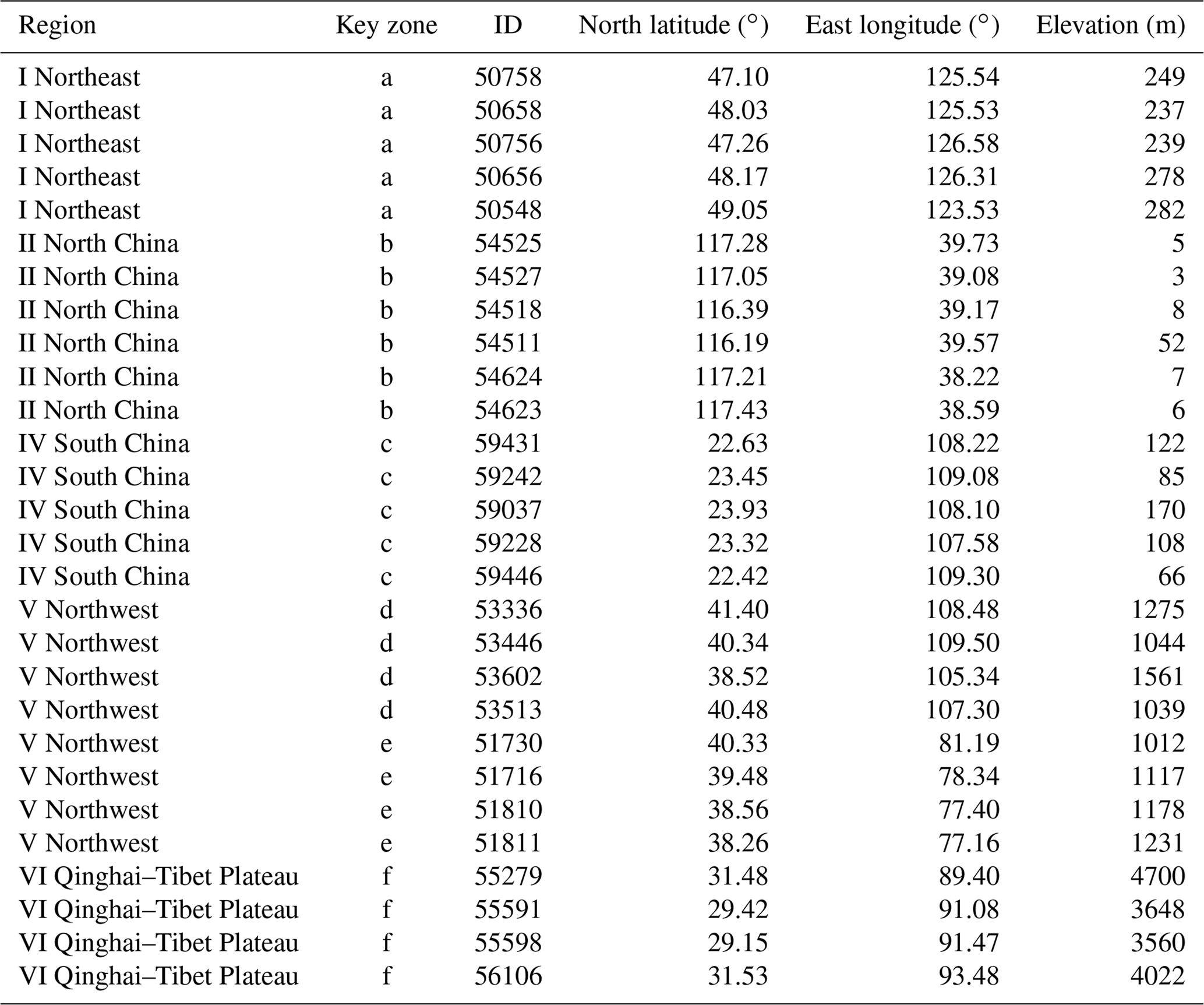
LST records at hourly intervals from 2399 meteorological ground stations in China from 2003 to 2017 were used in this study, and they were provided and subjected to strict quality control and evaluation by the China Meteorological Administration (CMA). Meteorological station data were randomly divided into two completely independent subsets by the jackknife method (Benali et al., 2012). In subset (1), the number of ground stations used for the reconstruction process was 1919, accounting for 80 % of the total number of ground stations. In subset (2), the number of sites used for verification was 480, accounting for 20 % of the total. Then, the data used for the reconstruction process for subset (1) were created by extracting meteorological station LST data at local overpass times. For the verification process, six key areas where positive or negative trends were the most significant (i.e., shown in the red ellipses a–f in Fig. 1 and Table 1) were selected as a representative area. The data of the ground weather station need to be checked manually because different stations are maintained by different personnel. Occasionally, some data may be abnormal, especially in remote sites due to instrument aging and lack of maintenance or insufficient power which causes data inaccuracy. All meteorological ground station data were tested for temporal and spatial consistency, which included identifying and rejecting extreme values and outliers. It is worth noting that the key areas marked by red ellipses contain site data from subset (1) and subset (2). Generally, there are more stations in the red ellipse than in the sites used for verification in Table 1, especially in eastern China where there are a large number of stations. The surface types of most sites are bare land, grassland and agricultural land. Elevation data with a 1 km resolution are obtained from the NASA Space Shuttle Radar Topography Mission (SRTM) V4.1 for reconstruction of cloud low-quality data (http://srtm.csi.cgiar.org/, last access: 24 August 2018).

Table 1 Basic information for some of the meteorological stations in key zones.

3.3 LST data restoration method

Although thermal infrared remote sensing technology can quickly obtain large-area surface temperature information, it can still be affected by factors such as clouds and rainfall. It is difficult to fill data gaps caused by clouds in LST data products based on satellite infrared imagery with data of the same quality as the clear-sky LST observations. Therefore, we create a reconstruction model that combines meteorological station data and daily and monthly MODIS LST data to reconstruct a high-precision monthly dataset that takes into account the actual LST under both clear-sky and cloudy conditions. The reconstruction model effectively preserves the highly accurate pixels in the original daily and monthly data, reconstructs only the low-quality daily data, and finally, replaces low-quality pixels with the composite average pixel value in the monthly data. To better describe the data processing, Fig. 2 shows a summary flowchart for the reconstruction of MODIS monthly LST data. The reconstruction model we propose is divided into two general steps: LST pixel filtering and LST data restoration. Low-quality pixel values were first identified and set to missing values for all input monthly LST images based on pixel quality filtering (see Sect. 3.3.1 for details). Both missing pixels and low-quality pixels are considered invalid pixels that need to be reconstructed. For each invalid pixel in the monthly images, we first determined the invalid pixels in daily LST images at the same location for all days of the respective month, and then we reconstructed these invalid daily pixels. The reconstruction process for the invalid daily pixels is divided into three steps (see Sect. 3.3.2 for details): (1) where possible we filled invalid grid cells with co-located in situ observations of the LST; (2) in case where in situ observations are lacking, we employed the geographically weighted regression (GWR) method to interpolate invalid pixels based on similar pixels from multiple sources; and (3) the remaining invalid grid cells we filled with LST values reconstructed based on regression of the elevation–temperature gradient. Finally, after we obtained four temperature values corresponding to the four products of MODIS LST every day, we averaged over daily data of the respective month and replaced the invalid data in the original monthly LST product with the new monthly LST value based on the reconstructed LST time series of that month.

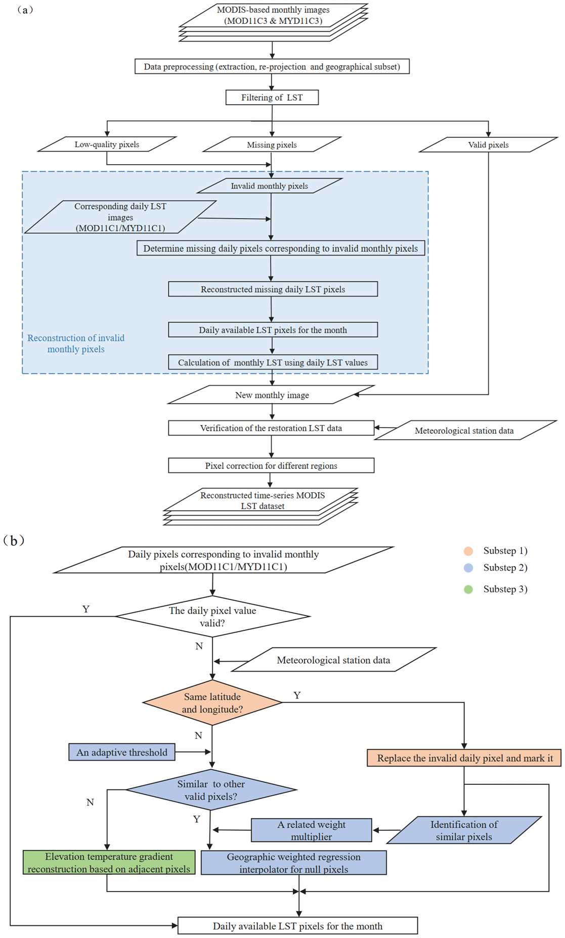
Figure 2 (a) The summary flowchart for reconstructing MODIS monthly LST data; (b) the detailed flowchart for reconstructing missing daily pixels in (a).

3.3.1 Filtering of MODIS LST

MODIS LST data are retrieved from thermal infrared bands in clear-sky conditions and contain many missing values and low-quality values caused by factors such as clouds and aerosols. Generally, the cold top surface of a thin or subpixel cloud is difficult to detect, and the LST retrieved under such conditions usually leads to an underestimation of LST (Neteler, 2010; Markus et al., 2010; Jin and Dickinson, 2010; Benali et al., 2012). Moreover, other factors can also contaminate the observation signal and cause the data to be unavailable, such as aerosols, observation geometry and instrumental problems (Wan, 2014). MODIS surface temperature products provide detailed product quality information, which is very convenient for us to judge and identify.

Cloud cover is extensive and inevitable in daily weather conditions. Statistical calculations were performed and showed that missing values for daily data reached approximately 50 % for Terra and Aqua satellites. Figure 3 shows an example representing the distribution of valid pixel values in the daytime for winter and summer. The coverage of pixels with missing data in the study area at 10:30 GMT+8 during the daytime on 1 January 2017 and 1 July 2017 for the Terra platform reached 44.9 % and 51.7 %, respectively. The spatial gaps in the daily data are characterized by an arbitrary distribution and generally large aggregations. In fact, the emergence of a large number of missing values every day makes it difficult to reconstruct high-precision LST under clouds using current techniques due to such a paucity of information, especially for areas with complex climates.

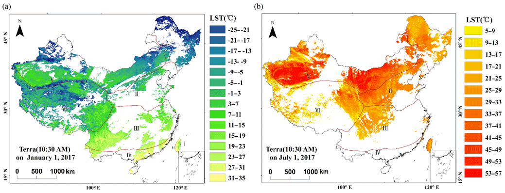
Figure 3 Spatial distribution of valid data for daily MODIS LST data from Terra during the daytime on (a) 1 January 2017 and (b) 1 July 2017. Areas of missing data are blank, and no filtering is performed (see text for details).

However, the random occurrence of cloud-covered areas has a much smaller impact on monthly composite products, which makes these products a reliable source for building a high-precision monthly LST dataset. Compared with daily and 8 d composite data, spatiotemporal integrity and consistency have been greatly improved in monthly composite LST data. However, for many regions, the lack of data or quality degradation caused by clouds is still common even in monthly composite data (Fig. 4). A reliable method for removing low-quality pixels is implemented using the data quality control information for MODIS LST data. The data quality control information is statistically calculated and stored in the corresponding quality assurance (QA) layer and is represented by an 8 bit unsigned integer and can be found in the original MODIS LST HDF files. Therefore, we use the quality control labels for daily and monthly files as mask layers to identify low-quality pixels to ensure the quality of the LST data. For monthly LST data, grid cells with QA layer labels of “theaverageLSTerror<=1 K”, “LST produced, good quality” and “theaverageemissivityerror<=0.01” are considered to be high-quality data, and the remaining pixels are low-quality pixels and are set to missing values. Since there are many pixels with missing value in the daily LST data due to clouds (as shown in Fig. 3), in order to ensure a sufficiently large number of pixels with daily LST values required for the reconstruction, only pixels with an LST error >3 K are rejected and set to missing values in the daily LST data. Our aim is to reconstruct the LST for all these grid cells with invalid data. A summary flowchart of the process used to construct the LST data model is schematically illustrated in Fig. 2.

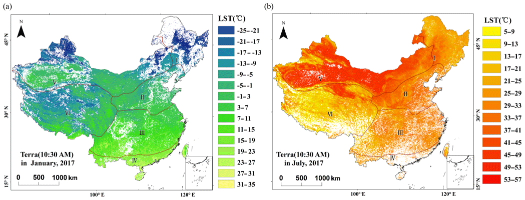
Figure 4 Spatial distribution of valid data after pixel filtering (see text for details) for monthly MODIS LST data from Terra during the daytime in (a) January and (b) July. Areas of invalid data are blank.

The spatial distribution pattern of invalid monthly Terra LST data after filtering by the QA layer is shown in Fig. 4. The low-quality pixel coverage rates for January and July 2017 were 23.45 % and 19.68 %, respectively. There are more missing values in winter than in summer in the northeastern region, which may be affected by the confusion resulting from large areas of snow cover and clouds in the winter. However, the missing values are mainly concentrated in southern China in summer, which is closely related to the increased cloud cover in the hot summers in South China.

3.3.2 LST data restoration

In the reconstruction model, we first filter each monthly image, and the locations of the cloud low-quality pixels (i.e., the missing and low-quality monthly pixels) are determined. Then, for each month, we filter all daily images of the respective month by determining all missing and low-quality grid cells. The valid pixels ${\overline{P}}_i$ in the daily data are retained, the low-quality daily data are reconstructed, and the low-quality pixels in the monthly data are replaced with the average LST derived from the gap-filled daily LST time series of the corresponding month (Fig. 2). Missing daily pixels are defined as the target pixels T_t; the image containing the target pixels T_t is the target image. The reconstruction process for the target pixels T_t is as follows.

When there are clouds in the sky, the surface temperature of different surface types is not consistent with the temperature of neighboring pixels during the day and night. Factors that affect reconstruction accuracy mainly include the NDVI, elevation, latitude and longitude. Grid cells with invalid LST values were co-located with meteorological stations based on the latitude and longitude information. Invalid pixels were filled using the values from valid in situ LST data at the same location at the same time, and these filled pixels were marked. Then, for the invalid pixels without ground meteorological station data, we used a combination of two strategies to reconstruct the missing LST data to improve the accuracy of the result. The first strategy identified the most similar pixels by using adaptive thresholds and reconstructed them by using a GWR method.

GWR is a common and reliable method for estimating missing pixels, which quantifies the contribution of each similar pixel to contaminated pixels. This method assumes that similar pixels that are spatially adjacent to the target pixel are close in the spectrum and should be given more weight. Due to the high temporal variability in thermal radiation emitted from the land surface and atmospheric state parameters, satellite sensors that measure the thermal radiation energy from different phase images at the same locations often produce different values even when the same thermal infrared sensor is used. Some of the most common regular changes in surface features, such as the vegetation spectrum changes due to plant growth, can be predicted using auxiliary information of surface meteorological observation stations.

Because the factors that influence surface temperature (vegetation cover, sun zenith angle, microrelief, etc.) vary greatly among different regions, the differences in adjacent pixels in different areas may also vary greatly. Thus, there will be large deviations in the similar-pixel decision criteria if a fixed similarity threshold is used. Here, we use an adaptive threshold φ^τ to determine similar pixels for each invalid pixel (Eq. 3). The adaptive threshold φ^τ calculated from the standard deviation indicates the local area smoothness. The local area is a certain size area centered on similar pixels, which is located in the three reference images. The closer the pixel is, the more similar the environment is, so the smoother the local area will be. For example, the jth valid pixel in the target image is determined to be a similar pixel to the target pixel i only when the relationship described in Eq. (2) is satisfied in the reference image τ. Simultaneously, similar pixels were determined based on all valid pixels in the image rather than on a sliding window because missing values are often arbitrarily clustered in a large area rather than scattered.

$$\begin{array}{}\text{(1)}& {\displaystyle }\mathrm{|}{P}_{\mathrm{s}}^{\mathit{\tau }}-P_{\mathrm{t}}^{\mathit{\tau }}\mathrm{|}\le {\mathit{\phi }}^{\mathit{\tau }},\text{(2)}& {\displaystyle }{\mathit{\phi }}^{\mathit{\tau }}=\sqrt{{\sum }_{i=\mathrm{1}}^n(P_{\mathrm{s}}^{\mathit{\tau }}-\mathit{\epsilon }{)}^{\mathrm{2}}},\end{array}$$

where $P_{\mathrm{s}}^{\mathit{\tau }}$ and ${\mathrm{P}}_{\mathrm{t}}^{\mathit{\tau }}$ are the values of pixels corresponding to the position of the similar pixel and the target pixel in the reference image, respectively. φ^τ is the threshold used to determine similar pixels. ε is the mean value of all pixels in the local area. τ is the reference image (value=1, 2, 3). Here, we set the range of the local area to 5 pixels by 5 pixels centered on the target pixel (Zeng et al., 2013). In this paper, the number of similar pixels to the target pixel in the target image should be greater than 4 to apply the GWR method to reduce the error due to an insufficient number of similar pixels.

After determining similar pixels, the invalid LST values (at the target pixels) are reconstructed through GWR. In theory, LST data from meteorological stations are the most reliable record, even in the case of thick cloud coverage. If there is ground observation site data, similar pixels are obtained directly from ground stations which are the most representative and can better reflect the LST under clouds than under clear-sky conditions. In the process of reconstructing missing pixels, the regression weight coefficient of a similar pixel is determined by its Euclidean distance from the target pixel. In addition, we assign a related weight multiplier to the marked ground station data based on the GWR. After selecting some of the marked pixels as experiments, it was found that the target pixels could be more accurately estimated when the relative multiweight values of the ground stations were set to 3 in this paper. Therefore, the weighting coefficients of similar pixels are determined by Eqs. (5) and (6).

$$\begin{array}{}\text{(3)}& {\displaystyle }D=\sqrt{{\left(x-x_{\mathrm{t}}\right)}^{\mathrm{2}}+{\left(y-y_{\mathrm{t}}\right)}^{\mathrm{2}}},\text{(4)}& {\displaystyle }{W}_i={\displaystyle \frac{\frac{M_{\mathrm{c}}}{D_i}}{{\sum }_{i=\mathrm{1}}^m\frac{M_{\mathrm{c}}}{D_i}+{\sum }_{j=\mathrm{1}}^n\frac{M_{\mathrm{g}}}{D_j}}},\text{(5)}& {\displaystyle }{W}_j={\displaystyle \frac{\frac{M_{\mathrm{g}}}{D_j}}{{\sum }_{i=\mathrm{1}}^m\frac{M_{\mathrm{c}}}{D_i}+{\sum }_{j=\mathrm{1}}^n\frac{M_{\mathrm{g}}}{D_j}}},\end{array}$$

where D represents the Euclidean distance from the similar pixel (i, j) to the target pixel t and x, y, x_t and y_t describe the locations of the similar pixel and target pixel. i and j represent similar pixels used to estimate the low-quality LSTs, i is a valid pixel, and j is a pixel assigned by the ground station. W_i and W_j describe the weight that similar pixels i and j contribute to the target pixels, respectively. m is the number of similar pixels that are not low-quality as assigned by clouds, and n is the number of similar pixels that are assigned by ground stations. M_c and M_g represent the weight coefficients of clear-sky pixels and ground station assignment pixels, respectively. In this paper, M_c and M_g are set at 1 and 3, respectively. Therefore, the GWR method can be represented as follows.

$$\begin{array}{}\text{(6)}& T_{\mathrm{t}}={\sum }_{i=\mathrm{1}}^m{W}_i\cdot T_i+{\sum }_{j=m+\mathrm{1}}^n{W}_j\cdot T_j,\end{array}$$

where T_t is the reconstructed LST value of a target pixel, T_i and T_j represent LST values for the similar pixel i and j, and the sum of W_i and W_j values is 1.

The elevation–temperature gradient regression method was used to reconstruct the remaining low-quality pixels that did not have enough similar pixels. In general, the elevation has a particularly significant effect on the spatial variation in the LST at the regional scale. Elevation is recognized as the most important factor that characterizes the overall spatial trend in LST (Sun et al., 2016; NourEldeen et al., 2020). DEM data and LST data are used to construct linear regression relationships for invalid pixels based on the clear-sky pixels in the neighborhood of a certain window size; these data are then used to predict the missing-value pixels by linear interpolation (Yan et al., 2020). After several simulations of the experimental pixel window size, the noise was found to be minimized when a sliding window of 19 pixels by 19 pixels was used, and this window size was considered to have the best complement value.

$$\begin{array}{}\text{(7)}& T_i=\mathit{\alpha }\times h_i+\mathit{\beta },\end{array}$$

where T_i is the surface temperature data after interpolation (unit – ^∘C); h_i is the elevation value of pixel i (unit – m); α is the influence coefficient of the elevation on the surface temperature, which is the regression coefficient; and β is the estimated intercept. Finally, we accurately crop the image to a China-wide image to ensure that the sliding pixel window reaches the edge of the study area.

3.4 Analysis of the LST time series trend

In this study, the slope of a linear regression describes the rate of LST cooling or warming and is calculated by Eq. (8). The slope value and correlation coefficient (R), calculated with Eq. (9), were selected to quantify the temporal and spatial patterns in the LST variations.

$$\begin{array}{}\text{(8)}& \mathrm{Slope}={\displaystyle \frac{{\sum }_{i=\mathrm{1}}^n\left(i{T}_i\right)-\frac{\mathrm{1}}{n}{\sum }_{i=\mathrm{1}}^{n}i{\sum }_{i=\mathrm{1}}^n{T}_i}{{\sum }_{i=\mathrm{1}}^n{i}^{\mathrm{2}}-\frac{\mathrm{1}}{n}({\sum }_{i=\mathrm{1}}^{n}i{)}^{\mathrm{2}}}},\end{array}$$

$$\begin{array}{}\text{(9)}& R={\displaystyle \frac{n{\sum }_{i=\mathrm{1}}^n\left(i{T}_i\right)-{\sum }_{i=\mathrm{1}}^{n}i{\sum }_{i=\mathrm{1}}^n{T}_i}{\sqrt{n{\sum }_{i=\mathrm{1}}^n{i}^{\mathrm{2}}-({\sum }_{i=\mathrm{1}}^{n}i{)}^{\mathrm{2}}}\sqrt{n{\sum }_{i=\mathrm{1}}^n{T}_i^{\mathrm{2}}-({\sum }_{i=\mathrm{1}}^n{T}_i{)}^{\mathrm{2}}}}},\end{array}$$

where i is the number of years, T_i is the average LST of year i, and n is the length of the LST time series; here, n is 15. A positive slope indicates an increase in LST (warming); a negative slope indicates a decrease in LST (cooling). The R values range from −1 to 1. An R value greater than 0 means that the LST is positively correlated with the time series, and an R value less than 0 means that the LST is negatively correlated with the time series. Meanwhile, the larger the absolute value of R, the stronger the correlation with the time series changes.

4 Results

MODIS exhibits good performance in retrieving LST data, which has been verified by various studies (Wan et al., 2004; Wan, 2008, 2014; Wan and Li, 2011). Furthermore, to better evaluate the accuracy of the new dataset, we performed verification for the original data, low-quality data and reconstructed data in different regions of China. In this study, three statistical accuracy measures are used to evaluate the accuracy of the calibration: the square root of the Pearson coefficient (R²), root mean square error (RMSE) and mean absolute error (MAE). In addition, we use the reconstructed data products to perform application analysis to indirectly prove the accuracy of the data and their practical application value.

4.1 Evaluation of the original product

We conducted a comparative analysis based on the distribution of six natural subregions (I, II, III, IV, V and VI) in Fig. 1. Figure 5 shows scatter diagrams relating ground station data and original MODIS LST monthly data (MOD11C3–MYD11C3) without QA filtering. It can be seen from Fig. 5 that for each region, the deviation of some points causes the distribution of points to be more discrete. Validation using ground observation data shows that the root mean square error (RMSE) ranges from 1.39 to 1.61 ^∘C, the mean absolute error (MAE) varies from 1.25 to 1.52 ^∘C and the Pearson coefficient (R²) ranges from 0.91 to 0.98.

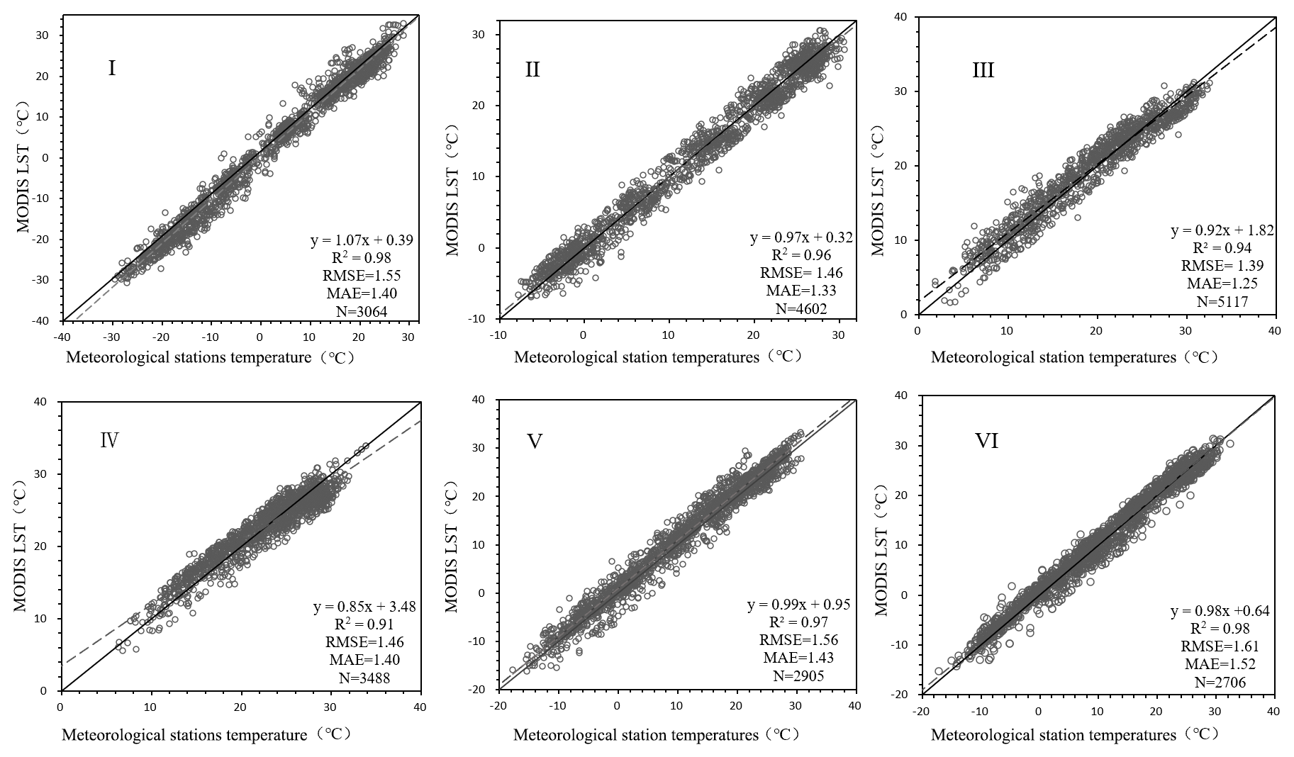
Figure 5 Scatter diagrams of original MODIS LST monthly data (MOD11C3–MYD11C3) against ground station data (N is the number of datasets); the statistical accuracy measures (R², RMSE and MAE) are also indicated.

4.2 Evaluation of the new product

In order to separately evaluate the improved accuracy of the low-quality area pixels of MODIS LST monthly products, we made a comparative analysis by partition. Figure 6 shows scatterplots of the low-quality MODIS LST data and reconstructed results versus their corresponding ground station data which show the accuracy comparison of low-quality pixels before and after reconstruction more clearly. The detailed comparative analysis of the partitions can be seen from Fig. 6, showing that the overall result between the reconstructed MODIS LST data and the ground station data presents a better linear relationship, with more clustered distribution on both sides of the 1:1 line. The accuracy of the reconstructed data in different low-quality regions is that the root mean square error (RMSE) ranges from 1.52 to 1.65 ^∘C, the mean absolute error (MAE) varies from 1.4 to 1.51 ^∘C and the Pearson coefficient (R²) ranges from 0.94 to 0.98, which is improved by more than 0.5 ^∘C compared with the original value.

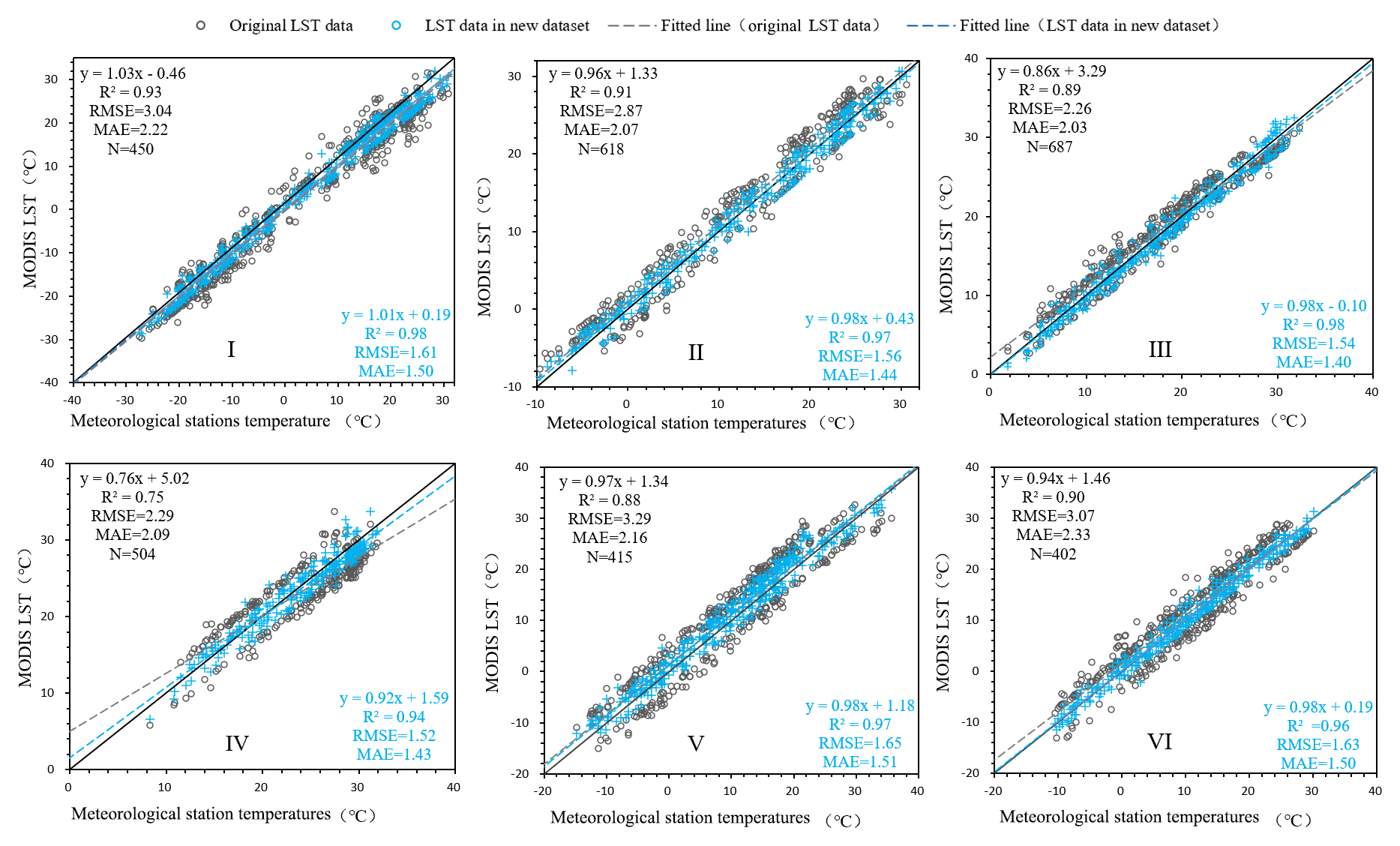
Figure 6 The scatter diagrams of the low-quality MODIS LST data and reconstructed results versus their corresponding ground station data in six natural subregions (I, II, III, IV, V and VI). The gray points indicate low-quality LST pixel values in the original MODIS LST data. The blue points represent the values in the new LST dataset, and the statistical accuracy measures (R², RMSE and MAE) are also indicated.

Figure 7 is an overall evaluation of the new dataset, which shows the statistical results of the difference between the two types of data in the six natural subregions (shown in blue in the scatterplot). According to the scatterplots of the ground station data and the reconstructed monthly MODIS LST data shown in blue in Fig. 7, we employed a correction model that uses the results of linear regression analysis between the two datasets to further improve the accuracy. The goal of the calibration model is to reduce or eliminate the combined error introduced by various variables. Therefore, the six subregions with different climatic conditions are corrected separately to obtain better calibration results for the study area. Additionally, to eliminate contrasts at the boundaries among the six regions, smooth constraints are imposed on some edge pixels with significant differences to guarantee consistency among the regions. The comparisons of the corrected LST data with the ground station data are indicated by the gray points in Fig. 7. In this study, the main reason for adopting the regression analysis model is the reality that a linear model can further improve the robust reconstruction results that have been obtained through a large amount of work. The results show that the model reconstruction results are highly consistent with the ground station data; thus, the problem of underestimation of MODIS LST data in some areas has been reduced.

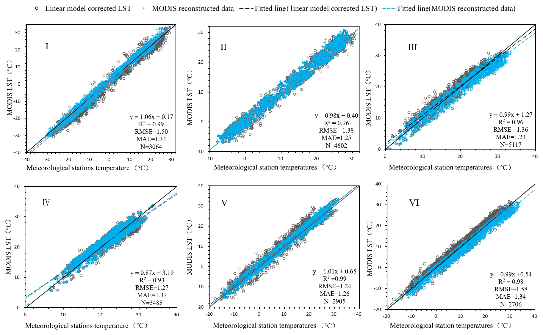
Figure 7 The scatter diagrams in six natural subregions (I, II, III, IV, V and VI) between the ground station data and the monthly MODIS LST data. The blue points represent the verification results of the reconstructed MODIS LST, and the statistical accuracy measures (R², RMSE and MAE) are also indicated. The results of the corrected linear model are indicated in gray.

All subregions showed good agreements between MODIS LST and meteorological station data. The R² values varied from 0.93 to 0.99, with an average of 0.97. The MAE varied from 1.23 to 1.37 ^∘C, with an average of 1.30 ^∘C. The RMSE ranged from 1.24 to 1.58 ^∘C, with an average of 1.39 ^∘C. A relatively large RMSE between the reconstructed LST and ground-based LST appeared in some sites in the Qinghai–Tibet Plateau region, indicating that the temperature exhibited great spatial heterogeneity over the complex terrain. As shown in Fig. 1, there are relatively few meteorological stations in western China. Under the same conditions, the accuracy in western China is lower than that in areas with dense weather stations when using surface meteorological stations to reconstruct LST values under cloudy conditions. The east and south of China are connected to the Pacific Ocean, so the amount of water vapor (clouds) in the sky is higher than in the west (like in Figs. 3 and 4). In this case, the number of days in which LST values can be obtained from the remote sensing images in a month is much smaller in eastern China than in western China. In this study, the accuracy evaluation is based on the monthly scale. The accuracy is mainly determined by the number of days of effective pixels on the monthly and annual scales, and our analysis indicates that the more days of available pixels corresponding to the pixels on the monthly scale, the higher the accuracy. These results indicate that the reconstructed MODIS LST dataset is robust and accurate due to its high consistency with the in situ data. Therefore, we believe that the accuracy of LST data can be improved by this method.

To further understand the credibility of the data and clarify the limitations of the use of this method, we further assess the performance in terms of the seasonal bias and compare it with the original seasonal LST data. Verification ground stations in representative areas are selected to help illustrate the distribution of the error in the reconstructed data. Six key zones are identified, corresponding to the areas a, b, c, d, e and f shown by the red ellipses in Fig. 1, and an overview of the ground stations can be found in Table 1. The six key zones are selected, including the three most significant regions for warming (b, d and f), the two most significant regions for cooling (a and c) and the zone located in Xinjiang Province (see Fig. 6a for details). Zone (a) located in the Northeast Region and zone (b) located in the North China Region experienced the strongest negative trend and significant warming, respectively. In particular, special attention has been given to the area around the Taklamakan Desert (e) in Xinjiang, which has complex terrain and extensive heterogeneity.

Seasonal-scale verification was performed using the RMSEs between the MODIS data (including the original LST and reconstructed LST data) and ground-based LSTs for comparison in the six key zones, as shown in Table 2. The original MODIS monthly LST data were used directly without filtering quality flags. For the original MODIS LST images, we averaged the LST data of the month corresponding to the season and obtained the seasonal LST images. The pixels with missing LST values in original MODIS LST images for the corresponding months of the season were not used in the verification process. Therefore, if there is no missing value for the LST pixel corresponding to the site, each station can have a maximum of 15 values in each season. Compared with that of the original LST, the average RMSE of the reconstructed LST data decreased by 18 % from 1.79 to 1.46 ^∘C. Both datasets exhibited the largest RMSE in summer and the smallest in autumn, indicating that the original and reconstructed LST data have highly consistent seasonal patterns. For the reconstructed LST data, we further found that the RMSE values at some sites in the summer were significantly higher than those at other sites. The regions that exhibited high RMSE values were mainly distributed in western regions (Xinjiang, Inner Mongolia and the Qinghai–Tibet Plateau), while the values in the other three regions were relatively low. The main reason for this difference may be that there are relatively few ground observation sites and complex terrain in the western region. The average RMSE in autumn was the lowest at 1.07 ^∘C. The winter RMSE ranged from 0.04 to 3.81 ^∘C, with an average of 1.45 ^∘C. The distribution of the RMSE varied greatly between the eastern and western regions at the seasonal scale. The maximum RMSE values for all stations in the eastern typical zones (i.e., key zone a in the Northeast Region I and key zone b in the North China Region II) occurred in the cold winter, while the highest values for most sites in the western region occurred during the hot summer months (i.e., the remaining four zones). At the same time, the comparison results show that the mean RMSE was significantly higher in the western region than in the eastern region (mean 1.04 ^∘C in eastern regions I and II and 1.69 ^∘C in western regions IV, V and VI). A large RMSE between the reconstructed LST data and the ground-based LST data appeared in some locations in Inner Mongolia (i.e., key zone e) in the Northwest Region, further indicating that we need to arrange more ground meteorological observation stations in these areas if we want to further improve the accuracy.

Table 2 RMSEs of seasonal LST between monthly LST data (including the original LST data and reconstructed LST data) and ground-based LST data (Orig. indicates original LST values at the ground stations; Recon. indicates the reconstructed LST values at the ground stations).

We also note that the selected ground stations shown in Table 2 located in six key zones are examples of where the local LST warming or cooling rate changed by more than the average rate, and these areas actually include areas with greater terrain complexity. Moreover, the examples indicate that the reconstruction model proposed here is effective even in the areas of complex topography.

The verification results show that the dataset has reasonable consistency with the in situ measurements, indicating that the interference of cloud coverage is well eliminated. The dataset obtained after reconstruction is a large-scale, long-term, unique surface temperature dataset because it eliminates low-quality pixels caused by factors such as cloud disturbance and achieves complete coverage of the entire study region. The accuracy and spatiotemporal continuity of this dataset are much better than those of the original MODIS monthly data. Moreover, in this dataset, the ground surface temperatures under cloud coverage are retrieved instead of reconstructing the LST under clear-sky conditions, which is better than the methods used in many previous studies.

4.3 The application of the product for trend analysis

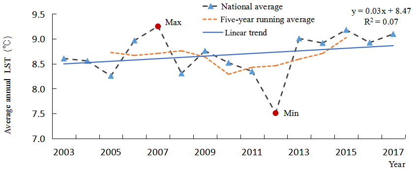
We carried out a lot of analysis in 2017 and found that the mean surface temperature of MODIS surface temperature in four time periods is close to the annual mean surface temperature because the observation time of the MODIS sensor is symmetrical, so it is feasible to use the monthly mean instead of the annual mean. Detailed derivation and comparative analysis of how to calculate the average temperature can be referred to in Mao et al. (2017). After LST data restoration data reconstruction, four overpass times of images are obtained each month, and seasonal and annual average spatial data are also obtained by adding averages. Further, we obtain the corresponding statistical values through equal-area projection calculations (Mao et al., 2017). Figure 8 shows the annual average LST change in China over the period from 2003 to 2017. The LST fluctuations in China exhibited a general weak positive trend. The sliding average of the 5-year unit also showed a weakly fluctuating positive trend. The lowest LST in China appeared in 2012 at 7.51 ^∘C. The temperature reached its highest value in 2007 (9.26 ^∘C), but after 2012, the LST remained high. This result coincides with the global warming stagnation period that was noticed from 1998 to 2012, and the LST increased significantly after 2012. After analyzing the LST on the seasonal and monthly scales, we found that the cooling in 2012 mainly occurred in the winter, as it was concentrated from January to February, and the cooling in the southern region was more significant than that in the other regions. In 2012, due to the abnormally strong East Asian winter monsoon, there was abnormal rainfall in the south in winter. Increased precipitation leads to increased evaporation, which leads to a decrease in temperature. We also observed a sudden decrease in LST in 2008 and a sudden increase in 2013. In 2008, severe persistent low-temperature snowstorm events in southern China in winter caused a decline in LST. The warming in 2013 was mainly affected by the abnormally high temperatures in the middle and lower reaches of the Yangtze River in summer. These indirectly verify the correctness of the reconstructed data through meteorological events, indicating that the reconstructed data can be used to analyze the long-term spatiotemporal changes in surface temperature.

Figure 8 Annual mean LST changes in China from 2003 to 2017.

For a more detailed understanding of the spatial patterns and regional differences in the LST changes in different areas, the rate of annual average LST change per pixel from 2003 to 2017 was calculated, and the slope (Fig. 9a), correlation coefficient (R; Fig. 9b), frequency distribution of the slope (Fig. 9c) and significance of the trend (P; Fig. A1) are shown. From 2003 to 2017, the annual average LST in China showed a weakly positive trend. The LST exhibited a strong positive trend in many regions in the north but negative trends in the south, and the positive trend in the west was greater than that in the east. Different regions showed significant regional variations. Most of China, accounting for 63.7 % of the study area, experienced a positive trend (slope>0; corresponding to the pale yellow, yellow, light orange, orange and red parts in Fig. 9c). Additionally, 20.8 % of the pixels experienced significant warming (slope>0.05, R>0.6, P<0.05). The areas with significant warming were mainly concentrated in the Inner Mongolia Plateau and areas to the south in the northwestern region. In contrast, 36.25 % of the areas showed a negative trend (slope<0, depicted in green and four shades of blue in Fig. 9c). The area with a significant cooling pattern (slope<−0.075, R<−0.6, P<0.05) covered 6.53 % of the study area, and these areas were mainly concentrated in the northeast. More analysis including monthly and seasonal changes can be found in the appendices.

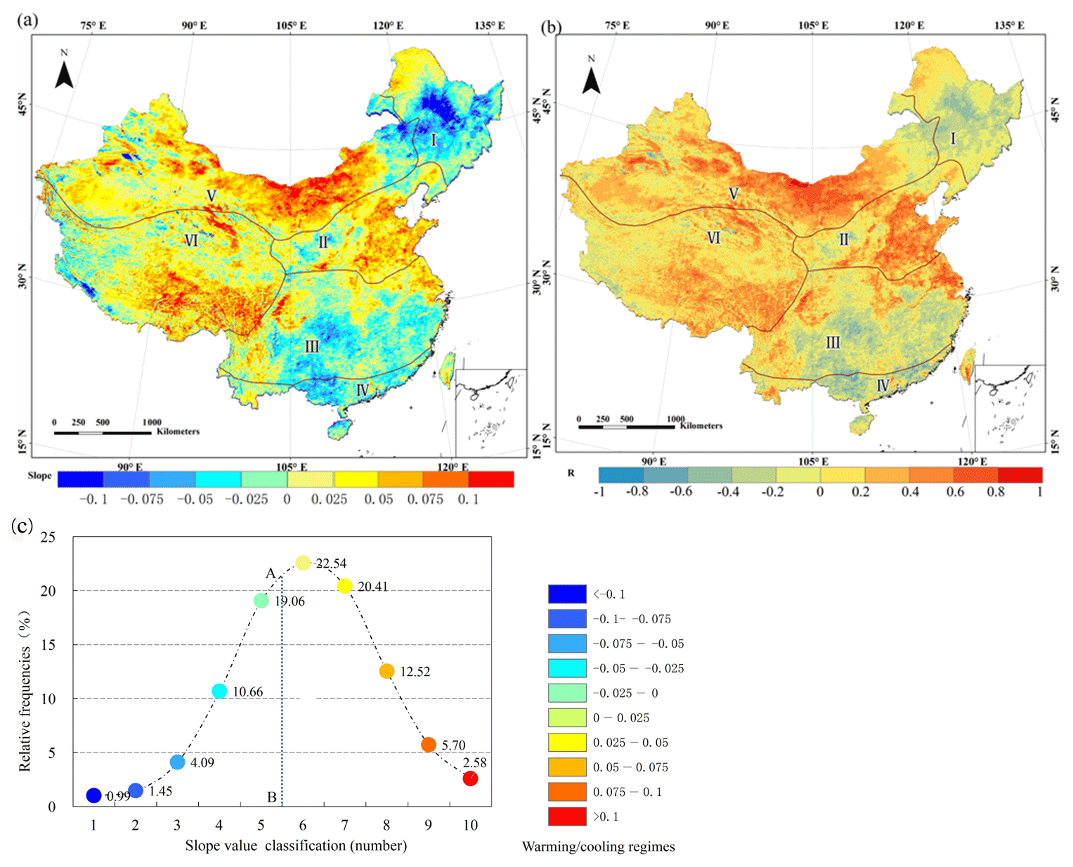
Figure 9 Spatial dynamics of interannual change trends in LST from the slope (a) computed by Eq. (8), the correlation coefficient (b) computed by Eq. (9) and frequency distribution of the slope (c) during 2003–2017. In panel (c), the different temperature trends (slope) are divided into 10 subinterval ranges corresponding to the ranges in panel (a). The area to the left of the line AB represents the proportion of the area that experienced cooling, and the area to the right represents the proportion that experienced warming.

5 Data availability

The dataset is needed for many geoscience studies, especially for studying regional climate change and thermal environment changes, agricultural drought, crop yield estimation, ecosystems, etc. The LST dataset in China is distributed under a Creative Commons Attribution 4.0 License. The dataset is named Land Surface Temperature in China (LSTC) and consists of two files. One is 00_Metadata for LSTC.docx, and the other is 01_LSTC.zip which contains data of LSTC. Each folder has 12 images (one scene per month). Each phase consists of two files, namely *.TIF (LSTC image) and *.TFW (TIFF image coordinate information). More information and data are freely available from the Zenodo repository https://doi.org/10.5281/zenodo.3528024 (Zhao et al., 2019).

6 Discussion and conclusions

In 2013, the Intergovernmental Panel on Climate Change (IPCC) noted that climate warming is clear (IPCC et al., 2013). However, some areas of the Northeast Region (I) have shown a significant warming hiatus over the past 15 years, and these areas made the greatest contribution to China's negative trend. We observed widespread and relatively strong cooling regimes in most areas (i.e., the slope value ranged from −0.06 to less than −0.12; see Fig. 9a, b for details), especially in the north of the Northeast Plain (slope<−0.1, R<−0.8, P<0.05; see Fig. 9a, b and Fig. A1). In the North China Region (II), the North China Plain and the Yangtze River Delta in the south both exhibit obvious positive trends, and both are densely populated areas. In addition, the Central Southwest China Region (III) and the South China Region (IV) also showed negative trends, but the negative trend was stronger in the South China Region (for most of the area, slope<0.75, R<−0.8, P<0.05) than in the Central Southwest China Region. In the Northwest Region (V), some areas in the Tian Shan and the Inner Mongolia Plateau experienced significant positive trends (slope>0.10, R>0.8, P<0.01), and this area exhibited the strongest positive trend in China over the past 15 years. In the Qinghai–Tibet Plateau region (VI), the ecological environment is complex, and the unique plateau terrain and thermal properties of the surrounding areas play an important role in regulating the surrounding atmospheric circulation system. Because the Qinghai–Tibet Plateau is extremely sensitive to climate change, it is considered to be a key area of global climate change. Therefore, we have also paid close attention to the temperature changes on the Tibetan Plateau. As shown in Fig. 9a and b, an obvious positive trend was captured in the southern part of the Qinghai–Tibet region (slope>0.08), which should be emphasized. Additionally, the positive trend in the Qaidam Basin in the northeast is significantly higher (slope>0.1) than that in the surrounding area.

Based on the Terra and Aqua MODIS land surface temperature dataset and meteorological station data, a new LST dataset over China was established for the period from 2003 to 2017. This dataset effectively removed approximately 20 % of the missing pixels or low-quality LST pixels from the original MODIS monthly image. A detailed comparison and analysis with the in situ measurements shows that the reconstruction results have high precision, the average RMSE is 1.39 ^∘C, the MAE is 1.30 ^∘C and the R² is 0.97. The data are freely available at https://doi.org/10.5281/zenodo.3528024 (Zhao et al., 2019). We believe that this dataset will be of great use in research related to temperature, such as high temperature and drought studies, because it effectively overcomes the limitations of reconstructing the real LST under cloudy conditions in the past and achieves good spatiotemporal coverage.

The high-precision monthly LST dataset constructed for China provides a detailed perspective of the patterns of the spatial and temporal changes in LST. The LST dataset was used to analyze the regional characteristics and capture the variations in LST at the annual, seasonal and monthly scales. Our results showed that the LST showed a slight upward trend with a slope of 0.026 (approximately 63.7 % and 20.80 % of the pixels underwent warming and significant warming, respectively). There were great regional differences in the climate positive trend. The Northwest Region, the Qinghai–Tibet Plateau region and the North China Plain experienced significant positive trends (i.e., the slope ranged from 0.025 to greater than 0.1). The impacts of human activities on warming are prominent, such as the increase in greenhouse gases and black carbon aerosol emissions from urbanization and industrial and agricultural development. Greenhouse gases absorb infrared longwave radiation from the ground, which results in an increase in warming. Moreover, the coupling of greenhouse gases and monsoon systems can result in changes in the energy budget in the monsoon region, which affect the intensity of monsoon circulation. Additionally, the change in temperature in the short term may be caused by the increase in aerosols such as scattering aerosols and black carbon emitted along with other atmospheric pollutants. Black carbon aerosol pollution leads to heating of the air and a reduction in the cooling effect of solar radiation reaching the surface, resulting in local or even global climate changes (Kühn et al., 2014). However, scattering aerosols are expected to produce cooling effects by absorbing and scattering solar radiation. Consequently, the effect of human activities on global climate change is complex. The impact of human activities on temperature trends is expected to be especially pronounced in rapidly expanding urban areas, such as North China and the Yangtze River Delta.

Meanwhile, a negative trend was also observed in China: most areas of the Northeast Region and South China Region became colder, especially in the Songnen Plain in the middle of the region (i.e., $\mathrm{slope}=-\mathrm{0.11}$, R=0.61, P<0.05). Some areas in South China also showed a slight negative trend (P<0.05). The interannual temperature changes indicated that the daytime temperature changed more intensely than the nighttime temperature, which may be closely related to changes in solar radiation and the release of large amounts of greenhouse gases from human activities. Seasonal changes are primarily driven by Earth's rotation but are also affected by monsoon changes, ocean currents and other factors. The LST trends showed significant changes among the different seasons. The positive trend in winter was more significant than that in the other three seasons, especially in the northwestern region of the arid and semiarid zone and the Qinghai–Tibet Plateau. As a key parameter for different research fields, such as simulating land surface energy and water balance systems, the LST provides important information for monitoring and understanding high-temperature and drought conditions, which must be taken into consideration for agricultural production and meteorological research. Therefore, we believe that the LST dataset produced in this study can be useful for drought research and monitoring and can be further used for agricultural production and climate change research.

The reconstruction strategy, which combines monthly data with daily data, effectively solves the problem of reconstructing real LST data under cloud coverage with very limited information and improves the accuracy of the monthly data reconstruction results. Although the linear bias correction illustrated in Fig. 7 can improve the overall accuracy, for various reasons, the temperature value is higher in some places and lower than the real value in some places. Therefore, after calibration, there will still be places where the temperature value is higher or lower than the true value, which is also affected by the location and number of calibration model stations and the representativeness. We believe that these datasets can be applied to research regional agricultural ecological environments and to monitor agrometeorological disasters. On the basis of large-scale remote sensing data, although we make full use of site data to obtain as much data information as possible, which improves the spatial and temporal continuity of the data, the ground surface observation data still have a representative problem, and the accuracy still needs to be improved in some places. The verification of temperature product data using site observation data also faces the representative problem, and there are still uncertainties in accuracy verification. To overcome this difficulty, we should obtain more ground station data; screen this information for all stations; and only use data from those where surface conditions adjacent to the station match, e.g., 90 % of the surface conditions in the MODIS pixel. Another important step would be to screen the station data to only use that set of observations which has the highest quality and/or is based on a consistent measurement technique. Of course, we can further improve the accuracy by further dividing the area into smaller ones and establishing more correction equations for different areas and different times.

Appendix A: Day and night change analysis

To more specifically assess the interannual changes in LST, we further analyzed the day and night trends in LST. The spatial distribution of the average annual day and night LST in the time series is shown in Fig. A2, and the corresponding significance is shown in Fig. A3. During the day, the positive trend mainly comes from the eastern part of North China, the central and western parts of the northwest, and the southern part of the Qinghai–Tibet Plateau. The annual daytime positive and negative trends of LST in most regions from 2003 to 2017 are significantly higher than those in the nighttime. Thus, the average LST positive and negative trends can be attributed to changes during the daytime. The temperature difference between day and night also indicates that the trend of LST changes is more likely due to factors such as daytime human production and sunshine hours. The effects of changes in solar radiation on the near-surface thermal conditions are the most pronounced. Among these changes, the positive trend in the southern part of the Qinghai–Tibet Plateau is obvious (slope>0.09). Duan and Xiao (2015) found that since 1998, the amount of daytime cloud cover in the southern part of the Qinghai–Tibet Plateau has decreased rapidly, resulting in an increase in sunshine hours. The increase in solar radiation during the day will directly lead to an increase in surface temperature, which is an important factor leading to an increase in daytime temperature. However, compared with the trend during the day, the interannual temperature change trend at night is relatively gentle and can be considered stable.

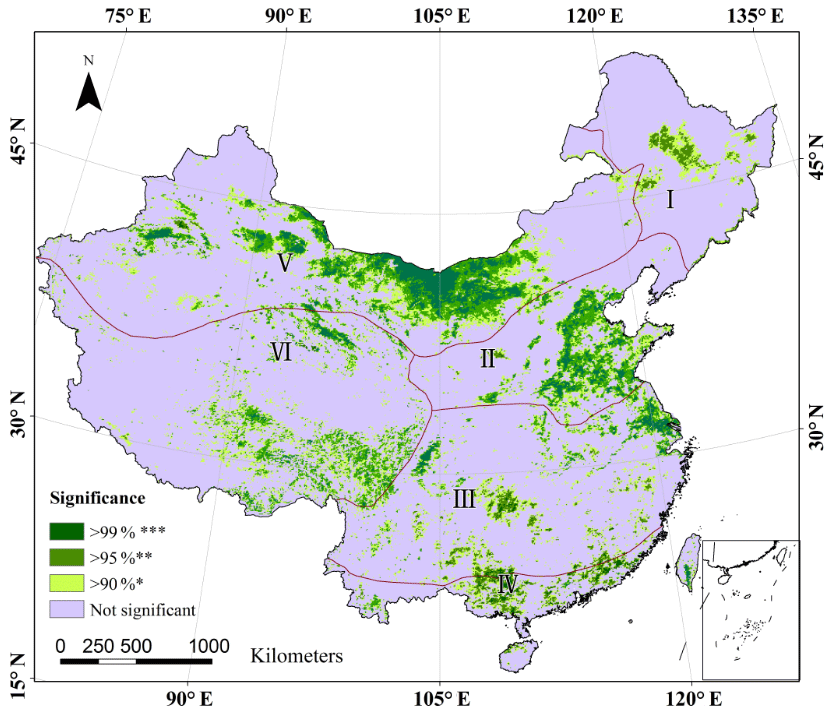
Figure A1 Significance of the spatial distribution of annual average LST trends based on an independent-samples t test in China from 2003 to 2017. Note that the symbols ***, ** and * explain that there are increasing or decreasing tendencies averaged over China at the 99 %, 95 % and 90 % confidence level, respectively (same as Figs. A3 and B2).

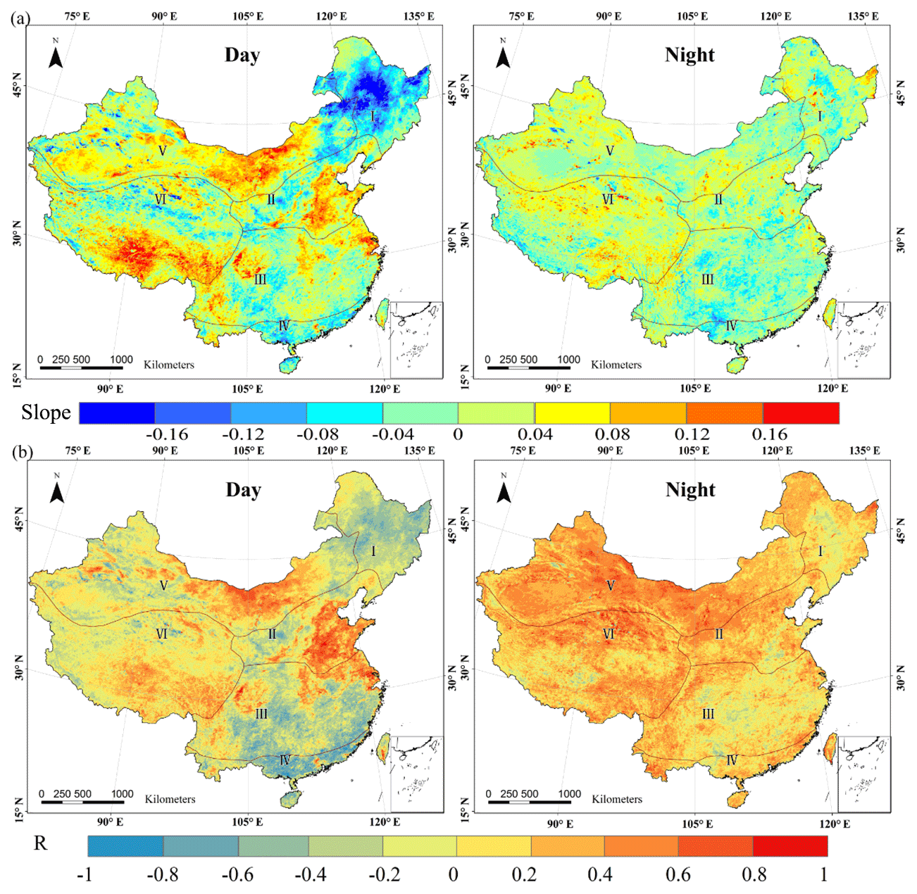
Figure A2 Spatial dynamics of day and night LST change trends based on (a) slope and (b) correlation coefficient.

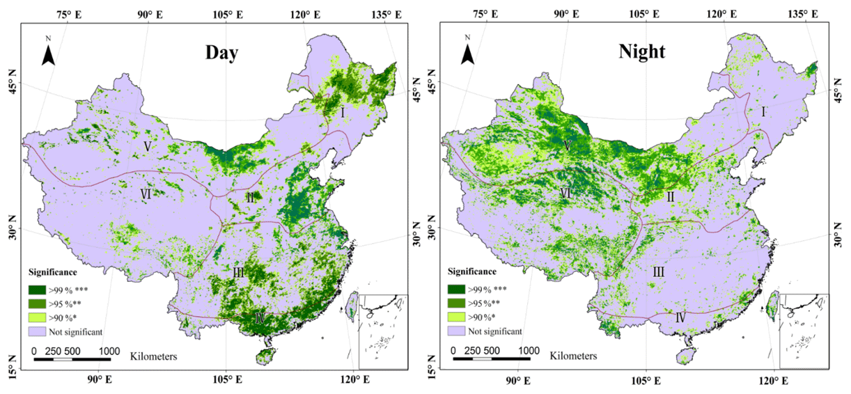
Figure A3 Distribution of diurnal LST change trend significance during 2003–2017.

Appendix B: Seasonal change analysis

In addition to analyzing the characteristics of the interannual variation in LST, we also conducted an analysis of the seasonal variation characteristics to further reveal the LST variation patterns in detail (see Figs. B1 and B2). The variation characteristics are also described by the slope of the change and the correlation coefficient (R) in Sect. 3.4. The results show that there is a significant spatial difference between the seasonal surface temperature trends, reflecting the effect of seasonal temperature changes on regional temperature changes. From 2003 to 2017, the positive trend in the four seasons was most significant in winter, which exhibited the largest warming area (accounting for 70 %), followed by that in spring and summer, and the national average LST change in autumn basically did not change. Compared with the global warming hiatus that occurred from 1998 to 2002, the positive trends in China showed large differences in the four seasons (Li et al., 2015).

Figure B1 The interseasonal variability rates (slope) and correlation coefficients (R) of LST in spring (a), summer (b), autumn (c) and winter (d) from 2003 to 2017: (a1), (b1), (c1) and (d1) are the spatial distributions of the slopes in the four seasons; (a2), (b2), (c2) and (d2) are histograms of the slopes in the four seasons; and (a3), (b3), (c3) and (d3) are the spatial distributions of the correlation coefficients (R) in the four seasons.

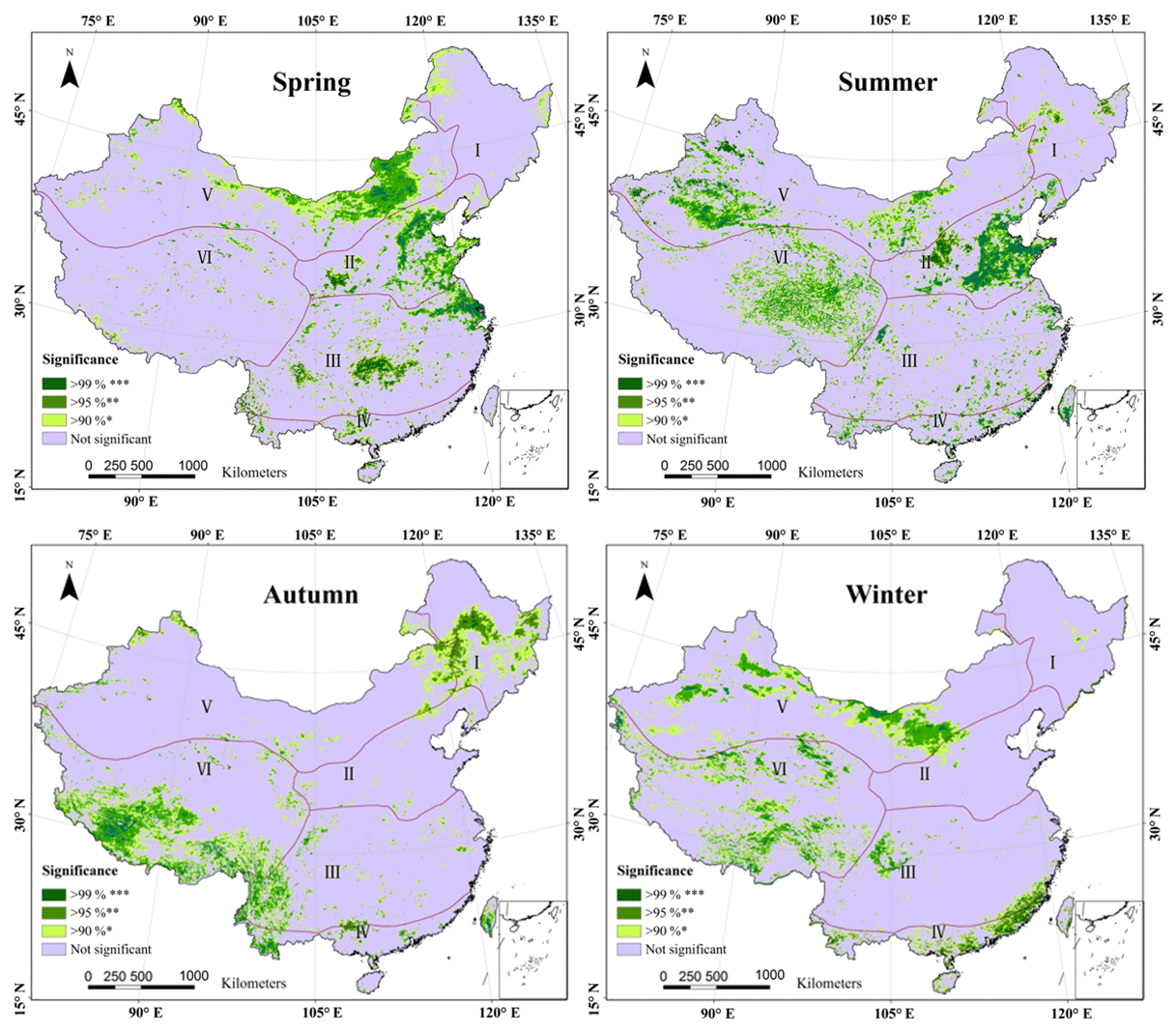
Figure B2 Distribution of seasonal LST trend significance during 2003–2017.

Specifically, in spring, the warming area is mainly concentrated in the northern areas (I, II and V), while a weak negative trend is observed in the southern areas. The largest positive trend over the northern areas appears in the Inner Mongolia Plateau (slope>0.18, P<0.01). In addition, rapid warming also occurred in the North China Plain in the eastern part of the North China Region (II; especially near Beijing and some areas of Hebei Province, slope>0.12, R>0.6, P<0.01).

As shown in Fig. B1, compared with the other two seasons, both summer and autumn showed weak positive trends throughout the country. In summer (Fig. B1, panels b1, b2 and b3), there were slight increasing trends in most areas of China, while there were still negative trends in the Northeast Region (I; details in Fig. B1). Significant increasing trends were mainly observed in the Qinghai–Tibet Plateau, North China Plain, Inner Mongolia Plateau, Tarim Basin and some areas in the north, with the largest positive trend in the Qinghai–Tibet Plateau. In autumn, the negative trends were mainly present in the Northeast Region (I) and the northern Chinese Tian Shan in the Qinghai–Tibet Plateau region (VI). In contrast, the Qinghai–Tibet Plateau was still controlled by strong positive trends (near Lhasa city, slope=0.09, R=0.60, P<0.05), especially in the southern part of the Tanggula Mountains.

Of the areas, 69.4 % experienced warming in winter, which is significantly higher than other seasons (details in Fig. B2). Thus, winter is the most important source of interannual increases in the average LST. The most remarkable positive trends in winter were observed in the Northwest Region (V) and the Qinghai–Tibet Plateau region (VI).