WFDE5: bias-adjusted ERA5 reanalysis data for impact studies

The WFDE5 dataset has been generated using the WATCH Forcing Data (WFD) methodology applied to surface meteorological variables from the ERA5 reanalysis. The WFDEI dataset had previously been generated by applying the WFD methodology to ERA-Interim. The WFDE5 is provided at 0.5^∘ spatial resolution but has higher temporal resolution (hourly) compared to WFDEI (3-hourly). It also has higher spatial variability since it was generated by aggregation of the higher-resolution ERA5 rather than by interpolation of the lower-resolution ERA-Interim data. Evaluation against meteorological observations at 13 globally distributed FLUXNET2015 sites shows that, on average, WFDE5 has lower mean absolute error and higher correlation than WFDEI for all variables. Bias-adjusted monthly precipitation totals of WFDE5 result in more plausible global hydrological water balance components when analysed in an uncalibrated hydrological model (WaterGAP) than with the use of raw ERA5 data for model forcing.

The dataset, which can be downloaded from https://doi.org/10.24381/cds.20d54e34 (C3S, 2020b), is distributed by the Copernicus Climate Change Service (C3S) through its Climate Data Store (CDS, C3S, 2020a) and currently spans from the start of January 1979 to the end of 2018. The dataset has been produced using a number of CDS Toolbox applications, whose source code is available with the data – allowing users to regenerate part of the dataset or apply the same approach to other data. Future updates are expected spanning from 1950 to the most recent year.

A sample of the complete dataset, which covers the whole of the year 2016, is accessible without registration to the CDS at https://doi.org/10.21957/935p-cj60 (Cucchi et al., 2020).

1 Introduction

The development, calibration, and evaluation of impact models require good-quality historical meteorological datasets. These are needed to both drive the impact models themselves and characterize their performances over the historical period. The availability of reliable historical runs is also critical for the preparation of impact studies using climate projections. Reanalyses have long been used for those purposes as they provide a physically consistent global reconstruction of past weather without any gap in space or time. The ERA-Interim global reanalysis for the atmosphere, land surface, and ocean waves (Dee et al., 2011) of the European Centre for Medium Range Weather Forecast (ECMWF) has been used widely as a reference by the climate community. Although reanalyses represent – by construction – the most plausible state of the atmosphere and the ocean given the observations and the forecasts from the model at a previous time-step, the coarse resolutions of models, the assumptions made in sub-grid parameterizations, and, more generally, the overall inadequacies of the modelling framework are known to induce biases with respect to ground-based observations and radiosondes. Considering that the primary goal of impact studies is to assess the climate change impacts in the real world (opposite to the modelled world), it is essential that such biases are first characterized and then, as much as practically possible, corrected for.

Recently the ERA5 reanalysis has superseded the ERA-Interim reanalysis (Hersbach et al., 2020). It is produced at ECMWF as part of the EU-funded Copernicus Climate Change Service (C3S). At the time of writing, data were available from the C3S Climate Data Store (CDS) for the period from 1979 onwards. Timely updates are provided with a 5 d latency, while a more thorough quality check is provided 2–3 months later. In 2020 the dataset will be extended back to 1950 and will then also encompass the period covered by ERA-40 (1957–2002; Uppala et al., 2005). ERA5 is based on 4D-Var data assimilation using Cycle 41r2 of the Integrated Forecasting System (IFS), which was operational at ECMWF in 2016. As such, compared to ERA-Interim (which was based on an IFS cycle that dates from 2006), ERA5 benefits from a decade of developments in model physics, core dynamics, and data assimilation. In addition to a significantly enhanced horizontal resolution (31 km grid spacing compared to 80 km for ERA-Interim), ERA5 has a number of innovative features. These include hourly output throughout and an uncertainty estimate. The uncertainty information is obtained from a 10-member ensemble of data assimilations with 3-hourly output at half the horizontal resolution (63 km grid spacing). Compared to ERA-Interim, ERA5 also provides an enhanced number of output parameters. An overview of the main characteristics and general performance of ERA5 and a comparison with ERA-Interim is provided in Hersbach et al. (2020), while more in-depth studies of particular aspects have been reported in a growing number of publications in the scientific literature.

The move from ERA-Interim to ERA5 represents a step change in overall quality and level of detail, whose increase has been reported in a large number of publications. Several of these have been summarized in Hersbach et al. (2020), and the benefit of hourly resolution is illustrated for the December 1999 storm Lothar in that paper as well. Hersbach et al. (2019) shows the increased level in detail of precipitation over the North Atlantic.

ERA5 utilizes a vast amount of synoptic observations. The number has increased from approximately 0.75 million per day on average in 1979 to around 24 million per day by the end of 2018. Satellite radiances are the dominant and growing type of data throughout the period. The volume of conventional data has also increased steadily. In addition to observations, ERA5 relies on gridded information about radiative forcing and boundary conditions. For radiation, ERA5 includes forcings for total solar irradiance, ozone, greenhouse gases, and some aerosols developed for the World Climate Research Programme (WCRP) Coupled Model Intercomparison Project Phase 5 (CMIP5) initiative, including stratospheric sulfate aerosols. This represents a major improvement on ERA-Interim, which, for example, does not account for stratospheric sulfate aerosols due to major volcanic eruptions. Details are provided in Hersbach et al. (2015). The evolution of sea-surface temperature (SST) and sea ice cover is based on a combination of products: the UK Met Office Hadley Centre HadISST2 product for SST, the EUMETSAT OSI-SAF reprocessed product for sea ice, and the UK Met Office OSTIA product for SST and sea ice that is also used in ECMWF’s operational forecasting system. Details can be found in Hirahara et al. (2016).

Table 1 Sources of data used to derive the WFDE5 dataset

The EU WATCH programme produced a common framework for land surface models (LSMs) and global hydrological models (GHMs) to assess the global terrestrial hydrological cycle in the 20th and 21st centuries. This required a common meteorological forcing dataset for the 20th century, which became the WATCH Forcing Data (WFD). The WFD, based on the ERA40 reanalysis, allowed intercomparisons of hydrological models and bias correction of 21st century GCM outputs (Haddeland et al., 2011; Hagemann et al., 2011). The modelling in WATCH required sub-daily and daily average data at half-degree spatial resolution, necessitating interpolation onto the regular latitude–longitude grid, land–sea mask, and elevations used by the Climate Research Unit (CRU). The WFD methodology (Weedon et al., 2010, 2011) involved common processing of all terrestrial half-degree grid boxes outside Antarctica at 3-hourly steps, with elevation correction of air temperature and consequent adjustment of surface pressure, specific humidity, and downwards longwave radiation. Bias correction utilized the CRU gridded observations (New et al., 1999, 2000) of monthly average air temperature, diurnal temperature range, cloud cover (for adjusting average downwards shortwave fluxes), precipitation totals, and number of “wet” (i.e. precipitation) days. Additionally, downwards shortwave radiation was corrected for changes in multi-year tropospheric and stratospheric aerosol loading. Unlike most other reanalyses, ERA provides rainfall and snowfall rates separately, and this permitted adjustment of these rates to allow for the precipitation gauge catch corrections inherent in the observed CRU precipitation totals. Though critical for hydrological modelling, the precipitation variables are the least well constrained by surface observations, so data were provided in two versions dependent on the source of the gridded monthly observed precipitation totals – one based on CRU and the other on the “full data product” of the Global Precipitation Climatology Centre (GPCC).

Later, the WFD methodology was applied to the ERA-Interim reanalysis (Dee et al., 2011) to produce the WFDEI dataset (Weedon et al., 2014). As before, the reanalysis data were 3-hourly and interpolated onto the CRU land–sea mask. Unlike the WFD, the WFDEI includes Antarctica, and an extra processing step was introduced for the precipitation variables after correction of monthly totals and numbers of wet days and before correction of precipitation gauge biases. This involved overriding the reanalysis ratio of rainfall to snowfall in each time step in cases where the differences between the CRU grid box elevation differed substantially from ERA-Interim elevation (Weedon et al., 2014). Intermittent updates of the WFDEI beyond 2009 used the latest versions of CRU and GPCC – i.e. WFDEI files for additional years were added rather than entire new versions of the files created.

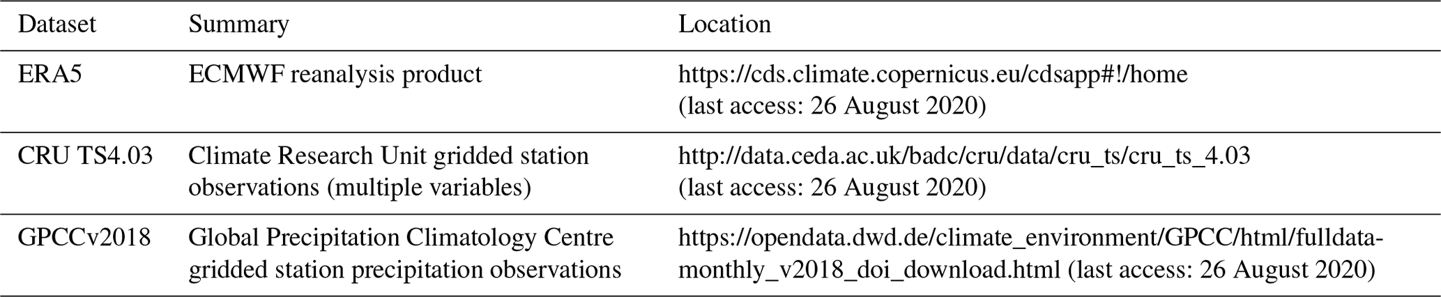
Here we describe the WFDE5 (i.e. “WATCH Forcing Data methodology applied to ERA5 reanalysis data”, C3S, 2020b), a new meteorological forcing dataset for land surface and hydrological models based on the ERA5 reanalysis (Copernicus Climate Change Service, 2017). It consists of 11 variables (see Table 2) with an hourly temporal resolution on a regular longitude–latitude half-degree grid, with global spatial coverage and values defined only for land and lake points. The dataset was derived by applying the sequential elevation and monthly bias correction methods described in Weedon et al. (2010, 2011) to half-degree aggregated ERA5 reanalysis products. The monthly observational datasets used for bias correction are CRU TS4.03 from CRU (Harris et al., 2020) for 1979 to 2018 for all variables and the GPCCv2018 full data product (Schneider et al., 2018) for rainfall and snowfall rates for 1979 to 2016. In addition, as described below, the aerosol correction step for shortwave radiation has been revised with respect to WFD and WFDEI. For an outline of the methodology applied and a reference to the observation datasets used, see Tables 1 and 2.

Table 2 WFDE5 elevation and bias correction methodology outline (Weedon et al., 2010, 2011).

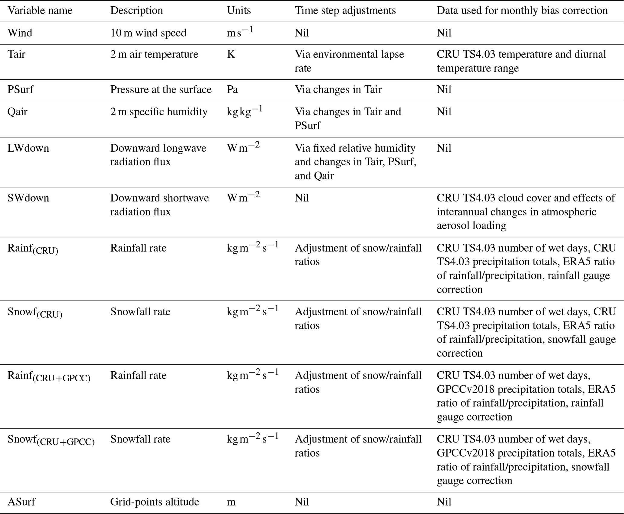
Variable names and units are based on the ALMA (Assistance for Land-‐surface Modelling Activities) conventions (https://www.lmd.jussieu.fr/~polcher/ALMA/, last access: 26 August 2020). Wind, Tair, PSurf, and Qair variables have instantaneous values, while LWdown, SWdown, Rainf, and Snowf are averaged over the next hour at each date and time.

As a meteorological forcing dataset, WFDE5 facilitates climate impact simulations such as those carried out in the Inter-Sectoral Impact Model Intercomparison Project (ISIMIP; Warszawski et al., 2014; Frieler et al., 2017). It can be used to directly drive historical impact simulations, which are needed for impact model validation. It can also be used as an observational reference dataset for the bias adjustment of future climate projections; these bias-adjusted climate projections can then be used to drive future climate impact projections. Both predecessors of WFDE5 have been employed for these two purposes in previous ISIMIP phases. In particular, the bias adjustment of future climate projections was done using the WFD in the ISIMIP Fast Track (Hempel et al., 2013) and the EartH2Observe, WFDEI, and ERA-Interim data merged and bias-corrected for ISIMIP (EWEMBI; Lange, 2018, 2019a) in ISIMIP2b (Frieler et al., 2017). WFDE5 will be similarly employed in the upcoming ISIMIP phase 3.

2 Dataset Processing

All computations were carried out within the CDS Toolbox, a python coding environment to retrieve, process, plot, and download data from the C3S Climate Data Store (CDS, C3S, 2020a). The CDS Toolbox scripts used to generate the dataset are publicly available at https://doi.org/10.24381/cds.20d54e34 under a free and open licence and can be used to reproduce the dataset.

2.1 Extraction and aggregation of reanalysis data

ERA5 reanalysis data are available in the CDS on regular latitude–longitude grids at $\mathrm{0.25}{}^{\circ }\times \mathrm{0.25}{}^{\circ }$, as a result of finite-element-based linear interpolation from the original reduced Gaussian grid at ∼ 0.28^∘, and atmospheric parameters are distributed on 37 pressure levels. They are distributed at hourly resolution, and the date and time to which each value refers to is represented using the validity date and time: for instantaneous variables, it corresponds to the date and time at which each value is considered valid; for accumulated variables, it represents the ending date and time of the interval over which the variable is accumulated, and hence over which each value can be considered valid. Accumulation variables are aggregated over the hour ending at the validity date and time, and they are automatically converted to mean rates when retrieved from within the CDS Toolbox.

Before applying elevation and bias correction, two preprocessing steps were performed on ERA5 reanalysis data. First, in order to enable comparison and bias correction using the CRU dataset, ERA5 reanalysis were regridded to regular half-degree longitude–latitude grid, via first-order conservative remapping (Jones, 1999). Then, a backward 1 h time shift was applied to rate variables, so that values stored at each date–time represents time averages over the following hour. The latter step was taken in order to adhere to the scheme used for the WATCH Forcing Dataset (Weedon et al., 2011).

It is worth noticing that grid-points classified as belonging to land in CRU TS4.03 and GPCCv2018 datasets are not necessarily classified as land-points in ERA5 reanalysis dataset. This is especially true for coastal grid-points, for which not considering this issue often led to anomalous values in the first iteration of the WFDE5 dataset. For this reason, besides applying CRU TS4.03/GPCCv2018 to ERA5 reanalysis after half-degree regridding, an additional mask derived by ERA5 quarter-degree land–sea and lake cover mask is applied just after retrieval. In this way, the final WFDE5 dataset contains values only for grid-points that are classified as land or lake by both ERA5 and CRU.

2.2 Elevation and bias correction

Once aggregation had been performed, the sequential elevation and monthly bias correction methods of Weedon et al. (2010, 2011) were applied to the regridded data (see Table 2). The same procedures used for the creation of the WFDEI (Weedon et al., 2014) were applied, with the only exception of near-surface specific humidity (Qair). For this variable, given the absence of both ERA5 near-surface specific and relative humidity from the CDS, a slightly different approach was taken: first, ERA5 vapour pressure and saturation vapour pressure at the surface, e and e_sat, respectively, were computed following Buck (1981). Following this, they were used to compute ERA5 relative humidity at surface as $\text{RH}=\mathrm{100.0}\cdot e/e_{\text{sat}}$; finally, at this point, the algorithm described in Weedon et al. (2010) could be resumed.

Likewise for the WFD (Weedon et al., 2011) and WFDEI (Weedon et al., 2014) datasets, downward shortwave radiation was adjusted at the monthly timescale using CRU cloud cover and the local linear correlation between monthly average (aggregated) ERA5 cloud cover and downward shortwave radiation (Sheffield et al., 2006; Weedon et al., 2010).

ERA5 includes a simplified representation of the time evolution of sulfate aerosols, which interact with radiation only in that model, but otherwise does not account for the impact on surface radiative fluxes of changes in aerosol interactions with radiation (also called direct effects of aerosols) and clouds (also called first indirect effects of aerosols). To represent those impacts, aerosol corrections are calculated as monthly distributions of the anomaly in downward surface shortwave radiative flux due to aerosol–radiation and aerosol–cloud interactions over the period 1979–2018. Radiative transfer calculations, which use the tools described in Sect. 2.f.ii of Weedon et al. (2010), are based on monthly averaged distributions of tropospheric and stratospheric aerosol optical depth and cloud fraction. The time series of tropospheric optical depth for sulfate, fossil-fuel black and organic carbon, biomass burning, mineral dust, sea salt, and secondary biogenic aerosols is taken from the historical and RCP8.5 simulations by the HadGEM2-ES climate model (Bellouin et al., 2011). To correct for biases in HadGEM2-ES aerosol optical depths, these optical depths are scaled over the whole period and for each aerosol species to match the global and monthly averages obtained by the CAMS Reanalysis of atmospheric composition (2003–2017; Inness et al., 2019), which assimilates satellite retrievals of aerosol optical depth. This bias correction was not applied in WFD and WFDEI but is now possible thanks to the availability of the CAMS Reanalysis. The time series of stratospheric aerosol optical depth is taken from the climatology by Sato et al. (1993), which has been updated to 2012 at https://data.giss.nasa.gov/modelforce/strataer/ (last access: 26 August 2020). The years 2013–2017 are assumed to match background years, thus they replicate year 2010. That assumption is supported by the Global Space-based Stratospheric Aerosol Climatology time series (1979–2016; Thomason et al., 2018). The time series of cloud fraction is taken from CRU TS 4.03, for consistency with other aspects of the WFDE5 dataset. Surface radiative fluxes account for aerosol–radiation interactions from both tropospheric and stratospheric aerosols and for aerosol–cloud interactions from tropospheric aerosols except mineral dust. The radiative effects of aerosol–cloud interactions are assumed to scale with the radiative effects of aerosol–radiation interactions using regional scaling factors derived from HadGEM2-ES. To avoid double-counting the radiative effects of aerosol–radiation interactions by sulfate aerosols, which are to some extent already represented in ERA5, the radiative transfer calculations are repeated, this time only including sulfate aerosol–radiation interactions and the corresponding anomalies subtracted from the set of fluxes obtained previously. Atmospheric constituents other than aerosols and clouds are set to a constant standard mid-latitude summer atmosphere because their variations only have second-order effects on aerosol corrections.

Table 3 Summary of WFDE5 dataset attributes on the C3S Climate Data Store.

Finally, similarly to the WFD and WFDEI datasets, two different WFDE5 rainfall and snowfall rates datasets, including gauge catch corrections, were generated by using either CRU TS4.03 or GPCCv2018 precipitation totals. The GPCCv2018 database includes around 3–4 times as many precipitation stations as CRU (incorporating most of the latter as a subset, Becker et al., 2013; Schneider et al., 2014) but extends only till 2016. As already pointed out in Weedon et al. (2014), during generation of the WFDE5 precipitation rates an error in the precipitation phase can arise locally where there are large elevation differences between ERA5 and CRU grids. For this reason, a further processing step was added to the WFD methodology to correct the most extreme cases of inappropriate precipitation phase: for each grid box and each calendar month over 1979–2018, records of the minimum Tair during rainfall and the maximum Tair during snowfall (“phase temperature extremes”) were stored; then, for each grid box and hourly time step, the precipitation phase was switched if the combination of the phase with the elevation and bias-corrected Tair were beyond a phase temperature extreme.

Elevation and bias correction was applied for all land points outside Antarctica. For grid points belonging to this region, given the absence of observational data, only elevation correction was applied.

2.3 Higher resolution WFDE5 data

The WFDE5 has been provided at $\mathrm{0.5}{}^{\circ }\times \mathrm{0.5}{}^{\circ }$ resolution rather than at $\mathrm{0.25}{}^{\circ }\times \mathrm{0.25}{}^{\circ }$ as in the original ERA5 data. There are several reasons for this. The project to generate WFDE5 was also designed to deliver open-source software so that users could regenerate the data at the original or, eventually, higher resolution. Three main considerations influenced the initial generation of the WFDE5 dataset:

1. the need to generate data in time for ISIMIP3 and their reporting to the AR6 of IPCC in 2020,

2. the need to convert the existing WFDEI Fortran programs into CDS Toolbox workflows and easily test the output,

3. the requirement for appropriate and freely available global land-gridded observations for bias correction.

The first consideration meant that any procedures adopted had to be practical and fast. The simplest way to test whether the CDS Toolbox workflows were working was to apply them to ERA-Interim data and check that they correctly reproduced the WFDEI data. This implied generating output at the same resolution as the WFDEI and CRU. Additionally, ISIMIP3 only required data at $\mathrm{0.5}{}^{\circ }\times \mathrm{0.5}{}^{\circ }$ since their models were set up at that resolution.

The WFDE5 CDS workflows will eventually allow users to generate higher resolution data on their own. At the moment, this can only be done using interpolated CRU TS4.03 and GPCCv2018 datasets, copies of which are hosted on a dedicated CDS machine and made accessible through the CDS Toolbox. Another option would be to use higher-resolution observational datasets, such as quarter-degree GPCC or MSWEP (Beck et al., 2017, 2019b) for total precipitation. This option will be viable once additional datasets can be hosted on the C3S Climate Data Store.

3 Data and software access

The WFDE5 dataset is distributed by the Copernicus Climate Change Service (C3S) through its Climate Data Store (CDS) as monthly files in NetCDF format and can be downloaded at https://doi.org/10.24381/cds.20d54e34 (C3S, 2020b). It uses a full half‐degree grid (720×360 grid boxes) with the sea and large lakes flagged as missing data, comprising a total of 92889 land points (Antarctica included). General dataset attributes are described in Table 3. A sample of the complete dataset, which covers the whole of the year 2016, is accessible without registration to the CDS at https://doi.org/10.21957/935p-cj60 (Cucchi et al., 2020).

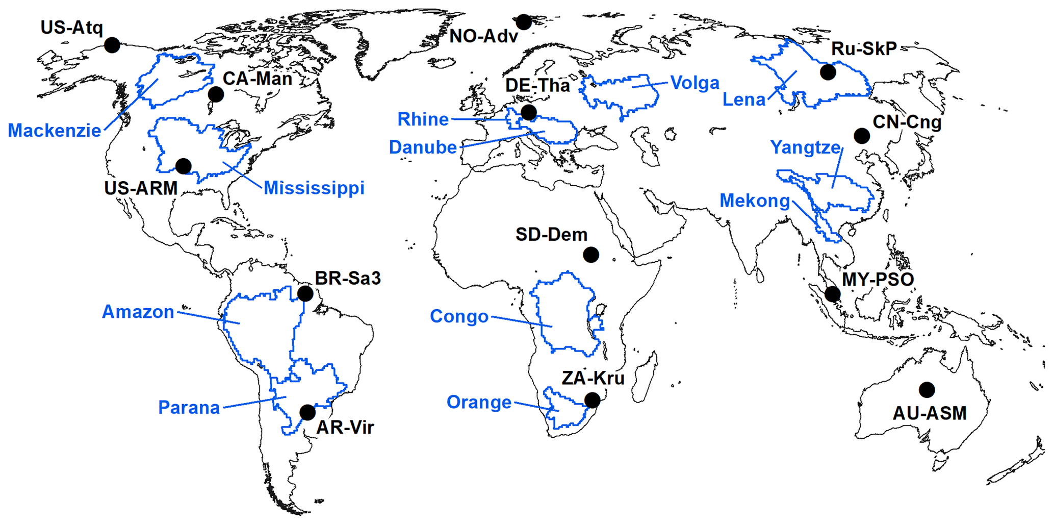
Figure 1 Location of FLUXNET2015 sites used to evaluate ERA5, WFDE5, and WFDEI, as well as river basin outlines for the hydrological assessment.

All the CDS Toolbox workflows used to generate WFDE5 are publicly available (https://doi.org/10.24381/cds.20d54e34) and can be used to regenerate samples of the dataset. Furthermore, as ERA5 progresses, using these applications it will be possible to expand WFDE5 dataset back to the start of 1950 and forward beyond 2018.

4 Evaluation

4.1 Previous analyses

Beck et al. (2019a) assessed multiple precipitation datasets at daily time steps against radar and precipitation gauge observations across the contiguous USA. Their analysis included ERA5, ERA-Interim and WFDEI precipitation adjusted to GPCC totals. They demonstrated that against observations ERA5 precipitation provides a significant improvement over both ERA-Interim and WFDEI precipitation. Albergel et al. (2018) used the ISBA LSM to assess the use of ERA5 versus ERA-Interim forcing. They assessed performance against a wide variety of observed hydrological and vegetation-related variables. Significant improvements were demonstrated in the simulation of the hydrological cycle using ERA5, which they mostly attributed to better precipitation. There were small changes related to vegetation modelling. For a region with a low density of gauges in Iran, Fallah et al. (2020) showed that ERA5 precipitation is closer to local observations than ERA-Interim but that GPCCv2018 (used here in bias correction or ERA5) is substantially better.

4.2 Comparison with FLUXNET2015 and WFDEI

The FLUXNET2015 (FN2015) meteorological data (Chu, 2015; Pastorello et al., 2017) are not included in the data assimilation of the ERA5 reanalysis. Therefore, these data provide an opportunity to assess the degree to which the ERA5 and WFDE5 meteorological variables agree with surface observations. Despite there being over 200 FN2015 sites globally, they are highly clustered within Europe and North America. In order to provide a fairly uniform global assessment, 13 sites with at least 3 years of data have been selected from 12 countries spanning a wide range of longitudes and latitudes (Fig. 1, Table 4). The primary purpose of the FN2015 meteorological dataset is to provide data for forcing LSMs to allow comparison with the FN2015 surface exchange fluxes of energy and carbon. As such, the FN2015 meteorological variables have been gap-filled using ERA-Interim data to allow modelling without missing data. To avoid biasing the comparisons made here, only meteorological values that are measurements have been used (i.e. at times and locations where the FN2015 tier 1 quality flag is 0). Unfortunately, this means that some FN2015 sites do not provide observations for some variables at any time step (“missing variables” in Table 4).

Table 4 Selected FLUXNET2015 sites.

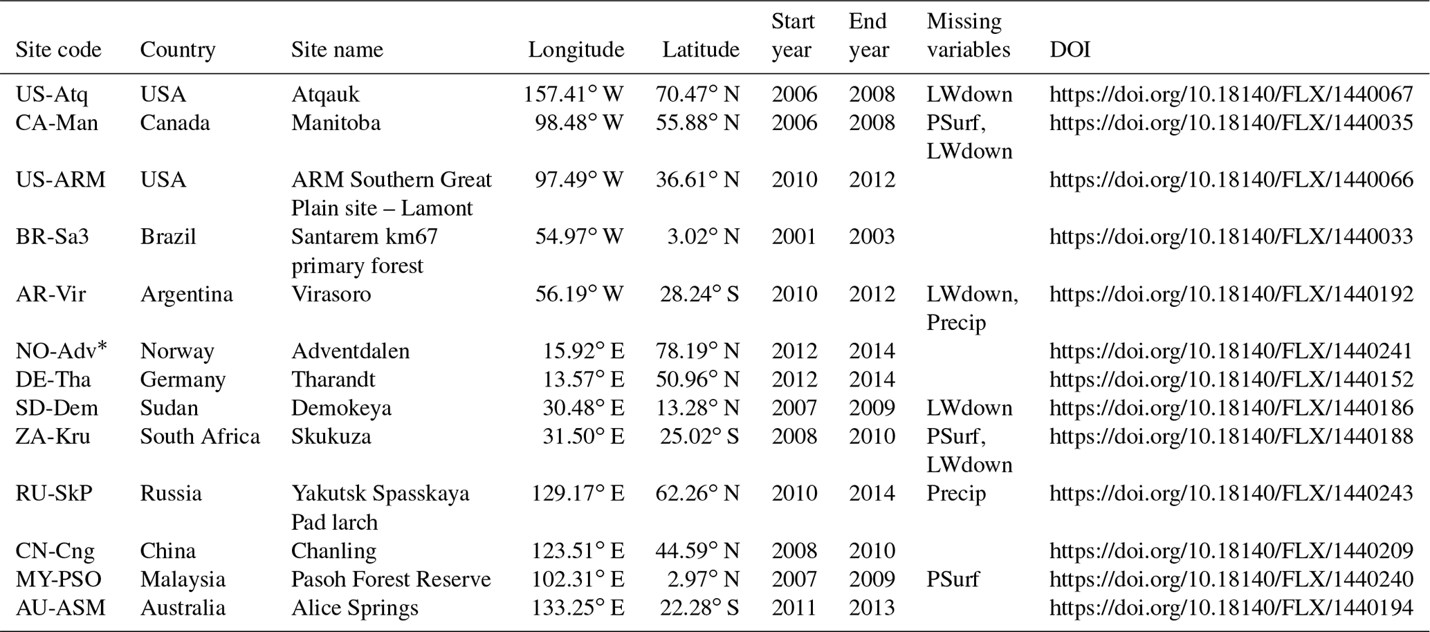
^* NO-Adv is now designated as SL-Adv (i.e. within Svalbard). Precip stands for precipitation. Note that “missing variables” refers to tier 1 items provided by FLUXNET2015 as entirely gap-filled, i.e. not measured, values.

Two pairs of comparisons have been made: firstly for ERA5 (aggregated to half degree) versus FN2015, as well as for WFDE5 versus FN2015 at an hourly time step. This required converting the half-hourly FN2015 data to hourly steps and aligning the time stamps since ERA5 is based on UTC instead of local time. ERA5 does not provide specific humidity so Qair was calculated using the 2 m air temperature, surface pressure, and relative humidity using equations 4 and 6 of Buck (1981). The second comparisons were for WFDEI versus FN2015 and for WFDE5 versus FN2015 at 3-hourly time steps, again with alignment of time stamps. At each site mean bias error (MBE), mean absolute error (MAE), and correlation were calculated. MAE was used instead of root-mean-square error since the former provides a less ambiguous basis for assessment (Willmott and Matsuura, 2005). Since the data are time series there is considerable serial correlation leading to spuriously high values. Consequently, the correlations of the previously pre-whitened time series – i.e. adjusted to remove lag-1 autocorrelation – are also reported as “adjusted correlation” (Ebisuzaki, 1997). Data for individual sites are reported for ERA5 and WFDE5 versus FN2015 (hourly) in Tables A1–A8 and for WFDEI and WFDE5 versus FN2015 (3-hourly) in Tables A9–A16. Average metrics for the pairs of comparisons are shown in Fig. 2 and Tables A17 and A18.

Figure 2 Average metrics (mean ± 95 % confidence interval of the mean) for (a) ERA5 versus FN2015 (blue) and WFDE5 versus FN2015 (red) at hourly time steps (see Table A17); (b) WFDEI versus FN2015 (blue) and WFDE5 versus FN2015 (red) at three-hourly time steps (see Table A18).

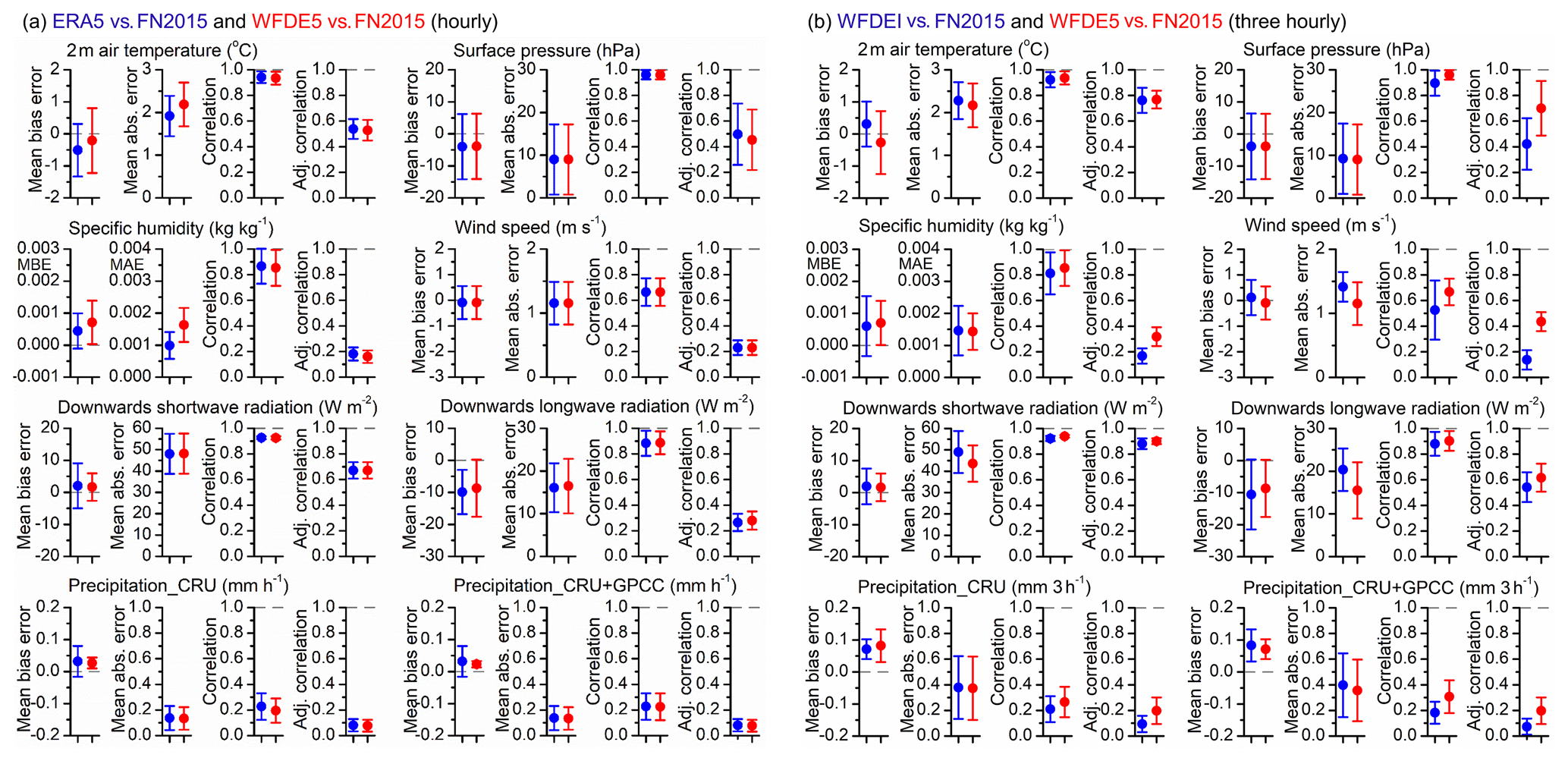
At hourly steps on average there are no significant differences in MBE, MAE, correlation or adjusted correlation between ERA5 versus FN2015 and WFDE5 versus FN2015, for all variables apart from two (Fig. 2a). For air temperature the MBE is slightly better (closer to zero) for WFDE5, whereas the MAE is slightly worse (larger) for WFDE5. On the other hand, for specific humidity both the MBE and MAE are slightly worse for WFDE5. These results indicate that the bias and elevation corrections incorporated into the WFDE5 have had little overall effect on the performance against surface observations compared to ERA5.

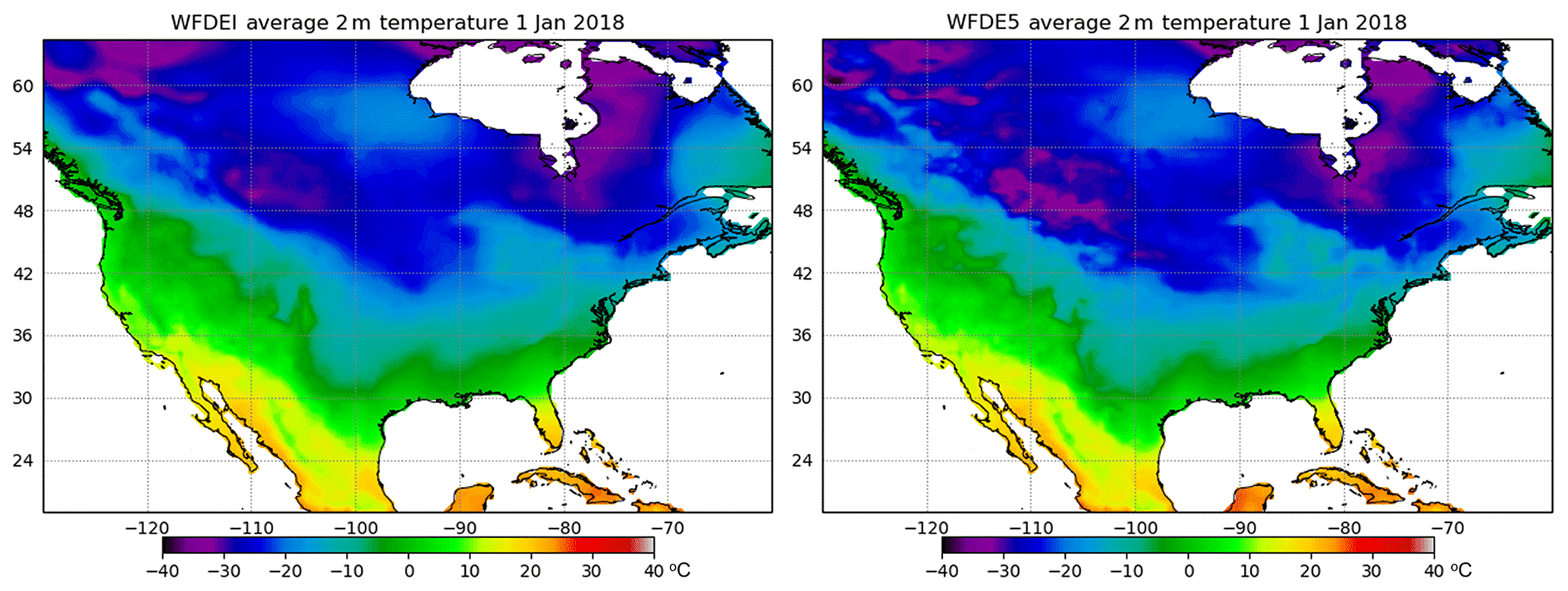
Figure 3 Average 2 m temperature on 1 January 2018 for north and central America.

At three hourly steps, for all variables apart from precipitation, the average MBE plus 95 % confidence intervals overlap zero for WFDEI and WFDE5 (Fig. 2b). For wind speed, downwards longwave and downwards shortwave the MAE is slightly better (smaller) for WFDE5 than WFDEI. For all variables aside from precipitation, the MAE, correlation, and adjusted correlation are slightly better for WFDE5 than WFDEI. For precipitation the MBE is slightly better and the correlation slightly higher for WFDE5 versus WFDEI when corrected using the GPCC-corrected, rather than CRU-corrected, precipitation totals. These results indicate that, on average, at the FN2015 sites selected, WFDE5 performs better than WFDEI against the observations. Note that the average results in Fig. 2b and Table A17 hide the fact that for all metrics WFDEI data provide better results (MBE closer to 0.0, MAE lower, correlation higher) for some individual sites than WFDE5 (Tables A9–A16). On the other hand, for wind (speed) and precipitation (CRU- and GPCC-corrected) the correlation and adjusted correlation are better for WFDE5 than WFDEI at every site.

Both WFDEI and WFDE5 in 2017 and 2018 are corrected using CRU TS4.03, so at monthly scales and longer there will be only small differences. However, at sub-monthly timescales, aside from advances in the processing system between the reanalyses used, it is likely that the better performance of WFDE5 is linked to superior spatial variability of ERA5 (data aggregated for WFDE5) versus ERA-Interim (data interpolated for WFDEI). This can be seen in the higher-resolution features of daily average temperature for a single day in January 2018 in North America and Central America in the WFDE5 data (Fig. 3).

4.3 Validation with a global hydrological model

Of great importance for driving impact models such as global hydrological models is the climate forcing input, since the water balance components are highly dependent on it (Müller Schmied et al., 2016). In order to test WFDE5 in terms of suitability for use with an impact model, the global water availability and water use model WaterGAP (version 2.2c, Müller Schmied et al., 2016) was used. WaterGAP calculates water storages and fluxes on global land area (except Antarctica) on a $\mathrm{0.5}{}^{\circ }\times \mathrm{0.5}{}^{\circ }$ resolution (55×55 km at the Equator) and incorporates human interventions such as human water use and man-made reservoirs. Forcing requirements are daily values for precipitation (sum of rainfall and snowfall), average temperature, downwards shortwave radiation, and downwards longwave radiation. For model-specific details, the reader is referred to Müller Schmied et al. (2016, 2014), and Döll et al. (2003). Despite the possibility of calibrating the model, WaterGAP was run with an uncalibrated setup (model parameter γ set to 2, whereas CFA and CFS are set to 1 globally; details can be found in Müller Schmied et al., 2014). This parameter choice was designated to mimic the behaviour in a typical impact model and also due to time and technical constraints (a time series start year of 1920 or earlier is required for standard calibration). The model was driven by ERA5, WFDE5, and WFDEI (the latter two with monthly precipitation scaled to both GPCC and CRU) and was assessed in terms of resulting water balance components (Table 5), model efficiency (Fig. 4), and river discharge seasonality for selected large river basins (Fig. 5).

Table 5 Long-term-annual water balance components [km³ yr⁻¹] as simulated with uncalibrated WaterGAP 2.2c for 1981–2010 and for global land area (except Antarctica and Greenland).

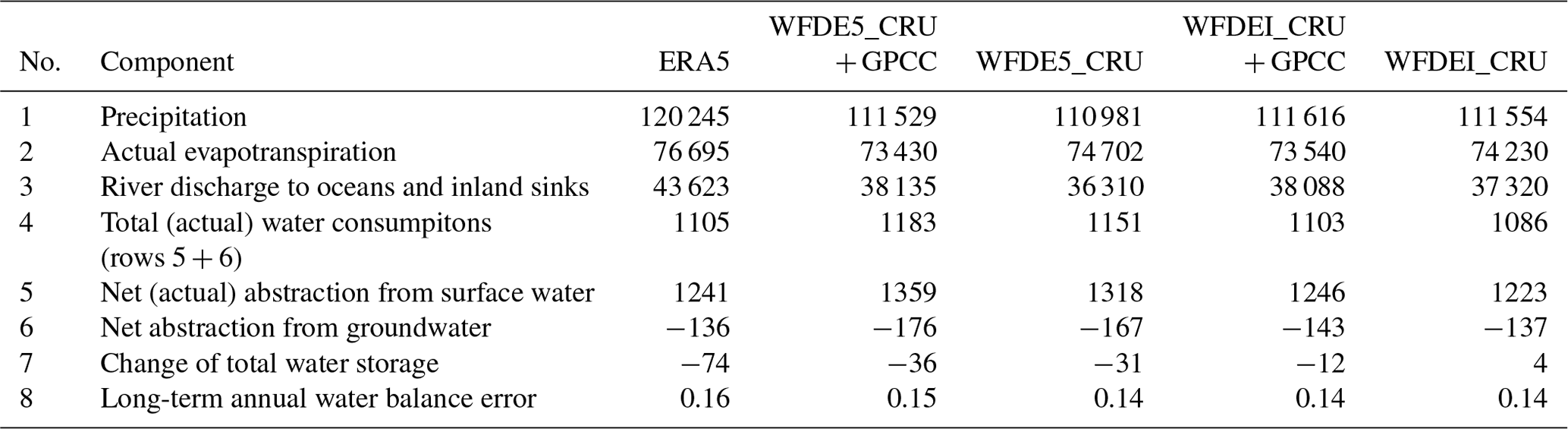
The long-term-annual water balance shows considerably (around 10 %) higher precipitation (P) for ERA5 compared to the WFDE5 adjustments to GPCC or CRU which results in higher values for actual evapotranspiration (AET) and greater river discharge to oceans and inland sinks (Q) (Table 5). The general reduction of mean global precipitation from 120 000 km³ yr⁻¹ for ERA5 to observation-based datasets with around 111 000 km³ yr⁻¹ for WFDE5 is consistent with previous estimates (109 631 to 111 050 km³ yr⁻¹ for the time span 1971–2000 for the snow-undercatch-corrected climate forcings in Tables 3 and 4 of Müller Schmied et al., 2016). Even though WaterGAP was not calibrated, AET and Q are well within the estimates of other models or datasets (AET 62 800–75 981 km³ yr⁻¹ and Q 34 400–44 560 for most assessments according to Müller Schmied et al., 2014, Table 5). The differences in GPCC and CRU dataset versions to adjust ERA5 (ERA-Interim) precipitation for WFDE5 (WFDEI) is substantially smaller for GPCC (precipitation difference: 87 km³ yr⁻¹ for WFDE5_CRU+GPCC versus WFDEI_CRU+GPCC) compared to CRU (precipitation difference: 573 km³ yr⁻¹ for WFDE5_CRU versus WFDEI_CRU). Consequently, differences in simulated river discharge are higher for WFDE5_CRU versus WFDEI_CRU (1010 km³ yr⁻¹) compared to WFDE5_CRU+GPCC versus WFDEI_CRU+GPCC (47 km³ yr⁻¹). This implies that the choice of precipitation bias adjustment target (CRU or GPCC) impacts water balance components.

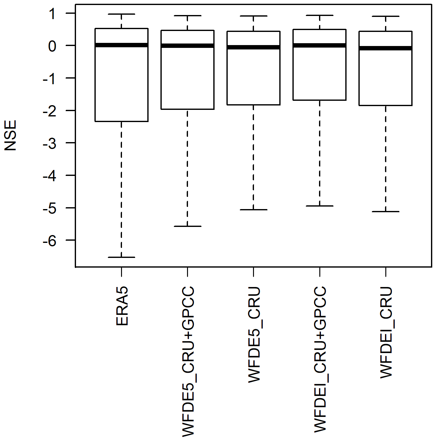
Figure 4 Model efficiency for the uncalibrated runs of the climate forcings in this assessment using monthly time series of 1216 GRDC stations.

The performance of the uncalibrated model runs have been assessed using the widely used Nash–Sutcliffe efficiency metric (NSE, Nash and Sutcliffe, 1970) relative to monthly time series of GRDC station observed discharge. A total of 1216 stations have been used out of the usual 1319 stations used for WaterGAP calibration (Müller Schmied et al., 2014) constrained by data availability for at least 1 year in the time span of the forcing. The optimum NSE is 1, and the value can become infinitely negative, but below 0 the simulation is not better than the average of the observations (Nash and Sutcliffe, 1970). The median performances of the model runs are similar and around the value 0, with some ranging towards optimum but also towards negative NSE values. Note that around 16 % to 17 % of the stations are consistently outside of the limits of the boxplots (NSE > 1.5 × inter quartile range) towards negative values and not displayed. Generally, the variants scaled to GPCC tend to have a slightly better performance than the values scaled to CRU. Typically, the performance increases as a result of calibrating the model (see Müller Schmied et al., 2014, Fig. 6), so the NSE values reported here should not be wrongly interpreted as the result of the poor quality of the forcing data but more in the sense of that uncalibrated impact models could reach – in principle – similar efficiencies independently of the forcing data assessed here (with slight advantages of the bias-adjusted WFDE5 data compared to direct use of ERA5, Fig. 4).

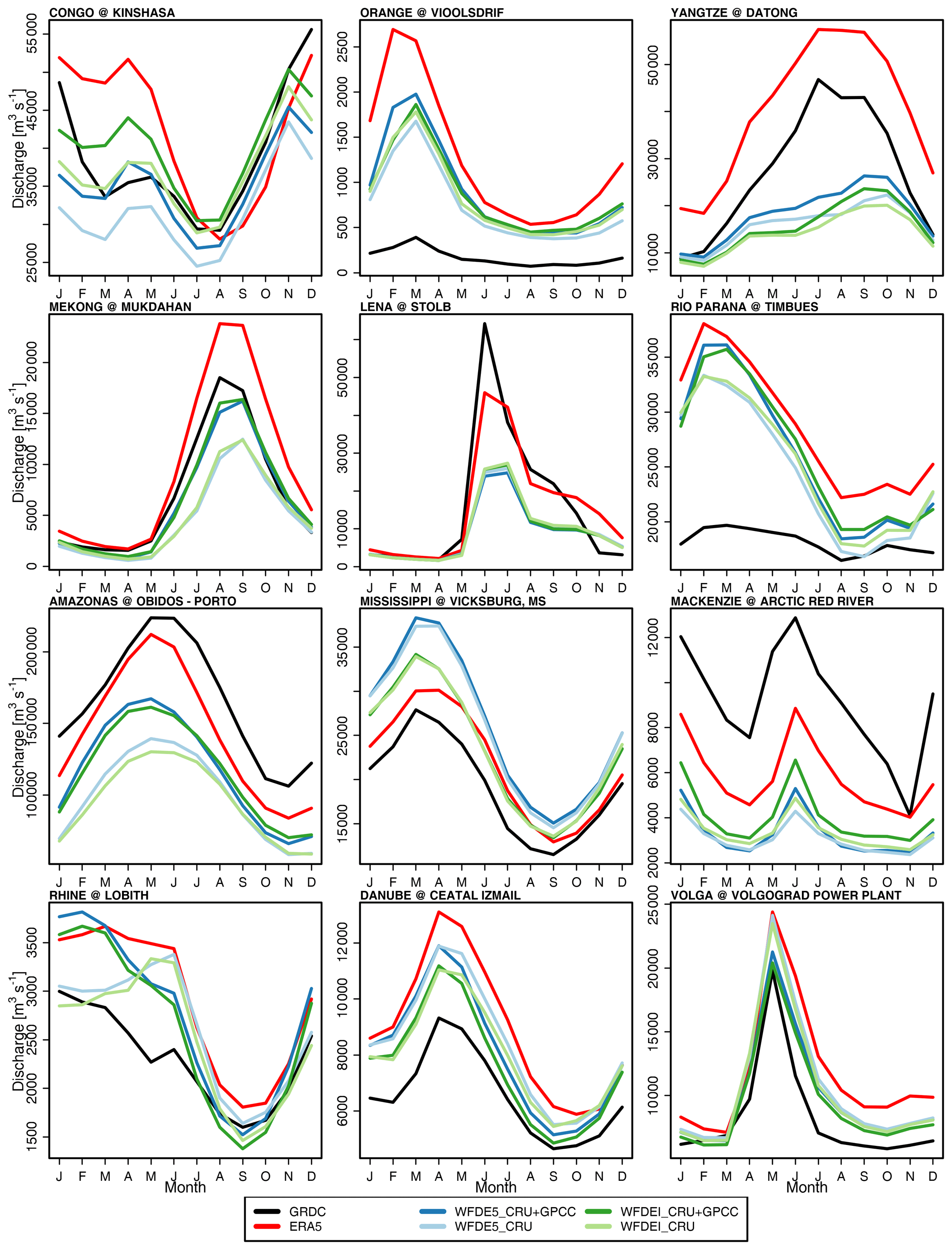
Figure 5 Seasonality of observed river discharge and uncalibrated WaterGAP runs for selected large river basins (Fig. 1).

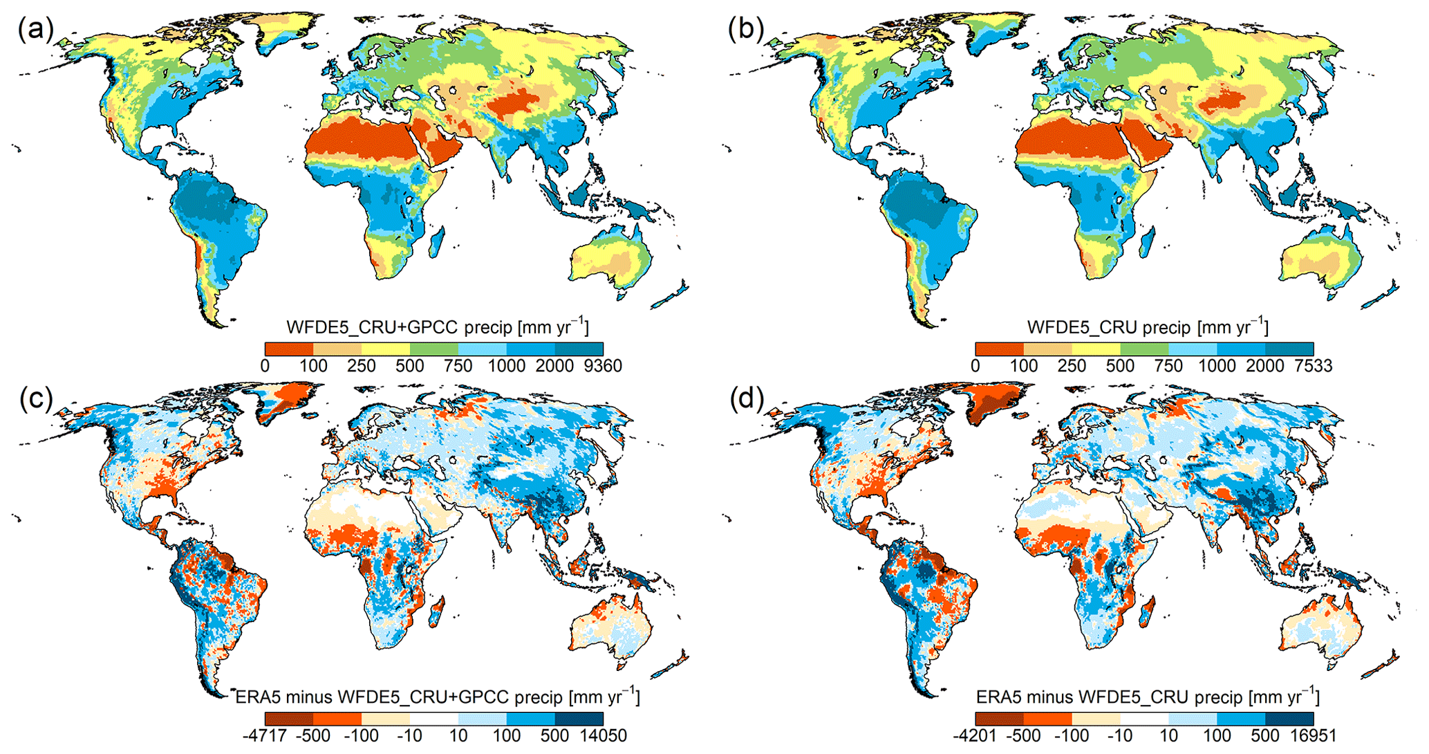
Figure 6 Long-term (1979–2016) average precipitation of the climate forcings, displayed as absolute number for WFDE5_CRU+GPCC (a), WFDE5_CRU (b), and differences to ERA5, computed as ERA5 minus WFDE5_CRU+GPCC (c) and ERA5 minus WFDE5_CRU (d). All values are given in millimetres per year.

In Fig. 5 discharge seasonality is shown with GRDC observations in black; see Fig. 1 for basin outlines. The figure shows the effect of adjusting precipitation from ERA5 (red in Fig. 5). For most basins, but not for all (e.g. Mississippi), the adjustment to CRU or GPCC-precipitation leads to a reduction of river discharge; this is substantial for some basins, e.g. Yangtze and Amazon. This does not necessarily lead to a better agreement with the observations (e.g. Amazon, Mackenzie, Lena), but for a number of basins it does (e.g. Congo, Orange, Mekong, Danube). Interestingly, the effect of the dataset chosen to adjust precipitation (CRU versus GPCC) is important for some basins (e.g. Mekong, Amazon). However, this is not relevant for other basins (e.g. Mississippi, Danube) where differences in WFDE5 and WFDEI compared to ERA5 and ERA-Interim for variables other than precipitation lead to different discharge simulations. An overview of spatial differences in long-term average precipitation between WFDE5 and ERA5 and can be found in Fig. 6 and help to interpret the patterns observed in Fig. 5. Spatial differences of the other variables used for WaterGAP are shown in Figs. A1–A3.

The validation with WaterGAP showed that using WFDE5 generally results in similar results to using WFDEI and should be preferred to using ERA5 directly. Nevertheless, this assessment was done using uncalibrated runs, thus a proper calibration to discharge observations could highlight the full benefit of WFDE5 compared to ERA5, but this is outside of the scope of this paper.

5 Application in ISIMIP

The WFDE5 dataset will be employed to drive historical impact simulations and bias-adjust future climate projections in the upcoming ISIMIP phase 3. The dataset is well suited for these purposes in particular thanks to its inter-variable consistency, which matters for the simulation of extreme climate impact events (Zscheischler et al., 2019). Thanks to a new bias adjustment method that is applied in ISIMIP phase 3, that is able to adjust inter-variable statistical dependencies (Lange, 2019b, 2020), the inter-variable consistency of WFDE5 will be beneficial for the bias adjustment of future climate projections as well.

Instead of using WFDE5 directly for these purposes, a derived dataset covering land and ocean with daily temporal resolution and including additional variables will be used in ISIMIP phase 3. This derived dataset consists of WFDE5 over land merged with ERA5 over the ocean (W5E5; Lange, 2019b). It covers land and ocean to facilitate impact studies everywhere and prevent mismatches between land–sea masks used by impact models. It has daily temporal resolution because that is sufficient to drive most impact models taking part in ISIMIP. Additional variables (2 m relative humidity, sea level pressure, total precipitation, daily maximum 2 m air temperature, daily minimum 2 m air temperature) derived from those included in WFDE5 are included in W5E5 to meet additional impact model requirements. More information about the W5E5 dataset is provided by Lange (2019b).

6 Code and data availability

The full information regarding access to the datasets can be found in Sect. 3.

7 Conclusions

The WFDE5 dataset will be useful for forcing surface models and especially for near-recent hydrological and agricultural analyses. It will also be used for bias correction of the CMIP6 GCM model output in the third phase of ISIMIP. WFDE5 benefits from the improvements of ERA5 compared to ERA-Interim, as well as from the additional corrections of temperature, precipitation, and shortwave radiation described above.

WFDE5 is provided at hourly time steps versus 3-hourly time steps for WFDEI. Comparison to observations from 13 FLUXNET2015 sites distributed globally shows that, on average, WFDE5 is superior to WFDEI for all variables in terms of mean absolute error and correlation. For precipitation and wind speed WFDE5 is superior to WFDEI at all 13 sites. Although both datasets are provided at 0.5^∘ resolution, WFDE5 has a greater spatial variability (Fig. 3) since it is obtained by aggregation of higher-resolution ERA5 data rather than by interpolation of lower-resolution ERA-Interim data used in WFDEI. Initial analysis using an uncalibrated hydrological model (WaterGAP) has demonstrated that the bias correction to CRU or GPCC precipitation totals results in lower discharge throughout the year bringing the global hydrological balance into better agreement with previous studies. The corrections result in improvements towards observations relative to the use of unaltered ERA5 forcing (e.g. in the Congo, Orange, and Danube basins).

Currently the WFDE5 dataset spans from the start of 1979 to the end of 2018 (end of 2016 for Rainf_WFDE5_CRU+GPCC, and Snowf_WFDE5_CRU+GPCC). However, the open source Python code within the Climate Change Service Toolbox will allow users to expand the coverage back to the start of 1950 and forwards through 2019 and later for themselves. The data have been created at 0.5^∘ resolution to match the CRU grid, but gridded observations of precipitation totals are already available from GPCC at 0.25^∘ and MSWEPv2 at 0.1^∘ (Beck et al., 2019b). The future availability of gridded observations of near-surface temperature, diurnal temperature range, cloud cover, aerosol loading, and numbers of wet days would allow creation of WFDE5 data at higher spatial resolution than the current dataset.

Appendix A

Table A1 Tair metrics for each FLUXNET2015 site: ERA5 versus FN2015 and WFDE5 versus FN2015 at hourly time steps.

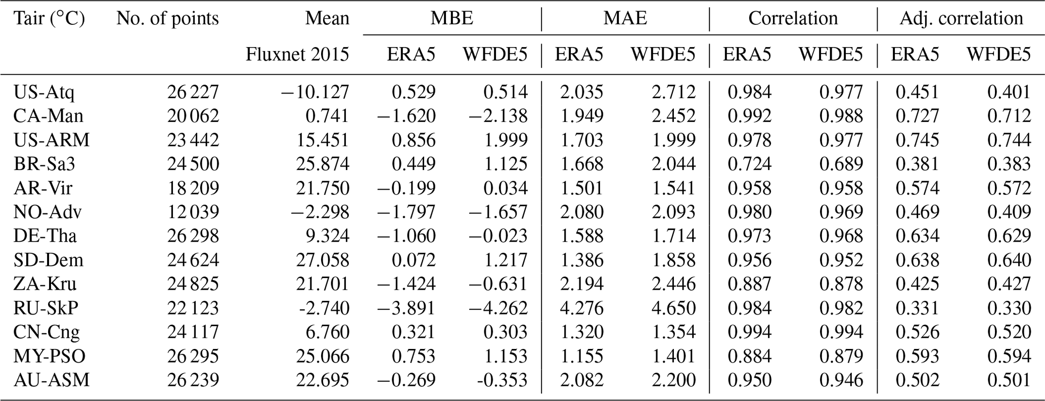
Table A2 PSurf metrics for each FLUXNET2015 site: ERA5 versus FN2015 and WFDE5 versus FN2015 at hourly time steps.

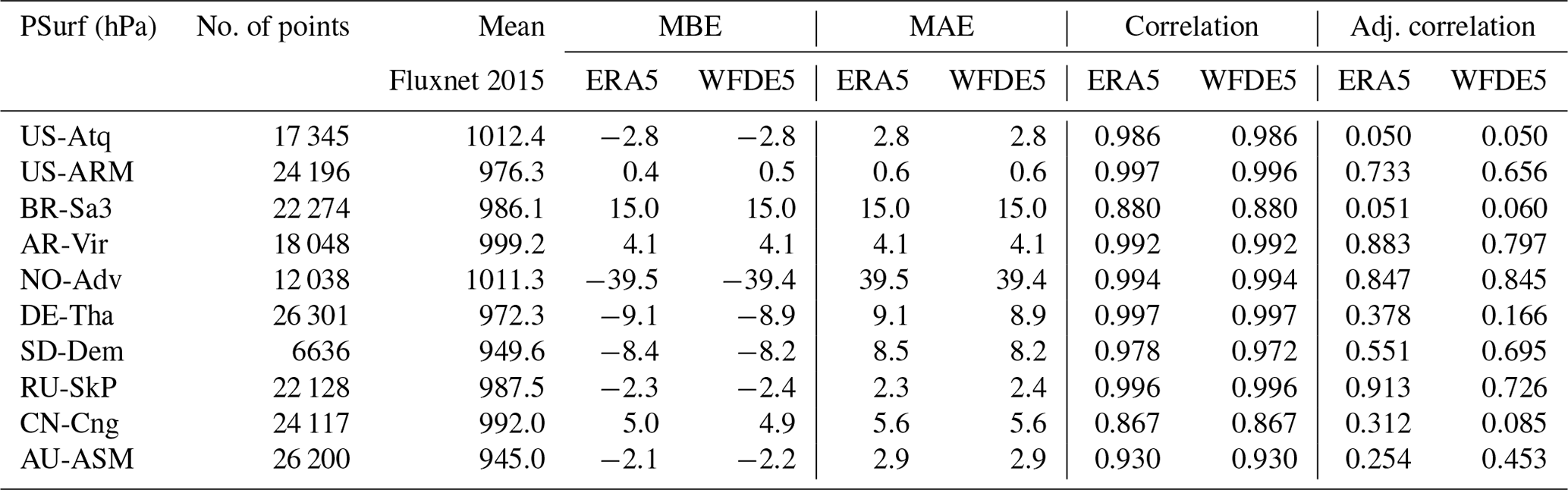
Table A3 Qair metrics for each FLUXNET2015 site: ERA5 versus FN2015 and WFDE5 versus FN2015 at hourly time steps.

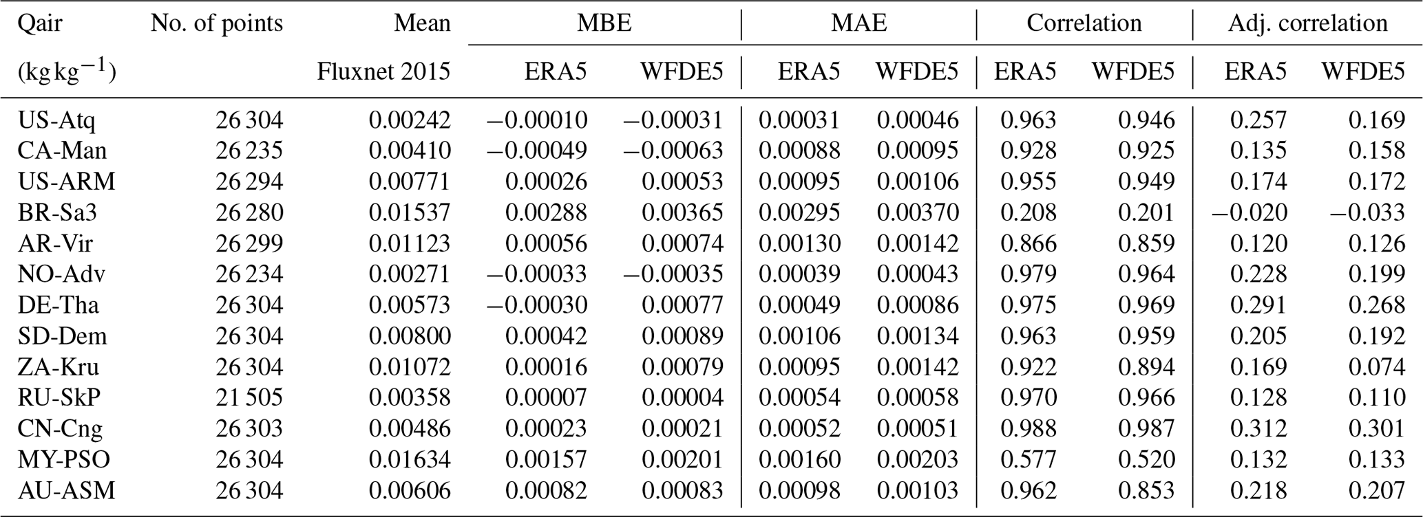
Table A4 Wind metrics for each FLUXNET2015 site: ERA5 versus FN2015 and WFDE5 versus FN2015 at hourly time steps.

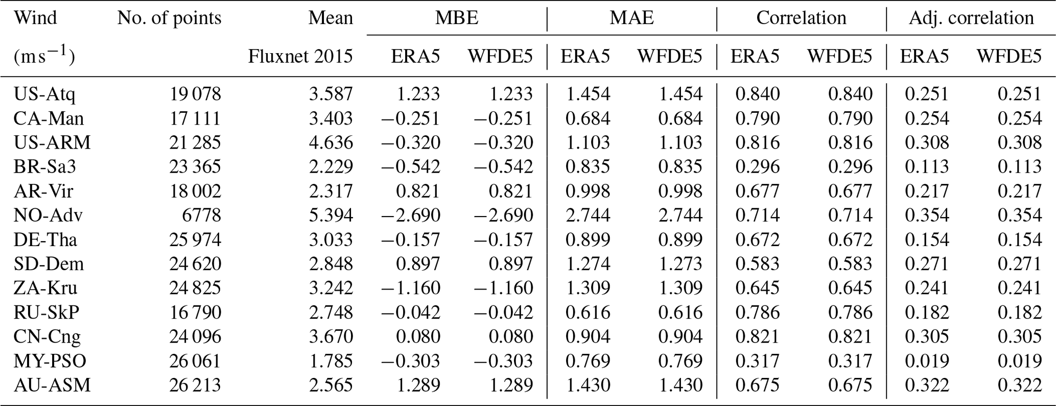
Table A5 SWdown metrics for each FLUXNET2015 site: ERA5 versus FN2015 and WFDE5 versus FN2015 at hourly time steps.

Table A6 LWdown metrics for each FLUXNET2015 site: ERA5 versus FN2015 and WFDE5 versus FN2015 at hourly time steps.

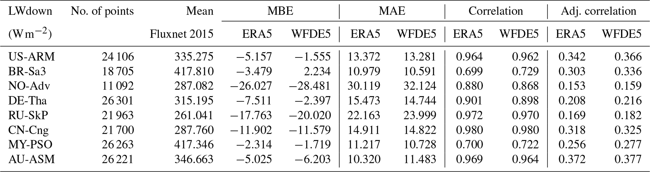
Table A7 Precipitation (Rainf + Snowf) metrics, corrected using CRU totals, for each FLUXNET2015 site: ERA5 versus FN2015 and WFDE5 versus FN2015 at hourly time steps.

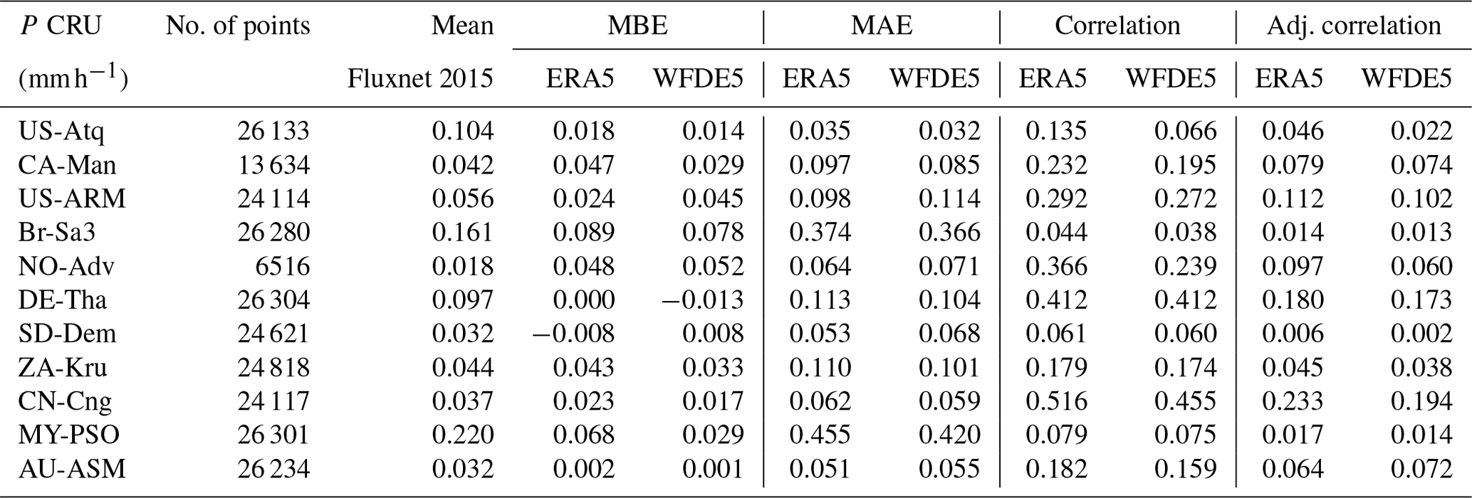
Table A8 Precipitation (Rainf + Snowf) metrics, corrected using GPCC totals, for each FLUXNET2015 site: ERA5 versus FN2015 and WFDE5 versus FN2015 at hourly time steps.

Table A9 Tair metrics for each FLUXNET2015 site: WFDEI versus FN2015 and WFDE5 versus FN2015 at 3-hourly time steps.

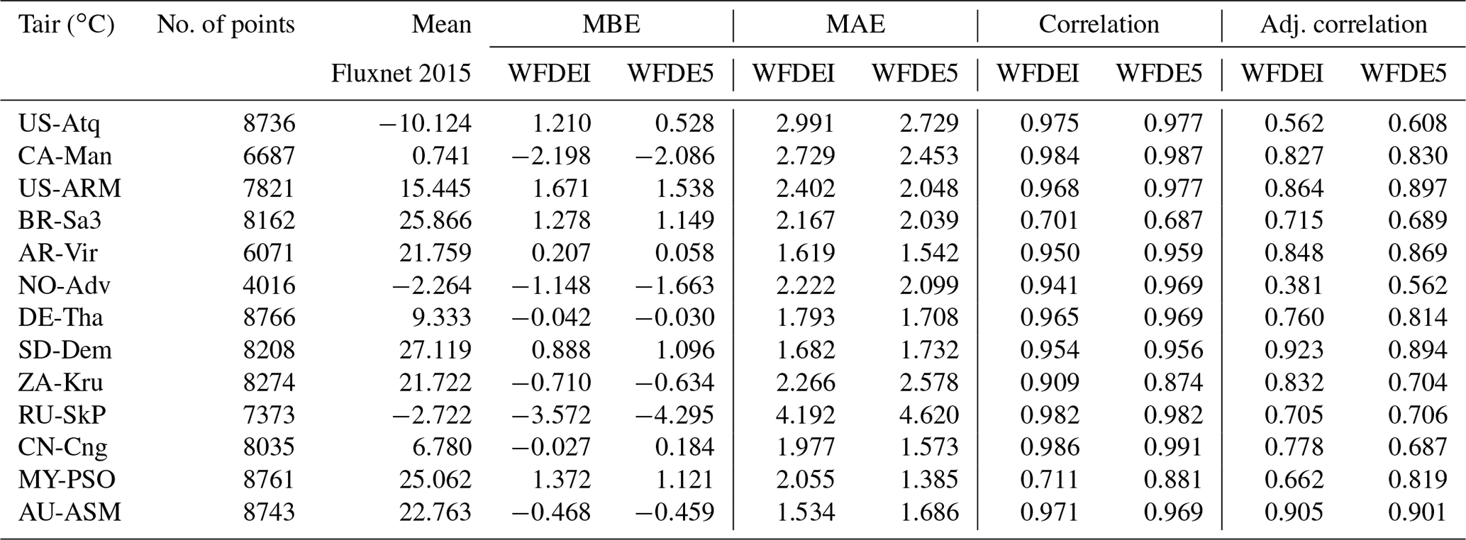
Table A10 PSurf metrics for each FLUXNET2015 site: WFDEI versus FN2015 and WFDE5 versus FN2015 at 3-hourly time steps.

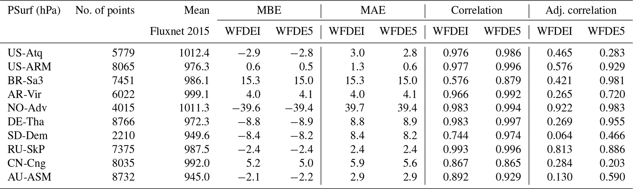
Table A11 Qair metrics for each FLUXNET2015 site: WFDEI versus FN2015 and WFDE5 versus FN2015 at 3-hourly time steps.

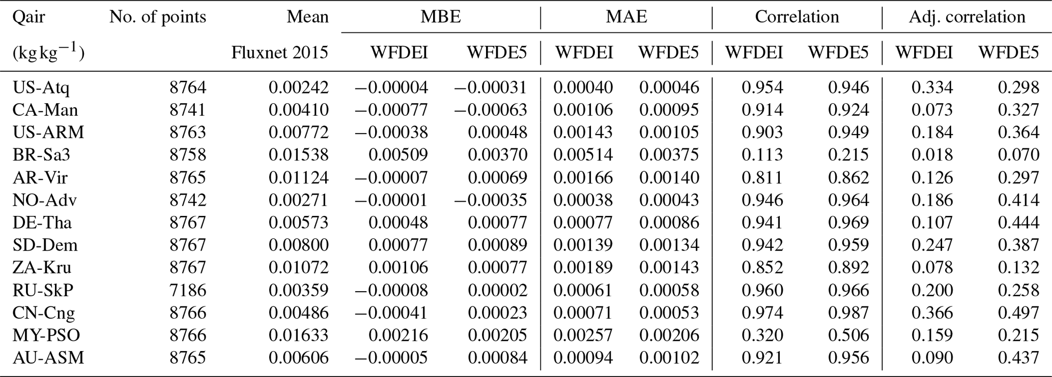
Table A12 Wind metrics for each FLUXNET2015 site: WFDEI versus FN2015 and WFDE5 versus FN2015 at 3-hourly time steps.

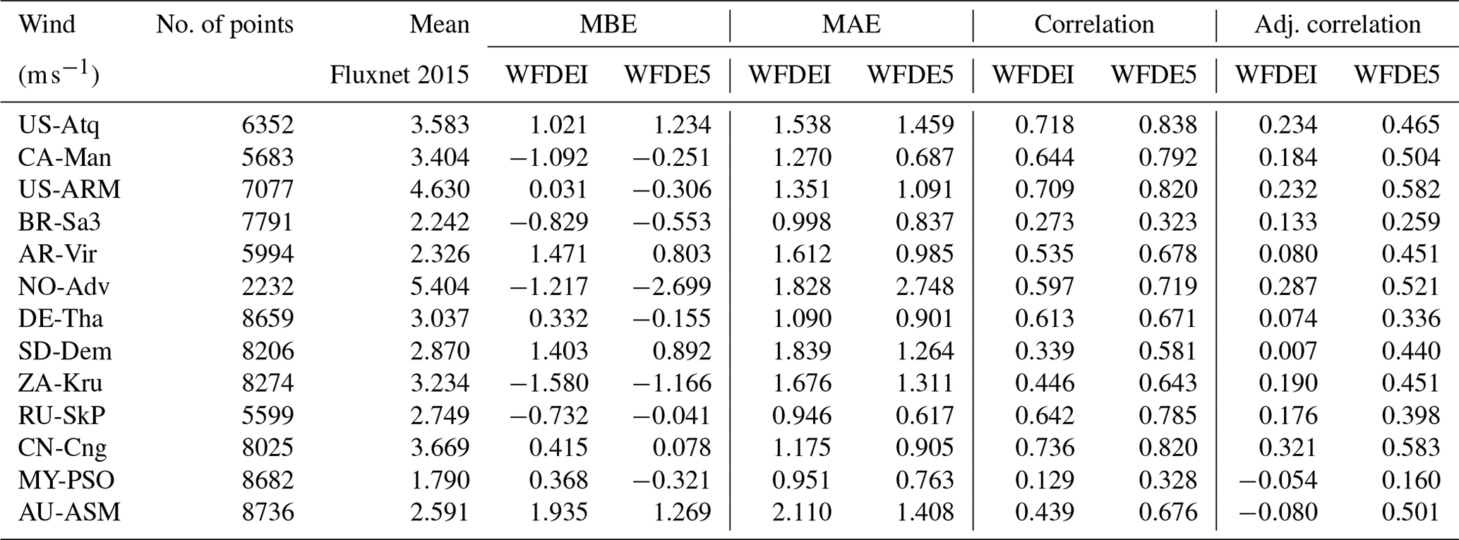
Table A13 SWdown metrics for each FLUXNET2015 site: WFDEI versus FN2015 and WFDE5 versus FN2015 at 3-hourly time steps.

Table A14 LWdown metrics for each FLUXNET2015 site: WFDEI versus FN2015 and WFDE5 versus FN2015 at 3-hourly time steps.

Table A15 Precipitation (Rainf + Snowf) metrics, corrected using CRU totals, for each FLUXNET2015 site: WFDEI versus FN2015 and WFDE5 versus FN2015 at 3-hourly time steps.

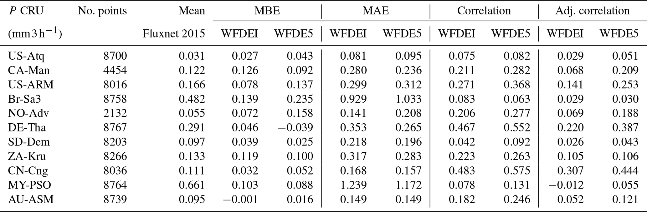
Table A16 Precipitation (Rainf + Snowf) metrics, corrected using GPCC totals, for each FLUXNET2015 site: WFDEI versus FN2015 and WFDE5 versus FN2015 at 3-hourly time steps.

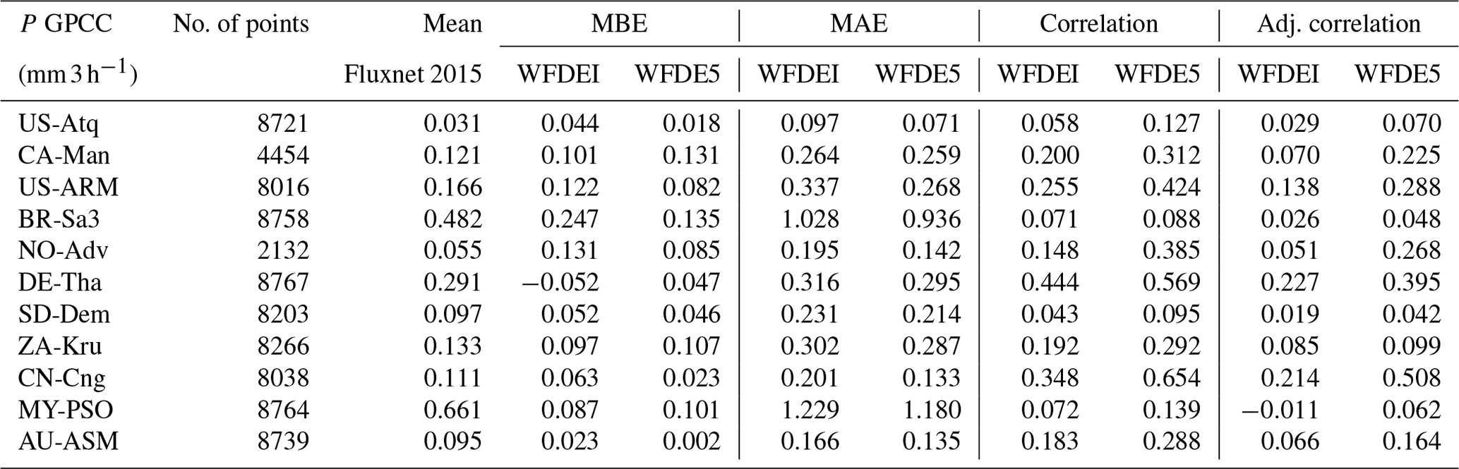
Table A17 Average metrics across all 13 FLUXNET2015 sites ±95 % confidence intervals of the means for ERA5 versus FN2015 and WFDE5 versus FN2015 at hourly time steps (see Tables A1–A8).

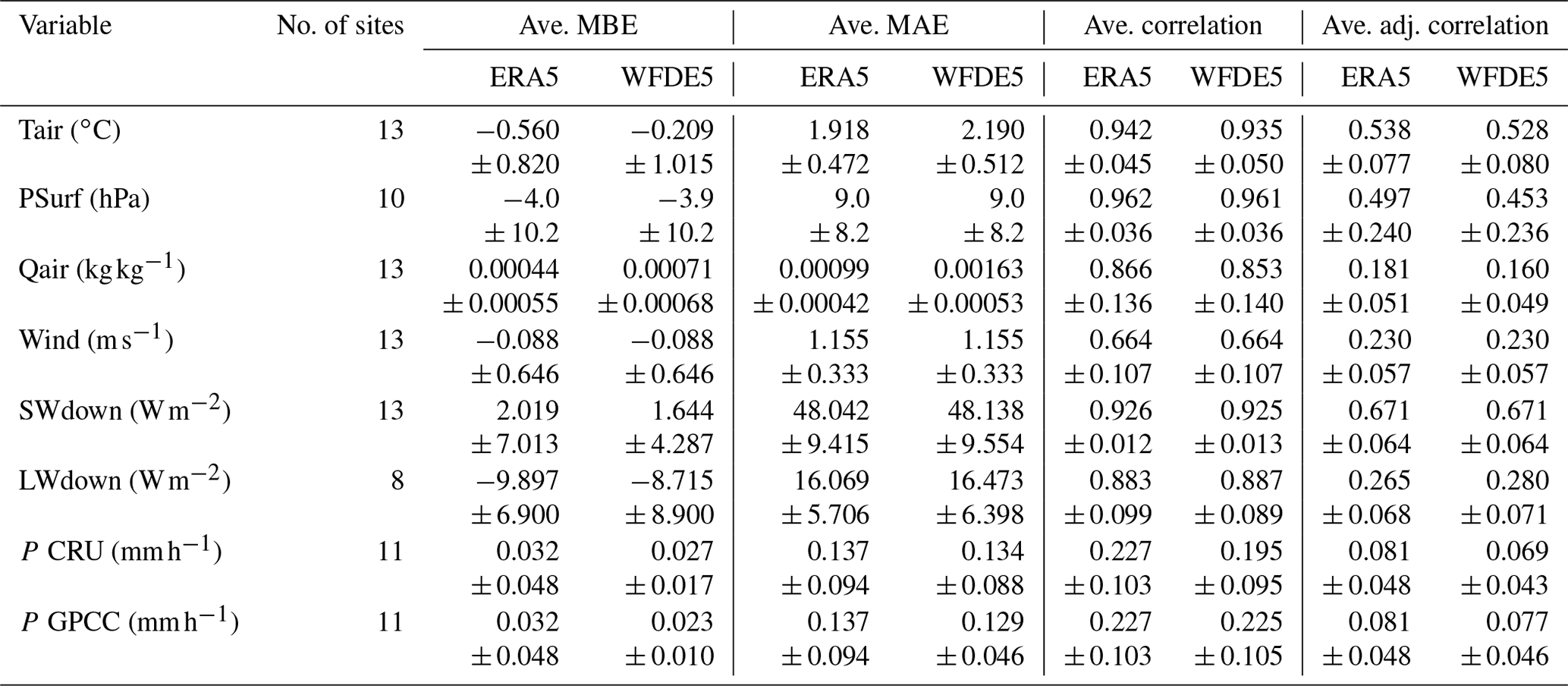
No. of sites stands for the number of sites with measurements for each variable. Ave. stands for average. Adj. stands for adjusted.

Table A18 Average metrics across all 13 FLUXNET2015 sites ±95 % confidence intervals of the means for WFDEI versus FN2015 and WFDE5 versus FN2015 at 3-hourly time steps (see Tables A9–A16)

No. of sites stands for the number of sites with measurements for each variable. Ave. stands for average. Adj. stands for adjusted.

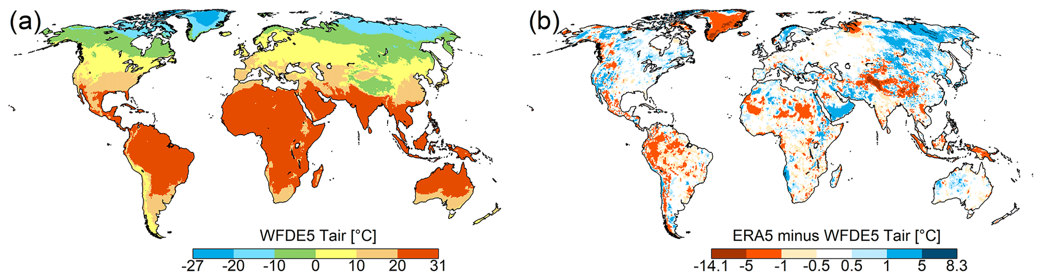
Figure A1 Long-term (1979–2016) average temperature of the climate forcings, displayed as absolute number for WFDE5 (a) and differences to ERA5, computed as ERA5 minus WFDE5 (b) (all values are given in ^∘C).

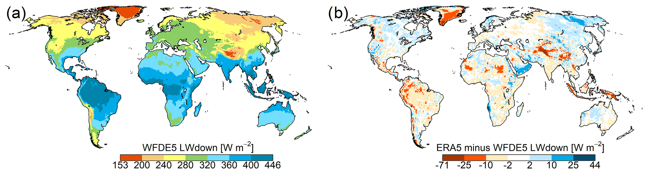
Figure A2 Long-term (1979–2016) average longwave downward radiation of the climate forcings, displayed as absolute number for WFDE5 (a) and differences to ERA5, computed as ERA5 minus WFDE5 (b) (all values are given in W m⁻²).

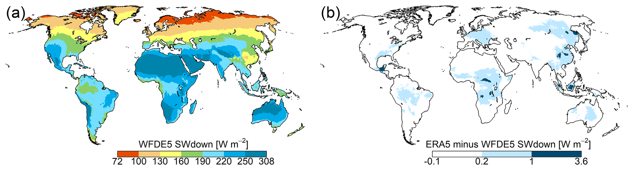
Figure A3 Long-term (1979–2016) average shortwave downward radiation of the climate forcings, displayed as absolute number for WFDE5 (a) and differences to ERA5, computed as ERA5 minus WFDE5 (b) (all values are given in W m⁻²).