Dissolved inorganic nutrients in the western Mediterranean Sea (2004–2017)

Long-term time series are a fundamental prerequisite to understanding and detecting climate shifts and trends. Understanding the complex interplay of changing ocean variables and the biological implication for marine ecosystems requires extensive data collection for monitoring, hypothesis testing, and validation of modelling products. In marginal seas, such as the Mediterranean Sea, there are still monitoring gaps, both in time and in space. To contribute to filling these gaps, an extensive dataset of dissolved inorganic nutrient observations (nitrate, phosphate, and silicate) was collected between 2004 and 2017 in the western Mediterranean Sea and subjected to rigorous quality control techniques to provide to the scientific community a publicly available, long-term, quality-controlled, internally consistent biogeochemical data product. The data product includes 870 stations of dissolved inorganic nutrients, including temperature and salinity, sampled during 24 cruises. Details of the quality control (primary and secondary quality control) applied are reported. The data are available in PANGAEA (https://doi.org/10.1594/PANGAEA.904172, Belgacem et al., 2019).

1 Introduction

Dissolved inorganic nutrients play a crucial role in marine ecosystem functioning. They serve as regulators of ocean biological productivity and are trace elements for biogeochemical cycling as well as for natural and anthropogenic sources and transport processes (Béthoux, 1989; Béthoux et al., 1992). They are also non-conservative tracers, since their distribution varies according to both biological (such as primary production and respiration) and physical (such as convection, advection, mixing, and diffusion) processes. Very schematically, inorganic nutrients are continuously consumed by phytoplankton (due to primary production) at the sea surface and regenerated in the mesopelagic layer by bacteria and animals (due to respiration). Moreover, the sinking of organic matter and its decomposition increase the nutrient concentrations in the intermediate- and deep-water masses over time. To identify the limiting factors for biological production in the oceans, we need to understand the underlying chemical constraints and especially the macro- and micronutrient spatial and temporal variations. Dissolved inorganic nutrients may be used as tracers of water masses like salinity and temperature to assess mixing processes and to understand the biogeochemical circumstances of their formation regions. Understanding the complex interplay of changing ocean variables and the biological implication for marine ecosystems is a difficult task and requires not only modelling but also extensive data collection for monitoring, hypothesis testing, and validation. Monitoring gaps still remain in both time and space, especially for marginal seas such as the Arctic Ocean or the Mediterranean Sea.

The Mediterranean Sea has been identified as a region significantly affected by ongoing climatic changes, like warming and a decrease in precipitation (Giorgi, 2006). In addition, it is a region particularly valuable for climate change research because it behaves like a miniature ocean (Béthoux et al., 1999) with a well-defined overturning circulation characterized by spatial and temporal scales that are much shorter than for the global ocean, with a turnover of only several decades. Being an intercontinental sea and subjected to more terrestrial nutrient inputs (river runoff, submarine groundwater discharge) and atmospheric deposition, the Mediterranean Sea has a nitrate to phosphate N:P ratio that is anomalously high compared to the “classical” world oceans Redfield ratio, indicating a general P-limitation regime, which becomes stronger along a west-to-east gradient. The Mediterranean Sea is therefore a potential model for studying global patterns that will be experienced in the next decades worldwide, not only regarding ocean circulation but also the marine biota (Lejeusne et al., 2010). Several environmental variables can act as stressors for marine ecosystems, by which climatically driven ecosystem disturbances are generated (Boyd, 2011). These changes affect, among other things, the distribution of biogeochemical elements (including inorganic nutrients) and the functioning of the biological pump and CO₂ regulation.

Within this context, the aim of this paper is to compile an extensive dataset of dissolved inorganic nutrient observations (nitrate, phosphate, and silicate) collected between 2004 and 2017 in the western Mediterranean Sea (WMED); to describe the quality control techniques; and to provide the scientific community with a publicly available, long-term, quality controlled, and internally consistent biogeochemical data product, contributing to previously published Mediterranean Sea datasets like MEDAR/MEDATLAS (time period 1908–1999; Fichaut et al., 2003) and the Mediterranean Sea – Eutrophication and Ocean Acidification aggregated datasets v2018 (time period 1911–2017) provided by EMODnet Chemistry (Giorgetti al., 2018) available at https://www.seadatanet.org/Products/Aggregated-datasets (last access: March 2020).

2 Dissolved inorganic nutrient data collection

2.1 The CNR dissolved inorganic nutrient data in the WMED

Long-term time series, such as the OceanSITES global time series (http://www.oceansites.org, last access: May 2019), are a fundamental prerequisite to understanding and detecting climate shifts and trends. However, biogeochemical time series are still limited to the northern part of the western Mediterranean Sea (MOOSE network; Coppola et al., 2019). Yet, inorganic nutrients in the Mediterranean Sea have received more attention in recent years, and various datasets have been compiled to understand their unique characteristics such as the one built by the PERSEUS project consortium (Policy-oriented marine environmental research in the southern European seas”, EU FP7 project, grant agreement (GA) no. 287600), which included 100 cruises collected during the project's lifetime, in addition to those from other projects like SESAME (EU FP7 project, GA no. GOCE-036949) and data products such as MEDAR/MEDATLAS. In addition to that, the data assembly system EMODnet Chemistry, a leading infrastructure, is supported by the pan-European Directorate-General for Maritime Affairs and Fisheries (DG MARE; Martín Míguez et al., 2019; Tintoré et al., 2019).

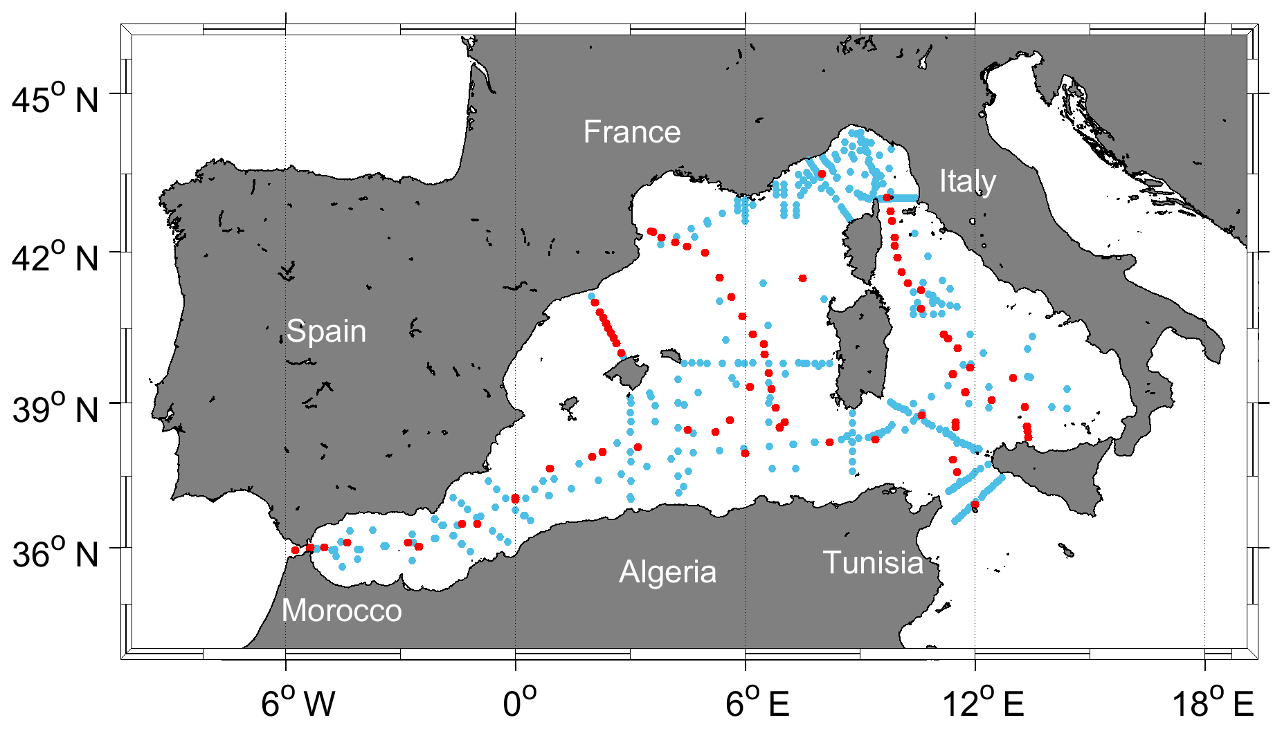
Figure 1 Map of the western Mediterranean Sea showing the biogeochemical stations (in blue) and the five reference cruise stations (in red).

Table 1 (a) Cruise summary table and parameters listed with number of stations and samples. Cruises were identified with an ID number and expedition code (EXPOCODE of format AABBYYYYMMDD – AA: country code; BB: ship code; YYYY: year; MM: month; DD: day indicative of cruise starting day). (b) Data sources and links to the reports (last access: June 2020).

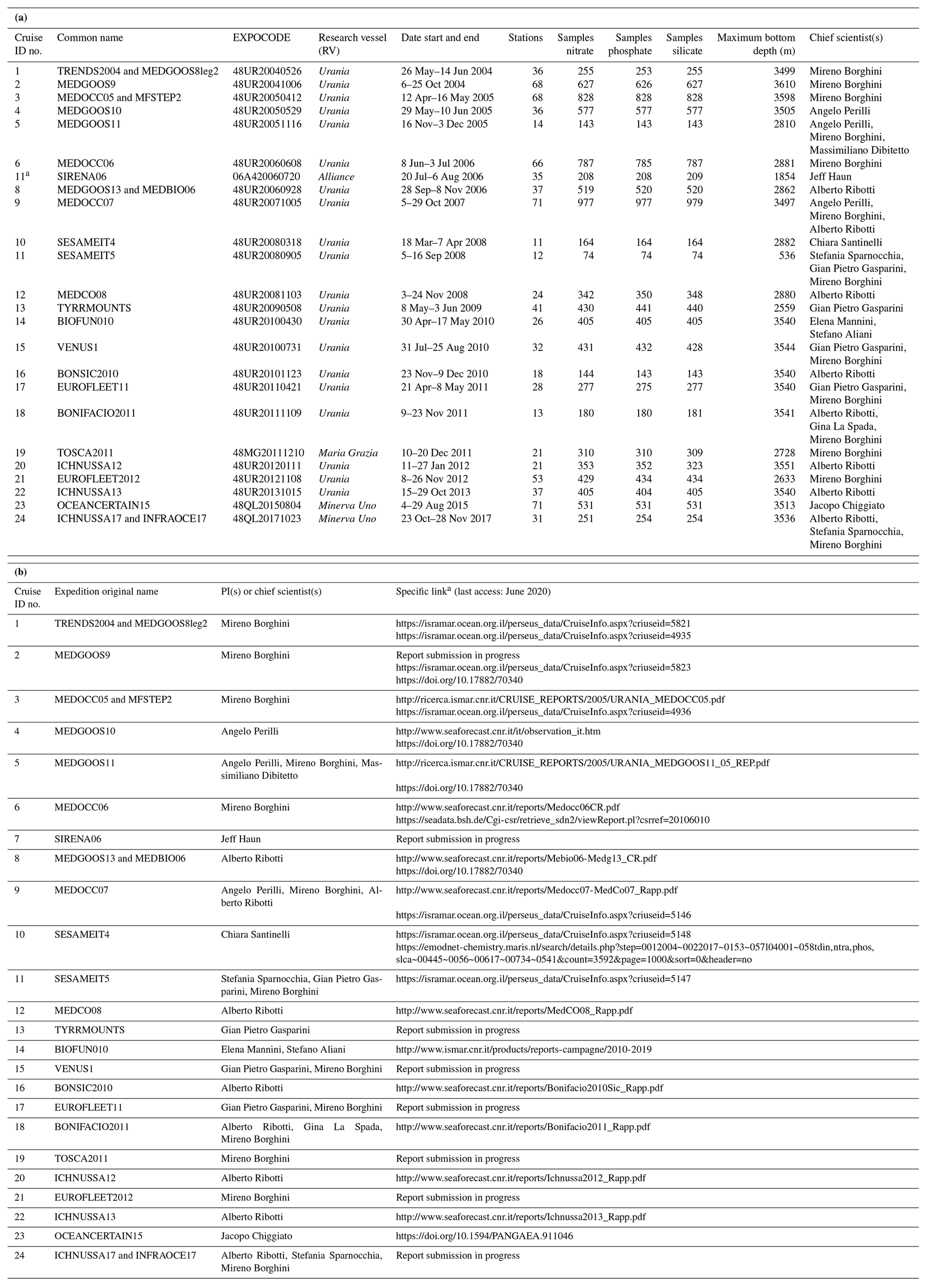
^a The specific links are subjectu7 to updates.

The dataset presented here consists of 24 oceanographic cruises (Fig. 1, Table 1a and b) conducted in the WMED on board research vessels run by the Italian National Research Council (CNR) and the NATO Science and Technology Organization (STO) Centre for Maritime Research and Experimentation (CMRE). All cruises were merged into a unified dataset with 870 nutrient stations and ∼9666 data points over a period of 13 years (2004–2017). The overall spatial distribution of the stations covers the whole WMED, but the actual distribution strongly varies depending on the specific cruise and most of the data are collected along sections. At all stations, pressure, salinity, and temperature were measured with a CTD-rosette system consisting of a CTD SBE 911plus and a General Oceanics rosette with 24 Niskin bottles of 12 L capacity. Temperature measurements were performed with the SBE 3F thermometer with a resolution of 10^−3 ∘C; conductivity measurements were performed with an SBE 4 sensor with a resolution of $\mathrm{3}\times {\mathrm{10}}^{-\mathrm{4}}$ S m⁻¹. The probes were calibrated before and after each cruise. During all CNR cruises, redundant sensors were used for both temperature and salinity measurements.

Seawater samples for dissolved inorganic nutrient measurements were collected during the CTD upcast at standard depths (with slight modifications according to the depth at which the deep chlorophyll maximum was detected). The standard depths are usually 5, 25, 50, 75, 100, 200, 300, 400, 500, 750, 1000, 1250, 1500, 1750, 2000, 2250, 2500, 2750, and 3000 m. No filtration was employed; nutrient samples were immediately stored at −20 ^∘C. Note that sample storage and freezing duration varied greatly from one cruise to another (Table 3 shows cruises where this exceeded 1 year).

2.2 Analytical methods for inorganic nutrients

For all cruises, nutrient determination (nitrate, orthosilicate, and orthophosphate) was carried out following standard colorimetric methods of seawater analysis, defined by Grasshoff et al. (1999) and Hansen and Koroleff (1999). For inorganic phosphate, the method is based on the reaction of the ions with an acidified molybdate reagent to yield a phosphomolybdate heteropoly acid, which is then reduced to a blue-coloured compound (absorbance measured at 880 nm). Inorganic nitrate is reduced (with cadmium granules) to nitrite that reacts with an aromatic amine, leading to the final formation of the azo dye (measured at 550 nm). Then, the nitrite that is separately determined must be subtracted from the total amount measured to get the nitrate concentration only. The determination of dissolved silicon is based on the formation of a yellow silicomolybdic acid reduced with ascorbic acid to a blue-coloured complex (measured at 820 nm).

Nutrient analysis was performed in three laboratories. From 2004 to 2013, all cruises nutrients were analysed by ENEA, while for those of 2015 (cruise no. 23) and 2017 (cruise no. 24), nutrient concentrations were analysed by ISMAR-CNR (ISMAR is the Institute of Marine Sciences). Referring to Table S1 in the Supplement, four different models of autoanalyser were used. Measurements from the autoanalyser were reported in micromoles per litre. Inorganic nutrient concentrations were converted to the standard unit of micromoles per kilogram, using sample salinity from CTD and a mean laboratory analytical temperature of 20 ^∘C. Data from nutrient analysis were then merged with ancillary CTD bottle data.

Table 2 Cruise summary table of the reference cruise collection used in the secondary quality control, collected from 2001 to 2016.

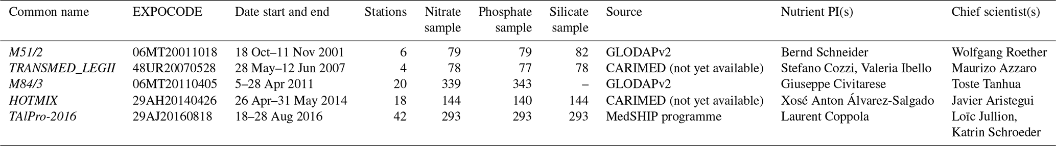
Figure 2 Overview of the reference cruise spatial coverage and vertical distributions of the inorganic nutrients. (a) Geographical distribution map; (b) vertical profiles of nitrate (µmol kg⁻¹); (c) vertical profiles of phosphate (µmol kg⁻¹); (d) vertical profiles of silicate (µmol kg⁻¹).

2.3 Reference inorganic nutrient data

In addition to the data collected during the above-mentioned cruises and in order to perform the secondary quality control (described below), we identified five reference cruises (Table 2), based on their spatial and temporal distribution and the reliability of the measurements (see Fig. 2 and Table S3 and Fig. S1 in the Supplement). Cruises 06MT20110405 and 06MT20011018 are the only two Mediterranean cruises included in the publicly available Global Ocean Data Analysis Project version 2 (GLODAPv2; Olsen et al., 2016). These cruises, conducted on board the R/V Meteor, provide a reliable reference because nutrient analysis strictly followed the recommendation of the World Ocean Circulation Experiment (WOCE) and the GO-SHIP protocols (Hydes et al., 2010; Tanhua et al., 2013). Cruises 29AH20140426 and 48UR20070528 are to be included in the CARIMED data product (personal communication by Marta Álvarez, in preparation but not yet available) and have undergone rigorous quality control following GLODAP routines. Finally, 29AJ20160818 was carried out in the framework of the MedSHIP programme (Schroeder et al., 2015), and its data are available at https://doi.org/10.1594/PANGAEA.902293 (Tanhua, 2019).

3 Quality assurance and quality control methods

Combining inorganic nutrient data from different sources, collected by different operators, stored for different amounts of time, and analysed by multiple laboratories is not a straightforward task. This is widely recognized in the biogeochemical oceanographic community. Since the 1990s, several studies and programmes (e.g. World Ocean Database, World Ocean Atlas, WOCE) have been devoted to facilitating the exchange of oceanographic data and developing quality control procedures to compile databases by the estimation of systematic errors (Gouretski and Jancke, 2000) to increase inter-comparability, generate consistent datasets, and accurately observe long-term change.

An example of a first quality control procedure is the use of reference materials that are available for salinity (IAPSO – International Association for Physical Sciences of the Ocean, salinity standard by OSIL – Ocean Scientific International Limited) and temperature (SPRT – standard platinum resistance thermometer). As for the inorganic carbon, total alkalinity (Dickson et al., 2003), and inorganic nutrients (Aoyama et al., 2016), certified reference materials (CRMs) have been recently made applicable for oceanographic cruises. However, since CRMs are not always available or used for biogeochemical oceanographic data, Lauvset and Tanhua (2015) developed a secondary quality control tool to identify biases in deep data. The method suggests adjustments that reduce cruise-to-cruise biases, increase accuracy, and allow for the inter-comparison between data from various sources. This approach, based on a crossover and inversion method (Gouretski and Jancke, 2000; Johnson et al., 2001), was used to generate the CARbon dioxide IN the Atlantic Ocean (CARINA; see Hoppema et al., 2009), GLODAPv2.2019 (Olsen et al., 2019), and PACIFICA (Suzuki et al., 2013) data products.

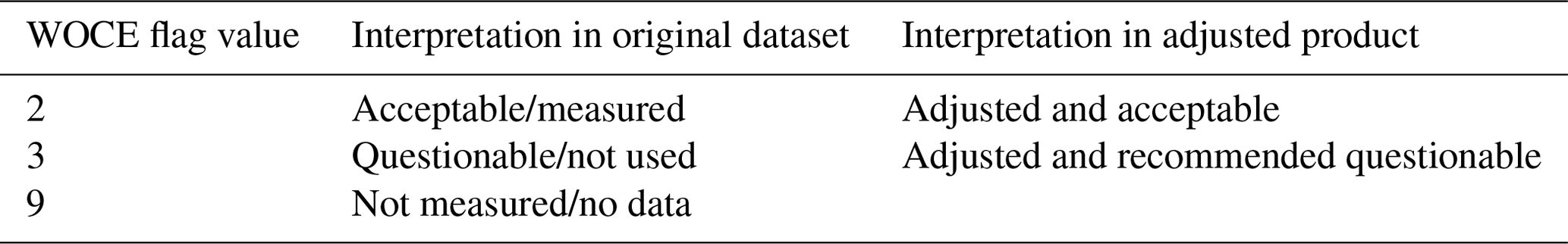
Table 3 WOCE flags used in the original data product and in the adjusted product.

3.1 Primary quality control

Each individual cruise was first subjected to a primary quality control (first QC) that included a check of apparent and extreme outliers in CTD salinity, nitrate, phosphate, and silicate. Each parameter included a quality control flag, following standard WOCE flags (Table 3). The surface, intermediate, and deep layer were evaluated separately because nutrient observations evolve differently in each layer. The coefficient of variation (CV, defined as standard deviation over mean) was computed for each depth layer. Coefficients of variation in the surface layer (0–250 db) were high (nitrate CV=1.16, phosphate CV=1.005, silicate CV=0.75) due to air–sea interaction (Muniz et al., 2001) occurring in this layer rendering it difficult to flag. These influences are of reduced importance in the intermediate layer (250–1000 db; nitrate CV=0.23, phosphate CV=0.31, silicate CV=0.24) and the deep layer (>1000 db; nitrate CV=0.15, phosphate CV=0.22, silicate CV=0.14), decreasing the total variance. Flags in the upper and intermediate layer were thus set based on outliers within pressure ranges defined according to standard pressures (0–10, 10–30, 30–60, 60–80, 80–160, 160–260, 260–360, 360–460, 460–560, 560–1000 db).

Below 1000 db, flagging included an inspection of nitrate to phosphate (N:P) and nitrate to silicate (N:Si) ratios. The median and median absolute deviation (MAD) were computed by classes of pressure: we considered outliers to be any atypical observation and any value that departs from the median by more than three MADs in the different pressure ranges for each cruise.

Figure 3 Scatter plots of (a) phosphate vs. nitrate (µmol kg⁻¹) and (b) silicate vs. nitrate (µmol kg⁻¹). Data that have been flagged as questionable (flag 3) are in red; the colour bar indicates the pressure (dbar). The black lines represent the best linear fit between the two parameters, and the corresponding equations and r² values are shown in each plot. Average resulting N:P ratio is 20.87; average resulting N:Si ratio is 1.05 (whole depth).

An overview of the nutrient distribution is provided with scatter plots, showing also the flagged measurements (Fig. 3). Each measurement was flagged as 2 (“Acceptable/measured”) or flagged as 3 (“Questionable”); 4.1 % of nitrate data, 3.37 % of phosphate data, 3.16 % of silicate data, and 0.07 % of CTD salinity data were considered outliers and flagged as 3. As highlighted by Tanhua et al. (2010), the primary QC can be subjective depending on the expertise of the person flagging the data, thus flagging could bring in some uncertainties.

Table 4 Average and standard deviations of nitrate, phosphate, and silicate measurements by cruise and for each region with number of samples deeper than 1000 db included in the second QC. Average storage time is the minimum storage time defined as time difference between the cruise ending day and the first day of the laboratory analysis.

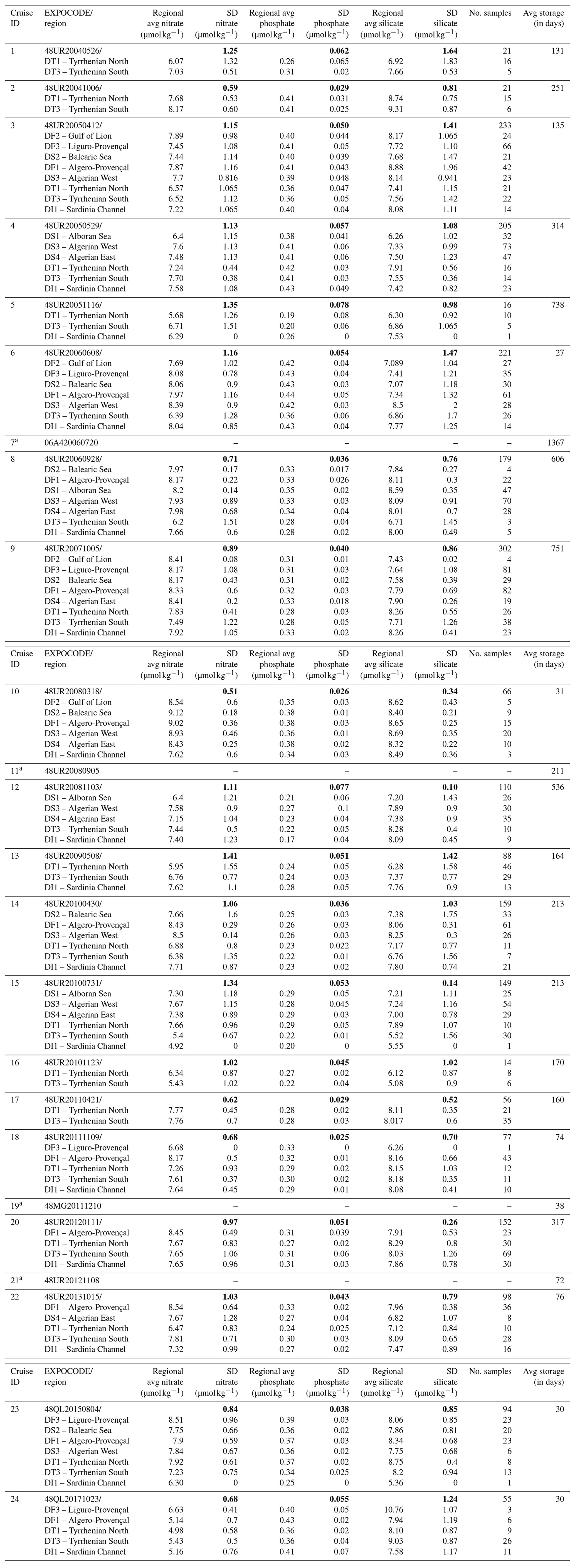
^a Cruise not included in the second QC (Sect. 4). In bold: the overall standard deviation by cruise; in normal font: regional standard deviation by cruise.

In order to have a first assessment of the precision of each cruise set of measurements, the standard deviation of observations deeper than 1000 db was calculated along with averages and standard deviations for each cruise and by subregion to have an overview of nutrient content variability in the deep layer and of the observations' spatial spread of individual cruises (Table 4). Following the subdivision of Manca et al. (2004), the WMED has been divided into subregions (Fig. S2, Table S2) according to the general circulation patterns (details in Manca et al., 2004). Table 4 displays the comparison of standard deviation of deep measurements for each cruise and within subregions. The overall standard deviation between cruises in the deep layer varied between 0.51 and 1.41 µmol kg⁻¹ for nitrate, between 0.1 and 1.64 µmol kg⁻¹ for silicate, and between 0.025 and 0.078 µmol kg⁻¹ for phosphate. Regional standard deviation of nitrate measurements below 1000 db varied between 0.08 µmol kg⁻¹ in the Gulf of Lion (DF2) with cruise no. 9 and 1.6 µmol kg⁻¹ in the Balearic Sea (DS2) observations of cruise no. 14. The lowest phosphate regional standard deviation was 0.01 µmol kg⁻¹ found in the observations of cruise no. 9 in the Gulf of Lion (DF2), cruise no. 10 in the Balearic Sea (DS2) and Algerian West (DS3), cruise no. 14 and cruise no. 15 in the Tyrrhenian South (DT3), and cruise no. 18 in Algero-Provençal (DF1) and the Sardinia Channel (DI1), while the highest standard deviation was 0.1 µmol kg⁻¹ in the observations of cruise no. 12 in the Algerian West (DS3). As for silicate, the lowest standard deviation was 0.02 µmol kg⁻¹ observed in cruise no. 9 measurements of the Gulf of Lion subregion (DF2) and the highest deep standard deviation was observed in cruise no. 6 in all its subregions together with cruise no. 5 measurements in the Tyrrhenian North (DT1) with a 1.83 µmol kg⁻¹ standard deviation.

Cruises no. 3, no. 6, and no. 9 had the largest spatial extension (see right side of Fig. 9) with a high number of samples over more than seven subregions (Table 4); the geographical variability in the distribution of dissolved inorganic nutrients results thus in the largest standard deviations. Conversely, cruises with smaller spatial coverages have lower standard deviations. Therefore, a relatively small spatial coverage and high standard deviation is considered as indicative of data with low precision (Olsen et al., 2016). This applies to cruises no. 1, no. 5, and no. 16. Despite the small spatial coverage, samples of nitrate and phosphate of cruise no. 5 have an overall standard deviation of 1.35 and 0.07 µmol kg⁻¹, respectively, a high standard deviation was also pointed out in the regional standard deviation of deep measurements in the Tyrrhenian North (DT1) and South (DT3). Cruise no. 1, with few stations in the Tyrrhenian North (DT1) and South (DT3) subregions and 21 samples below 1000 db, has an overall standard deviation of 1.25 µmol kg⁻¹ for nitrate, 0.06 µmol kg⁻¹ for phosphate, and 1.64 µmol kg⁻¹ for silicate. The regional standard deviation was relatively high for nitrate (0.51–1.32 µmol kg⁻¹), phosphate (0.02–0.065 µmol kg⁻¹), and silicate (0.53–1.83 µmol kg⁻¹). A comparison with the deviations from e.g. cruise no. 2, carried out in the same year and e.g. cruise no. 17 (with a similar cruise track) confirms the lower precision of the data of cruise no. 1. Similar considerations apply to the quality of nitrate samples (0.87–1.02 µmol kg⁻¹) and silicate (0.87–0.9 µmol kg⁻¹) from cruise no. 16, covering a small area in the Tyrrhenian North (DT1) and South (DT3), compared to cruise no. 17, carried out in the same regions (right side of Fig. 9 and Table 4).

Deep silicate measurements of cruise no. 6 have twice the overall standard deviation of silicate data of cruise no. 8 from the same year. Adding to that, in the seven subregions, the regional standard deviation of deep silicate observations was the highest, between 1.04 and 2 µmol kg⁻¹, which was relatively high compared to the surrounding cruises that have observations in the same subregions. This is again suggestive of limited precision. On the other hand, trying to explain the source of relatively high standard deviations in specific cruises is not always straightforward, as they could stem from a variety of sources, sampling, and conservation and analysis methods. The bottom water in the WMED exhibits a high nutrient content below 1000 db (Table 4), due to the longer residence time. Dividing the WMED into subregions has effectively removed the natural spatial change in nutrients, making the interpretation of the standard deviation a matter of the precision of the measurements only.

In Table 4, deep averages by subregions show that overall nutrient concentration fluctuated at around 7.4±0.9 µmol kg⁻¹ for nitrate, 0.3±0.06 µmol kg⁻¹ for phosphate, and 7.7±0.8 µmol kg⁻¹ for silicate; similar findings were reported by Manca et al. (2004). Comparing cruise averages in each region enabled the identification of “suspect” cruises. Cruise no. 24 has the lowest deep average in nitrate in the Algero-Provençal (DF1) and Tyrrhenian North (DT1) subregions and in the Sardinia Channel (DI1). Silicate of cruises no. 24 and no. 16 was very low compared to the overall regional average in the Liguro-Provençal (DF3) and Tyrrhenian South (DT3) subregions. The deep average of phosphate did not show any outlier cruises in all subregions. Different reasons could explain the low precision in the samples; freezing is one. Although it is a valid preservation method (Dore at al., 1996), the error is higher when samples are not analysed immediately (Segura-Noguera et al., 2011), so the storage time could be influential.

3.2 Secondary quality control – the crossover analysis

The method used to perform the secondary QC on the WMED dissolved inorganic nutrient dataset makes use of the quality-controlled reference data and the crossover analysis toolbox developed by Tanhua (2010) and Lauvset and Tanhua (2015). The computational approach is based on comparing the cruise dataset to a high-quality reference dataset to quantify biases, described in detail in Tanhua et al. (2010). Here, we summarize the technique with emphasis on inorganic nutrients. The first step consisted of selecting reference data, as described in Sect. 2.3. The second step is the crossover analysis that was carried out using a MATLAB toolbox (available online at https://cdiac.ess-dive.lbl.gov/ftp/oceans/2nd_QC_Tool_V2/, last access: April 2018) where crossovers are generated as the difference between two cruises using the “running cluster” crossover routine. Each cruise is thus compared to the chosen set of reference cruises. For each crossover, samples deeper than 1000 db are selected within a predefined maximum distance set to a 2 arcdeg distance, defined as a crossing region, to ensure the quality of the offset with a minimum number of crossovers and to minimize the effect of the spatial change. The reason to select measurements deeper than 1000 db is to remove the high frequency variability associated with mesoscale features, biological activity, and the atmospheric forcing acting in the upper layers that might induce changes in the biogeochemical properties of water masses. On the other hand, the deep Mediterranean also cannot be considered truly unaffected by changes, as it is intermittently subjected to ventilation (Schroeder et al., 2016; Testor et al., 2018) and the real variability can be altered in adjusting data. The computational approach takes this into account, since weights are given to the less variant profile in the crossing region, according to the confidence in the determined offset of the compared profiles (i.e. the weighted mean offset of a given crossover pair is weighted to the depth where the offsets of all compared profiles have the smallest variation, which indeed is strongly interlinked with the degree of variance of each profile; for further details see Lauvset and Tanhua, 2015).

Before identifying crossovers, each profile was interpolated using the piecewise cubic Hermite method and the distance criteria outlined in Lauvset and Tanhua (2015) in their Table 1a, detailed in Key et al. (2004). The crossover is a comparison between each interpolated profile of the cruise being evaluated and the interpolated profile of the reference cruise. The result is a weighted offset (defined as the ratio between cruise and reference) and a standard deviation of the offset. The standard deviation is indicative of the precision – however, it is important to note that this assumption only works because it is a comparison to a reference – and the absolute offset is indicative of accuracy.

The third step consists of evaluating and selecting the suggested correction factor that was applied to the whole water column. The correction factor was calculated from the weighted mean offset of all crossovers found between the cruise and the reference dataset, involving a somewhat subjective process.

For inorganic nutrients, offsets are multiplicative so that a weighted mean offset >1 means that the measurements of the corresponding cruise are higher than the measurements of the reference cruise in the crossing region and applying the adjustment would decrease the measured values. The magnitude of an increase or a decrease is the difference in the weighted offset from 1. In general, no adjustment smaller than 2 % (accuracy limit for nutrient measurements) is applied (detailed description is found in Hoppema et al., 2009; Lauvset and Tanhua, 2015; Olsen et al., 2016; Sabine et al., 2010; Tanhua et al., 2010).

The last step is the computation of the weighted mean (WM) to determine the internal consistency and quantify the overall accuracy of the adjusted product (Hoppema et al., 2009; Sabine et al., 2010; Tanhua et al., 2009), with the difference that our assessment is based on the offsets with respect to a set of reference cruises. This WM reflects the absolute weighted mean offset of the dataset compared to the reference dataset; hence the smaller the WM, the higher the internal consistency. The accuracy was computed from the individual absolute weighted offsets. The WM, which will be discussed in Sect. 4.4, was computed using the individual weighted absolute offset (D) of the number of crossovers (L) and the standard deviation (σ): $\text{WM}=\frac{\sum _{i=\mathrm{1}}^{L}D\left(i\right)/(\mathit{\sigma }\left(i\right){)}^{\mathrm{2}}}{{\sum }_{i=\mathrm{1}}^L\mathrm{1}/(\mathit{\sigma }\left(i\right){)}^{\mathrm{2}}}$.

4 Results of the secondary QC and recommendations

The results of the secondary QC revealed the necessary corrections for nitrate, phosphate, and silicate. Four cruises were not considered in the crossover analysis: cruises no. 7 and no. 11 do not have enough stations >1000 db (at least three are needed to obtain valid statistics), while cruises no. 19 and no. 21 were outside the spatial coverage of the reference cruises. Cruises that were not used for the crossover analysis are made available in the original dataset but were not included in the final data product (see Supplement – Part 2, A2).

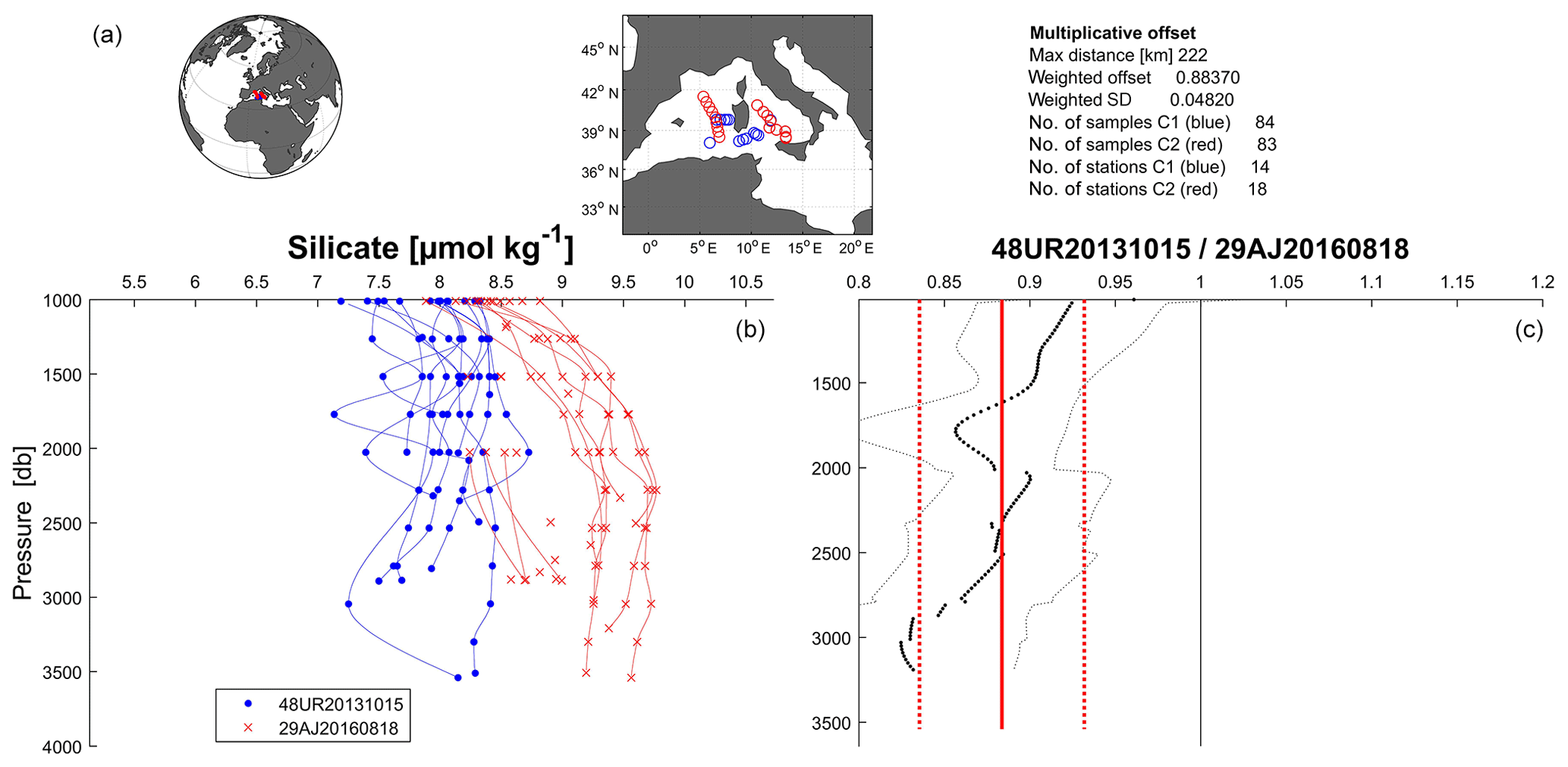
Figure 4 An example of the calculated offset for silicate between cruise 48UR20131015 and cruise 29AJ2016818 (reference cruise). (a) Location of the stations that are part of the crossover and statistics. (b) Vertical profiles of silicate data (µmol kg⁻¹) of the two cruises that fall within the minimum distance criteria (the crossing region), below 1000 dbar. (c) Vertical plot of the difference between both cruises (thick dotted black line) with standard deviations (thin dotted black lines) and the weighted average of the offset (solid red line) with the weighted standard deviations (dotted red lines).

Table 5 Summary of the suggested adjustment for nitrate, phosphate, and silicate resulting from the crossover analysis. Adjustments for inorganic nutrient are multiplicative. NA denotes not adjusted, i.e. data of cruises that could not be used in the crossover analysis, because of the lack of stations or because data are outside the spatial coverage of reference cruises.

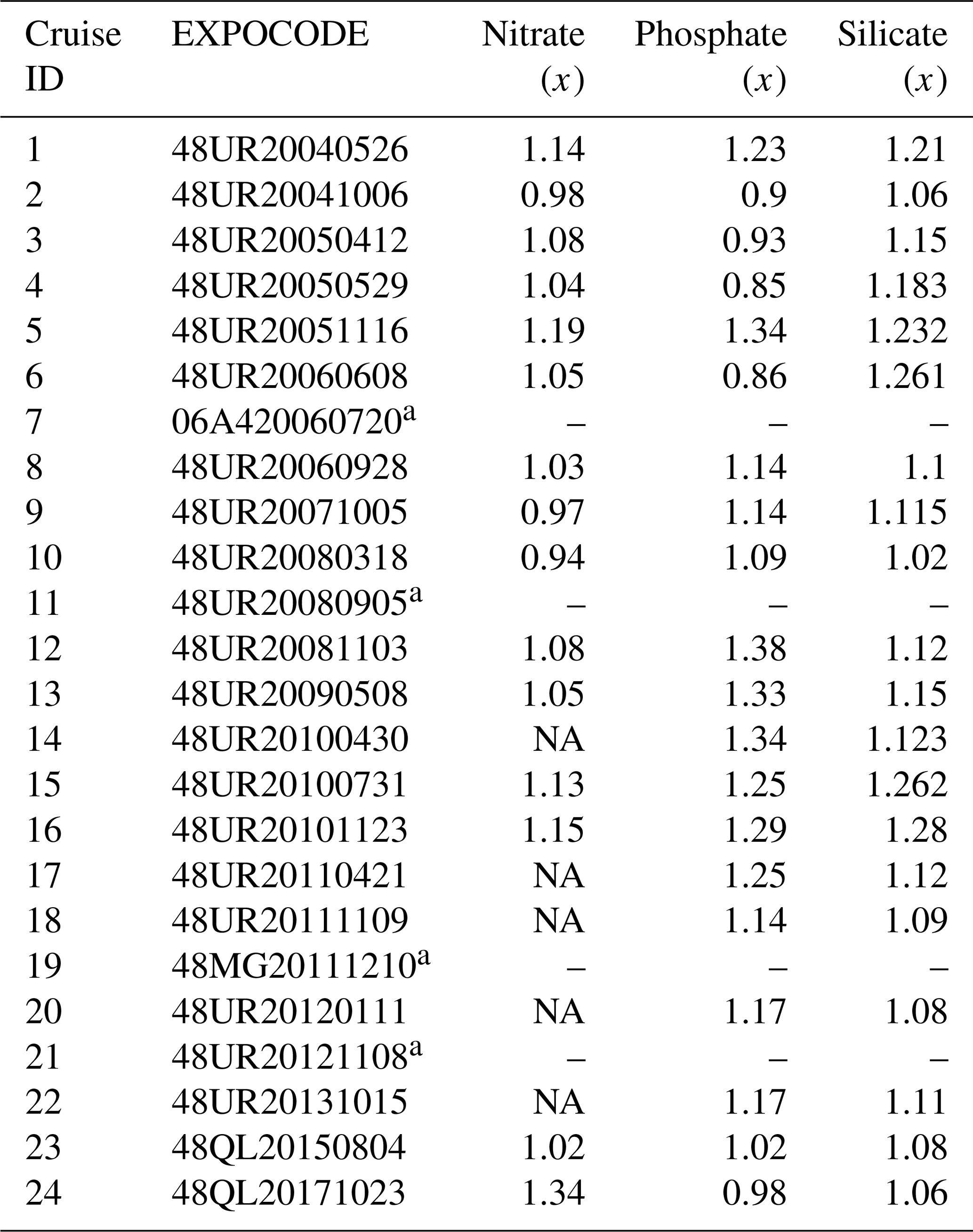
^a Cruise not included in the second QC (Sect. 4.).

Overall, we found a total number of 73 individual crossovers for nitrate, 72 for phosphate, and 54 for silicate. An example of the running cluster crossover output is shown in Fig. 4. Results of the crossover analysis is an adjustment factor for each cruise and each nutrient, which are shown in Table 5 and Figs. 5–7. The adjustment factor was calculated from the weighted mean of the absolute offset summarized in Table 6 and Figs. S3–S5. Table 6 details the improvement of the weighted mean of the absolute offset by cruise prior to and after adjustments; the information is also displayed graphically in Figs. S3–S5. Cruises are in chronological order in all figures and tables.

Table 6 Secondary QC toolbox results: improvements of the weighted mean of absolute offset per cruise of unadjusted and adjusted data; n is the number of crossovers per cruise. The numbers in bold (less than 1) indicate that the cruise data are lower than the reference cruises. NA: not adjusted.

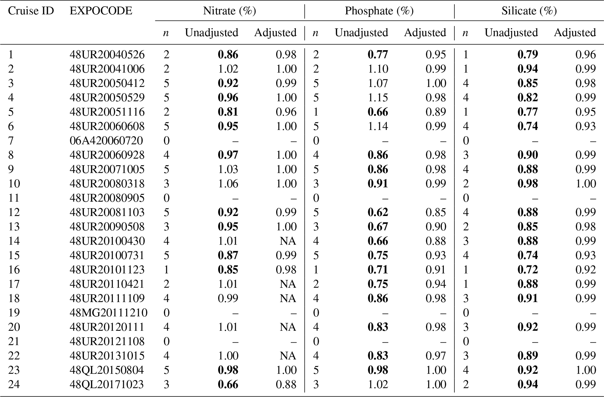
In bold: data lower than reference.

4.1 Nitrate

The crossover analysis suggests a significant adjustment for nitrate concentrations on 15 cruises, between 0.94 and 0.98 (for adjustments <1) and between 1.02 and 1.34 (for adjustments >1; Table 5 and Fig. 5). Offsets suggest that the deep measurements of cruises no. 1, no. 3, no. 4, no. 5, no. 6, no. 8, no. 12, no. 13, no. 15, no. 16, no. 23, and no. 24 need to be adjusted towards higher concentrations when compared to the respective reference (Fig. S3).

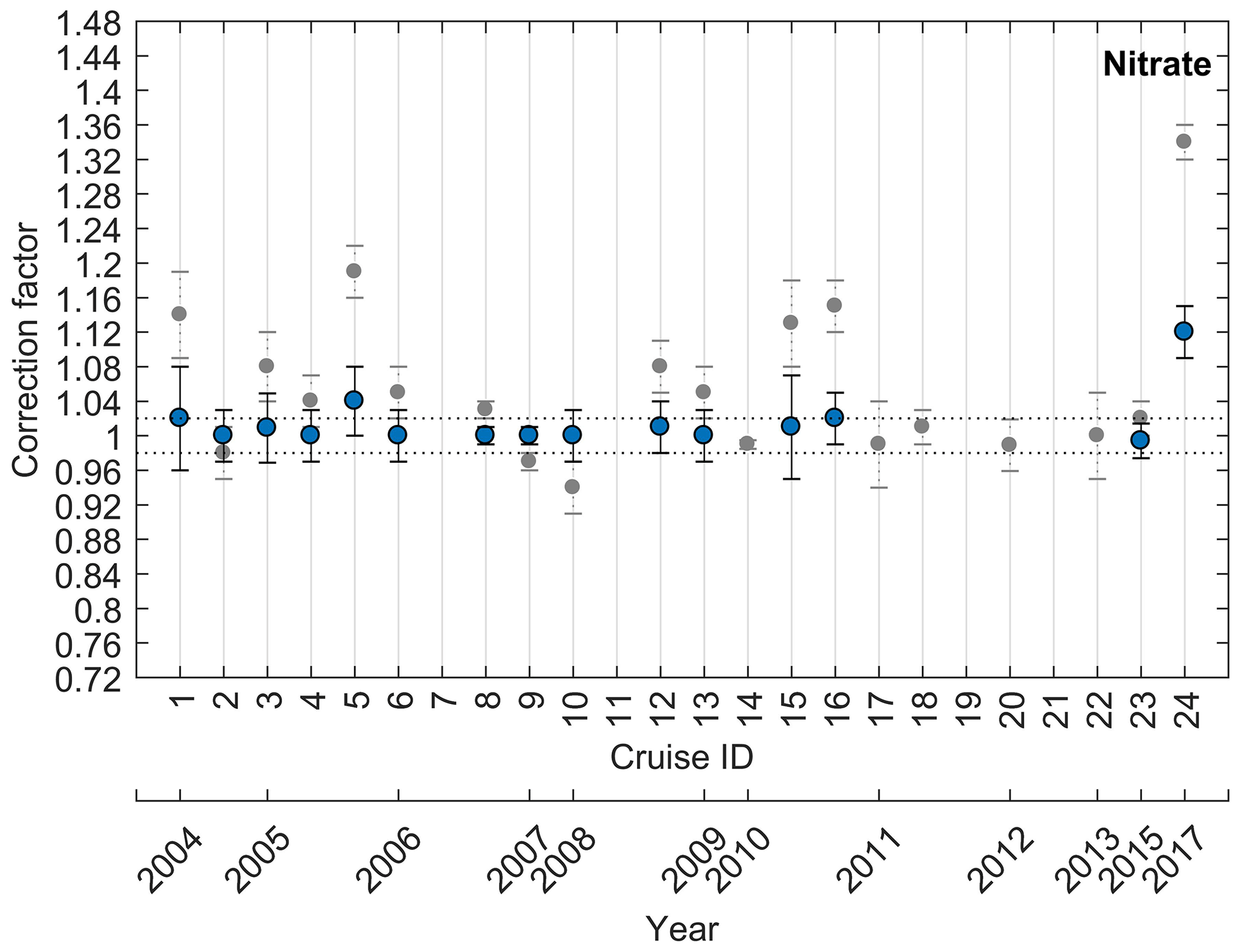
Figure 5 Results of the crossover analysis for nitrate, before (grey) and after (blue) adjustment. Error bars indicate the standard deviation of the absolute weighted offset. The dashed lines indicate the 2 % accuracy limit for an adjustment to be recommended.

Nitrate observations of cruises no. 2, no. 9, and no. 10 on the other hand were higher than the reference cruises and exhibit variation outside the accepted accuracy limit, thus requiring a downward adjustment.

Finally, five cruises (no. 14, no. 17, no. 18, no. 20, and no. 22) were consistent with the reference data and no adjustment was necessary. Considering the weighted mean of absolute offset after adjustments shown in Table 6, two cruises (no. 5 and no. 24) required large correction factors but remain outside the accuracy threshold (Fig. 5). These cruises are considered in detail later (Sect. 4.4).

Figure 6 The same as Fig. 5 but for phosphate.

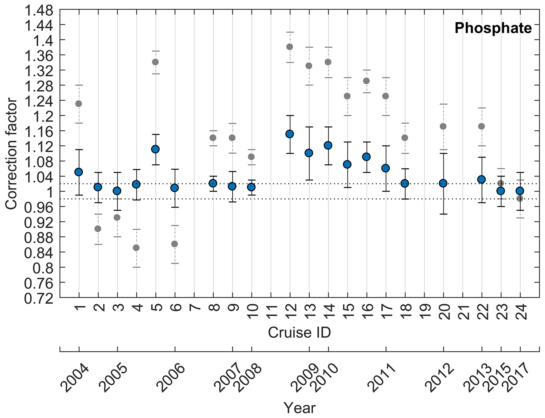
4.2 Phosphate

For phosphate the crossover analysis suggests adjustments for 20 cruises, as shown in Fig. 6. Deep phosphate measurements of 15 cruises (Table 6) appear to be lower than the respective reference measurements (i.e. phosphate data of these cruises require an upward adjustment), while the data of five cruises (no. 2, no. 3, no. 4, no. 6, no. 24) are higher (i.e. they need a downward adjustment; Fig. S4). Applying all the indicated adjustments, the large offsets of cruises no. 2, no. 3, no. 4, no. 6, no. 8, no. 9, no. 10, no. 18, no. 20, no. 23, and no. 24 are reduced and become consistent with the reference. Cruises no. 1, no. 5, no. 12, no. 13, no. 14, no. 15, no. 16, no. 17, and no. 22 retain an offset even after applying the indicated adjustment. These cruises are considered in detail later.

According to Olsen et al. (2016), if a temporal trend is detected in the offsets, no adjustments should be applied. There is indeed a decreasing trend between 2008 and 2017 in the phosphate correction factor (Fig. 6) and thus an increasing one in the weighted mean offset (Fig. S4), implying a temporal increase in phosphate. Therefore, phosphate data of the cruises being part of the trend were not flagged as questionable, except some cruises that are discussed further in Sect. 4.4.

Comparing phosphate before and after adjustment, the corrections did minimize the difference with the reference while the actual variation with time was preserved (Fig. 6). The temporal trend towards higher phosphate concentrations in the Mediterranean Sea is considered to be real, even though studies concerning the biogeochemical trends in the deep layers of the WMED are scarce (Pasqueron et al., 2015). However, this variation could be consistent with the findings of Béthoux et al. (1998, 2002) and the modelling studies by Moon et al. (2016) and Powley et al. (2018), who indeed found an increasing trend in phosphate concentrations over time, due to the increase in the atmospheric and terrestrial inputs.

Figure 7 The same as Fig. 5 but for silicate.

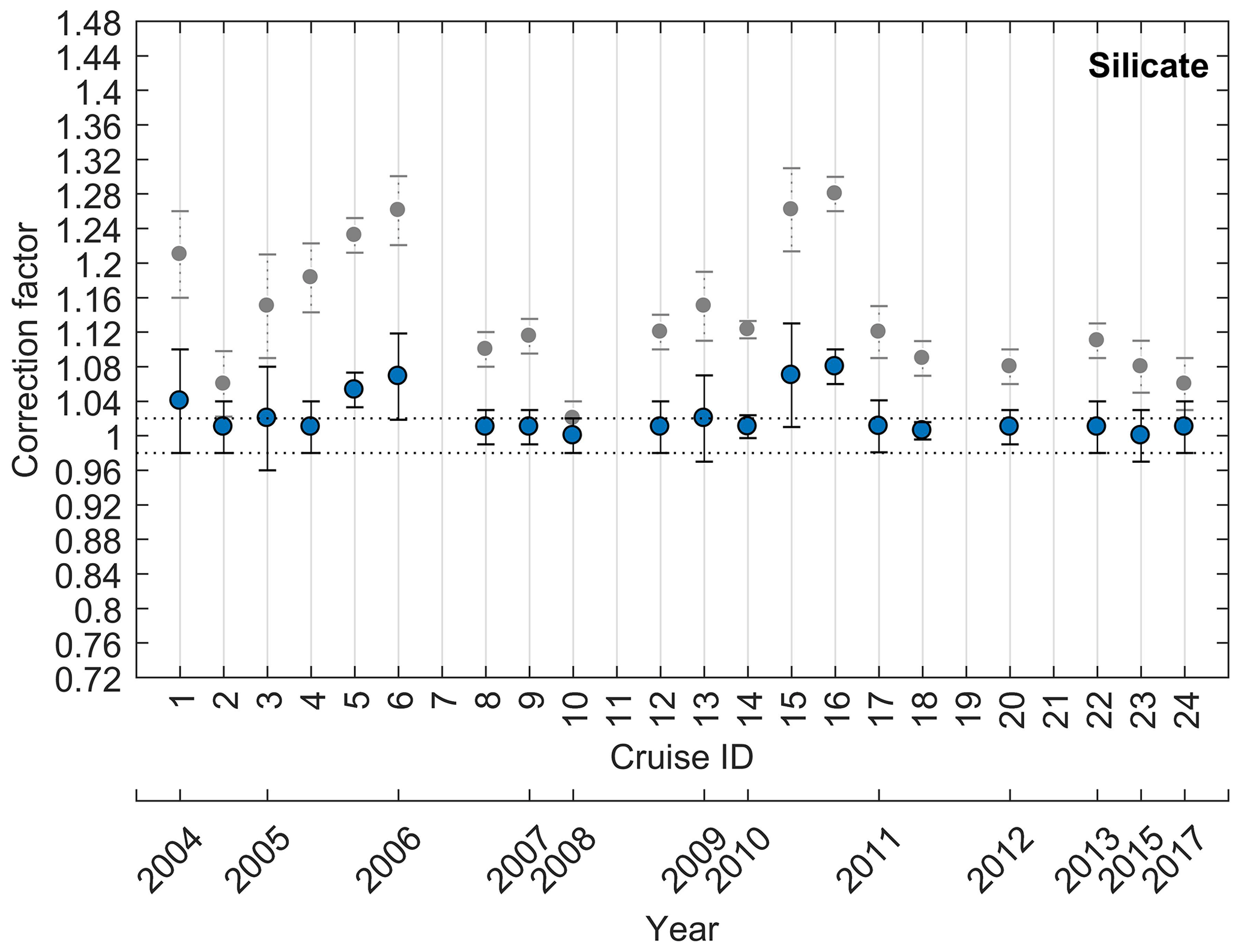
4.3 Silicate

The results of the crossover analysis for silicate suggest corrections for all cruises (Fig. 7). The crossovers indicate that deep silicate measurements are lower in the evaluated cruises than in the corresponding reference cruises (i.e. they need to be adjusted upward; Fig. S5). This is likely to be a direct result of freezing the samples before analysis, since the reactive silica polymerizes when frozen (Becker et al., 2019). After applying the adjustment (Table 5), as expected, the offsets are reduced (Table 6), but five cruises (no. 1, no. 5, no. 6, no. 15, and no. 16) remain outside the accuracy envelope. Due to the large offsets, these cruises will be discussed further in Sect. 4.4.

4.4 Discussion and recommendations

Adjustments were evaluated for each cruise separately. As a general rule, no correction was applied when the suggested adjustment was strictly within the 2 % limit (indicated with NA in Table 5). The average correction factors were 1.06 for nitrate, 1.14 for phosphate, and 1.14 for silicate, respectively. To verify the results, we reran the crossover analysis and recomputed offsets and adjustment factors using the adjusted data (as shown in blue in Figs. S3–S5 and 5–7). Most of the new adjustments are within the accuracy envelope and few are outside the limit, except for the cruises belonging to the above-mentioned phosphate trend and the other outlying cruises which are detailed hereafter. By the application of adjustments, the deep-water offsets were reduced. This can be seen in the decrease in the weighted mean offset between the data before adjustments (after first QC, Figs. S3–S5, in grey) and the adjusted data (after second QC, Figs. S3–S5, in blue).

Referring to the analysis detailed in Sect. 3.2, the internal consistency of the nutrient dataset has improved and increased significantly after the adjustment, from 4 % for nitrate, 19 % for phosphate, and 13 % for silicate to a more unified dataset with 3 % for nitrate, 6 % for phosphate, and 3 % for silicate.

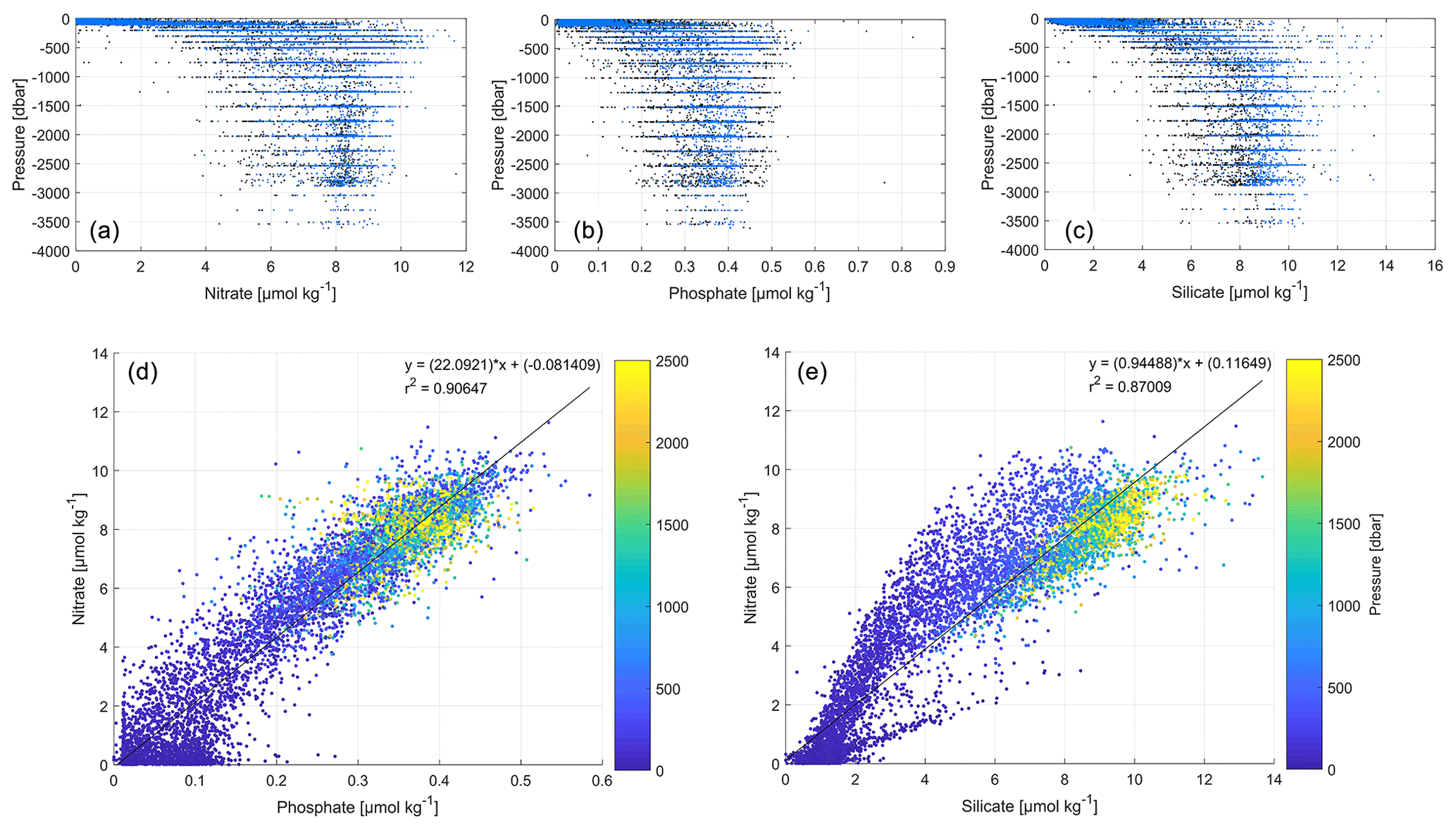
Figure 8 Dataset comparison before (black) and after (blue) adjustment, showing vertical profiles of (a) nitrate (µmol kg⁻¹), (b) phosphate (µmol kg⁻¹), and (c) silicate (µmol kg⁻¹). Scatter plots of the adjusted data from all depths after first and second quality control for (d) phosphate vs. nitrate (µmol kg⁻¹) and (e) silicate vs. nitrate (µmol kg⁻¹). The black lines represent the best linear fit between the two parameters, and the corresponding equations and r² values are shown in each plot. Average resulting N:P ratio is 22.09; average resulting N:Si ratio is 0.94 (whole depth).

A comparison between the original and the adjusted nutrient observations is shown in Fig. 8a–c, indicating an improvement in the accuracy based on the reference data and a relatively reduced range particularly for phosphate (Fig. 8b). Figure 8d–e scatter plots show that after the quality control, nutrient stoichiometry slopes obtained from regressions, between tracers along the water column, demonstrate a strong coupling and provide a nitrate-to-phosphate ratio of ∼22.09 and a nitrate-to-silicate ratio of ∼0.94. These values are consistent with nutrient ratio ranges found in the WMED as reported in Lazzari et al. (2016), Pujo-Pay et al. (2011), and Segura-Noguera et al. (2016). The regression model is more accurate after adjustments with an improved r² for N:P (from 0.81 to 0.90) and for N:Si (from 0.85 to 0.87).

In the following some details on the adjustment of specific cruises are given.

Cruise no. 2 (48UR20041006) needed an adjustment of 0.98 for nitrate, 0.9 for phosphate, and 1.06 for silicate. Most of the crossover profiles occur in the Tyrrhenian Sea (Tyrrhenian North and Tyrrhenian South subregions). After adjustment, the cruise is inside the 2 % envelope.

Cruise no. 3 (48UR20050412) appeared to be outside the 2 % envelope before adjustments. Its offsets with five reference cruises, crossing the Tyrrhenian Sea, Sardinia Channel, Gulf of Lion, and Algero-Provençal subregions, showed nitrate and silicate values to be relatively low, and thus an adjustment of 1.08 and 1.15 was applied, respectively. On the other hand, phosphate values were relatively high, and a 0.93 adjustment was applied.

The cruise no. 4 (48UR20050529) correction factor estimate was based on five crossovers that covered five subregions: the Tyrrhenian South, Sardinian Channel, Algerian East and West, and Alboran Sea. Table 4 shows that there are no large differences between regional averages within the cruise which justify an adjustment of 1.04 for nitrate, 0.85 for phosphate, and 1.183 for silicate.

Cruise no. 8 (48UR20060928) was adjusted by 1.03 for nitrate, 1.14 for phosphate, and 1.1 for silicate, because it showed values to be low compared to four references. After adjustment, the data were inside the acceptable range.

Cruise no. 9 (48UR20071005) values of nitrate were slightly outside the 2 % envelope before adjustments, similar to phosphate and silicate which were lower compared to the reference. The adjustments of 0.97 for nitrate, 1.14 for phosphate, and 1.115 for silicate suggested by the mean offset against the reference cruises were recommended.

Cruise no. 10 (48UR20080318) has only three crossovers in the Algero-Provençal subregion, showing that nitrate is too high compared to the reference, while phosphate and silicate are slightly lower. We therefore applied the adjustments of Table 5, since the deep averages in each region (Table 4) did not show large regional differences.

Cruise no. 13 (48UR20090508) has three crossovers in the common crossing zone that included the Tyrrhenian North, Tyrrhenian South, and Sardinia Channel subregions. The crossover suggests that this cruise has too low values and needs an adjustment of 1.05 for nitrate, 1.33 for phosphate, and 1.15 for silicate.

Cruise no. 14 (48UR20100430) has a mean offset with four reference cruises that suggests an adjustment factor of 1.34 for phosphate and 1.123 for silicate. Nitrate fell within the accuracy envelope; no adjustment was needed.

Cruise no. 17 (48UR20110421) crossover analysis did not suggest any correction for nitrate; however, with an offset based on two crossovers in the Tyrrhenian North and South subregions, adjustments were recommended for phosphate (1.25) and silicate (1.12), for being lower than the reference cruises.

Cruise no. 18 (48UR20111109) is similar to cruise no. 17, since it was suggested to adjust phosphate by 1.14 and silicate by 1.09, based on four crossovers in the Tyrrhenian North and South, Sardinia Channel, and Algero-Provençal subregions.

Cruise no. 20 (48UR20120111) has four crossovers over the Tyrrhenian North and South and Algero-Provençal subregions. Its measurements were slightly lower than the reference cruises, suggesting a correction factor of 1.17 for phosphate and 1.08 for silicate.

Cruise no. 22 (48UR20131015) has similar correction factors to cruise no. 20, based on three crossovers in the Sardinia Channel and Tyrrhenian North and South subregions, with measurements being lower than the reference.

Cruise no. 23 (48QL20150804) showed nutrient values slightly lower than the reference cruises as well, suggesting small correction factors of 1.02 for both nitrate and phosphate and 1.08 for silicate, correction factors that were based on offsets with five cruises.

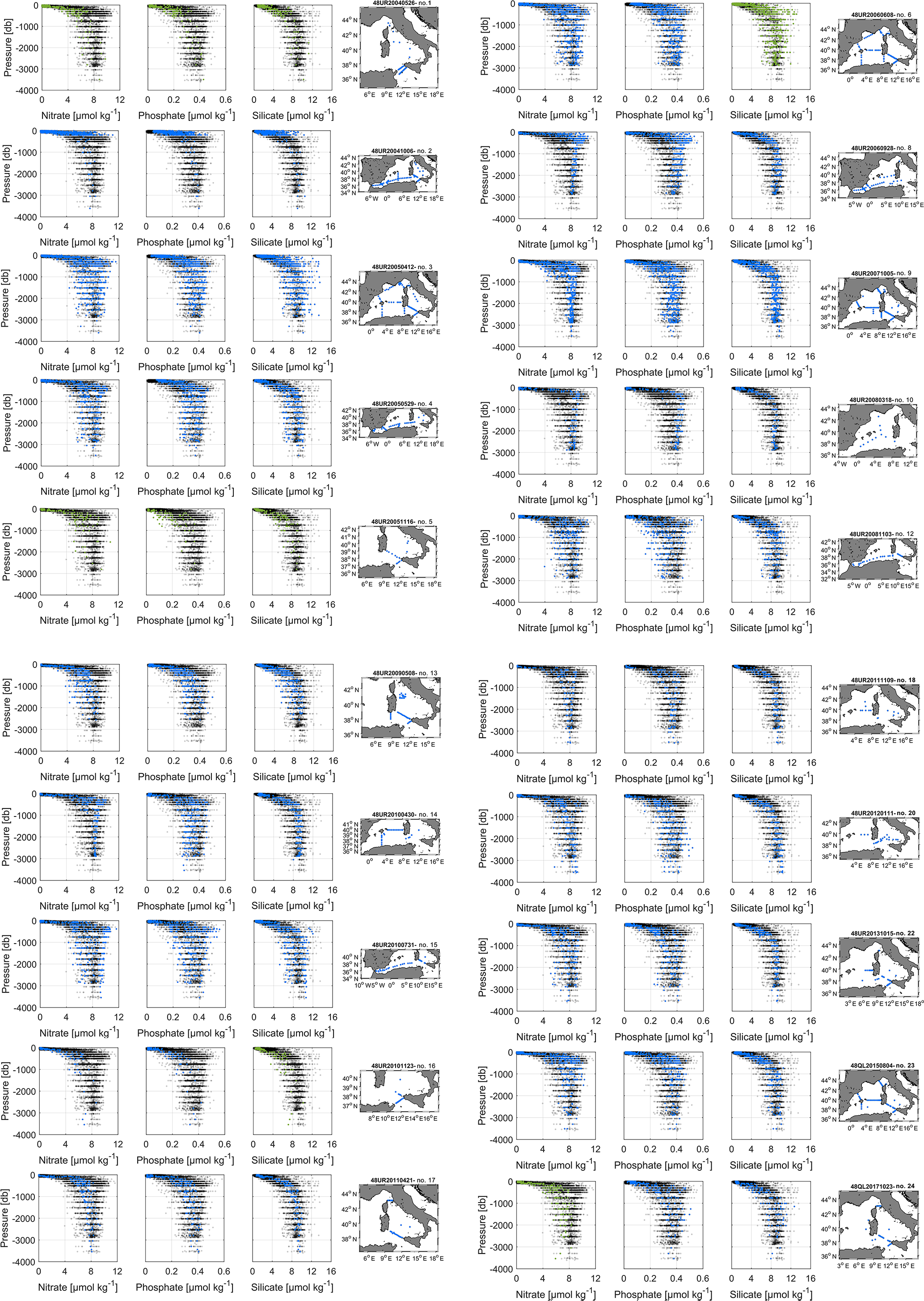
Figure 9 Vertical profiles of the inorganic nutrients in the dataset after adjustments and spatial coverage of each cruise (reference to cruise ID is above each map). The whole WMED adjusted product is shown in black, while the data of each individual cruise are shown in blue (flag 2) and green (flag 3).

Below, we discuss the recommended flags in the final product (Table 3; see Supplement Part 2, A2) assigned for some cruises that needed further consideration, since they required larger adjustment factors:

Cruise no. 1 (48UR20040526). The adjusted values are still lower than the reference (Figs. 5–7, S3–S5) and are still outside the 2 % accuracy range. This cruise had stations in the Strait of Sicily, Tyrrhenian North and South, and Ligurian East subregions (Fig. 9, right side), and only four stations were deeper than 1000 db (those within the Tyrrhenian Sea). The low precision of this cruise had already been evidenced during the first QC (Sect. 3.1). We recommend flagging this cruise as questionable (flag 3).

Cruise no. 5 (48UR20051116). This cruise took place between the Strait of Sicily and the Tyrrhenian North and South (Fig. 9, right side). Nitrate, phosphate, and silicate data were lower than those from other cruises (no. 3 and no. 4) run the same year (Figs. 5–7, S3–S5) and are still biased after adjustments. Considering the limited precision and the low number of crossovers, it is recommended to flag the cruise as questionable (flag 3).

Cruise no. 6 (48UR20060608). This cruise had an offset with five cruises, giving evidence that adjustments of 1.05 for nitrate, 0.86 for phosphate, and 1.26 for silicate are needed. The silicate bias was reduced after adjustment but remained large with respect to the accuracy limit (Figs. 7, S5). This cruise has a wide geographic coverage, with stations along nine sections (Fig. 9, right side). Considering also the high standard deviation (Table 4), which is partially attributed to the spatial coverage of the cruise, there is still uncertainty about the quality of the samples. It is recommended to flag silicate data of cruise no. 6 as questionable (flag 3).

Cruise no. 12 (48UR20081103). Phosphate data have low accuracy with respect to the reference cruises (Figs. 6, S4). This cruise has stations along a longitudinal section from the Strait of Sicily to the Alboran Sea, which might explain the large standard deviation of deep phosphate samples (Table 4). Cruise no. 12 was given a correction of 1.08 for nitrate, 1.12 for silicate, and 1.38 for phosphate. The mean offset from five crossovers computed within the Tyrrhenian South, Sardinia Channel, Algerian East, Algerian West, and Alboran Sea subregions suggests that this cruise has lower nutrient values than the reference cruise. After adjustment, cruise no. 12 is within the acceptable range for nitrate and silicate but not for phosphate as highlighted in Sect. 3.2. In addition, considering the relatively high number of stations >1000 db and a plausible trend in phosphate, it is recommended to flag the phosphate data as good/acceptable (flag 2).

Cruise no. 15 (48UR20100731). This cruise has 149 stations along a similar track to cruise no. 12 but shows larger offsets for phosphate and silicate (Figs. 6–7, S4–S5) compared to cruise no. 12. Considering that deep silicate data were not of low quality (small standard deviation; see Table 4) and that deep phosphate data fall within the phosphate trend discussed above, these data are flagged as good/acceptable (flag 2).

Cruise no. 16 (48UR20101123). The cruise shows large offsets for phosphate and silicate (Figs. 6–7, S4–S5), similar to cruise no. 15. Considering that the overall cruise standard deviation of silicate samples below 1000 db was relatively high (1.02 over 14 samples; see Table 4); that it has only one crossover between the Tyrrhenian North and South subregions (Table 6); and that when comparing deep regional averages, this cruise had the lowest average silicate value, it is recommended to flag silicate data of cruise no. 16 as questionable (flag 3). As for phosphate, the cruise is part of the phosphate trend and is therefore flagged as good/acceptable (flag 2).

Cruise no. 24 (48QL20171023). This cruise has the largest offset for nitrate even after adjustment. It is very likely due to a difference between laboratories (calibration standards) concerning nitrate, which needs to be flagged as questionable (flag 3) in the final product.

There are several sources of bias in the observation. One of the main reasons for an upward or downward bias would be the difference in the nutrient's chemical analytical method and the lack of use of CRMs in all cruises as also noted in CARINA (Tanhua et al., 2009) or in the most recent global comparability study by Aoyama (2020).

Cruises discussed in this section were not removed from the final product but were retained along with their recommended quality flag (Table 3), detailed above and in the Supplement – Part 2, A2. We have carried out the evaluation of their overall quality but leave up to the users how to appropriately use these data.

Table 7 Water mass properties and regional average concentrations of inorganic nutrients: comparison between the new adjusted product and the MEDAR/MEDATLAS climatology (with standard deviations and number of observations in brackets).

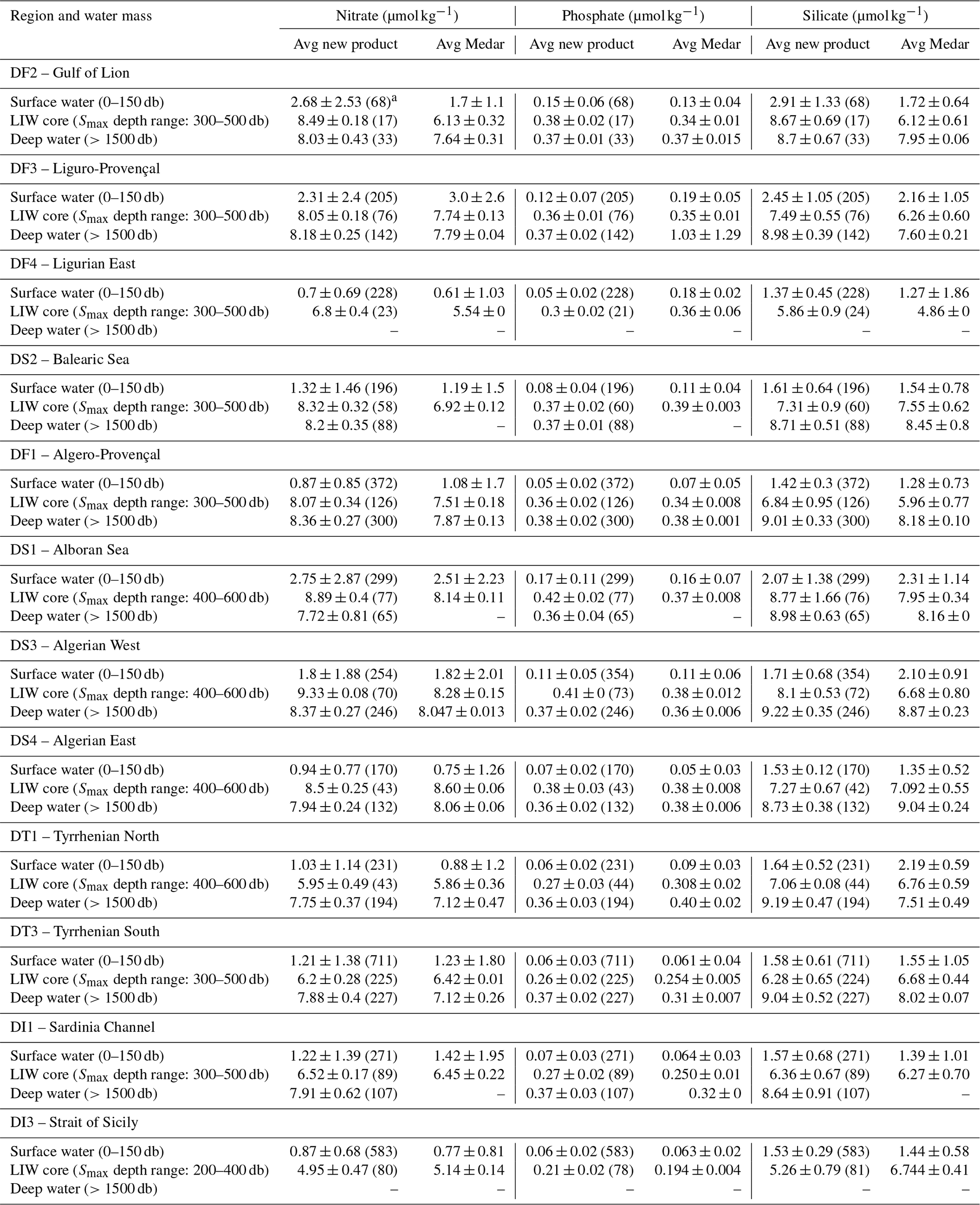
^a Average (Avg) ± standard deviation of inorganic nutrients (the number of observations within depth range) for three layers from the adjusted or new product and MEDATLAS vertical climatological profiles (called here Medar). Regions are defined according to Manca et al. (2004; Table S2, Fig. S2).

4.5 Product assessment – comparison with MEDATLAS

Average water mass biogeochemical properties have been computed from the adjusted product (Table 7) and compared to the MEDAR/MEDATLAS annual climatological profiles, downloaded from the Italian National Oceanographic Data Centre (NODC) website (http://doga.ogs.trieste.it/medar/, last access: February 2020) given by Manca et al. (2004), in order to evaluate and assess the new product. Since nutrient properties exhibit differences with depths, we compared average nutrient concentrations of the three main water masses in 12 subregions of the WMED (Table 7, Fig. S2).

The results of Table 7 compare water mass biogeochemical properties with the reference climatology. The new product agrees well with the MEDATLAS climatology. However, there are some distinctions. The surface layer (0–150 db) is characterized by a low nutrient content. The surface nitrate varies between 0.69 and 2.75 µmol kg⁻¹ with a maximum found in the Ligurian East (DF4) and a minimum in the Alboran Sea (DS1) subregions; similar values were recorded in the climatology (0.61–3.00 µmol kg⁻¹). The differences in nitrate averages in the surface layer are observed in the Gulf of Lion (DF2) where the new product is higher than the climatology and slightly lower in the Liguro-Provençal (DF3). As for the surface content in phosphate, it varied between 0.04 and 0.16 µmol kg⁻¹ with a maximum found in the Ligurian East (DF1) and a minimum in the Alboran Sea (DS1), like the MEDATLAS climatology, where phosphate averages fluctuate between 0.05 and 0.19 µmol kg⁻¹. The new product is slightly lower compared to the climatology. As to the average surface in silicate, it varies between 1.36 and 2.91 µmol kg⁻¹ with a minimum found in the Ligurian East (DF4) and a maximum in the Gulf of Lion (DF2), while in the climatology, it varied between 1.27 and 2.31 µmol kg⁻¹ (the minimum in the Ligurian East – DF4 – and the maximum in the Alboran Sea – DS1). The new product is slightly higher in silicate.

Overall, the differences in the surface layer are observed in the Gulf of Lion (DF2), the Liguro-Provençal (DF3), and the Ligurian East (DF4) regions which could be due to the intense variability of the vertical mixing occurring in the northern WMED compared to in the other subregions.

In the intermediate layer, averages were computed from the depth of the salinity maximum (S_max)±100 m from a regional average profile, indicative of the Levantine Intermediate Water (LIW) core. The nitrate average varied between 4.94 and 9.32 µmol kg⁻¹ where the minimum content was recorded in the Strait of Sicily (DI3) and the maximum in the Algerian West, (DS3) while in the MEDATLAS climatology, nitrate was between 5.14 and 8.60 µmol kg⁻¹. On average, the lowest content in nitrate was in the Tyrrhenian North (DT1) and South (DT3), Sardinia Channel (DI1), and Strait of Sicily (DI3), while LIW of the Gulf of Lion (DF2), Liguro-Provençal (DF3), Ligurian East (DF4), Balearic Sea (DS2), Algero-Provençal (DF1), Alboran Sea (DS1), and Algerian West (DS3) and East (DS4) subregions was relatively rich in nitrate compared to the MEDATLAS product, though the new product was slightly higher mainly in the Gulf of Lion (DF2), Ligurian East (DF4), and Balearic Sea (DS2). As for phosphate, LIW averages showed similar behaviour to nitrate: the lowest phosphate content (0.21–0.27 µmol kg⁻¹) was observed in the eastern subregions of the WMED (DI3, DI1, DT3, and DT1), while the maximum concentrations (0.4–0.37 µmol kg⁻¹) were reported in the western subregions of the WMED (DS1, DS3 and DS4, DS2, and DF2). The large differences between the two products were in the Ligurian East (DF4) and the Alboran Sea (DS1), subregions with low numbers of observations.

Concerning silicate, the lowest average concentration (5.25 µmol kg⁻¹) was observed in the LIW core of the Strait of Sicily (DI3) and the maximum concentrations (8.66–8.77 µmol kg⁻¹) were in the Alboran Sea (DS1) and Gulf of Lion (DF2); similar values were recorded in the MEDATLAS climatology (4.86–7.95 µmol kg⁻¹). There are some discrepancies where the new product was higher particularly in the Gulf of Lion (DF2), Liguro-Provençal (DF3), and Algerian West (DS3) subregions. This difference is explained by the limited number of observations within the depth range in the new product compared to the observations used in the climatology in these subregions.

Referring to Manca et al. (2004), the LIW core salinity values are relatively more pronounced in the Strait of Sicily (DI3), Sardinia Channel (DI1), and Tyrrhenian South (DT3) and North (DT1) subregions, where nutrients were lower than in the western subregions (DS3, DS4, DS1, DF1, DS2, DF4, DF3, DF2). The averages of nutrient within the LIW core tie in well with the MEDATLAS climatology averages (Table 7), except in subregions with important vertical mixing.

We have also verified average biochemical properties in the deep layer (below 1500 db). The new product is slightly higher in nitrate averages (7.74–8.37 µmol kg⁻¹) than the MEDATLAS climatology (7.12–8.06 µmol kg⁻¹; Table 7). The largest difference was found in the Tyrrhenian South (DT3) and North (DT1) subregions. This difference could be due to the fact that we are comparing two different time periods (2004–2017 and 1908–2001). As for the deep layer phosphate, average concentrations varied between 0.35 and 0.37 µmol kg⁻¹ and were within the climatology limits (0.31–0.40 µmol kg⁻¹). In all subregions, there were not large differences. Overall, phosphate was in accordance with the MEDATLAS climatology. Similarly to nitrate, deep average silicate in the new product (8.64–9.21 µmol kg⁻¹) was higher than the climatology (7.51 to 9.04 µmol kg⁻¹). The largest difference in average silicate was observed in the Tyrrhenian North (DT1) and South (DT3) and Liguro-Provençal (DF3) subregions.

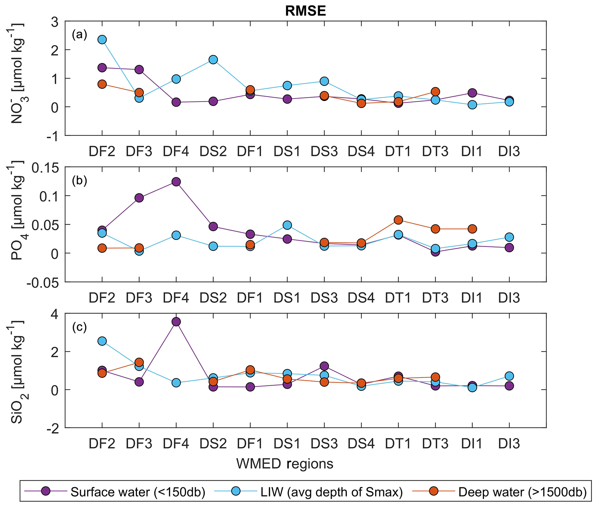
Figure 10 RMSE regional averages of water mass properties computed between the new adjusted product and MEDAR/MEDATLAS climatology for nitrate (a), phosphate (b), and silicate (c).

We then used the root mean square error (RMSE) as a statistical index to quantify the difference between averaged regional profiles from the new product and MEDATLAS product. The climatology annual profiles were interpolated to the regional average profiles of the new product, and the average RMSE for each layer and subregion was calculated. Figure 10 shows the regional evolution of RMSE in the main water masses for the three nutrients. For nitrate (Fig. 10a), the RMSE in the surface layer varied between 0.12 µmol kg⁻¹ (in the Tyrrhenian North – DT1) and 1.36 µmol kg⁻¹ (in the Gulf of Lion – DF2); in the intermediate layer, the RMSE was between 0.07 µmol kg⁻¹ (in the Sardinia Channel – DI1) and 2.35 µmol kg⁻¹ (in the Gulf of Lion – DF2) and was lower in the deep layer, between 0.11 µmol kg⁻¹ (in the Algerian East – DS4) and 0.79 µmol kg⁻¹ (the Gulf of Lion – DF2). The RMSE decreases in the Algerian East (DS4), Tyrrhenian North (DT1), Tyrrhenian South (DT3), Sardinia Channel (DI1), and Strait of Sicily (DI3). This illustrates the low difference between the two products.

For phosphate (Fig. 10b), the RMSE ranges between 0.0022 µmol kg⁻¹ (in the Tyrrhenian South – DT3) and 0.12 µmol kg⁻¹ (in the Ligurian East – DF4) in the surface layer and is between 0.003 µmol kg⁻¹ (in the Liguro-Provençal subregion – DF3) and 0.048 µmol kg⁻¹ (in the Alboran Sea – DS1) at intermediate depths, while in the deep layer RMSE varied between 0.0087 (in the Gulf of Lion – DF2) and 0.057 µmol kg⁻¹ (in the Tyrrhenian North – DT1).

Regarding silicate RMSE (Fig. 10c) in the surface layer, it varied between 0.13 µmol kg⁻¹ (in the Algero-Provençal subregion – DF1) and 3.5 µmol kg⁻¹ (in the Ligurian East subregion – DF4); a lower RMSE of between 0.10 µmol kg⁻¹ (in the Sardinia Channel – DI1) and 2.54 µmol kg⁻¹ (in the Gulf of Lion – DF2) was reported in the intermediate layer; the results in the deep layer were between 0.33 µmol kg⁻¹ (in the Algerian East – DS4) and 1.43 µmol kg⁻¹ (in the Liguro-Provençal subregion – DF3).

The best agreement between the two products was observed in the intermediate and deep layer. The lowest RMSE was confined to the deep layer in most of the subregions, while the highest difference was found in the surface layer since it is subjected to intense vertical mixing mainly in the northern WMED. Comparing averages in subregions showed similar differences in nutrients between the two products particularly in the Gulf of Lion (DF2), the Liguro-Provençal (DF3), Ligurian East (DF4), and Algerian East (DS4), due to the relatively high variability in nutrient concentrations in these subregions. These differences are not significant as there is a discrepancy in the number of observations used in the two products. Overall, inorganic nutrients of the new product agree very well with the MEDAR/MEDATLAS climatology. The main features of the spatial distribution in the inorganic nutrients were in accordance with the findings of Manca et al. (2004), where the relatively high content in nutrients was found more in the intermediate layer of the Algerian subregions (DF1, DS3, DS4) than in other subregions (Table 7). Besides, the highest concentrations in deep-layer silicate were reported in the Algerian subregions in the two products (9.21 µmol kg⁻¹ – DS3 – in the new product; 9.04 µmol kg⁻¹ – DS4 – in the climatology), which is indicative of the poor regional ventilation and of the longer residence time of deep water especially in these subregions.

5 Data availability

The final product is available as a *.csv merged file from PANGAEA and can be accessed at https://doi.org/10.1594/PANGAEA.904172 (Belgacem et al., 2019).

Ancillary information is in the supplementary materials with the list of variables included in the original and final product. Table 1a and b summarizes all cruises included in the dataset. The dataset includes frequently measured stations and key transects of the WMED with in situ physical and chemical oceanographic observations. As mentioned, two files are accessible; both include oceanographic variables observed at the standard depths (see Supplement Part 2).

Original dataset – CNR_DIN_WMED_20042017_original.csv. This is the original dataset with a flag variable for each of the following parameters: CTD salinity, nitrate, phosphate, and silicate from the primary quality control (detailed in Sect. 3.1).

Adjusted dataset – CNR_DIN_WMED_20042017_adjusted.csv. This is the product after primary quality control and after applying the adjustment factors from the secondary quality control. Recommendations of Sect. 4.4 are included, as well as quality flags.

6 Final remarks

An internally consistent dataset of dissolved inorganic nutrients has been generated for the WMED (2004–2017). The accuracy envelope for nitrate and silicate was set to 2 %, a predefined limit used in GLODAP and CARINA data products. Regarding phosphate data, these were almost entirely outside this limit, because of phosphate's natural variations and the overall very low concentrations in the WMED, a highly P-limited basin. Using a crossover analysis (second QC toolbox) to compare cruises with respect to reliable reference data improved the accuracy of the measurements by minimizing the bias in the individual cruises. The new product was broadly consistent with the earlier climatology of MEDAR/MEDATLAS.

The publication of a quality-controlled extensive (spatially and temporally) database of inorganic nutrients in the WMED was timely and fills a gap in information that prevented baseline assessments on spatial and temporal variability of biogeochemical tracers in the Mediterranean. In combination with older databases in the same region (e.g. bottle data available in the MEDAR/MEDATLAS database), this new data product will thus constitute a pillar on which the Mediterranean marine scientific community will be able to build with original research topics on biogeochemical fluxes and cycles and their relation to hydrological changes that occurred in the period covered by the dataset. The dataset is also relevant for the modelling community as it can be used as an independent data product to assess reanalysis products or it can be assimilated in new reanalysis products.