the Creative Commons Attribution 4.0 License.
the Creative Commons Attribution 4.0 License.
 | 03 Aug 2020
A multi-year time series of observation-based 3D horizontal and vertical quasi-geostrophic global ocean currents
Bruno Buongiorno Nardelli
Estimates of 3D ocean circulation are needed to improve our understanding of ocean dynamics and to assess their impact on marine ecosystems and Earth climate. Here we present the OMEGA3D product, an observation-based time series of (quasi-)global 3D ocean currents covering the 1993–2018 period, developed by the Italian Consiglio Nazionale delle Ricerche within the European Copernicus Marine Environment Monitoring Service (CMEMS). This dataset was obtained by applying a diabatic quasi-geostrophic (QG) diagnostic model to the data-driven CMEMS-ARMOR3D weekly reconstruction of temperature and salinity as well as ERA Interim fluxes. Outside the equatorial band, vertical velocities were retrieved in the upper 1500 m at 1∕4∘ nominal resolution and successively used to compute the horizontal ageostrophic components. Root mean square differences between OMEGA3D total horizontal velocities and totally independent drifter observations at two different depths (15 and 1000 m) decrease with respect to corresponding estimates obtained from zero-order geostrophic balance, meaning that estimated vertical velocities can also be deemed reliable. OMEGA3D horizontal velocities are also closer to drifter observations than velocities provided by a set of reanalyses spanning a comparable time period but based on data assimilation in ocean general circulation numerical models.
The full OMEGA3D product (released on 31 March 2020) is available upon free registration at https://doi.org/10.25423/cmcc/multiobs_glo_phy_w_rep_015_007 (Buongiorno Nardelli, 2020a). The reduced subset used here for validation and review purposes is openly available at https://doi.org/10.5281/zenodo.3696885 (Buongiorno Nardelli, 2020b).
- Article
(8088 KB) - Full-text XML
- BibTeX
- EndNote


The recognition of the key role played by the oceans in the Earth system led the United Nations to proclaim the Decade of Ocean Science for Sustainable Development (2021–2030). Major efforts will consequently be made in the next years to analyse state-of-the-art observations and models and provide the indispensable knowledge basis to preserve the marine environment through effective, science-informed policies. Providing accurate reconstructions of 3D ocean circulation time series is a fundamental part of this effort, aimed at better describing ocean dynamics and assessing their responses and feedbacks to natural and anthropogenic pressures. However, assessing the time-evolving lateral and vertical transport of energy, momentum, gases, nutrients, marine organisms and pollutants would require repeated synoptic observations of the 3D ocean state and surface forcings that cannot be presently achieved even with the most advanced technologies. Hence, a combination of measurements collected from in situ and remote-sensing platforms and proper modelling frameworks is needed to describe the ocean circulation both in the ocean interior and at the domain boundaries. Two main complementary approaches can be followed to this end: the assimilation of observations in global ocean circulation numerical models (Carrassi et al., 2018; Moore et al., 2019; Stammer et al., 2016) and the combination of diagnostic models and purely data-driven reconstructions. The latter is presently more widely used for surface circulation retrievals, but its extension to 3D ocean state reconstruction is generating growing interest as advanced statistical and machine learning tools are becoming more computationally efficient (Buongiorno Nardelli et al., 2012; Buongiorno Nardelli and Santoleri, 2005; Guinehut et al., 2012; Lopez-Radcenco et al., 2018; Mulet et al., 2012; Rio et al., 2016; Ubelmann et al., 2015; Yan et al., 2020). Both approaches present advantages and drawbacks: data assimilation in prognostic models may guarantee a description of the ocean state evolution that is fully consistent with the physics represented by the model, but the uncertainties in its initialization, the limits of the parameterizations of unresolved processes and the difficulties to properly represent model and observation errors and to account for their representativeness can significantly reduce models' ability to reproduce non-assimilated observations. Conversely, synergic use of satellite in situ observations and data-driven reconstruction methodologies, in combination with simpler dynamical models (often limited to zero-order balances, as in the retrieval of geostrophic currents from sea level data), can provide snapshots that better match independent observations (Mulet et al., 2012; Rio et al., 2016; Ubelmann et al., 2016).
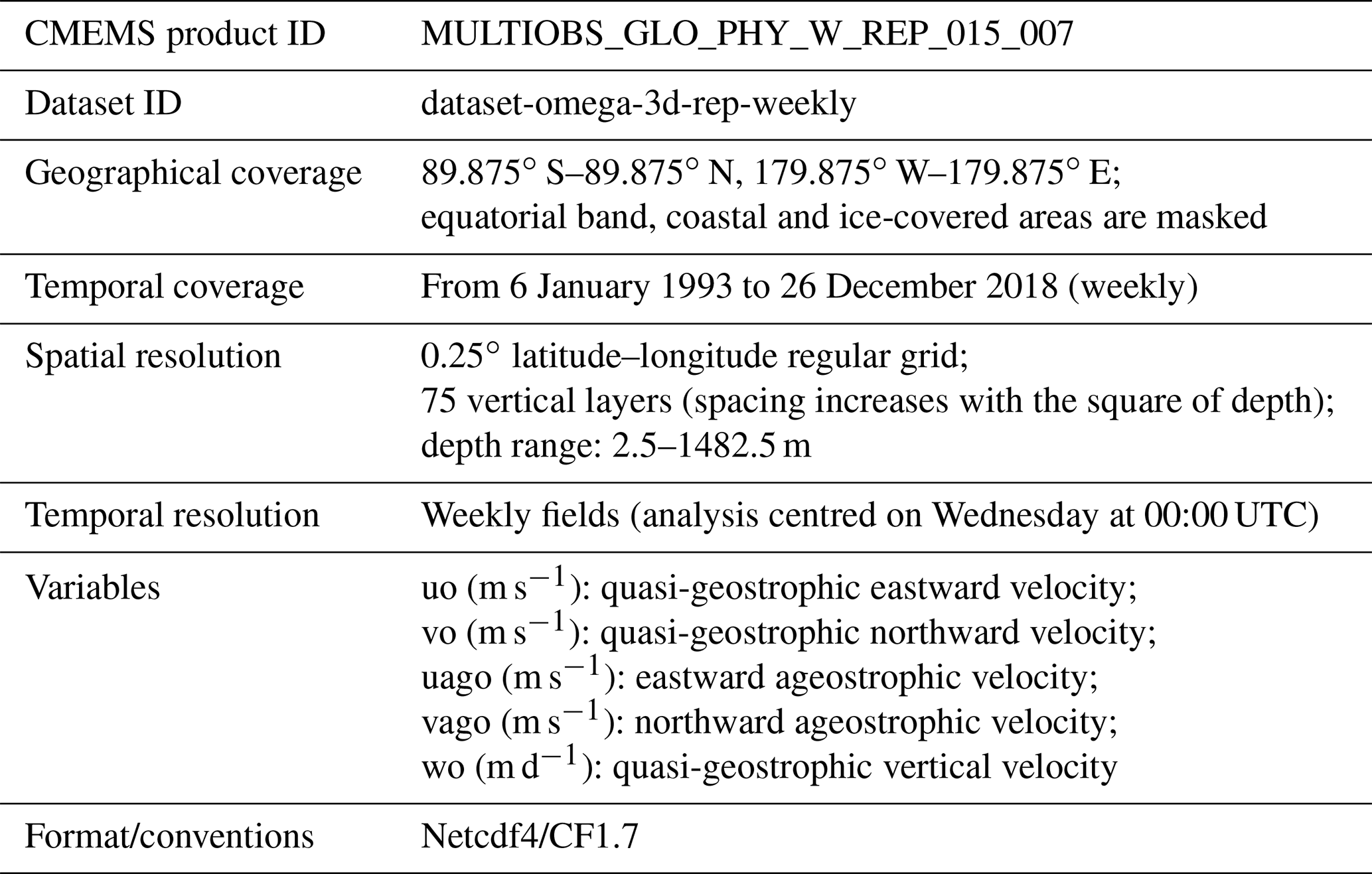
The OMEGA3D product, developed by the Consiglio Nazionale delle Ricerche within the European Copernicus Marine Environment Monitoring Service (CMEMS; http://marine.copernicus.eu/services-portfolio/access-to-products/, last access: 23 July 2020; product ID: MULTIOBS_GLO_PHY_W_REP_015_007), delivers the first observation-based retrievals of the global 3D vertical and horizontal ocean currents computed with a quasi-geostrophic (QG) model that explicitly considers the effect of both geostrophic advection and upper-layer turbulent mixing. The data are provided weekly at 0.25∘ latitude–longitude resolution, with 75 non-uniformly spaced vertical levels between the surface and 1500 m depth, covering the period from January 1993 to December 2018 (with planned yearly extensions based on updated upstream datasets). Outside the equatorial band, vertical velocities are obtained by solving a diabatic Q vector formulation of the QG omega equation (Buongiorno Nardelli et al., 2018b; Giordani et al., 2006), with vertical mixing parameterized through the K-profile parameterization (KPP; Smyth et al., 2002). Only once vertical velocities are known can the horizontal ageostrophic components be retrieved.
The accuracy of the QG velocities depends on the input data and on the theoretical limits of the model and parameterization used. Omega forcings are estimated here from the multi-year CMEMS product ARMOR3D (Guinehut et al., 2012), providing a statistical reconstruction of 3D temperature and salinity fields from a combination of in situ profiles and satellite observations of sea surface temperature, salinity and topography. ERA Interim air–sea fluxes are used to evaluate the forcing terms due to vertical mixing (Dee et al., 2011). QG approximation implies that the omega equation cannot be solved at the Equator, and increased errors are expected in the low-latitude bands.
A direct validation of the vertical velocities is not possible due to the lack of direct reference observations. As such, OMEGA3D vertical velocity mean pattern and variability have been compared here with two global model reanalyses that include vertical velocity fields as disseminated output, namely Estimating the Circulation and Climate of the Ocean (ECCO; Forget et al., 2015) and Simple Ocean Data Assimilation (SODA; Carton et al., 2018).
Total horizontal and geostrophic components are instead compared with fully independent velocity estimates obtained from drifting-buoy and Argo float displacement. For reference, a similar comparison is carried out between two reanalyses, SODA and CMEMS GLORYS (Global Ocean Reanalysis and Simulation; Drévillon et al., 2018), and drifter data.
2.1 Input datasets
Two datasets are taken as input for OMEGA3D processing:
-
The global ARMOR3D reprocessed dataset (Guinehut et al., 2012). This is distributed by CMEMS within the product MULTIOBS_GLO_PHY_REP_015_002 (http://marine.copernicus.eu/services-portfolio/access-to-products/, last access: 23 July 2020, dataset ID: dataset-armor-3d-rep-weekly), which is one of the two data-driven ocean state reconstructions included in the Ocean Reanalyses Intercomparison Project (ORA-IP; Balmaseda et al., 2015). ARMOR3D is built in successive steps that include the retrieval of temperature (T) and salinity (S) profiles from gap-free surface temperature (Reynolds et al., 2007), surface salinity (Droghei et al., 2018) and sea level anomaly (AVISO+, 2015) fields, carried out through a multilinear regression of historical profiles (Cabanes et al., 2013), as well as the successive combination of 3D synthetic fields with in situ T and S profiles through an optimal interpolation algorithm. ARMOR3D provides weekly fields at 0.25∘ nominal latitude–longitude resolution over 33 regularly spaced vertical levels with different spacing depending on depth between the surface and 1500 m.
-
The ERA Interim (Dee et al., 2011) surface air–sea fluxes. These are included in the global atmospheric reanalysis by the European Centre for Medium-Range Weather Forecasts (ECMWF; https://apps.ecmwf.int/datasets/data/interim-full-daily/levtype=sfc/, last access: 23 July 2020).
ERA Interim assimilates several observations of upper-air atmospheric variables (e.g. satellite radiances, temperature, wind vectors, specific humidity and ozone) through a four-dimensional variational (4D-VAR) system, running with a 12-hourly analysis cycle. OMEGA3D diabatic forcings take in input of the mean daily fields of the zonal and meridional components of the turbulent surface stress, the surface latent and heat flux, the surface net solar and thermal radiation, and total precipitation and evaporation (needed to estimate the equivalent surface salinity flux in KPP).
2.2 Input data preprocessing
The numerical tool used to retrieve the OMEGA3D product is designed to run on a non-uniform vertical grid that displays a refined mesh close to the surface. The vertical layer thickness increases with the square of depth, and the final grid includes 75 vertical levels between 2.5 and 1482.5 m. This grid was specifically designed to obtain more accurate numerical solutions within the ocean's upper boundary layer (Kalnay de Rivas, 1972; Sundqvist and Veronis, 1970). Preprocessing of input data thus includes as a first step the vertical interpolation of ARMOR3D data on OMEGA3D vertical layers (using Python class scipy.interpolate.interp1d set to cubic spline interpolation; Virtanen et al., 2019) and the mapping of ERA Interim data on OMEGA3D horizontal grid (using Python class scipy.interpolate.griddata set to fit data to a piecewise cubic, continuously differentiable, curvature-minimizing polynomial surface; Virtanen et al., 2019).
As ARMOR3D data may occasionally display density inversions along the water column that are not compatible with the QG omega solution, vertical profiles of potential density are adjusted to impose static stability: moving from the surface to depth, density is set to the upper level value plus a 0.0001 kg m−3 increment whenever a density inversion is found.
2.3 Quasi-geostrophic equations
A diabatic Q vector formulation of the quasi-geostrophic omega equation (Buongiorno Nardelli et al., 2018b; Giordani et al., 2006) is solved to get the OMEGA3D vertical velocity fields:
In Eq. (1), w represents the vertical velocity (positive, upwards), N2 is the Brunt–Väisälä frequency, f is the Coriolis parameter, h indicates the horizontal components, and the Q vector includes three components reflecting different processes (kinematic deformation, twg; turbulent buoyancy, th; and turbulent momentum, dm), as defined on the right:
In the above definitions, ρ indicates the potential density, g is the gravitational acceleration, and ug and vg represent the geostrophic velocities, while turbulent terms are defined following the KPPs, namely through non-local effective gradients γx and classical viscosity and diffusivity Kx. The function used here to estimate KPP vertical mixing coefficients (Smyth et al., 2002; only modified to handle derivatives in non-staggered, non-uniform vertical grids) is designed to account for Langmuir cell mixing by including an amplification of turbulent velocity scales and includes a non-local momentum flux term and a parameterization of Stokes drift effects. Forcing terms are computed from ARMOR3D potential density and geostrophic velocity fields as well as ERA Interim atmospheric reanalyses.
In one of the analytical steps to obtain Eq. (1), the details of which are given elsewhere (Buongiorno Nardelli et al., 2018b; Giordani et al., 2006), the following two equations are found:
Once vertical velocities are retrieved through the omega solution, these two equations allow the estimation of the horizontal ageostrophic components (ua and va) through a simple vertical integration of the right-hand-side terms as well (assuming horizontal ageostrophic velocities are negligible at the bottom boundary).
2.4 Numerical solution
All equations used for the OMEGA3D retrieval are solved here numerically (Buongiorno Nardelli et al., 2018b). At each grid point in the interior domain (i.e. excluding the boundaries), the omega equation is rewritten substituting derivatives with central finite differences and considering a non-staggered grid. Vertical derivatives are computed considering a variable grid spacing, increasing with the square of depth (Kalnay de Rivas, 1972), and adopting a finite difference scheme of second-order accuracy (Sundqvist and Veronis, 1970).
At the surface and topographical boundaries Dirichlet conditions are imposed (namely vertical velocities of zero), and Neumann conditions are imposed at the bottom and lateral boundaries (namely partial derivatives of vertical velocity are set to zero). The latter are imposed through forward–backward finite schemes and make the solution unsuitable for modelling current topography interactions along the coasts. Grouping all factors and multiplying w at each grid point, one finally gets a set of equations that represent a closed linear system in w, which can thus be solved through a matrix inversion. Solving the linear system for the entire domain at once, however, would be extremely computationally demanding. As such, considering the elliptical nature of the omega equation (which confines the impact of boundary conditions to a limited number of grid points), the original grid was split here into smaller horizontally overlapping subdomains (each tile having a horizontal dimension of 75 grid points, overlapping by one-third). The inversion is carried out sequentially on these subdomains, imposing the vertical velocity values that resulted from the previous step as lateral-boundary conditions to the subsequent calculations. The algorithm used for the matrix inversion is loose generalized minimum residual (LGMRES; Baker et al., 2005) with incomplete lower–upper (LU) preconditioning (as implemented in the Python sparse linear algebra package scipy.sparse.linalg, imposing a tolerance for convergence of 10−7; Virtanen et al., 2019).
Vertical velocities are finally used to integrate Eq. (3) by a simple trapezoidal rule to obtain ageostrophic horizontal velocities.
3.1 Model reanalyses used for inter-comparison
Three different ocean state reconstruction time series have been compared with OMEGA3D. All of them are based on ocean general circulation models assimilating both in situ and satellite observations, though significantly differing in terms of numerical schemes used, input data ingested and assimilation strategies.
The first dataset considered is the third release of version 4 of ECCO (Forget et al., 2015; Fukumori et al., 2018), hereafter ECCOv4r3, covering the 1992–2015 period and available at https://ecco.jpl.nasa.gov/products/all/ (last access: 23 July 2020). ECCOv4r3 is based on the MIT General Circulation Model (Adcroft et al., 2004) and applies a 4D-VAR assimilation scheme to a wide set of observations (including satellite altimetry, in situ T and S profiles, satellite sea surface salinity and temperature, and ocean bottom pressure; Fukumori et al., 2017), minimizing the observation analysis misfits in a least squares sense (Wunsch and Heimbach, 2013). The ECCOv4r3 model grid includes 50 vertical levels with a zonal resolution of 1∘ and a variable meridional resolution ranging from 1∘ to approximately 0.25∘ in the equatorial band and near the poles. ECCOv4r3 is thus a relatively coarse-resolution ocean circulation model, and the effect of mesoscale dynamics on vertical velocities is parameterized by introducing a “bolus” vertical velocity (Danabasoglu et al., 1994; Gent and Mcwilliams, 1990; Liang et al., 2017) that needs to be added to the large-scale Eulerian vertical velocity diagnosed from volume continuity. ECCOv4r3 vertical velocity data are released only as monthly averages (https://ecco.jpl.nasa.gov/products/V4r3/user-guide/, last access: 23 July 2020).
The second dataset is version 3.4.2 of SODA (Carton et al., 2018), hereafter SODAv3.4.2, which covers the 1991–2017 period and can be downloaded from https://www.atmos.umd.edu/~ocean/ (last access: 23 July 2020). SODAv3.4.2 reanalysis is based on the ocean component of the NOAA–Geophysical Fluid Dynamics Laboratory CM2.5 coupled model (Delworth et al., 2012), namely version 5.1 of the Modular Ocean Model, and was designed with a 0.25∘ horizontal-resolution and 50-level vertical-resolution grid; thus it is improved with respect to previous versions of the same system (Carton et al., 2018) and provides the same nominal resolution of OMEGA3D. SODAv3.4.2 assimilates basic hydrographic data from the World Ocean Database (Boyer et al., 2013) and level 3 (night-time) sea surface temperature from different sources (Carton et al., 2018) through a linear deterministic sequential filter with a 10 d cycle. SODAv3.4.2 reanalysis output is provided on its native grid at 5 d resolution.
The third product used for the comparison is the output of the first version of the 1∕12∘ horizontal-resolution GLORYS system (Drévillon et al., 2018), hereafter GLORYS12v1, covering the period 1993–2018. GLORYS12v1 is obtained by jointly assimilating along-track altimeter data, satellite sea surface temperature data, sea ice concentration, and in situ temperature and salinity vertical profiles into a global ocean eddy-resolving model with 50 vertical levels. The GLORYS12v1 model component is Nucleus for European Modelling of the Ocean (NEMO; Madec and the NEMO team, 2016), and data assimilation is carried out by means of a reduced-order Kalman filter, while a three-dimensional variational (3D-VAR) scheme provides a correction for the slowly evolving large-scale biases in temperature and salinity.
GLORYS12v1 data can be freely downloaded at http://marine.copernicus.eu/services-portfolio/access-to-products/ (last access: 23 July 2020) (ID: GLOBAL_REANALYSIS_PHY_001_030). GLORYS12v1 distributed output does not include vertical velocities. For the sake of comparison, GLORYS12v1 daily files have been subsampled here over the same dates for which SODAv3.4.2 is available.
As for OMEGA3D, ECCOv4r3, SODAv3.4.2 and GLORYS12v1, surface forcings are all taken from ERA Interim (Dee et al., 2011).
3.2 In situ validation data
Two fully independent in situ datasets have been considered for the validation of OMEGA3D horizontal velocities: Surface Velocity Program (SVP) data (Lumpkin et al., 2013) from the NOAA Global Drifter Program (covering the period 1993–2018 and freely available at https://www.aoml.noaa.gov/phod/gdp/, last access: 23 July 2020) and the YoMaHa'07 (Yoshinari Maximenko Hacker, hereafter YOMAHA) database (covering the period 1997–2018 and freely available at http://apdrc.soest.hawaii.edu/projects/yomaha/, last access: 23 July 2020; Lebedev et al., 2007). Both datasets provide velocity estimates obtained from the displacements of drifting platforms along a Lagrangian trajectory.
In order to minimize wind slippage, SVP drifters are drogued with a 7 m long holey sock centred at 15 m depth, and their velocity estimates are considered representative of currents at 15 m depth (Lumpkin et al., 2017). Before carrying out the validation, individual 6-hourly SVP drifters were averaged over a running time window (inversely scaled with the Coriolis parameter) to remove the signal due to inertial oscillations (Buongiorno Nardelli et al., 2018b).
YOMAHA velocities are estimated by measuring the displacement of profiling Argo floats during their submerged phase (Lebedev et al., 2007). Argo floats drift at a predefined parking pressure and emerge only for near-real-time data transmission through ARGOS–IRIDIUM satellites. Most of these instruments follow a profiling cycle of approximately 10 d, and their parking level is set to 1000 m.
3.3 Vertical velocity mean patterns and resolved variability
Vertical velocities cannot be measured in the open ocean due to their relatively small magnitude (of the order of 1–100 m d−1, depending on depth and processes involved). Consequently, OMEGA3D vertical velocity cannot be directly validated (no reference datasets exist). However, the algorithm used to retrieve OMEGA3D horizontal velocities requires the vertical velocity as input, and improvements in quasi-geostrophic horizontal components with respect to standard geostrophic velocities would necessarily imply that vertical velocity is reliable.
OMEGA3D vertical velocities are thus compared here with the output of the only two ocean climate reanalysis systems that presently distribute vertical velocity time series of comparable length. Considering that vertical velocity fields are provided at different space–time resolutions, this comparison only describes the mean patterns and the amount of variability captured by each product.
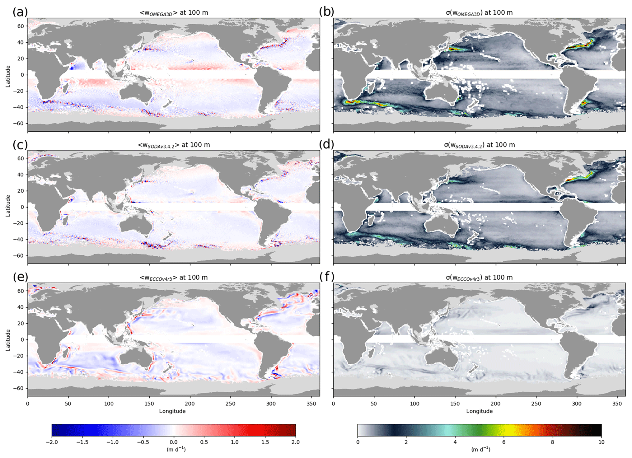
Figure 1Mean vertical velocity at 100 m (a, c, e) and related standard deviation (b, d, f) computed from OMEGA3D (a, b), SODAv3.4.2 (c, d) and ECCOv4r3 (e, f) data on the OMEGA3D domain over their 23-year overlapping period. Areas shallower than 100 m or contaminated at least once by sea ice within the averaging period are masked in light grey.
Specifically, mean vertical velocity patterns at 100 m depth and associated variability (standard deviation) are computed here from OMEGA3D, SODAv3.4.2 and ECCOv4r3 over their 23-year overlapping period (1993–2015), focusing on the domain covered by the OMEGA3D product and thus excluding the 5∘ N–5∘ S band and coastal areas. The large-scale patterns and range of values found in the averaged velocities are quite similar among the three reconstructions (Fig. 1). Maximum absolute mean values reach around 2 m d−1, and areas dominated by large-scale, wind-driven upwelling at high latitudes and by downwelling at mid-latitudes are consistently identified in the three products, with values rarely exceeding 0.5 m d−1. In the intertropical band, OMEGA3D vertical velocities display slightly higher values than the other two reconstructions (especially in the central Pacific). More substantial differences are found along the major western boundary current systems and along the Antarctic Circumpolar Current, where the different nominal resolution and the different dynamical representation of mesoscale features in the three systems are reflected in terms of averaged vertical transport. Specifically, even if OMEGA3D and SODAv3.4.2 display very similar patterns, the former displays stronger values in the Agulhas Return Current and along the Gulf Stream meanders as well as around the northern branch of the anticyclonic gyre around the Zapiola Rise, while the latter presents intensified exchanges in the Pacific–Antarctic Ridge and South Indian Ridge areas. The differences between OMEGA3D and SODAv3.4.2 in the Zapiola Anticyclone, an eddy-driven flow controlled by bottom friction, could be associated with the difficulties in accurately representing that circulation in many global reanalyses. As expected, ECCOv4r3 patterns do not resolve any of the alternated upwelling and downwelling patterns found along the main currents' meanders in the two 0.25∘ resolution products, and its representation of mean vertical velocities in all western boundary currents basically consists of uniform upwelling and downwelling associated with the parameterization of baroclinic instabilities along steep isopycnal slopes. OMEGA3D mean vertical velocity patterns look very similar to SODAv3.4.2 in the northern part of the Atlantic Ocean as well, while ECCOv4r3 presents quite different large-scale patterns.
Given its 5 d sampling, SODAv3.4.2 could be expected to reveal a stronger variability than OMEGA3D (7 d sampling), and both are expected to display much higher values than ECCOv4r3 (providing monthly averaged fields). Conversely, though associated patterns display very similar features, the maximum OMEGA3D standard deviation value exceeds SODAv3.4.2 by a factor of ∼ 2. In both cases, intense maxima are associated with the main current systems.
For the sake of a more consistent comparison with ECCOv4r3, OMEGA3D and SODAv3.4.2 vertical velocity standard deviations have also been estimated after low-pass filtering the latter two time series (by a five-point and seven-point moving window, respectively) to only keep frequencies lower than monthly, like those provided by ECCOv4r3 (Fig. 2 should thus be compared to Fig. 1f). Even in that case, the variability observed in ECCOv4r3 is sensibly lower than those retrieved from higher-spatial-resolution products, likely revealing the limits of the mesoscale parameterization used in ECCOv4r3 in terms of vertical exchanges.
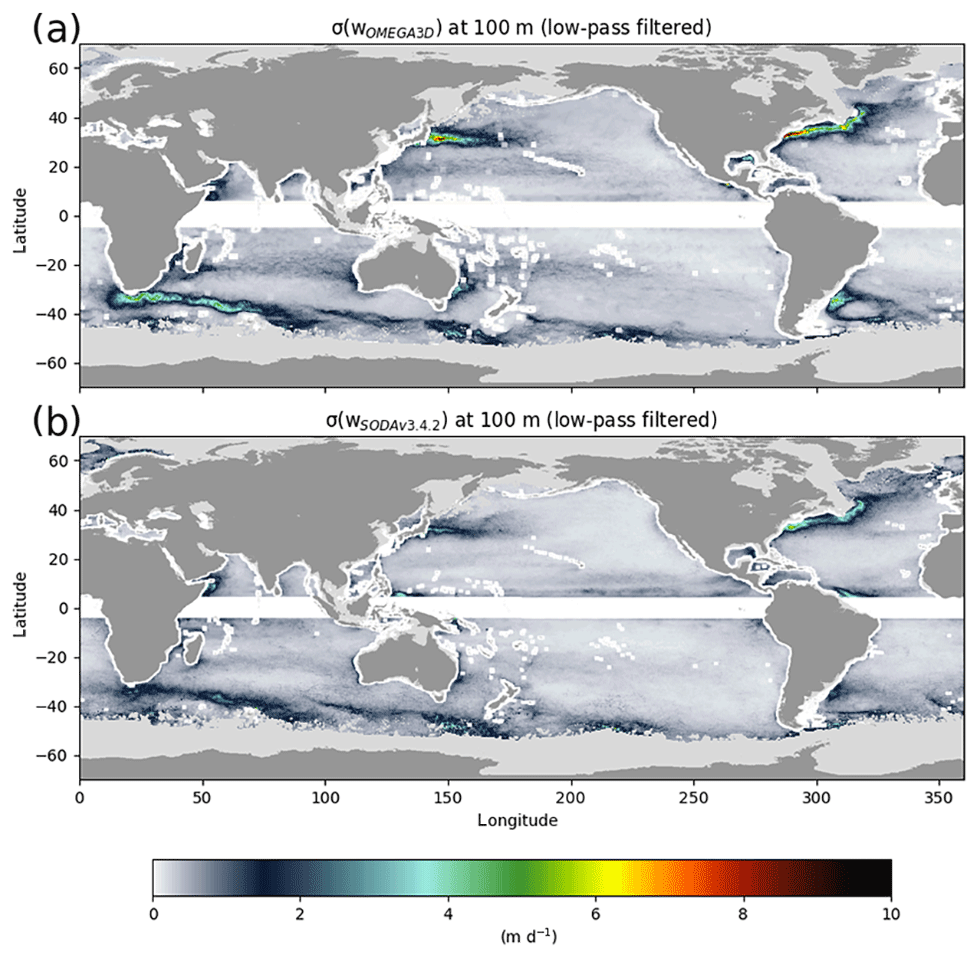
Figure 2Mean monthly vertical velocity patterns and standard deviations computed from OMEGA3D (a) and SODAv3.4.2 (b) after low-pass filtering the time series to remove signals above monthly frequency.
3.4 Horizontal velocity validation vs. independent observations
OMEGA3D horizontal velocity accuracy has been assessed in terms of mean bias and root mean square differences (RMSDs) with respect to space–time-co-located in situ reference observations. Estimated metrics have then been compared to those estimated for geostrophic velocities directly obtained from the Data Unification and Altimeter Combination System (DUACS) altimeter data (when looking at SVP velocities; AVISO+, 2015) or from ARMOR3D (when looking at YOMAHA velocities; Mulet et al., 2012) and also successively compared to similar metrics computed from SODAv3.4.2 and GLORYS12v1 output.
To build our matchup databases, OMEGA3D velocities have been interpolated at the same nominal depth of drifter measurements through a weighted average of the two closest levels.
The first assessment covered surface currents as measured by SVP drifters. As SVP drifters may occasionally lose their drogue, thus failing to correctly represent 15 m depth currents, only drogued SVP drifter data collected within ±12 h from nominal reconstruction dates have been included in our matchup databases (Fig. 3a and b). The same matchup procedure has been applied to DUACS geostrophic velocities, SODAv3.4.2 and GLORYS12v1 (all of which share the same nominal horizontal resolution).

Figure 3Number of matchups within bins between OMEGA3D (a) as well as GLORYS12v1 and SODAv3.4.2 (b) velocities (at 15 m depth) and SVP observations and between OMEGA3D (c) as well as GLORYS12v1 and SODAv3.4.2 (d) velocities (at 1000 m) depth and YOMAHA velocities.
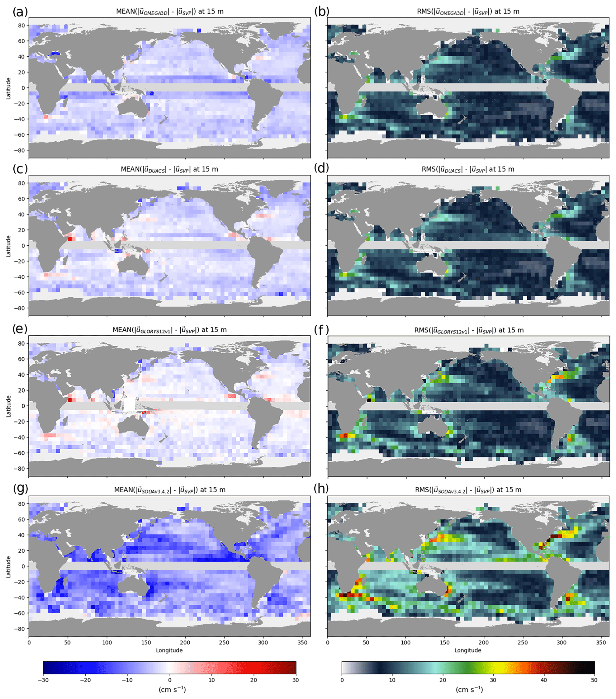
Figure 4Mean and root mean square differences between OMEGA3D (a, b), DUACS (c, d), GLORYS12v1 (e, f) and SODAv3.4.2 (g, h) velocities at 15 m depth and co-located SVP observations.
Mean biases between SVP and OMEGA3D velocities (Fig. 4a) display similar values and patterns to what obtained from altimeter-derived geostrophic velocities (Fig. 4c), with a slight underestimation of the current intensities. OMEGA3D actually appears more biased than DUACS geostrophic velocities close to the tropical band, likely due to the fact that the omega equation is derived from the f plane, and the forcing cannot be correctly estimated there by definition (as accurate horizontal velocities are needed to compute all its terms; see also Sect. 2.3). Overall, their mean biases do not exceed 10 cm s−1. GLORYS12v1 slightly overestimates mean western boundary currents, though it displays very small biases elsewhere (Fig. 4e). Conversely, mean differences between SODAv3.4.2 at 15 m depth and SVP velocities (Fig. 4g) reveal a more significant underestimation of surface currents, with biases reaching up to 20 cm s−1 over wide portions of the domain. Similarly, OMEGA3D and DUACS RMSD values (Fig. 6b and d) present very minor differences, while GLORYS12v1 presents significantly higher differences (by a factor of ∼ 2) along all major currents (Fig. 4f). Even stronger discrepancies affect SODAv3.4.2 estimates, displaying RMSD values up to ∼ 4 times higher than OMEGA3D and DUACS along all major current systems (Fig. 4h). It must be stressed that altimeter data are not assimilated in SODAv3.4.2, and modelled velocities are thus less constrained by observations.
Directly comparing OMEGA3D and DUACS RMSD demonstrates that quasi-geostrophic velocities also improve with respect to geostrophic velocities (by a few centimetres per second), mainly along the Antarctic Circumpolar Current and in the western boundary currents (Fig. 5a).
The second assessment focused on velocities provided by the YOMAHA dataset, which are representative of currents at 1000 m depth. In that case, in order to increase the number of samples, a temporal window of ±1 day has been considered to build the matchup database (Fig. 3c and d).
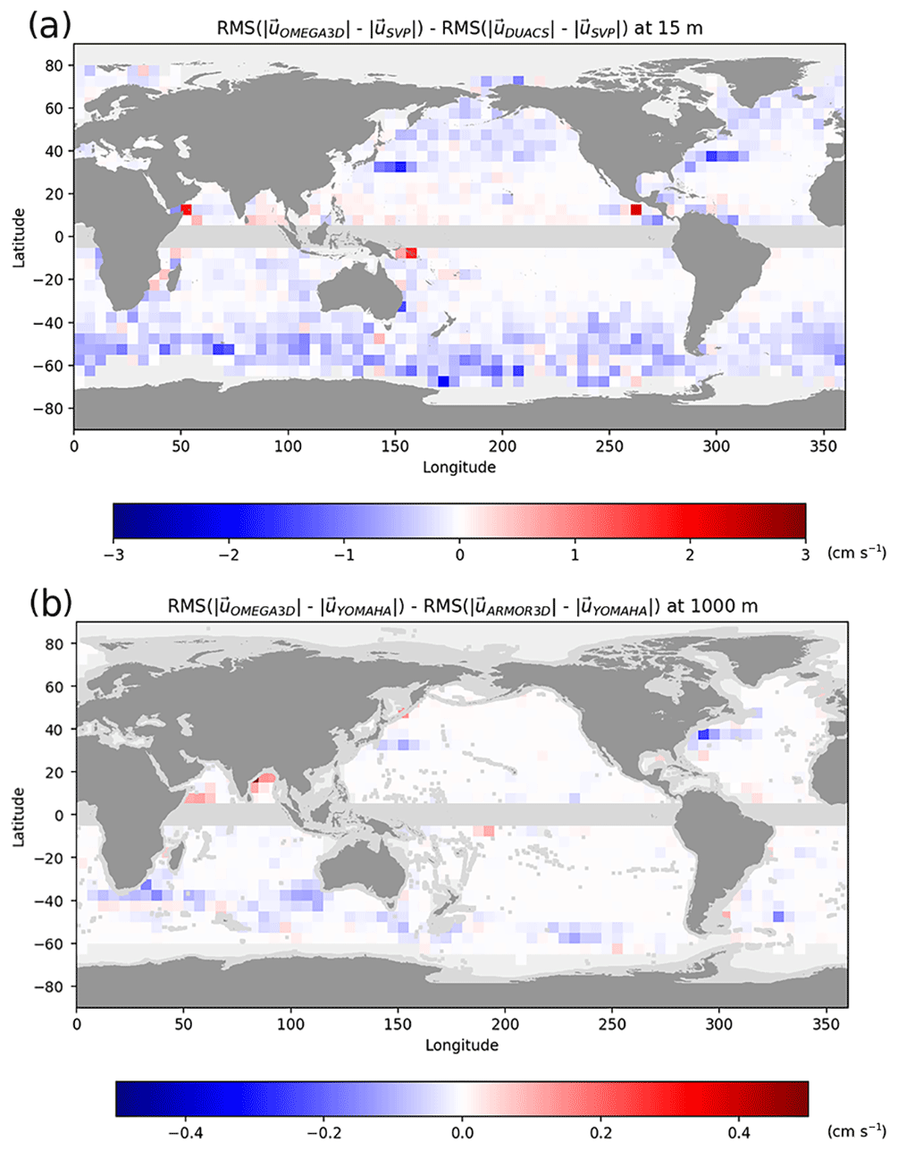
Figure 5RMSD of OMEGA3D quasi-geostrophic and geostrophic horizontal velocities vs. drifters in bins at 15 m (a) and 1000 m (b) depth. Negative values indicate an improvement with respect to geostrophy.
A general overestimation of deep currents is revealed by looking at mean biases with respect to YOMAHA observations. The mean bias attains around 5 cm s−1 in OMEGA3D, ARMOR3D and GLORYS12v1 (Fig. 6a, c, e), while it reaches up to > 15 cm s−1 in SODAv3.4.2 (Fig. 6g). GLORYS12v1 displays more spatially homogeneous values (Fig. 6f), while purely observation-based values tend to overestimate mean western boundary currents but present slightly lower biases elsewhere (especially in the entire Atlantic Ocean). RMSD values computed from OMEGA3D, ARMOR3D and GLORYS12v1 at 1000 m depth (Fig. 6b, d, f) show extremely similar patterns and values. As for surface values, much stronger discrepancies are found between SODAv3.4.2 and YOMAHA estimates, reaching RMSD values up to ∼ 3 times higher along the major current systems (Fig. 6h). Specific comparison of OMEGA3D and ARMOR3D RMSD values also shows that quasi-geostrophic velocities improve with respect to geostrophic velocities in this case, even if by only < 0.5 cm s−1, along the Antarctic Circumpolar Current and in the western boundary currents (Fig. 5b).
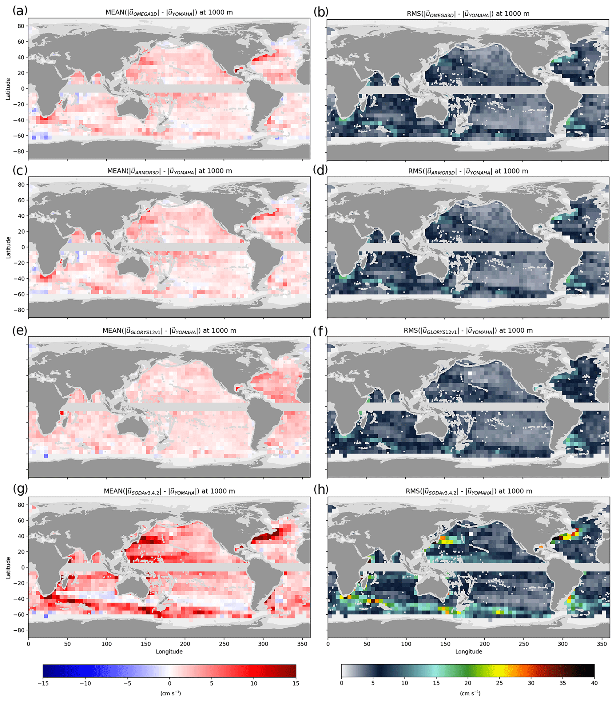
Figure 6Mean and root mean square differences between OMEGA3D (a, b), ARMOR3D (c, d), GLORYS12v1 (e, f) and SODAv3.4.2 (g, h) velocities at 1000 m depth and co-located YOMAHA observations.
The OMEGA3D product is distributed as part of the CMEMS catalogue (https://resources.marine.copernicus.eu/?option=com_csw&task=results?option=com_csw&view=details&product_id=MULTIOBS_GLO_PHY_W_3D_REP_015_007, last access: 23 July 2020, https://doi.org/10.25423/cmcc/multiobs_glo_phy_w_rep_015_007; Buongiorno Nardelli, 2020a). The reduced subset used for validation and review purposes is openly available at https://doi.org/10.5281/zenodo.3696885 (Buongiorno Nardelli, 2020b). Access to the full product is granted after free registration as a user of CMEMS at https://resources.marine.copernicus.eu/?option=com_sla (last access: 23 July 2020). Once registered, users can download the product through a number of different tools and services, including the web portal Subsetter, DirectGetFile (DGF) and FTP. More information can be found at http://marine.copernicus.eu/services-portfolio/technical-faq/ (last access: 23 July 2020).
The basic characteristics of the OMEGA3D product are summarized in Table 1.
The 1993–2018 OMEGA3D time series provides weekly observation-based estimates of the 3D vertical and horizontal ocean currents in the upper 1500 m of the global oceans. The product is obtained by applying a quasi-geostrophic diagnostic model (based on the omega equation) that includes the effect of both geostrophic advection and upper-layer turbulent mixing and delivers, for the first time, estimates of the vertical velocities based on a combination of satellite and in situ observations. The OMEGA3D time series is provided over a 1∕4∘ horizontal grid, and inter-comparison with model reanalyses of comparable length and different space–time resolutions indicates that OMEGA3D resolves the highest amount of vertical velocity variance. Both OMEGA3D and model reanalyses present slightly negative biases with respect to SVP and positive biases with respect to YOMAHA, likely reflecting data representativeness differences and missing processes (or only partially parameterized processes) in models (e.g. sub-mesoscale processes) as well as potentially inaccurate or biased fluxes in the input. OMEGA3D displays the smallest horizontal velocity root mean square differences with respect to independent estimates obtained from drifting-buoy or float displacements (when compared with reanalyses), mostly improving surface current estimates at the mid–high latitudes along the Antarctic Circumpolar Current and in the western boundary currents. Due to the approach followed to retrieve the horizontal ageostrophic components (once the omega equation is solved), the observed improvements (also with respect to simpler geostrophic estimates) mean that estimated vertical velocities should also be deemed reliable.
The model cannot be applied in the equatorial band (where QG approximation fails), and it does not include any parameterization of bottom-boundary-layer mixing. Dirichlet conditions are thus set at the bottom. As a consequence, considering that the domain is also limited to the upper 1500 m, OMEGA3D is not suited for studies of bottom-boundary dynamics or equatorial dynamics. Dirichlet conditions are also applied at coastal boundaries. Even if the effect of lateral-boundary conditions only propagates a few grid points due to the elliptical nature of the omega equation (Buongiorno Nardelli et al., 2001, 2012, 2018a), this also makes the OMEGA3D product unsuitable for studies of coastal dynamics (the product is considered reliable approximately 100 km away from masked coastal areas). As such, OMEGA3D is mostly suited to describe the role and long-term variability of open-ocean, large mesoscale dynamics and air–sea interactions (here parameterized through KPP), for example regarding the vertical exchanges and water mass transformation outside the equatorial band.
The author declares that there is no conflict of interest.
This work has been carried out as part of the Copernicus Marine Environment Monitoring Service Multi Observations Thematic Assembly Center (CMEMS MOB TAC), funded through subcontracting agreement no. CLS-SCO-18-0004 between Consiglio Nazionale delle Ricerche and Collecte Localisation Satellites (CLS), the latter of which is presently leading the CMEMS MOB TAC. The 83-CMEMS-TAC-MOB contract is funded by Mercator Ocean as part of its delegation agreement with the European Union, represented by the European Commission, to set up and manage CMEMS.
This paper was edited by Giuseppe M. R. Manzella and reviewed by Gabriela Pilo and one anonymous referee.
Adcroft, A., Hill, C., Campin, J.-M., Marshall, J., and Heimbach, P.: Overview of the formulation and numerics of the MITgcm, in Proceedings of the ECMWF seminar series on Numerical Methods, Recent developments in numerical methods for atmosphere and ocean modelling, ECMWF, 139–149, 2004.
AVISO+: SSALTO/DUACS User Handbook, CLS-DOS-NT-06-034, Issue 4.4, SALP-MU-P-EA-21065-CLS, 2015.
Baker, A. H., Jessup, E. R., and Manteuffel, T.: A technique for accelerating the convergence of restarted gmres, SIAM J. Matrix Anal. Appl., 26, 962–984, https://doi.org/10.1137/S0895479803422014, 2005.
Balmaseda, M. A., Hernandez, F., Storto, a., Palmer, M. D., Alves, O., Shi, L., Smith, G. C., Toyoda, T., Valdivieso, M., Barnier, B., Behringer, D., Boyer, T., Chang, Y.-S., Chepurin, G. a., Ferry, N., Forget, G., Fujii, Y., Good, S., Guinehut, S., Haines, K., Ishikawa, Y., Keeley, S., Köhl, A., Lee, T., Martin, M. J., Masina, S., Masuda, S., Meyssignac, B., Mogensen, K., Parent, L., Peterson, K. a., Tang, Y. M., Yin, Y., Vernieres, G., Wang, X., Waters, J., Wedd, R., Wang, O., Xue, Y., Chevallier, M., Lemieux, J.-F., Dupont, F., Kuragano, T., Kamachi, M., Awaji, T., Caltabiano, A., Wilmer-Becker, K., and Gaillard, F.: The Ocean Reanalyses Intercomparison Project (ORA-IP), J. Oper. Oceanogr., 8, 80–97, https://doi.org/10.1080/1755876X.2015.1022329, 2015.
Boyer, T. P., Antonov, J. I., Baranova, O. K., Coleman, C., Garcia, H. E., Grodsky, A., Johnson, D. R., Locarnini, R. a, Mishonov, A. V, O'Brien, T. D., Paver, C. R., Reagan, J. R., Seidov, D., Smolyar, I. V, Zweng, M. M., Brien, T. D. O., Paver, C. R., Reagan, J. R., Seidov, D., Smolyar, I. V, Zweng, M. M., and Sullivan, K. D.: WORLD OCEAN DATABASE 2013, NOAA Atlas NESDIS 72, edited by: Levitus, S., NOAA Atlas, 209 pp., https://doi.org/10.7289/V5NZ85MT, 2013.
Buongiorno Nardelli, B.: CNR global observation-based OMEGA3D quasi-geostrophic vertical and horizontal ocean currents (1993–2018) (Version 1), Data set, Copernicus Monitoring Environment Marine Service (CMEMS), available at: https://doi.org/10.25423/cmcc/multiobs_glo_phy_w_rep_015_007, last access: 23rd July 2020a.
Buongiorno Nardelli, B.: CNR global observation-based OMEGA3D quasi-geostrophic vertical and horizontal ocean currents (1993–2018): validation subset (Version V1.0), Data set, Zenodo, https://doi.org/10.5281/zenodo.3696885, 2020b.
Buongiorno Nardelli, B. and Santoleri, R.: Methods for the Reconstruction of Vertical Profiles from Surface Data: Multivariate Analyses, Residual GEM, and Variable Temporal Signals in the North Pacific Ocean, J. Atmos. Ocean. Tech., 22, 1762–1781, https://doi.org/10.1175/JTECH1792.1, 2005.
Buongiorno Nardelli, B., Sparnocchia, S., and Santoleri, R.: Small mesoscale features at a meandering upper-ocean front in the Western Ionian Sea (Mediterranean Sea): Vertical motion and potential vorticity analysis, J. Phys. Oceanogr., 31, 2227–2250, https://doi.org/10.1175/1520-0485(2001)031<2227:SMFAAM>2.0.CO;2, 2001.
Buongiorno Nardelli, B., Guinehut, S., Pascual, A., Drillet, Y., Ruiz, S., and Mulet, S.: Towards high resolution mapping of 3-D mesoscale dynamics from observations, Ocean Sci., 8, 885–901, https://doi.org/10.5194/os-8-885-2012, 2012.
Buongiorno Nardelli, B., Mulet, S., and Iudicone, D.: Three-Dimensional Ageostrophic Motion and Water Mass Subduction in the Southern Ocean, J. Geophys. Res.-Ocean., 123, 1533–1562, https://doi.org/10.1002/2017JC013316, 2018a.
Buongiorno Nardelli, B., Mulet, S., and Iudicone, D.: Three dimensional ageostrophic motion and water mass subduction in the Southern Ocean, J. Geophys. Res.-Ocean., 123, 1533–1562, 2018b.
Cabanes, C., Grouazel, A., von Schuckmann, K., Hamon, M., Turpin, V., Coatanoan, C., Paris, F., Guinehut, S., Boone, C., Ferry, N., de Boyer Montégut, C., Carval, T., Reverdin, G., Pouliquen, S., and Le Traon, P.-Y.: The CORA dataset: validation and diagnostics of in-situ ocean temperature and salinity measurements, Ocean Sci., 9, 1–18, https://doi.org/10.5194/os-9-1-2013, 2013.
Carrassi, A., Bocquet, M., Bertino, L., and Evensen, G.: Data assimilation in the geosciences: An overview of methods, issues, and perspectives, WIRES Clim. Chang., 9, 1–50, https://doi.org/10.1002/wcc.535, 2018.
Carton, J. A., Chepurin, G. A., and Chen, L.: SODA3: A New Ocean Climate Reanalysis, J. Clim., 31, 6967–6983, https://doi.org/10.1175/jcli-d-18-0149.1, 2018.
Danabasoglu, G., McWilliams, J. C., and Gent, P. R.: The role of mesoscale tracer transports in the global ocean circulation, Science, 264, 1123–1126, https://doi.org/10.1126/science.264.5162.1123, 1994.
Dee, D. P., Uppala, S. M., Simmons, A. J., Berrisford, P., Poli, P., Kobayashi, S., Andrae, U., Balmaseda, M. A., Balsamo, G., Bauer, P., Bechtold, P., Beljaars, A. C. M., van de Berg, I., Biblot, J., Bormann, N., Delsol, C., Dragani, R., Fuentes, M., Greer, A. J., Haimberger, L., Healy, S. B., Hersbach, H., Holm, E. V., Isaksen, L., Kallberg, P., Kohler, M., Matricardi, M., McNally, A. P., Mong-Sanz, B. M., Morcette, J.-J., Park, B.-K., Peubey, C., de Rosnay, P., Tavolato, C., Thepaut, J. N., and Vitart, F.: The ERA-Interim reanalysis: Configuration and performance of the data assimilation system, Q. J. Roy. Meteorol. Soc., 137, 553–597, https://doi.org/10.1002/qj.828, 2011.
Delworth, T. L., Rosati, A., Anderson, W., Adcroft, A. J., Balaji, V., Benson, R., Dixon, K., Griffies, S. M., Lee, H. C., Pacanowski, R. C., Vecchi, G. A., Wittenberg, A. T., Zeng, F., and Zhang, R.: Simulated climate and climate change in the GFDL CM2.5 high-resolution coupled climate model, J. Clim., 25, 2755–2781, https://doi.org/10.1175/JCLI-D-11-00316.1, 2012.
Drévillon, M., Régnier, C., Lellouche, J.-M., Garric, G., Bricaud, C., and Hernandez, O.: CMEMS Quality Information Document for Global Ocean Reanalysis Products, GLOBAL-REANALYSIS-PHY-001-030, CMEMS-GLO-QUID-001-030, 2018.
Droghei, R., Buongiorno Nardelli, B., and Santoleri, R.: A New Global Sea Surface Salinity and Density Dataset From Multivariate Observations (1993–2016), Front. Mar. Sci., 5, 1–13, https://doi.org/10.3389/fmars.2018.00084, 2018.
Forget, G., Campin, J.-M., Heimbach, P., Hill, C. N., Ponte, R. M., and Wunsch, C.: ECCO version 4: an integrated framework for non-linear inverse modeling and global ocean state estimation, Geosci. Model Dev., 8, 3071–3104, https://doi.org/10.5194/gmd-8-3071-2015, 2015.
Fukumori, I., Wang, O., Fenty, I., Forget, G., Heimbach, P., and Ponte, R. M.: ECCO Version 4 Release 3, Dspace.Mit.Edu, http://hdl.handle.net/1721.1/110380 (last access: 23 July 2020), 2017.
Fukumori, I., Heimbach, P., Ponte, R. M., and Wunsch, C.: A dynamically consistent, multivariable ocean climatology, B. Am. Meteorol. Soc., 99, 2107–2127, https://doi.org/10.1175/BAMS-D-17-0213.1, 2018.
Gent, P. R. and Mcwilliams, J. C.: Isopycnal Mixing in Ocean Circulation Models, J. Phys. Oceanogr., 20, 150–155, https://doi.org/10.1175/1520-0485(1990)020<0150:IMIOCM>2.0.CO;2, 1990.
Giordani, H., Prieur, L., and Caniaux, G.: Advanced insights into sources of vertical velocity in the ocean, Ocean Dynam., 56, 513–524, https://doi.org/10.1007/s10236-005-0050-1, 2006.
Guinehut, S., Dhomps, A.-L., Larnicol, G., and Le Traon, P.-Y.: High resolution 3-D temperature and salinity fields derived from in situ and satellite observations, Ocean Sci., 8, 845–857, https://doi.org/10.5194/os-8-845-2012, 2012.
Kalnay de Rivas, E.: On the use of nonuniform grids in finite-difference equations, J. Comput. Phys., 10, 202–210, 1972.
Lebedev, K. V, Yoshinari, H., Maximenko, N. A., and Hacker, P. W.: Velocity data assessed from trajectories of Argo floats at parking level and at the sea surface, IPRC Tech. Note, 4, 20 pp., 2007.
Liang, X., Spall, M., and Wunsch, C.: Global Ocean Vertical Velocity From a Dynamically Consistent Ocean State Estimate, J. Geophys. Res. Ocean., 122, 8208–8224, https://doi.org/10.1002/2017JC012985, 2017.
Lopez-Radcenco, M., Pascual, A., Gomez-Navarro, L., Aissa-El-Bey, A., and Fablet, R.: Analog data assimilation for along-track nadiR and SWOT altimetry data in the western Mediterranean Sea, Int. Geosci. Remote Sens. Symp., Valencia, Spain, 22–27 July 2018, 7684–7687, https://doi.org/10.1109/IGARSS.2018.8519089, 2018.
Lumpkin, R., Grodsky, S. A., Centurioni, L., Rio, M. H., Carton, J. A., and Lee, D.: Removing spurious low-frequency variability in drifter velocities, J. Atmos. Ocean. Tech., 30, 353–360, https://doi.org/10.1175/JTECH-D-12-00139.1, 2013.
Lumpkin, R., Özgökmen, T., and Centurioni, L.: Advances in the Application of Surface Drifters, Ann. Rev. Mar. Sci., 9, 59–81, https://doi.org/10.1146/annurev-marine-010816-060641, 2017.
Madec, G. and the NEMO team: NEMO ocean engine, Zenodo, https://doi.org/10.5281/zenodo.3248739, 2016.
Moore, A. M., Martin, M. J., Akella, S., Arango, H. G., Balmaseda, M., Bertino, L., Ciavatta, S., Cornuelle, B., Cummings, J., Frolov, S., Lermusiaux, P., Oddo, P., Oke, P. R., Storto, A., Teruzzi, A., Vidard, A., and Weaver, A. T.: Synthesis of Ocean Observations Using Data Assimilation for Operational, Real-Time and Reanalysis Systems: A More Complete Picture of the State of the Ocean, Front. Mar. Sci., 6, 1–6, https://doi.org/10.3389/fmars.2019.00090, 2019.
Mulet, S., Rio, M.-H., Mignot, A., Guinehut, S., and Morrow, R.: A new estimate of the global 3D geostrophic ocean circulation based on satellite data and in-situ measurements, Deep-Sea Res. Pt. II, 77–80, 70–81, https://doi.org/10.1016/j.dsr2.2012.04.012, 2012.
Reynolds, R. W., Smith, T. M., Liu, C., Chelton, D. B., Casey, K. S., and Schlax, M. G.: Daily High-Resolution-Blended Analyses for Sea Surface Temperature, J. Clim., 20, 5473–5496, https://doi.org/10.1175/2007JCLI1824.1, 2007.
Rio, M.-H., Santoleri, R., and Bourdalle-Badie, R.: Improving the Altimeter-Derived Surface Currents Using High-Resolution Sea Surface Temperature Data?: A Feasability Study Based on Model Outputs, J. Atmos. Ocean. Tech., 33 , 2769–2784, https://doi.org/10.1175/JTECH-D-16-0017.1, 2016.
Smyth, W. D., Skyllingstad, E. D., Crawford, G. B., and Wijesekera, H.: Nonlocal fluxes and Stokes drift effects in the K-profile parameterization, Ocean Dyn., 52, 104–115, https://doi.org/10.1007/s10236-002-0012-9, 2002.
Stammer, D., Balmaseda, M., Heimbach, P., Köhl, A., and Weaver, A.: Ocean Data Assimilation in Support of Climate Applications: Status and Perspectives, Ann. Rev. Mar. Sci., 8, 491–518, https://doi.org/10.1146/annurev-marine-122414-034113, 2016.
Sundqvist, H. and Veronis, G.: A simple finite-difference grid with non-constant intervals, Tellus, 22, 26–31, https://doi.org/10.3402/tellusa.v22i1.10155, 1970.
Ubelmann, C., Klein, P., and Fu, L.-L.: Dynamic Interpolation of Sea Surface Height and Potential Applications for Future High-Resolution Altimetry Mapping, J. Atmos. Ocean. Tech., 32, 177–184, https://doi.org/10.1175/JTECH-D-14-00152.1, 2015.
Ubelmann, C., Cornuelle, B. D., and Fu, L.-L.: Dynamic Mapping of Along-Track Ocean Altimetry?: Method and Performance from Observing System Simulation Experiments, J. Atmos. Ocean. Tech., 33, 1691–1699, https://doi.org/10.1175/JTECH-D-15-0163.1, 2016.
Virtanen, P., Gommers, R., Oliphant, T. E., Haberland, M., Reddy, T., Cournapeau, D., Burovski, E., Peterson, P., Weckesser, W., Bright, J., van der Walt, S. J., Brett, M., Wilson, J., Millman, K. J., Mayorov, N., Nelson, A. R. J., Jones, E., Kern, R., Larson, E., Carey, C., Polat, İ., Feng, Y., Moore, E. W., VanderPlas, J., Laxalde, D., Perktold, J., Cimrman, R., Henriksen, I., Quintero, E. A., Harris, C. R., Archibald, A. M., Ribeiro, A. H., Pedregosa, F., van Mulbregt, P., and SciPy 1.0 Contributors: SciPy 1.0 – Fundamental Algorithms for Scientific Computing in Python, 1–22, arXiv:1907.10121, 2019.
Wunsch, C. and Heimbach, P.: Dynamically and kinematically consistent global ocean circulation and ice state estimates, 2nd edn., Elsevier Ltd., 2013.
Yan, Z., Wu, B., Li, T., Collins, M., Clark, R., Zhou, T., Murphy, J., and Tan, G.: Eastward shift and extension of ENSO-induced tropical precipitation anomalies under global warming, Sci. Adv., 6, eaax4177, https://doi.org/10.1126/sciadv.aax4177, 2020.