the Creative Commons Attribution 4.0 License.
the Creative Commons Attribution 4.0 License.
 | 22 Jul 2020
New ground-based Fourier-transform near-infrared solar absorption measurements of XCO2, XCH4 and XCO at Xianghe, China
Yang Yang
Bavo Langerock
Mahesh Kumar Sha
Christian Hermans
Ting Wang
Denghui Ji
Corinne Vigouroux
Nicolas Kumps
Gengchen Wang
Martine De Mazière
Pucai Wang
The column-averaged dry-air mole fractions of CO2 (XCO2), CH4 (XCH4) and CO (XCO) have been measured with a Bruker IFS 125HR Fourier-transform infrared (FTIR) spectrometer at Xianghe (39.75∘ N, 116.96∘ E, north China) since June 2018. This paper presents the site, the characteristics of the FTIR system and the measurements. The instrumental setup follows the guidelines of the Total Carbon Column Observing Network (TCCON): the near-infrared spectra are recorded by an InGaAs detector together with a CaF2 beam splitter, and the HCl cell measurements are recorded regularly to derive the instrument line shape (ILS) showing that the instrument is correctly aligned. The TCCON standard retrieval code (GGG2014) is applied to retrieve XCO2, XCH4 and XCO. The resulting time series between June 2018 and July 2019 are presented, and the observed seasonal cycles and day-to-day variations in XCO2, XCH4 and XCO at Xianghe are discussed. In addition, the paper shows comparisons between the data products retrieved from the FTIR measurements at Xianghe and co-located Orbiting Carbon Observatory-2 (OCO-2) and Tropospheric Monitoring Instrument (TROPOMI) satellite observations. The comparison results appear consistent with validation results obtained at TCCON sites for XCO2 and XCH4, while for XCO they highlight the occurrence of frequent high-pollution events. As Xianghe lies in a polluted area in north China where there are currently no TCCON sites, this site can fill the TCCON gap in this region and expand the global coverage of the TCCON measurements. The Xianghe FTIR XCO2, XCH4 and XCO data can be obtained at https://doi.org/10.18758/71021049 (Yang et al., 2019).
- Article
(6333 KB) - Full-text XML
- BibTeX
- EndNote


The rapid economic growth of China has contributed to 28.5 % of the global total carbon dioxide (CO2) emissions from fossil fuel consumption and cement production (Jackson et al., 2017). China dominates global CO2 fossil emissions with an average increase of 3.8 % yr−1 between 2008 and 2017 (Le Quéré et al., 2018). In addition, 14 % to 22 % of the global anthropogenic methane (CH4) emissions in the 2000s were attributed to China (Kirschke et al., 2013). It is clear that China should play an important role in the reduction of global carbon emission and climate change mitigation. A decreasing linear trend of % yr−1 in carbon monoxide (CO) concentrations from 2005 to 2016 has been observed over East Asia, and 76 % of this decrease is due to the CO emission control in China (Zheng et al., 2018). However, the estimation of Chinese carbon emissions still has large uncertainties, ranging from ±5 % to ±10 % (Gregg et al., 2008; Le Quéré et al., 2018; Andres et al., 2012). A good understanding of carbon emissions requires accurate monitoring of CO2, CH4, CO and other direct and indirect greenhouse gases.
CO2 is the most important anthropogenic greenhouse gas with a radiative forcing of 1.82±0.19 W m−2 in 2013 (IPCC, 2013). The globally averaged surface dry-air mole fraction of CO2 has increased steadily in the atmosphere from the 278 ppm preindustrial level and has reached up to 405.5±0.1 ppm in 2017. The annual increasing rate of CO2 in the atmosphere during the last 10 years is 2.24 ppm yr−1 (WMO, 2018). The enhancement of CO2 is primarily caused by human activities, such as fossil fuel burning and land-use change (Peters et al., 2012). Atmospheric CH4 is the second important anthropogenic greenhouse gas, and its globally averaged surface dry-air mole fraction increased from the preindustrial level of 722 ppb up to 1859±2 ppb in 2017, with an average growth rate of 7 ppb yr−1 during the last decade (WMO, 2018). Although the CH4 abundance is much lower than that of CO2, the comparative impact of CH4 is about 28 times greater than CO2 over a 100-year period. It is reported that the radiative forcing of CH4 has increased to 0.48±0.05 W m−2 in 2013. A total of 50 %–65 % of CH4 is released from human activities such as energy production–consumption, industry, agriculture, biomass burning and waste management activities, and another 40 % is released from natural emissions (IPCC, 2013). Atmospheric CO is an indirect greenhouse gas and is mainly emitted from fossil fuel combustion and biomass burning (Yin et al., 2015).
The Total Carbon Column Observing Network (TCCON) uses ground-based FTIR spectrometers to measure the direct solar radiation in the near-infrared spectral region, from which the total column-averaged dry-air mole fractions of CO2, CH4, N2O, CO, hydrogen fluoride (HF), H2O and semi-heavy water (HDO) are retrieved (Wunch et al., 2011b). Because of their relatively high precision and accuracy, TCCON data are widely used in satellite validations and model comparisons (Zhou et al., 2016; Ostler et al., 2016; Crisp et al., 2017; Borsdorff et al., 2018; Velazco et al., 2019). Today, there are 25 active TCCON sites (https://tccon-wiki.caltech.edu/, last access: 11 July 2020) covering the latitude band from 80∘ N to 45∘ S. Most TCCON sites are in North America, Europe, East Asia (South Korea and Japan) and Oceania. The Hefei station, located in eastern China, is the first Chinese site that will potentially join the TCCON network. In 2016, a FTIR Bruker IFS 125HR instrument was installed at Xianghe (39.75∘ N, 116.96∘ E, 30 m a.s.l.) and started observations following the TCCON settings in June 2018. As there are no TCCON sites in north China, the FTIR instrument at Xianghe aims to fill the gap in the network in this region.
The Japanese Greenhouse gases Observing Satellite (GOSAT) was successfully launched in 2009 by the Japan Aerospace Exploration Agency (JAXA). It is the first spacecraft to measure atmospheric CO2 and CH4 with high-resolution spectra at shortwave infrared (SWIR) wavelengths (Kuze et al., 2009). The Orbiting Carbon Observatory-2 (OCO-2) was launched on 2 July 2014 by the US National Aeronautics and Space Administration (NASA) and is devoted to enhancing our understanding of regional-scale CO2 exchanges between the surface and the atmosphere (Crisp et al., 2004; Eldering et al., 2017; Crisp et al., 2017). The Tropospheric Monitoring Instrument (TROPOMI) was launched by the European Space Agency (ESA) on 13 October 2017 as the single payload of the Sentinel-5 Precursor (S5P) satellite. It aims at providing accurate and timely observations of abundances of atmospheric species, such as CH4 and CO, for air quality and climate change research and services (Borsdorff et al., 2018). However, previous validation work (Wunch et al., 2017; Lambert et al., 2019) based on FTIR measurements has not been carried out in north China due to the absence of TCCON sites in this area; thus it is important to add a Xianghe site for evaluation of satellite products in this area.
In this paper, we describe the ground-based FTIR system at Xianghe, with a focus on the measurements of atmospheric CO2, CH4 and CO (Yang et al., 2019). The column-averaged dry-air mole fractions of these gases are retrieved by the GGG2014 (Wunch et al., 2015) code in the period between 14 June 2018 and 19 July 2019. The paper is structured as follows. Section 2 introduces the Xianghe site and the FTIR system. In Sect. 3, the retrieval and filtering methods are described. The time series of XCO2, XCH4 and XCO are shown and discussed. In the next section, the OCO-2 (XCO2) and TROPOMI (XCH4 and XCO) satellite observations are compared with the FTIR measurements at Xianghe. Finally, conclusions are drawn in Sect. 5.
2.1 Location and experimental setup
The Xianghe site has been operated by the Institute of Atmospheric Physics, Chinese Academy of Sciences since 1974. The site is about 50 km to the east-southeast of Beijing and 70 km to the north-northwest of Tianjin (see Fig. 1b). The Xianghe county acts as an integrated transportation and transfer center in the Beijing–Tianjin–Hebei region, which is one of the most populous and economically dynamic areas in China (Ran et al., 2016). Xianghe has a middle-latitude monsoon climate, with a prevailing southeast wind in summer and a northwest wind in winter (Song et al., 2011). The maximum temperature at the Xianghe site is around 38 ∘C in summer, and the minimum temperature is around −10 ∘C in winter. The raining days occur mainly in summer including some days with extreme precipitation larger than 100 mm d−1.
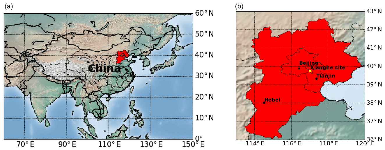
Figure 1Map of China (a); the Beijing–Tianjin–Hebei region is the red shaded area also enlarged in (b). It is one of the most populous and economically dynamic regions in China. The Xianghe site (yellow spot in b) is located in Xianghe County, about 50 km to the east-southeast of Beijing and 70 km to the north-northwest of Tianjin.
The Bruker IFS 125HR instrument was installed in the upper level of a four-story building in June 2016. About 2 years later, in June 2018, a solar tracker was installed on the roof (50 m a.s.l.), to guide the direct solar radiation into the FTIR instrument. The distance between the solar tracker and the entrance window of the FTIR instrument is about 3 m. The solar tracker uses a camera inside the IFS 125HR spectrometer to ensure that the center of the solar disk always focuses on the entrance aperture of the spectrometer, with an active feedback loop. This system is set up following the developments from Neefs et al. (2007) and Gisi et al. (2011). The FTIR instrument operates only under clear-sky daytime conditions. A rain sensor and a solar irradiation (both total and direct) sensor are installed next to the solar tracker, to monitor the weather conditions and to control the opening and closing of the solar tracker hatch. To protect the mirrors (aluminum, coating with MgF2) of the solar tracker, the hatch of the tracker automatically closes under rainy conditions and during nighttime. A heating system is operated in the tracker system to keep the temperature of the rotatory stages and the mirrors close to 15 ∘C in winter. Inside the lab, the air-conditioning keeps the room temperature stabilized around 25 ∘C.
The near-infrared (NIR) spectra are recorded by an indium gallium arsenide (InGaAs) detector, and the middle-infrared (MIR) spectra are recorded by a liquid-nitrogen-cooled indium antimonide (InSb) detector. The entrance window and the beam splitter are made of CaF2. The spectral ranges of the NIR and MIR spectra are 3800–11 000 and 2000–5000 cm−1, respectively. The InSb detector at Xianghe records spectra in the AC mode. The InGaAs detector at Xianghe was operated in the AC mode before 31 May 2019 but since then in the AC + DC mode to be compliant with TCCON standards. The spectrometer settings automatically alternate between NIR and MIR measurements during each clear-sky day. The entrance aperture of the spectrometer in the NIR spectrum was set to 0.5 mm and changed to 0.8 mm after 19 June 2019. There are approximately 70 NIR InGaAs spectra for each clear day. The InGaAs spectra are recorded with a maximum optical path difference (MOPD) of 45 cm, corresponding to a spectral resolution of 0.02 cm−1. Each measurement contains two scans (one forward and one backward), taking about 145 s.
About 50 m southwest of the laboratory building, a weather station is operated on a 110 m tall tower, at 62 m above the ground, measuring pressure, temperature, humidity, wind direction and wind speed. The pressure sensor is located inside the LI-7550 analyzer, which has an accuracy of 1 hPa. On 30 May 2019, a new weather station was installed at the same height as the solar tracker. The distance between the weather station and the solar tracker is about 2 m. The pressure sensor is a PTB210A digital barometer, with an accuracy of 0.25 hPa.
2.2 Instrument line shape
The instrument line shape (ILS) reflects the performance and alignment of the instrument, which might be distorted by the shear or angular misalignment of the instrument or the field of view (FOV) (Schneider et al., 2008). A perfectly aligned interferometer will perfectly center the Haidinger fringes on the field stop at all optical path differences (OPDs). The offset between the moving cube-corner retro-reflector (CCRR) and the fixed CCRR will cause the Haidinger fringes to move away from the center when the mirror moves away from zero optical path difference (ZOPD), and this is called shear misalignment. The angular misalignment is caused when the IR beam is not parallel to the rails. According to the TCCON requirements, modulation efficiency (ME) amplitude changes must be within 5 % at MOPD and phase error (PE) less than 0.02 rad (Wunch et al., 2011b). A sensitivity study performed by Hase et al. (2013) showed that the uncertainty in XCO2 is about 0.035 % (0.14 ppm) for a ME change of 4 %, which is within the 0.8 ppm (solar zenith angle (SZA) less than 80∘) estimated retrieval accuracy of TCCON XCO2.
At Xianghe two HCl cell spectra are recorded every day after sunset, but the tungsten lamp used to measure the HCl cell spectra broke down in February 2019 so that there is no HCl cell measurement after that day. The ME amplitude and PE are retrieved by LINEFIT14.5 using 13 HCl microwindows under non-vacuum status (Hase et al., 1999). The degrees of freedom for signal (DOFS) of apodization and phase are about 4.1 and 4.2, respectively. The ME is derived from the ratio of the misaligned fringe amplitude to the theoretical fringe amplitude. LINEFIT14.5 normalizes ME to be 1.0 at ZOPD. Figure 2 shows the ME and PE along with the OPD, together with the maximum ME loss and maximum PE deviation at Xianghe. The ME has a maximum loss at the MOPD while PE has a maximum deviation at about 20 cm (positive value) or the MOPD (negative value). The mean of the maximum ME loss is 0.022±0.004, and the mean of the maximum absolute PE deviation is 0.014±0.003 rad. Only a few days in September 2018 have a maximum absolute PE slightly larger than 0.02 rad. In general, the alignment of the instrument slightly declines over time, but the ME and PE remain compliant with the TCCON requirements during the whole time period.
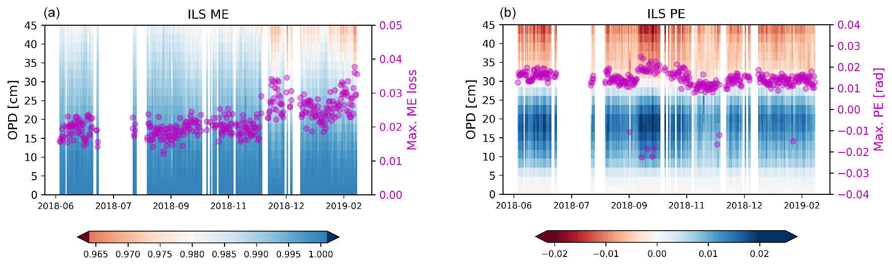
Figure 2The modulation efficiency (ME, a) and phase error (PE, b) along the optical path difference (OPD) at Xianghe. The purple dots are the maximum ME loss (a) and the maximum PE deviation (b).
2.3 Signal-to-noise ratio
The time series of the signal-to-noise ratio (SNR) of the InGaAs spectra at Xianghe is shown in Fig. 3. The SNR (Eq. 1) is calculated as the ratio between the maximum intensity (max(I)) of the spectrum in the spectral range of 3800–11 000 cm−1 and the noise level. The standard deviation of the intensity between 2350 and 2450 cm−1 (SD(noise)) is calculated as the noise level, since no signal is recorded in this window,
There are no measurements between 7 July and 22 August 2018 due to a power cut. The SNR decreases quickly with time because Xianghe is located in a polluted area, causing rapid degradation of the mirrors of the solar tracker (Feist et al., 2016). In order to obtain a high SNR, the mirror of the solar tracker was cleaned on 14 November 2018 (first yellow line in Fig. 3), with the SNR increasing from 300 to 500. However, the SNR decreased back to the level of 300 about 3 weeks later, probably because of the increased level of air pollution and relatively lower solar irradiation in winter. The polluted mirror of the solar tracker was replaced with a new one on 1 February 2019 (second yellow line in Fig. 3), enhancing the SNR from about 300 to 450. With the DC signal recording (first red line in Fig. 3), between 31 May and 19 June 2019 the SNR dropped quickly below 200. Therefore, the aperture size was increased from 0.5 to 0.8 mm on 19 June 2019 (second red line in Fig. 3), and the mirror was cleaned again on 25 June 2019 (third yellow line in Fig. 3), making the SNR rise again above the level of 300.
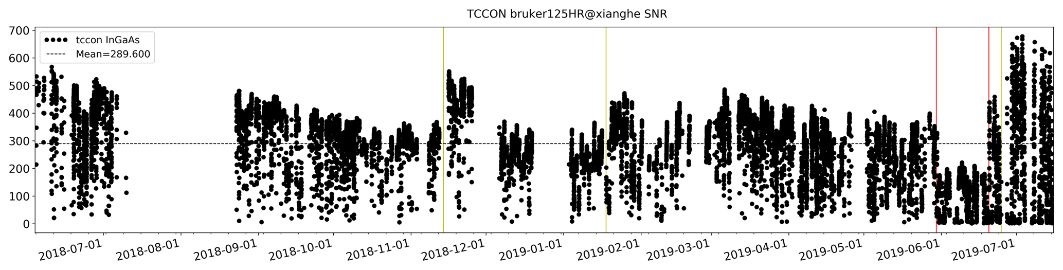
Figure 3Time series of the signal-to-noise ratio (SNR) of the InGaAs spectra from the FTIR instrument in Xianghe. The yellow lines indicate solar tracker maintenances: cleaning of the mirrors on 14 November 2018 and 25 June 2019 and replacement of the degraded mirror on 1 February 2019. The first red line indicates the day when we add DC signal recording (31 May 2019), and the second red line indicates the day when the aperture was increased from 0.5 to 0.8 mm (19 June 2019).
3.1 Retrieval methodology
The nonlinear least-squares fitting code GGG2014 (Wunch et al., 2015) is used to retrieve XCO2, XCH4, XCO and some other gases from the NIR solar absorption spectra at Xianghe,
where TCa and TCr are the a priori and retrieved total columns, A is the column averaging kernel, xt and xa are true and a priori partial column profiles, and ε is the uncertainty. In the forward model, there are 70 equidistant 1 km thick layers from the mean sea level up to 70 km altitude. The a priori profiles of gases are generated by an empirical model based on surface in situ, Atmospheric Chemistry Experiment Fourier Transform Spectrometer (ACE-FTS) and the Jet Propulsion Laboratory MkIV (Mark IV) interferometer measurements. The interannual trends and seasonal variations in the species are taken into account, and the a priori profiles are adjusted based on the local tropopause pressure at local noon (Toon and Wunch, 2015). The temperature, pressure and water vapor profiles are taken from the National Centers for Environmental Prediction (NCEP) reanalysis data (Kalnay et al., 1996). The surface pressure, temperature and water vapor are from the local weather station.
The column averaging kernel represents the vertical sensitivity of the retrieved total column to the true partial column profile. The typical averaging kernels of XCO2, XCH4 and XCO are shown in Fig. 4 of Wunch et al. (2011a). In general, the retrieved CO2 and CH4 total columns have good sensitivity in the troposphere and the stratosphere. The retrieved CO column underestimates a deviation from the a priori partial column in the troposphere but overestimates a deviation from the a priori partial column in the stratosphere.
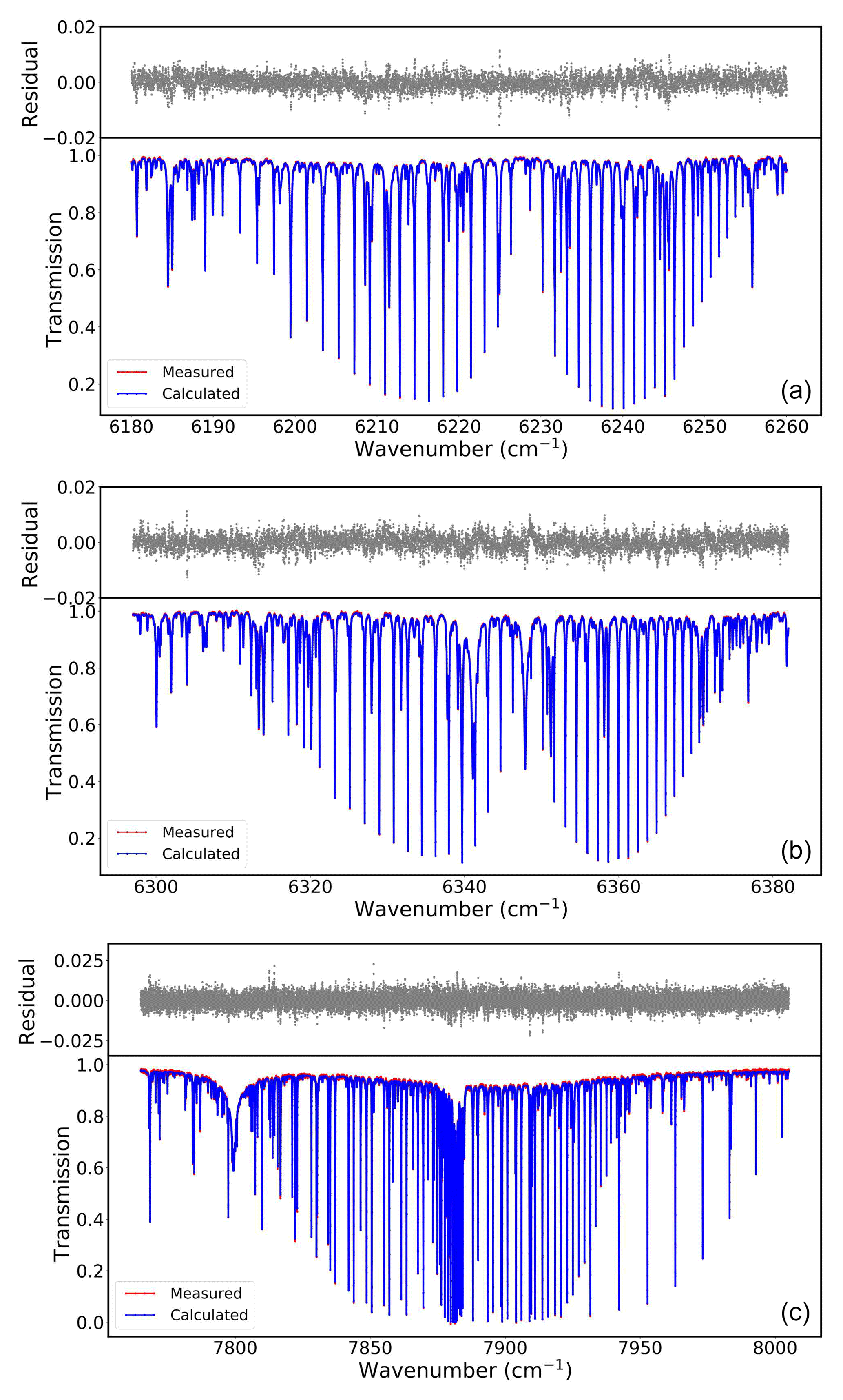
Figure 4Measured and calculated spectrum of CO2 in a spectral window of 6180–6260 cm−1 (a), CO2 in a spectral window of 6297–6382 cm−1 (b) and O2 in spectral window of 7765–8005 cm−1 (c).
The retrieval windows of CO2, CH4, CO and O2 are listed in Table 1 in Wunch et al. (2010). As an example, Fig. 4 shows the residuals of the spectral fitting for CO2 and O2 for one NIR spectrum at a SZA of 22.9∘ at Xianghe. The root mean square of the residuals for CO2 in the spectral window 6180–6260 cm −1, CO2 in the window 6297–6382 cm−1 and O2 in the window 7765–8005 cm−1 are 0.24 %, 0.25 % and 0.37 %, respectively, which compare well to the results in Toon et al. (2009).
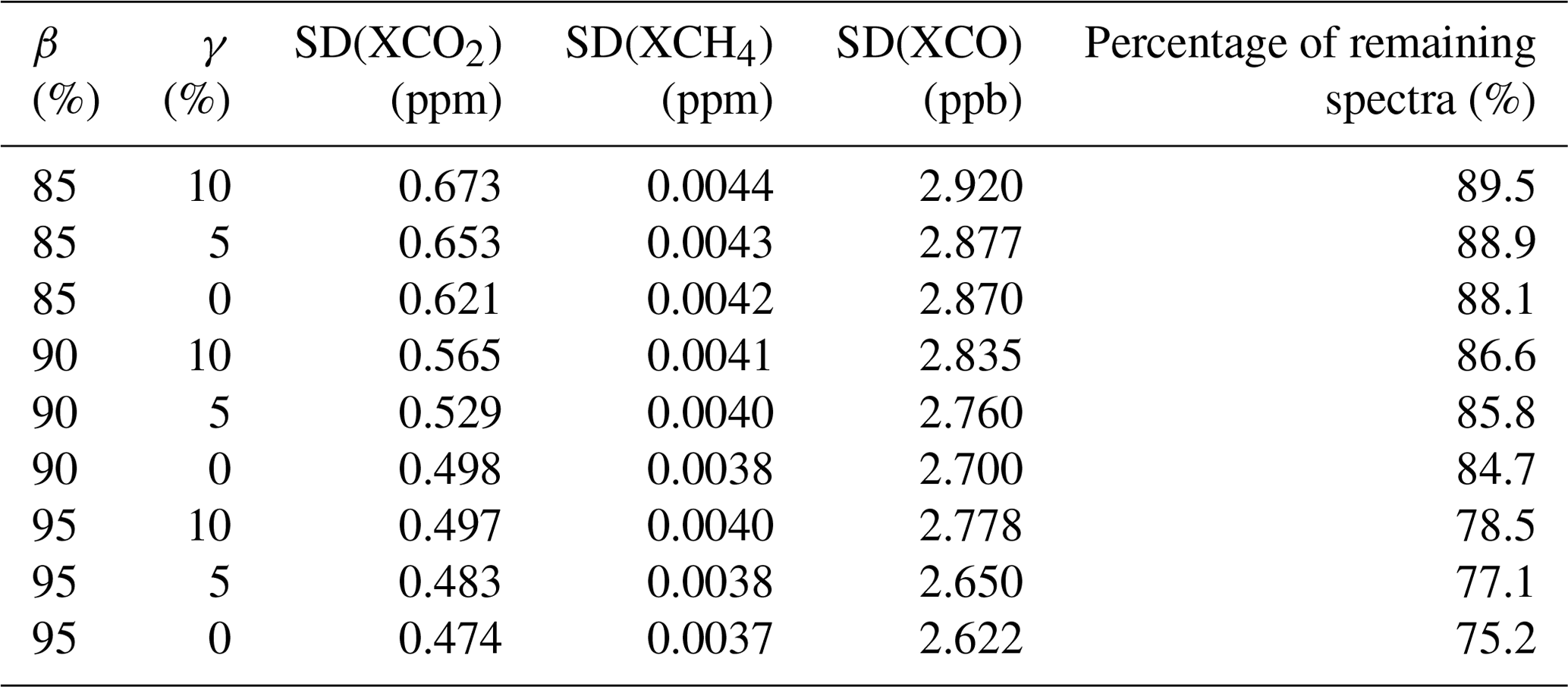
Table 1The SD of XCO2, XCH4 and XCO of the remaining data after each solar intensity (SI) filtering for each day and the percentage of the remaining number of spectra from 14 June to 31 December 2018. Only measurements recorded within the ±1 h window around local noon are considered.
The spectroscopy is the atmospheric (ATM) line list (Toon, 2017). The total column-averaged dry-air mole fraction of gas (Xgas) is then derived from the ratio between the retrieved total column of the target species and the retrieved total column of O2 ,
Using the ratio between the target species and O2 reduces the uncertainties common to both gases, e.g., the surface pressure, water vapor, solar tracker pointing and zero level offsets. In addition, a post-processing of the results is done: (1) the air mass dependence of the retrieval results which is known to be an artifact caused by spectroscopic uncertainties is reduced by applying an empirical air-mass-dependent correction, and (2) a scaling factor for each gas is applied to calibrate the TCCON measurements to the WMO scale (Wunch et al., 2010, 2015).
3.2 Data quality control
As the recording time for one InGaAs spectrum takes about 145 s, the stability of the incoming solar intensity during this period is important for the quality of the spectrum (Beer, 1992). If there are clouds or heavy aerosols in the light path between the FTIR instrument and the sun during the spectrum recording, the fractional line depth in FTIR spectra will be distorted (Ridder et al., 2011; Keppel-Aleks et al., 2011). In order to select the good-quality spectra, we filter out the spectra with a SNR less than 200, apart from the period between 31 May and 19 June 2019 where we filter out the spectra with a SNR less than 100.
The DC correction can be used to remove the solar irradiation variation in each spectrum (Keppel-Aleks et al., 2007). To filter out spectra affected by the occurrence of clouds or high aerosol load before 31 May 2019 (in AC recording mode), we use the variations in the direct solar irradiation observed from the solar irradiation detector installed close to the solar tracker system (see Sect. 2.1). The solar direct irradiation is recorded every 3 s, providing us with about 25 measurement points per forward or backward scan. If the sky is clear, the direct solar irradiation should remain relatively stable. We classify measurement points during the scan as problematic if the solar intensity is lower than a certain percentage threshold β of the maximum intensity. A spectrum is selected as a good one if the number of problematic measurement points is smaller than or equal to a certain percentage threshold γ of the total number of measurement points during the measurement. We test the filtering method with γ values of 0 %, 5 % and 10 % and β values of 85 %, 90 % and 95 % on all InGaAs spectra from 14 June to 31 December 2018. To estimate the precision of the retrievals at Xianghe, we calculate the standard deviations (SD) of the retrievals in a time window of ±1 h around local noon. By using the 2 h window, the potential influences can be reduced, such as a diurnal cycle, the influence of local sources in such a heavily urbanized area and a residual air mass dependence of the retrievals as pressure broadening is not accounted for in the GGG2014 spectroscopy. We select all the days when at least five measurements are available. The results are shown in Table 1. The SDs of XCO2, XCH4 and XCO decrease with increasing β or decreasing γ thresholds. According to Pollard et al. (2017), the precision target for TCCON is 0.1 % (∼0.4 ppm) for XCO2 to meet the model requirements (Olsen and Randerson, 2004). However, the precision of the TCCON XCO2 is estimated to be 0.2 % (∼0.8 ppm) based on the perturbation of the GGG2014 inputs (Wunch et al., 2015). In order to reduce the variation in the measurements and to keep as many useful measurements as possible, we choose β=90 % and γ=0 % as the criteria for the solar intensity (SI) filtering. The mean SDs of XCO2, XCH4 and XCO are 0.498 ppm, 0.0038 ppm and 2.700 ppb, respectively, and there are 84.7 % spectra remaining. Note that the mean SD of XCO2 is 0.12 %, which is slightly worse than the target of the TCCON XCO2 precision of 0.1 %, but it is better than the estimated uncertainty of 0.2 %. To evaluate the precision of the retrievals at Xianghe, we compare the SD of XCO2 measurements at Xianghe with several TCCON sites with similar latitude (Lamont, Karlsruhe, Pasadena, Rikubetsu, Tsukuba, Saga, Orléans and Anmeyondo), and the SD of XCO2 at Xianghe is comparable with these sites.
The 110 m height meteorology tower is collinear with the solar irradiation sensor and the sun tracker. It generates a shadow on the mirror of the tracker system, affecting the spectra in the afternoon. The duration of the shadow is about 8–15 min, corresponding to about two to three InGaAs measurements. The shadow occurs at around 06:30 UTC (14:30 LTC) in summer and around 09:30 UTC (16:30 LTC) in winter. Figure 5 shows the direct solar intensity from 1 to 3 October 2018, with a zoom in over the time period between 06:36 and 07:02 (UTC) on 2 October 2018 when the tower shadow is observed by the FTIR instrument (see the inside camera image). The XCO2 retrievals are strongly affected by the tower shadow. However, Fig. 5 shows that the spectra polluted by the tower shadow can be filtered out by the combination of SNR filtering and SI filtering with β=90 % and γ=0 %.
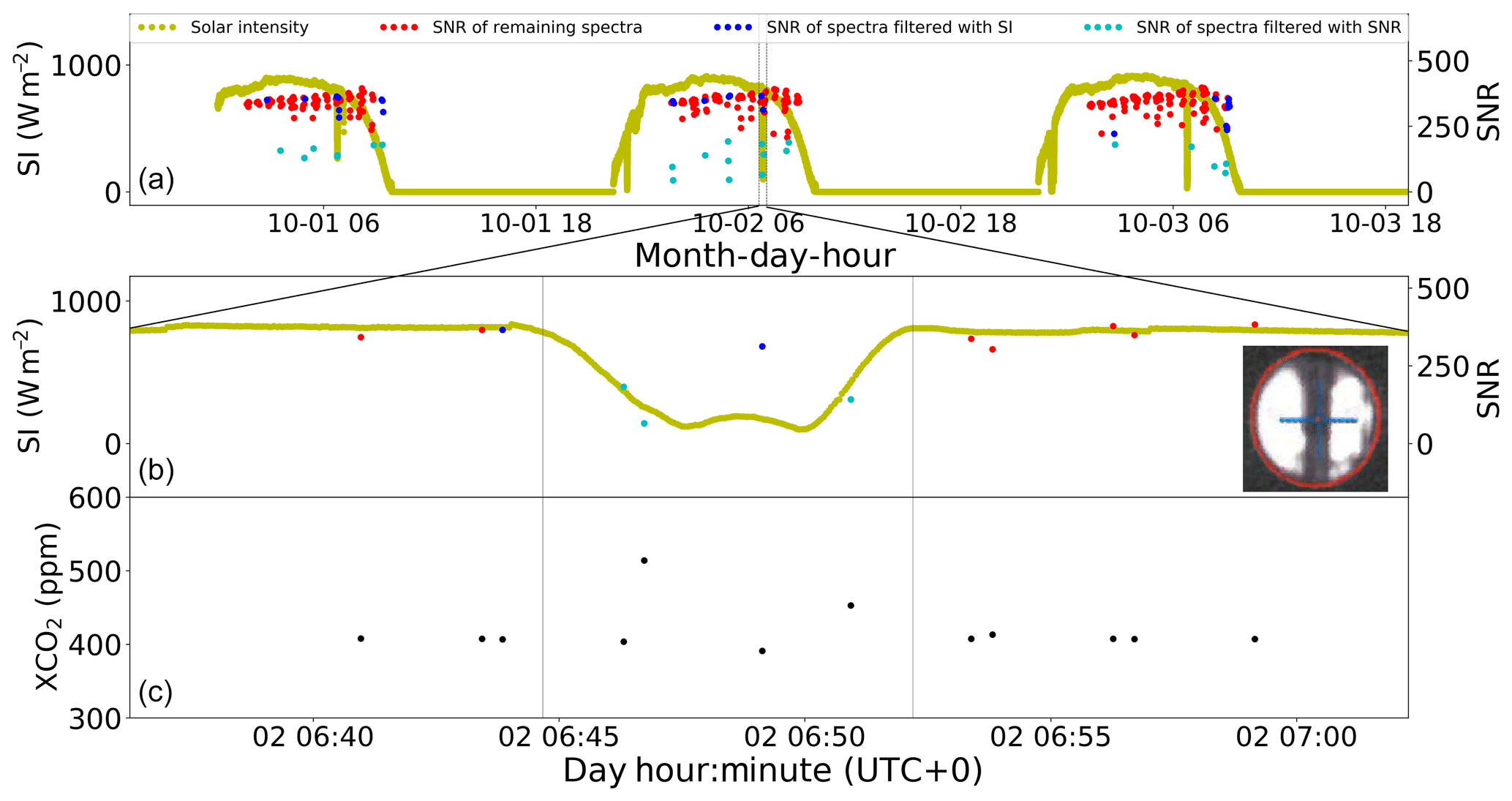
Figure 5The direct solar intensity from 1 to 3 October 2018, with a zoom of the time period between 06:36 and 07:02 (UTC) on 2 October 2018 when the tower shadow is observed by the FTIR instrument (see the inside camera image, b). The blue dots (a) denote the SNR of spectra filtered with solar intensity (SI), the cyan dots denote the SNR of spectra filtered with SNR and the red dots denote the SNR of spectra after both filters. The XCO2 retrievals during the time with the shadow are displayed in (c).
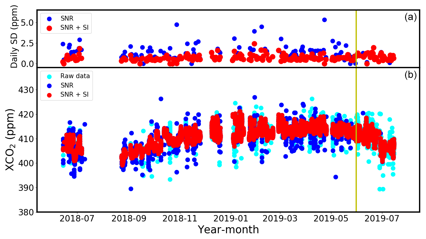
Figure 6Time series of XCO2 from 14 June 2018 to 19 July 2019 before and after spectra selection. The cyan dots denote all the raw data, the blue dots in (b) are the retrieved XCO2 after SNR filtering and the red dots are the retrieved XCO2 after SNR + SI filtering. In (a), the blue dots denote the daily standard deviation of XCO2 only with SNR filtering while the red ones denote those with SNR + SI filtering. The yellow line denotes the day (31 May 2019) when we added the DC signal recording.
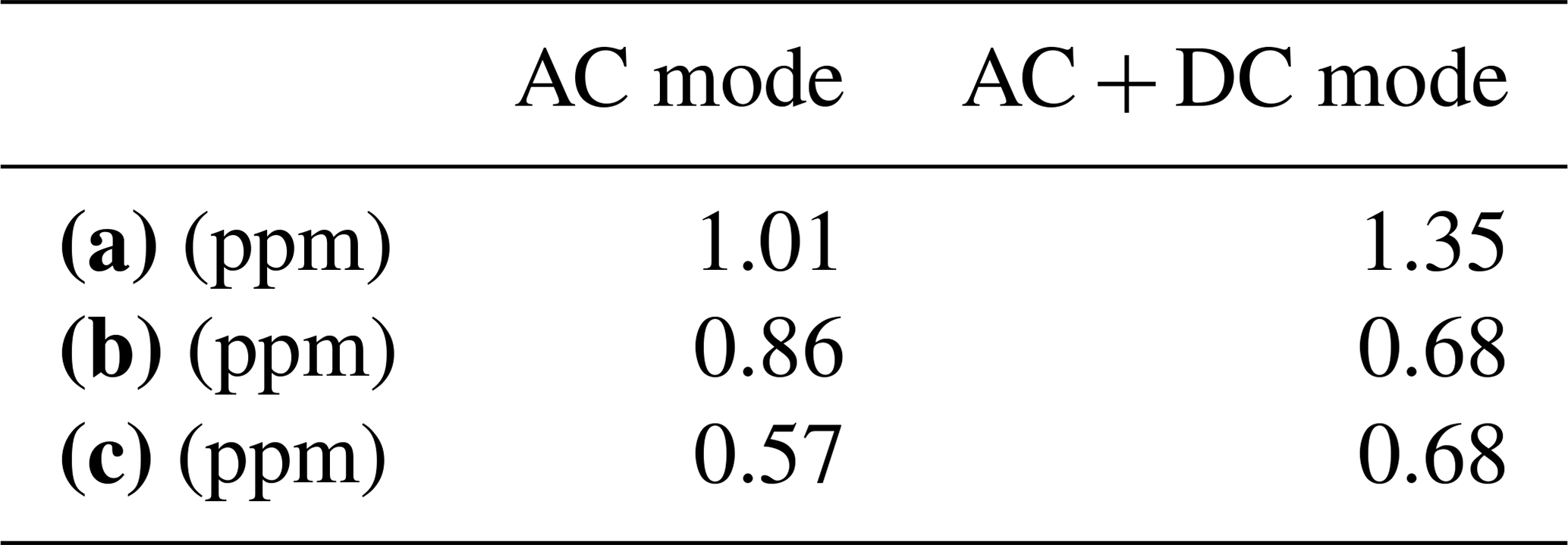
Figure 6 shows the time series of XCO2 with and without filtering between 14 June 2018 and 19 July 2019. Based on the measurements with the recorded time within the ±1 h window around local noon, Table 2 shows that SNR filtering apparently reduces the average daily SDs both before (from 1.01 to 0.86 ppm) and after (from 1.35 to 0.68 ppm) DC signal recording. It is clear that before DC recording, many XCO2 outliers are removed by the SI filtering, with the average daily SD of XCO2 decreasing from 0.86 ppm to 0.57 ppm. However, the SI filtering does not change the SD of XCO2 (0.68 ppm) from the DC to AC + DC period due to the fact that the DC correction already corrects the solar variation. Therefore, for the period with AC + DC mode, only the SNR filtering is applied.
Table 2Average XCO2 daily SD after (a) no filtering, (b) SNR filtering, and (c) both SNR filtering and SI filtering during the AC mode and AC + DC mode periods. Only those measurements recorded within the ±1 h window around local noon are considered.
Poor instrument alignment, spectral ghost, error in the time assigned to the spectrum or faulty pressure sensor may cause a dramatic jump in Xair (Washenfelder et al., 2006; Wunch et al., 2011a). The retrieved Xair values (after filtering) are shown in Fig. 7 to confirm the good quality of the retrievals. Xair is defined as
where mdry,air and are the molecular mass of dry air and water vapor, and g is the column-averaged gravitational acceleration. Ps is the surface pressure, and TCdry,air, TC and TC are total columns of dry air, O2 and H2O, respectively. The Xair is around 0.98 due to a ∼2.0 % bias in the O2 spectroscopy (Kivi and Heikkinen, 2016). Figure 7 shows that the Xair values at Xianghe all pass TCCON standard quality check (between 0.96 and 1.04) and are stable over time with a mean value of 0.982 and a SD of 0.003.
3.3 Retrieval results and discussions
The time series of XCO2, XCH4 and XCO after both SNR and SI filtering from June 2018 to July 2019 are shown in Fig. 8. The monthly means of XCO2, XCH4 and XCO at Xianghe, Pasadena (34.1∘ N) (Wennberg et al., 2014), Lamont (36.6∘ N) (Wennberg et al., 2016) and Karlsruhe (49.1∘ N) (Hase et al., 2014) from June 2018 are also displayed in Fig. 9. Based on these measurements, the seasonal variations and day-to-day variations in XCO2, XCH4 and XCO are assessed. XCO2 is low in summer and high in winter and spring at Xianghe, with a maximum monthly mean of 414.37±0.97 ppm in April 2019 and minimum monthly mean of 401.95±1.43 ppm in August 2018. This seasonal behavior is similar to that at Pasadena, Lamont and Karlsruhe, which are located in the northern midlatitude zone. The peak-to-peak amplitude of the seasonal variation in XCO2 is 12.42 ppm, which is larger than 7.45 ppm at Pasadena, 7.78 ppm at Lamont and 7.98 ppm at Karlsruhe. XCH4 is low in spring and high in autumn and summer, with a maximum monthly mean of 1.898±0.019 ppm in August 2018 and a minimum monthly mean of 1.858±0.014 ppm in March 2019. It is found that the seasonal cycle of the XCH4 at Xianghe is very different with other sites at a similar latitude, as the observations at the other three stations show low values in summer and high values in autumn and winter. The peak-to-peak amplitude of the XCH4 seasonal variation is about 0.040 ppm at Xianghe, which is also larger than 0.029 ppm at Pasadena, 0.028 ppm at Lamont and 0.024 ppm at Karlsruhe. XCO at Xianghe is relatively high during the whole year. The background value of XCO is about 90 ppb, and the high XCO measurements can reach up to 200 ppb. The monthly mean XCO values at Xianghe are always higher than those at the other three stations, indicating that regional pollution sources are frequently observed at Xianghe.
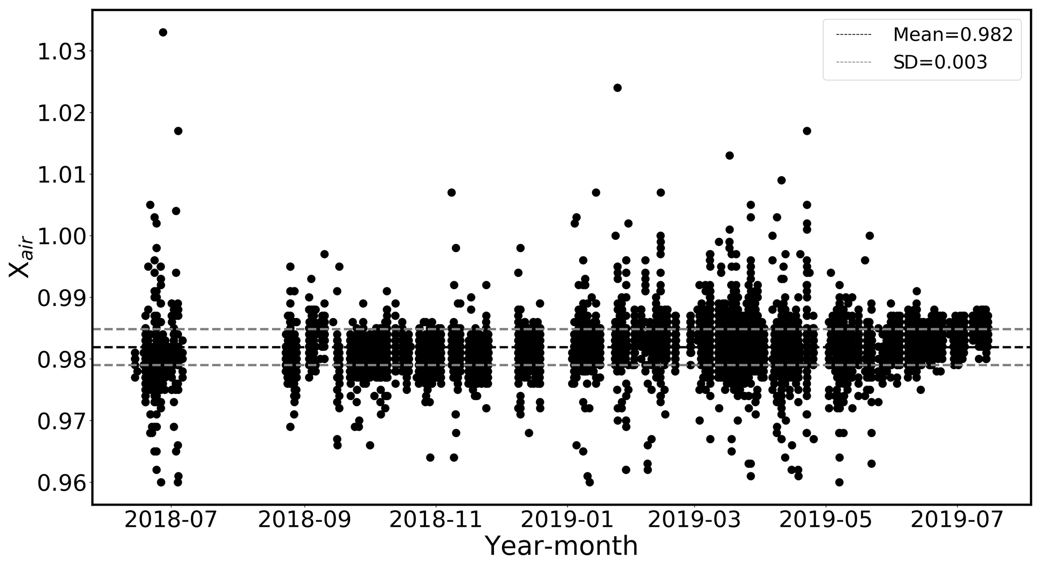
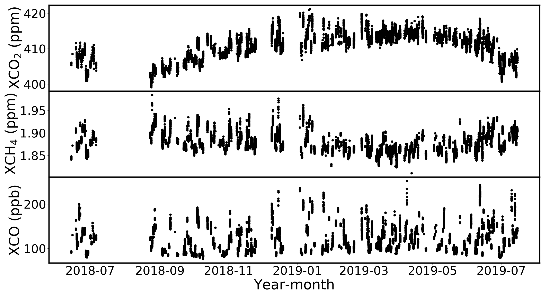
Figure 8Time series of XCO2, XCH4 and XCO covering the period from 14 June 2018 to 19 July 2019.
Similar day-to-day variations are observed among XCO2, XCH4 and XCO. The high values are related to the local emissions while the low values are influenced by the air transported from remote places. In this section, we use CO as a trace gas to evaluate the correlations between XCO and XCO2, XCO and XCH4. Figure 10a, b show the correlations between the XCO and XCO2 daily means and between the XCO and XCH4 daily means at Xianghe. XCO2 is high in winter and low in summer, and XCH4 is high in summer and autumn and low in winter. In order to reduce the impact from their seasonal variations, a linear regression model is used to fit the time series of measurements,
where Y(t) is the measurements of XCO2, XCH4 or XCO; A0 is the measurements (backgrounds); and A1–A6 are the amplitudes of the periodic variations during the year (seasonal variation). ΔY(t) is the measurement without background and seasonal variations, representing the day-to-day variation. Note that we assume there are no trends of these species due to a relatively short time coverage of about 1 year. Figure 10c, d show the correlations between the ΔXCO and ΔXCO2 daily means and between the ΔXCO and ΔXCH4 daily means. The correlation coefficient (R) between XCO and XCO2 increases from 0.50 to 0.66, and the R between XCO and XCH4 increases from 0.67 to 0.82. The seasonal variation in ΔXCO2 can still be observed, but the amplitude is much reduced. There is almost no seasonal variation in ΔXCH4. Figure 11 shows the correlations in each season. Good correlations between ΔXCO and ΔXCH4 are found for the whole year, with R in the range of 0.72–0.87. There is a good correlation (R>=0.85) between ΔXCO and ΔXCO2 in autumn and winter and a worse correlation (R=0.47) in spring and (R=0.57) in summer. It is assumed that the random distribution of the ΔXCO is symmetric, and the lowest ΔXCO is about −36 ppb. Therefore, each day with ΔXCO>36 ppb is classified as a polluted day and vice versa. In total, we have 28 polluted days and 187 clean days. FTIR measurements show ΔXCO, ΔXCO2 and ΔXCH4 are much larger on the polluted days than those on the clean days (see Table 3).
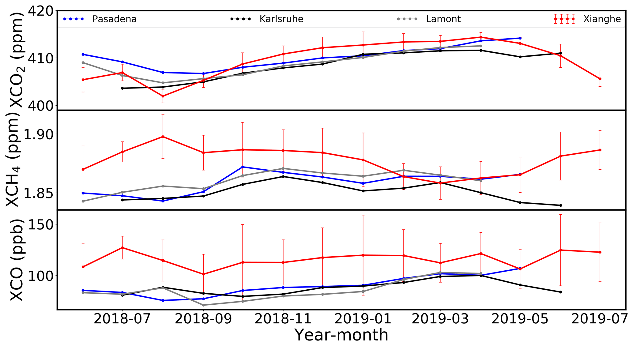
Figure 9Monthly mean of XCO2, XCH4 and XCO at Pasadena, Karlsruhe, Lamont and Xianghe. The error bars are the monthly SDs of XCO2, XCH4 and XCO at Xianghe.

Figure 10The correlation plots between the XCO and XCO2 and XCH4 daily means (a, b) and the correlation plots between the ΔXCO and ΔXCO2 and ΔXCH4 daily means (c, d) from FTIR TCCON-type measurements at Xianghe. The dashed red line is the linear fit. N is the number of the measurement days, and R is the correlation coefficient. The error bar is the SD of the measurements on each day. The data are colored with the measurement months.
The 10 d backward trajectories for polluted and clean days classified by CO measurements are also plotted using the Lagrangian particle dispersion model version 9.02 (FLEXPART) (Stohl et al., 2005). FLEXPART is able to simulate a large range of atmospheric transport processes, taking mean flow, deep convection and turbulence into account. The backward running of FLEXPART provides the release–receptor relationship, which is applied to study the source and transport of the observations from a measurement site. In this study, 20 000 air particles are released at Xianghe between 10:00 and 14:00 (local time) for days when FTIR measurements are available in the vertical range from the surface to 2 km (focusing on the atmospheric boundary layer due to a polluted site), and a 4-D response function to emission inventory is calculated. The model was driven by meteorological data from the European Centre for Medium-Range Weather Forecasts (ECMWF). The residence time of particles in output grid cells describes the sensitivity of the receptor to the source. Figure 12 shows the mean air sources for polluted and clean days. It is found that the air is mainly from the south and the local polluted region (north China) for the polluted days and is mainly from the north and remote clean places (Inner Mongolia, Mongolia and Russia) for the clean days.
Table 3The mean and SD of ΔXCO, ΔXCO2 and ΔXCH4 on polluted and clean days.
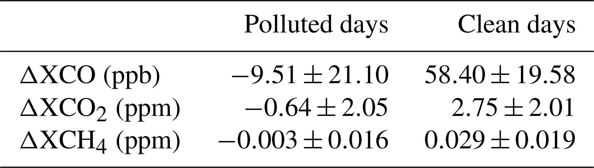
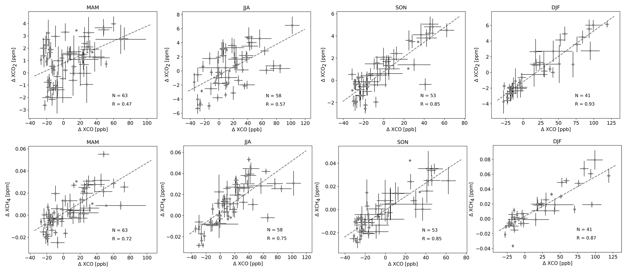
Figure 11Upper panels: the correlation plots between the ΔXCO and ΔXCO2 in four seasons (spring: March, April, May – MAM; summer: June, July, August – JJA; autumn: September, October, November – SON; winter: December, January, February – DJF). Lower panels: the correlation plots between the ΔXCO and ΔXCH4 in four seasons. The dashed line is the linear fit. N is the number of the measurement days, and R is the correlation coefficient. The error bar is the SD of the measurements in each day.
4.1 Methodology
In this section, the FTIR XCO2, XCH4 and XCO measurements at Xianghe are used to compare with the OCO-2 XCO2 and TROPOMI XCH4 and XCO satellite observations. There are 215 d measurements of 15 435 individual FTIR retrievals. The co-located FTIR–satellite data pairs are selected based on spatial–temporal collocation criteria. The detailed selection criteria for each target (OCO-2 XCO2, TROPOMI XCH4 and TROPOMI XCO) are described in Sect. 4.2 and 4.3: they account for the scan width of the satellite instrument and the characteristics of the target species.
According to Rodgers and Connor (2003), the differences in a priori profiles should be taken into account when comparing ground-based FTIR and satellite observations. TCCON CO2, CH4 and CO a priori profiles (70 layers) have been discussed in Sect. 3.1. OCO-2 CO2 a priori profiles (19 layers) are created based on the GlobalView dataset and change with time and location (O'Dell et al., 2012). TROPOMI uses the global chemical transport model TM5 to get CH4 and CO a priori profiles (12 layers) (Borsdorff et al., 2018; Hasekamp et al., 2019). The TM5 model data are monthly means with a horizontal resolution of 2∘ latitude × 3∘ longitude and 60 vertical levels (Krol et al., 2005). In this study, the satellite a priori profile (OCO-2 or TROPOMI) is taken to be the common a priori profile in the comparison. To substitute the satellite a priori profile in the FTIR retrieval, we follow Rodgers and Connor (2003):
where is the FTIR retrieved total column using the satellite a priori profile, XFTIR is the original FTIR retrieval, A is the FTIR TCCON column averaging kernel, I is the unit vector, and xa,FTIR and xa,SAT are the a priori partial column profiles of FTIR and satellite retrievals, respectively. As the vertical layering of the FTIR retrieval is different from that of the satellite retrieval (OCO-2 or TROPOMI), the satellite a priori profile is re-gridded to the FTIR layer. After re-gridding, the total a priori column remains unchanged (Langerock et al., 2015).
To compare the FTIR and satellite column measurements, the satellite measurements are corrected for a possible difference between the altitudes of its ground pixel and that of the FTIR site at Xianghe. If the surface altitude of the satellite footprint is higher than the altitude of the FTIR instrument, the FTIR a priori profile (xa,FTIR) is used to fill the gap between the satellite lowest level (Ps,SAT) and the FTIR height (Ps,FTIR); otherwise the satellite a priori profile is considered to be the profile between the lowest satellite level and the FTIR height. Then the partial column of dry air (PCdry,air) or target species (PCgas) between the satellite footprint surface altitude and the FTIR surface altitude is calculated as
where g(P) is gravitational acceleration at height P, x(P) is the a priori volume mixing ratio (VMR) profile of each target gas, and is the VMR of water vapor in the dry air, calculated as
where νh2o is the VMR of water vapor in the wet air. Then each satellite pixel measurement is scaled with one scaling factor (α) related to satellite pixel level, which is computed as
where TC and TC are the total columns of dry air and target species in the satellite measurement column. The random error of FTIR measurements together with the systematic and random errors of satellite measurements are considered here for the comparison.
4.2 OCO-2
OCO-2 incorporates three imaging grating spectrometers to measure near-infrared spectra. The spectral resolution of OCO-2 is approximately 20 times lower than that of the TCCON FTIR (0.02 cm−1) instruments (Frankenberg et al., 2015). OCO-2 collects eight soundings over its 0.8∘ swath width every 0.333 s with a 16 d repeat cycle (https://ocov2.jpl.nasa.gov/instrument/, last access: 11 July 2020). The OCO-2 XCO2 measurements are retrieved by the Atmospheric CO2 Observations from Space (ACOS) retrieval algorithm (O'Dell et al., 2012), based on the optimal estimation method. Three bands (0.756, 1.61 and 2.06 µm) are used in the XCO2 retrieval. The a priori surface pressure and profiles of temperature and water vapor are from 3-hourly ECMWF model forecast fields and linearly interpolated in space and time to the satellite footprint. Note that there are three versions (v7, v8 and v9) available on the NASA website for the OCO-2 data. Each version comes in two variants: full and lite. The full variant contains all the retrieved parameters, but without any post-correction applied to the data. The lite variant only includes some important parameters, but the data are corrected in terms of a footprint-dependent bias, a parameter-dependent bias and a scaling bias according to the WMO trace-gas standard scale. Compared to v7, many parameters have been improved in v8, such as latitude-dependent problems, surface model, spectroscopy, potential instrumental problems, atmospheric scattering by clouds and aerosols, a spatial–temporal sampling error of a priori surface pressure and the systematic pointing offsets (O'Dell et al., 2012). Based on v8, v9 has a better estimation of the surface pressure, and it shows a better performance in regions with rough topography such as over Lauder (New Zealand) (Kiel et al., 2019). In this study, the latest v9 lite data are selected (https://ocov2.jpl.nasa.gov, last access: 11 July 2020.).
The satellite measurements are selected within 5∘ latitude ×10∘ longitude around Xianghe; these are the same criteria as adopted by Wunch et al. (2017). For each FTIR measurement, the nearby satellite measurement in the spatial collocation box, with less than 2 h measurement time difference, is chosen to form one FTIR–satellite data pair. Note that there are nadir and glint observational modes of OCO-2 measurements over Xianghe, and these two types of measurements are combined together to get a statistically robust result with 28 data pairs.
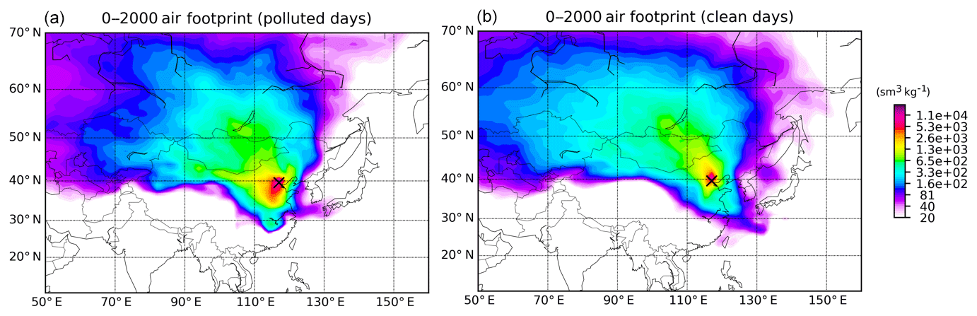
Figure 12The mean emission response sensitivities of the air mass at Xianghe (the cross symbol) for polluted (a) and clean (b) days in the vertical range from surface to 2000 m a.s.l. simulated with a 10 d backward run with FLEXPART v9.02.
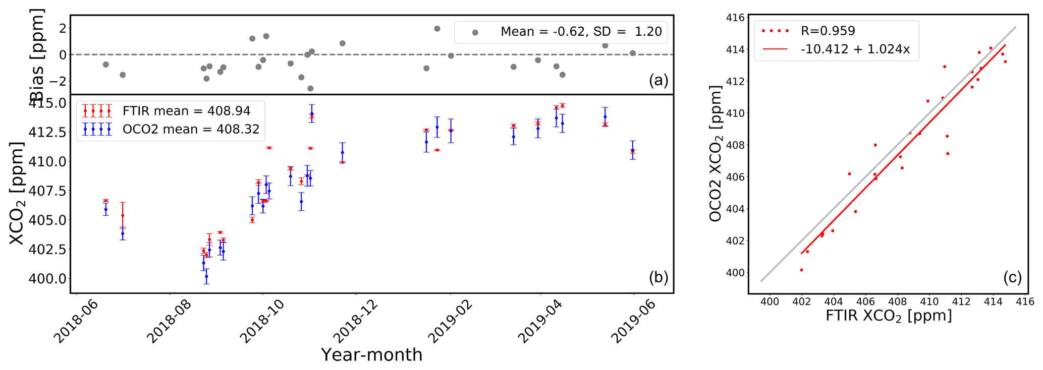
Figure 13(a, b) Time series of daily mean co-located OCO-2 and ground-based FTIR XCO2 data at Xianghe (b) and the bias between them (a). The error bars are the daily SDs of co-located OCO-2 and the FTIR instrument XCO2 data. (c) Correlation plot between co-located daily mean XCO2 data from OCO-2 and the FTIR instrument at Xianghe.
The time series of the co-located OCO-2 and ground-based FTIR data from 27 June 2018 to 31 May 2019 (last date of satellite data availability) is shown in Fig. 13. To avoid the influence from the cloud, we select the co-located data pair, which has at least 20 OCO-2 measurements within the box. Figure 13a shows the daily mean bias of measured XCO2 from OCO-2 and the FTIR instrument. The mean of OCO-2 measurements is 0.62 ppm lower than that of the FTIR measurements, with a SD of 1.20 ppm. The absolute differences between OCO-2 v9 lite data and Xianghe FTIR data are comparable with the results found for the v7 lite products in Wunch et al. (2017) for other TCCON stations with biases ranging from ppm (Wollongong) to 0.9±1.49 ppm (Karlsruhe) in land glint mode and ranging from ppm (Wollongong) to 1.6±2.05 ppm (Garmisch) in nadir mode. The scatter plot of OCO-2 and the FTIR instrument at Xianghe is shown in Fig. 13c: the derived correlation coefficient (R) is 0.959. We can conclude that OCO-2 data are in good agreement with the Xianghe FTIR data and in particular that OCO-2 captures the seasonal cycle of XCO2 at Xianghe, with a maximum in winter–spring and a minimum in late summer.
4.3 TROPOMI
In this section, the TROPOMI XCH4 and XCO are compared with the FTIR measurements at Xianghe. TROPOMI is a grating spectrometer measuring solar radiation reflected by the Earth and observes in the ultraviolet, visible, near-infrared and shortwave infrared spectral regions. It has a wide swath of around 2600 km across the track and a daily global coverage of the Earth. The spatial resolution of TROPOMI is about 7 km ×7 km before 6 August 2019 and then it changes to 7.2 km ×5.6 km. The TROPOMI CO data are provided in three different data streams: the near-real-time (NRTI) stream (since June 2018, with the same starting month as FTIR measurements at Xianghe), the offline stream (OFFL) and the reprocessing (RPRO) stream (Landgraf et al., 2020a). CH4 data are provided in bias-corrected and not-corrected versions (Landgraf et al., 2020b). In our validation, we considered the offline and reprocessed CO data, from processor versions 01.02 and higher. For CH4, we also look at bias-corrected data with processor versions of 01.02 and higher. The FTIR measurements at Xianghe can provide very useful information in the polluted area of north China, which is also important for TROPOMI product validation.
TROPOMI uses the RemoTeC algorithm to retrieve the CH4 column using the 0.757–0.774 µm O2 absorption band and 2.305–2.385 µm CH4 absorption band (Hasekamp et al., 2019). The requirements for the accuracy and precision for TROPOMI XCH4 are 1 % and 1.5 %, respectively (Hasekamp et al., 2019). We select TROPOMI XCH4 measurements that occur within 1 h of FTIR measurements and within a distance of 100 km from the Xianghe station based on the collocation criteria adopted at other TCCON sites (Lambert et al., 2019). In agreement with Landgraf et al. (2020b), the TROPOMI pixels are selected with a quality assurance value above 0.5, which removes pixels with processing errors, anomalously high signals and increasing specular reflection of sunlight by the sea surface (Hasekamp et al., 2019). Similar to OCO-2, to reduce the influence from the clouds, we only select the days when there are at least five co-located TROPOMI CH4 pixels.
Figure 14a, b show the time series of co-located TROPOMI and FTIR XCH4 daily means and their relative biases (percent, (satellite − FTIR)∕FTIR) from 27 June 2018 to 19 July 2019 (86 d). The co-located TROPOMI and FTIR XCH4 data pairs at Xianghe are distributed evenly in all seasons. The mean bias is −0.60 %, which is within the S5P validation requirements of a bias of 1 %. In addition, the SD of the relative biases is 0.55 %, which also meets the S5P mission requirement of 1.5 % (Lambert et al., 2019). The R between TROPOMI and FTIR XCH4 daily means is 0.834 (Fig. 14c). According to the TROPOMI validation report (Lambert et al., 2019), the bias at Xianghe is comparable to the ones at Tsukuba, Lamont and Rikubetsu (similar latitude band).
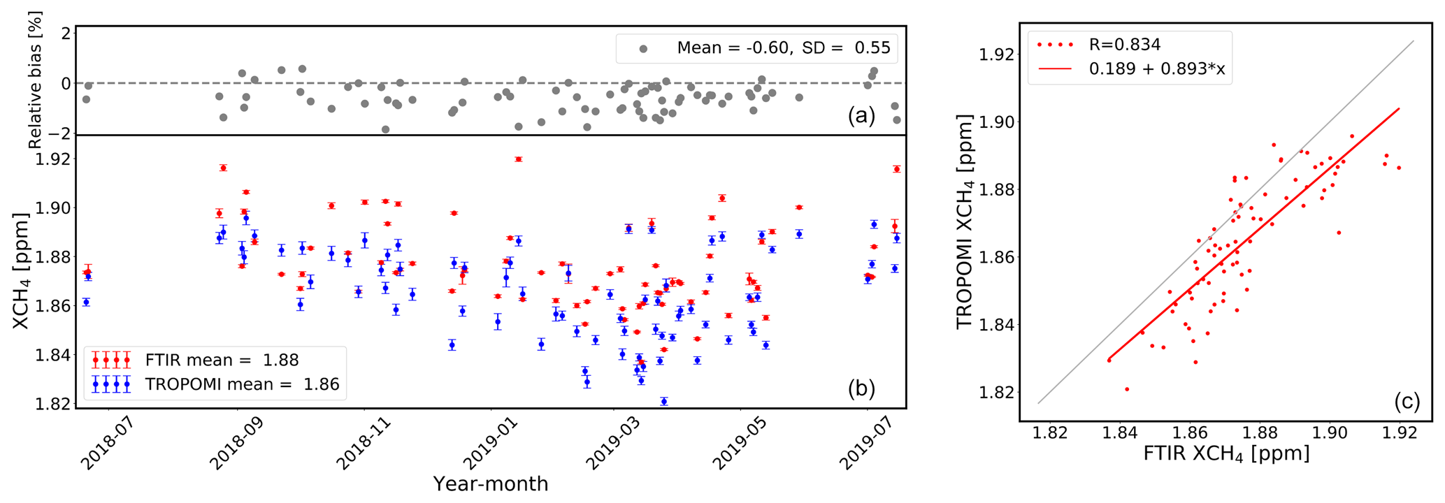
Figure 14(a, b) Time series of daily mean co-located TROPOMI and ground-based FTIR XCH4 data at Xianghe (b) and the relative bias between them (a). The error bars are the relative SDs of co-located TROPOMI and FTIR XCH4 data. (c) Correlation plot between co-located daily mean XCH4 data from TROPOMI and the FTIR instrument at Xianghe.
The TROPOMI XCO measurements are retrieved from the shortwave infrared CO removal (SICOR) algorithm (Hasekamp et al., 2019) in the 2.3 µm spectral range. The retrieved TROPOMI CO data are in the unit of total column density (molecules cm−2), so we converted them to XCO (ppb) values for comparison with FTIR XCO measurements (Langerock et al., 2015):
where XCO is the total column-averaged dry-air mole fraction of TROPOMI CO measurements. TCCO is the total column density of TROPOMI CO measurements, and TC is total column density of dry air in the satellite measurement column. Because CO is relatively reactive compared to CH4, we must reduce the measurement time and location differences in the colocation criteria. Therefore, the TROPOMI observations are selected within 30 min of each FTIR measurement and within a maximum distance of 50 km away from the FTIR site and along the light path of the ground-based FTIR measurements. Similar to CH4, we only select the days when there are at least five co-located TROPOMI CO pixels. In addition, to reduce the impact from long light paths through the atmosphere (Landgraf et al., 2020a), the TROPOMI measurements with a SZA larger than 80∘ or a satellite zenith angle larger than 65∘ are filtered out. And we only select the TROPOMI CO products in clear-sky cases with cloud height below 500 m and cloud optical depth <0.5.
Figure 15a, b show the time series and relative biases of co-located TROPOMI and FTIR XCO daily means at Xianghe from 27 June 2018 to 31 May 2019 (70 d). In addition, the co-located TROPOMI and FTIR XCO data pairs at Xianghe are also distributed evenly in all seasons. The mean bias and SD between TROPOMI and the FTIR instrument are 2.05 % and 7.82 %, respectively, which are within the S5P mission requirements (bias <15 % and SD <10 %). Compared to other TCCON sites (Lambert et al., 2019), the mean relative bias is relatively low. The good agreement between TROPOMI and FTIR XCO with a R of 0.961 (Fig. 15c) highlights the good performance of TROPOMI over Xianghe.
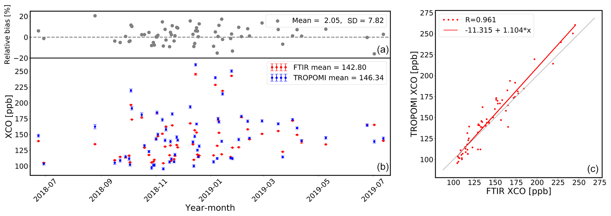
Figure 15(a, b) Time series of daily mean co-located TROPOMI and ground-based FTIR XCO data at Xianghe (b) and the relative bias between them (a). The error bars are the relative SDs of co-located TROPOMI and FTIR XCO data. (c) Correlation plot between co-located daily mean XCO data from TROPOMI and the FTIR instrument at Xianghe.
A new ground-based FTIR Bruker 125HR instrument has been in operation since 14 June 2018 at Xianghe (39.75∘ N, 116.96∘ E) in north China. It performs NIR solar absorption measurements of XCO2, XCH4 and XCO following the TCCON operation and data analysis procedures since June 2018. Regular HCl cell measurements show that the ME loss is within 5 % for the whole time period, and the PE deviation remains within 0.02 rad most of the time, confirming that the ILS of the FTIR spectrometer is stable and meets the TCCON requirements. XCO2, XCH4 and XCO have been retrieved using the current TCCON standard algorithm GGG2014.
Because the InGaAs spectra have been recorded in AC mode before 31 May 2019 and AC + DC mode afterwards, we designed a filtering method based on SNR and SI. Application of this filtering to the spectra in AC mode shows that about 85 % of the spectra have the required quality. The thus achieved precision of < 0.8 ppm for the retrieved XCO2 complies with the TCCON requirements, demonstrating that the SI filtering can overcome the absence of the DC signal.
During this 1-year period of measurements, a clear seasonal variation in XCO2 has been observed, with the lowest values of 401.95±1.43 ppm in summer and the highest values of 414.37±0.97 ppm in winter. Low XCH4 concentrations are observed in spring (1.858±0.014 ppm), and high values are observed in autumn and summer (1.898±0.019 ppm). For XCO there is no clear seasonal variation but a large day-to-day variability. According to the FTIR measurements, it is found that the high values of XCO2, XCH4 and XCO are highly related.
Comparisons between the XCO2, XCH4 and XCO FTIR measurements at Xianghe and satellite data illustrate that this site is an interesting additional site for satellite validation in northern China. The mean bias between FTIR and OCO-2 XCO2 measurements is −0.62 ppm with a SD of 1.20 ppm. The mean and SD of the relative differences between FTIR and TROPOMI XCH4 measurements are −0.60 % and 0.55 %, respectively. Both results are consistent with comparisons between these satellite data and other TCCON sites. The mean and SD of the relative differences between FTIR and TROPOMI XCO measurements are 2.05 % and 7.82 %, respectively, which is within the S5P mission requirements. However, the mean relative bias is lower than what is observed at other TCCON sites. This is probably due to the fact that the a priori profile in the TROPOMI retrieval is overestimated at Xianghe. The seasonal and synoptic variations in XCO are however well captured by TROPOMI. The ground-based FTIR measurements at Xianghe are demonstrated to be very useful to evaluate the performance of the greenhouse gases observing satellites (OCO-2 and TROPOMI) in this region.
In summary, this study shows that the ground-based FTIR Xianghe data for XCO2, XCH4 and XCO comply with the TCCON specifications. The objective is to become a TCCON-affiliated site in the future. As Xianghe is a rather polluted location, it can provide useful information for the study of the carbon cycle in north China and for the validation of satellite observations.
The Xianghe FTIR CO2, CH4 and CO data can be accessed at https://doi.org/10.18758/71021049 (Yang et al., 2019). The OCO-2 data are publicly available (https://doi.org/10.5067/VWSABTO7ZII4, OCO-2 Science Team et al., 2020). The TROPOMI data are publicly available (https://doi.org/10.5270/S5P-3p6lnwd, ESA, 2019 and https://doi.org/10.5270/S5P-1hkp7rp, ESA, 2018).
MZ, PW, GW and MDM designed the experiment. YY, MZ, CH, TW, DJ, CV and NK operated and maintained the FTIR instruments. YY, MZ, BL and MKS performed the satellite validation. YY and MZ wrote the manuscript, and all authors read and provided comments on the paper.
The authors declare that they have no conflict of interest.
We want to thank the TCCON community for providing the retrieval code (GGG2014), and sharing all their FTIR knowledge. We also want to thank Weidong Nan, Qun Cheng and Qing Yao at the Xianghe site and Rongshi Zou (IAP) and Francis Scolas for the FTIR maintenance.
The work is supported by the National Key R & D Program of China (nos. 2017YFB0504000 and 2017YFC1501701), the National Natural Science Foundation of China (no. 41575034) and the China Scholarship Council.
This paper was edited by Jens Klump and reviewed by three anonymous referees.
Andres, R. J., Boden, T. A., Bréon, F.-M., Ciais, P., Davis, S., Erickson, D., Gregg, J. S., Jacobson, A., Marland, G., Miller, J., Oda, T., Olivier, J. G. J., Raupach, M. R., Rayner, P., and Treanton, K.: A synthesis of carbon dioxide emissions from fossil-fuel combustion, Biogeosciences, 9, 1845–1871, https://doi.org/10.5194/bg-9-1845-2012, 2012. a
Beer, R.: Remote Sensing by Fourier Transform Spectrometry, Wiley-Interscience, New York, 120, 1992. a
Borsdorff, T., Aan de Brugh, J., Hu, H., Aben, I., Hasekamp, O., and Landgraf, J.: Measuring Carbon Monoxide With TROPOMI: First Results and a Comparison With ECMWF-IFS Analysis Data, Geophys. Res. Lett., 45, 2826–2832, https://doi.org/10.1002/2018GL077045, 2018. a, b, c
Crisp, D., Atlas, R., Breon, F.-M., Brown, L., Burrows, J., Ciais, P., Connor, B., Doney, S., Fung, I., Jacob, D., Miller, C., O’Brien, D., Pawson, S.and Randerson, J., Rayner, P., Salawitch, R., Sander, S., Sen, B., Stephens, G. L., Tans, P. P., Toon, G. C., Wennberg, P. O., Wofsy, S. C., Yung, Y. L., Kuang, Z., Chudasama, B., Sprague, G., Weiss, B., Pollock, R., Kenyon, D., and Schroll, S.: The Orbiting Carbon Observatory (OCO) mission, Adv. Space. Res., 34, 700–709, https://doi.org/10.1016/j.asr.2003.08.062, 2004. a
Crisp, D., Pollock, H. R., Rosenberg, R., Chapsky, L., Lee, R. A. M., Oyafuso, F. A., Frankenberg, C., O'Dell, C. W., Bruegge, C. J., Doran, G. B., Eldering, A., Fisher, B. M., Fu, D., Gunson, M. R., Mandrake, L., Osterman, G. B., Schwandner, F. M., Sun, K., Taylor, T. E., Wennberg, P. O., and Wunch, D.: The on-orbit performance of the Orbiting Carbon Observatory-2 (OCO-2) instrument and its radiometrically calibrated products, Atmos. Meas. Tech., 10, 59–81, https://doi.org/10.5194/amt-10-59-2017, 2017. a, b
ESA: TROPOMI Level 2 Carbon Monoxide total column products, Version 01, European Space Agency, https://doi.org/10.5270/S5P-1hkp7rp, 2018. a
ESA: TROPOMI Level 2 Methane Total Column products, Version 01, European Space Agency, https://doi.org/10.5270/S5P-3p6lnwd 2019. a
Eldering, A., O'Dell, C. W., Wennberg, P. O., Crisp, D., Gunson, M. R., Viatte, C., Avis, C., Braverman, A., Castano, R., Chang, A., Chapsky, L., Cheng, C., Connor, B., Dang, L., Doran, G., Fisher, B., Frankenberg, C., Fu, D., Granat, R., Hobbs, J., Lee, R. A. M., Mandrake, L., McDuffie, J., Miller, C. E., Myers, V., Natraj, V., O'Brien, D., Osterman, G. B., Oyafuso, F., Payne, V. H., Pollock, H. R., Polonsky, I., Roehl, C. M., Rosenberg, R., Schwandner, F., Smyth, M., Tang, V., Taylor, T. E., To, C., Wunch, D., and Yoshimizu, J.: The Orbiting Carbon Observatory-2: first 18 months of science data products, Atmos. Meas. Tech., 10, 549–563, https://doi.org/10.5194/amt-10-549-2017, 2017. a
Feist, D. G., Arnold, S. G., Hase, F., and Ponge, D.: Rugged optical mirrors for Fourier transform spectrometers operated in harsh environments, Atmos. Meas. Tech., 9, 2381–2391, https://doi.org/10.5194/amt-9-2381-2016, 2016. a
Frankenberg, C., Pollock, R., Lee, R. A. M., Rosenberg, R., Blavier, J.-F., Crisp, D., O'Dell, C. W., Osterman, G. B., Roehl, C., Wennberg, P. O., and Wunch, D.: The Orbiting Carbon Observatory (OCO-2): spectrometer performance evaluation using pre-launch direct sun measurements, Atmos. Meas. Tech., 8, 301–313, https://doi.org/10.5194/amt-8-301-2015, 2015. a
Gisi, M., Hase, F., Dohe, S., and Blumenstock, T.: Camtracker: a new camera controlled high precision solar tracker system for FTIR-spectrometers, Atmos. Meas. Tech., 4, 47–54, https://doi.org/10.5194/amt-4-47-2011, 2011. a
Gregg, J. S., Andres, R. J., and Marland, G.: China: Emissions pattern of the world leader in CO2 emissions from fossil fuel consumption and cement production, Geophys. Res. Lett., 35, L08806, https://doi.org/10.1029/2007GL032887, 2008. a
Hase, F., Blumenstock, T., and Paton-Walsh, C.: Analysis of the instrumental line shape of high-resolution Fourier transform IR spectrometers with gas cell measurements and new retrieval software, Appl. Opt., 38, 3417–3422, https://doi.org/10.1364/AO.38.003417, 1999. a
Hase, F., Drouin, B. J., Roehl, C. M., Toon, G. C., Wennberg, P. O., Wunch, D., Blumenstock, T., Desmet, F., Feist, D. G., Heikkinen, P., De Mazière, M., Rettinger, M., Robinson, J., Schneider, M., Sherlock, V., Sussmann, R., Té, Y., Warneke, T., and Weinzierl, C.: Calibration of sealed HCl cells used for TCCON instrumental line shape monitoring, Atmos. Meas. Tech., 6, 3527–3537, https://doi.org/10.5194/amt-6-3527-2013, 2013. a
Hase, F., Blumenstock, T., Dohe, S., Gross, J., and Kiel, M.: TCCON data from Karlsruhe (DE), Release GGG2014R0, TCCON data archive, hosted by CaltechDATA, https://doi.org/10.14291/tccon.ggg2014.karlsruhe01.R0/1149270, 2014. a
Hasekamp, O., Lorente, A., Hu, H., Butz, A., de Brugh, J., and Landgraf, J.: Algorithm Theoretical Baseline Document for Sentinel-5 Precursor Methane Retrieval, Netherlands Institute for Space Research, p. 67, available at: http://www.tropomi.eu/sites/default/files/files/publicSentinel-5P-TROPOMI-ATBD-Methane-retrieval.pdf (last access: 11 July 2020), 2019. a, b, c, d, e
IPCC: Climate change 2013: The physical science basis, Contribution of Working Group I to the Fifth Assessment Report of the Intergovernmental Panel on Climate Change, available at: https://www.ipcc.ch/report/ar5/wg1/ (last access: 11 July 2020), 2013. a, b
Jackson, R. B., Le Quéré, C., Andrew, R. M., Canadell, J. G., Peters, G. P., Roy, J., and Wu, L.: Warning signs for stabilizing global CO2 emissions, Environ. Res. Lett., 12, 110202, https://doi.org/10.1088/1748-9326/aa9662, 2017. a
Kalnay, E., Kanamitsu, M., Kistler, R., Collins, W., Deaven, D., Gandin, L., Iredell, M., Saha, S., White, G., Woollen, J., Zhu, Y., Chelliah, M., Ebisuzaki, W., Higgins, W., Janowiak, J., Mo, K. C., Ropelewski, C., Wang, J., Leetmaa, A., Reynolds, R., Jenne, R., and Joseph, D.: The NCEP/NCAR 40-Year Reanalysis Project, B. Am. Meteorol. Soc., 77, 437–472, https://doi.org/10.1175/1520-0477(1996)077<0437:TNYRP>2.0.CO;2, 1996. a
Keppel-Aleks, G., Toon, G. C., Wennberg, P. O., and Deutscher, N. M.: Reducing the impact of source brightness fluctuations on spectra obtained by Fourier-transform spectrometry, Appl. Opt., 46, 4774–4779, https://doi.org/10.1364/AO.46.004774, 2007. a
Keppel-Aleks, G., Wennberg, P. O., and Schneider, T.: Sources of variations in total column carbon dioxide, Atmos. Chem. Phys., 11, 3581–3593, https://doi.org/10.5194/acp-11-3581-2011, 2011. a
Kiel, M., O'Dell, C. W., Fisher, B., Eldering, A., Nassar, R., MacDonald, C. G., and Wennberg, P. O.: How bias correction goes wrong: measurement of XCO2 affected by erroneous surface pressure estimates, Atmos. Meas. Tech., 12, 2241–2259, https://doi.org/10.5194/amt-12-2241-2019, 2019. a
Kirschke, S., Bousquet, P., Ciais, P., Saunois, M., Canadell, J. G., Dlugokencky, E. J., Bergamaschi, P., Bergmann, D., Blake, D. R., B., Bruhwiler, L., Cameron-Smith, P., Castaldi, S., Chevallier, F., Feng, L., Fraser, A., M., H., Hodson, E. L., Houweling, S., Josse, B., Fraser, P. J., Krummel, P. B., Lamarque, J. F., Langenfelds, R. L., Le Quéré, C., Naik, V., O'Doherty, S., Palmer, P. I., Pison, I., Plummer, D., Poulter, b., Prinn, R. G., Rigby, M., Ringeval, B., Santini, M., Schmidt, M., Shindell, D. T., Simpson, I. J., Spahni, R., Steele, L. P., Strode, S. A., Sudo, K., Szopa, S., Van der Werf, G. R., Voulgarakis, A., Van Weele, M., Weiss, R. F., Williams, J. E., and Zeng, G.: Three decades of global methane sources and sinks, Nat. Geosci., 6, 813–823, https://doi.org/10.1038/ngeo1955, 2013. a
Kivi, R. and Heikkinen, P.: Fourier transform spectrometer measurements of column CO2 at Sodankylä, Finland, Geosci. Instrum. Method. Data Syst., 5, 271–279, https://doi.org/10.5194/gi-5-271-2016, 2016. a
Krol, M., Houweling, S., Bregman, B., van den Broek, M., Segers, A., van Velthoven, P., Peters, W., Dentener, F., and Bergamaschi, P.: The two-way nested global chemistry-transport zoom model TM5: algorithm and applications, Atmos. Chem. Phys., 5, 417–432, https://doi.org/10.5194/acp-5-417-2005, 2005. a
Kuze, A., Suto, H., Nakajima, M., and Hamazaki, T.: Thermal and near infrared sensor for carbon observation Fourier-transform spectrometer on the Greenhouse Gases Observing Satellite for greenhouse gases monitoring, Appl. Opt., 48, 6716–6733, https://doi.org/10.1364/AO.48.006716, 2009. a
Lambert, J. C., Keppens, A., Hubert, D., Langerock, B., Eichmann, K., Kleipool, Q., Sneep, M., Verhoelst, T., Wagner, T., Weber, M., Ahn, C., Argyrouli, A., Balis, D., Chan, K., Compernolle, S., De Smedt, I., Eskes, H., Fjæraa, A., Garane, K., and et al.: Quarterly Validation Report of the CopernicusSentinel-5 PrecursorOperational Data Products #03: July 2018–May 2019, S5P MPC Routine Operations Consolidated Validation Reportseries, 3, 1–125, available at: http://www.tropomi.eu/sites/default/files/files/publicS5P-MPC-IASB-ROCVR-03.0.1-20190621_FINAL.pdf (last access: 11 July 2020), 2019. a, b, c, d, e
Landgraf, J., Borsdorff, T., Langerock, B., and Keppens, A.: S5P Mission Performance Centre Carbon Monoxide [L2__CO____] Readme, available at: https://sentinel.esa.int/documents/247904/3541451/Sentinel-5P-Carbon-Monoxide-Level-2-Product-Readme-File, last access: 11 July 2020a. a, b
Landgraf, J., Lorente, A., Langerock, B., and Sha, M. K.: S5P Mission Performance Centre Methane [L2__CH4___] Readme, https://sentinel.esa.int/documents/247904/3541451/Sentinel-5P-Methane-Product-Readme-File, last access: 11 July 2020b. a, b
Langerock, B., De Mazière, M., Hendrick, F., Vigouroux, C., Desmet, F., Dils, B., and Niemeijer, S.: Description of algorithms for co-locating and comparing gridded model data with remote-sensing observations, Geosci. Model Dev., 8, 911–921, https://doi.org/10.5194/gmd-8-911-2015, 2015. a, b
Le Quéré, C., Andrew, R. M., Friedlingstein, P., Sitch, S., Hauck, J., Pongratz, J., Pickers, P. A., Korsbakken, J. I., Peters, G. P., Canadell, J. G., Arneth, A., Arora, V. K., Barbero, L., Bastos, A., Bopp, L., Chevallier, F., Chini, L. P., Ciais, P., Doney, S. C., Gkritzalis, T., Goll, D. S., Harris, I., Haverd, V., Hoffman, F. M., Hoppema, M., Houghton, R. A., Hurtt, G., Ilyina, T., Jain, A. K., Johannessen, T., Jones, C. D., Kato, E., Keeling, R. F., Goldewijk, K. K., Landschützer, P., Lefèvre, N., Lienert, S., Liu, Z., Lombardozzi, D., Metzl, N., Munro, D. R., Nabel, J. E. M. S., Nakaoka, S., Neill, C., Olsen, A., Ono, T., Patra, P., Peregon, A., Peters, W., Peylin, P., Pfeil, B., Pierrot, D., Poulter, B., Rehder, G., Resplandy, L., Robertson, E., Rocher, M., Rödenbeck, C., Schuster, U., Schwinger, J., Séférian, R., Skjelvan, I., Steinhoff, T., Sutton, A., Tans, P. P., Tian, H., Tilbrook, B., Tubiello, F. N., van der Laan-Luijkx, I. T., van der Werf, G. R., Viovy, N., Walker, A. P., Wiltshire, A. J., Wright, R., Zaehle, S., and Zheng, B.: Global Carbon Budget 2018, Earth Syst. Sci. Data, 10, 2141–2194, https://doi.org/10.5194/essd-10-2141-2018, 2018. a, b
Neefs, E., De Mazière, M., Scolas, F., Hermans, C., and Hawat, T.: BARCOS, an automation and remote control system for atmospheric observations with a Bruker interferometer, Rev. Sci. Instrum., 78, 035109, https://doi.org/10.1063/1.2437144, 2007. a
OCO-2 Science Team, Gunson, M., and Eldering, A.: ACOS GOSAT/TANSO-FTS Level 2 bias-corrected XCO2 and other select fields from the full-physics retrieval aggregated as daily files V9r, Greenbelt, MD, USA, Goddard Earth Sciences Data and Information Services Center (GES DISC), https://doi.org/10.5067/VWSABTO7ZII4, 2020. a
O'Dell, C. W., Connor, B., Bösch, H., O'Brien, D., Frankenberg, C., Castano, R., Christi, M., Eldering, D., Fisher, B., Gunson, M., McDuffie, J., Miller, C. E., Natraj, V., Oyafuso, F., Polonsky, I., Smyth, M., Taylor, T., Toon, G. C., Wennberg, P. O., and Wunch, D.: The ACOS CO2 retrieval algorithm – Part 1: Description and validation against synthetic observations, Atmos. Meas. Tech., 5, 99–121, https://doi.org/10.5194/amt-5-99-2012, 2012. a, b, c
Olsen, S. C., and Randerson, J. T.: Differences between surface and column atmospheric CO2 and implications for carbon cycle research, J. Geophys. Res.-Atmos., 109, D02301, https://doi.org/10.1029/2003JD003968, 2004. a
Ostler, A., Sussmann, R., Patra, P. K., Houweling, S., De Bruine, M., Stiller, G. P., Haenel, F. J., Plieninger, J., Bousquet, P., Yin, Y., Saunois, M., Walker, K. A., Deutscher, N. M., Griffith, D. W. T., Blumenstock, T., Hase, F., Warneke, T., Wang, Z., Kivi, R., and Robinson, J.: Evaluation of column-averaged methane in models and TCCON with a focus on the stratosphere, Atmos. Meas. Tech., 9, 4843–4859, https://doi.org/10.5194/amt-9-4843-2016, 2016. a
Peters, G. P., Marland, G., Corinne Le Quéré, Boden, T., Canadell, J. G., and Raupach, M. R.: Rapid growth in CO2 emissions after the 2008–2009 global financial crisis, Nat. Clim. Chang., 2, 2–4, https://doi.org/10.1038/nclimate1332, 2012. a
Pollard, D. F., Sherlock, V., Robinson, J., Deutscher, N. M., Connor, B., and Shiona, H.: The Total Carbon Column Observing Network site description for Lauder, New Zealand, Earth Syst. Sci. Data, 9, 977–992, https://doi.org/10.5194/essd-9-977-2017, 2017. a
Ran, L., Deng, Z., Wang, P., and Xia, X.: Black carbon and wavelength-dependent aerosol absorption in the North China Plain based on two-year aethalometer measurements, Atmos Environ., 142, 132–144, https://doi.org/10.1016/j.atmosenv.2016.07.014, 2016. a
Ridder, T., Warneke, T., and Notholt, J.: Source brightness fluctuation correction of solar absorption fourier transform mid infrared spectra, Atmos. Meas. Tech., 4, 1045–1051, https://doi.org/10.5194/amt-4-1045-2011, 2011. a
Rodgers, C. D. and Connor, B. J.: Intercomparison of remote sounding instruments, J. Geophys. Res.-Atmos., 108, 4116, https://doi.org/10.1029/2002JD002299, 2003. a, b
Schneider, M., Hase, F., Blumenstock, T., Redondas, A., and Cuevas, E.: Quality assessment of O3 profiles measured by a state-of-the-art ground-based FTIR observing system, Atmos. Chem. Phys., 8, 5579–5588, https://doi.org/10.5194/acp-8-5579-2008, 2008. a
Song, Y. L., Achberger, C., and Linderholm, H. W.: Rain-season trends in precipitation and their effect in different climate regions of China during 1961–2008, Environ. Res. Lett., 6, 034025, https://doi.org/10.1088/1748-9326/6/3/034025, 2011. a
Stohl, A., Forster, C., Frank, A., Seibert, P., and Wotawa, G.: Technical note: The Lagrangian particle dispersion model FLEXPART version 6.2, Atmos. Chem. Phys., 5, 2461–2474, https://doi.org/10.5194/acp-5-2461-2005, 2005. a
Toon, G., Blavier, J.-F., Washenfelder, R., Wunch, D., Keppel-Aleks, G., Wennberg, P., Connor, B., Sherlock, V., Griffith, D., Deutscher, N., and Notholt, J.: Total Column Carbon Observing Network (TCCON), OSA, https://doi.org/10.1364/FTS.2009.JMA3, 2009. a
Toon, G. C.: Atmospheric Line List for the 2014 TCCON Data Release, CaltechDATA, https://doi.org/10.14291/tccon.ggg2014.atm.r0/1221656, 2017. a
Toon, G. C. and Wunch, D.: A stand-alone a priori profile generation tool for GGG2014 release, CaltechDATA, https://doi.org/10.14291/tccon.ggg2014.priors.r0/1221661, 2015. a
Velazco, V. A., Deutscher, N. M., Morino, I., Uchino, O., Bukosa, B., Ajiro, M., Kamei, A., Jones, N. B., Paton-Walsh, C., and Griffith, D. W. T.: Satellite and ground-based measurements of XCO2 in a remote semiarid region of Australia, Earth Syst. Sci. Data, 11, 935–946, https://doi.org/10.5194/essd-11-935-2019, 2019. a
Washenfelder, R. A., Toon, G. C., Blavier, J.-F., Yang, Z., Allen, N. T., Wennberg, P. O., Vay, S. A., Matross, D. M., and Daube, B. C.: Carbon dioxide column abundances at the Wisconsin Tall Tower site, J. Geophys. Res.-Atmos., 111, D22305, https://doi.org/10.1029/2006JD007154, 2006. a
Wennberg, P. O., Wunch, D., Roehl, C., Blavier, J.-F., Toon, G. C., and Allen, N.: TCCON data from Caltech (US), Release GGG2014R1, TCCON data archive, CaltechDATA, https://doi.org/10.14291/tccon.ggg2014.pasadena01.R1/1182415, 2014. a
Wennberg, P. O., Wunch, D., Roehl, C., Blavier, J.-F., Toon, G. C., Allen, N., Dowell, P., Teske, K., Martin, C., and Martin., J.: TCCON data from Lamont (US), Release GGG2014R1, TCCON data archive, CaltechDATA, https://doi.org/10.14291/tccon.ggg2014.lamont01.R1/1255070, 2016. a
WMO: WMO Greenhouse Gas Bullitin, 14, available at: https://library.wmo.int/index.php?lvl=notice_display&id=20697#.XcMDaONpxGQ (last access: 11 July 2020), 2018. a, b
Wunch, D., Toon, G. C., Wennberg, P. O., Wofsy, S. C., Stephens, B. B., Fischer, M. L., Uchino, O., Abshire, J. B., Bernath, P., Biraud, S. C., Blavier, J.-F. L., Boone, C., Bowman, K. P., Browell, E. V., Campos, T., Connor, B. J., Daube, B. C., Deutscher, N. M., Diao, M., Elkins, J. W., Gerbig, C., Gottlieb, E., Griffith, D. W. T., Hurst, D. F., Jiménez, R., Keppel-Aleks, G., Kort, E. A., Macatangay, R., Machida, T., Matsueda, H., Moore, F., Morino, I., Park, S., Robinson, J., Roehl, C. M., Sawa, Y., Sherlock, V., Sweeney, C., Tanaka, T., and Zondlo, M. A.: Calibration of the Total Carbon Column Observing Network using aircraft profile data, Atmos. Meas. Tech., 3, 1351–1362, https://doi.org/10.5194/amt-3-1351-2010, 2010. a, b
Wunch, D., Toon, G. C., Blavier, J.-F. L., Washenfelder, R. A., Notholt, J., Connor, B. J., Griffith, D. W. T., Sherlock, V., and Wennberg, P. O.: The Total Carbon Column Observing Network, Philos. T. R. Soc. A., 369, 2087–2112, https://doi.org/10.1098/rsta.2010.0240, 2011a. a, b
Wunch, D., Wennberg, P. O., Toon, G. C., Connor, B. J., Fisher, B., Osterman, G. B., Frankenberg, C., Mandrake, L., O'Dell, C., Ahonen, P., Biraud, S. C., Castano, R., Cressie, N., Crisp, D., Deutscher, N. M., Eldering, A., Fisher, M. L., Griffith, D. W. T., Gunson, M., Heikkinen, P., Keppel-Aleks, G., Kyrö, E., Lindenmaier, R., Macatangay, R., Mendonca, J., Messerschmidt, J., Miller, C. E., Morino, I., Notholt, J., Oyafuso, F. A., Rettinger, M., Robinson, J., Roehl, C. M., Salawitch, R. J., Sherlock, V., Strong, K., Sussmann, R., Tanaka, T., Thompson, D. R., Uchino, O., Warneke, T., and Wofsy, S. C.: A method for evaluating bias in global measurements of CO2 total columns from space, Atmos. Chem. Phys., 11, 12317–12337, https://doi.org/10.5194/acp-11-12317-2011, 2011b. a, b
Wunch, D., Toon, G. C., Sherlock, V., Deutscher, N. M., Liu, C., Feist, D. G., and Wennberg, P. O.: Documentation for the 2014 TCCON Data Release, CaltechDATA, https://doi.org/10.14291/tccon.ggg2014.documentation.r0/1221662, 2015. a, b, c, d
Wunch, D., Wennberg, P. O., Osterman, G., Fisher, B., Naylor, B., Roehl, C. M., O'Dell, C., Mandrake, L., Viatte, C., Kiel, M., Griffith, D. W. T., Deutscher, N. M., Velazco, V. A., Notholt, J., Warneke, T., Petri, C., De Maziere, M., Sha, M. K., Sussmann, R., Rettinger, M., Pollard, D., Robinson, J., Morino, I., Uchino, O., Hase, F., Blumenstock, T., Feist, D. G., Arnold, S. G., Strong, K., Mendonca, J., Kivi, R., Heikkinen, P., Iraci, L., Podolske, J., Hillyard, P. W., Kawakami, S., Dubey, M. K., Parker, H. A., Sepulveda, E., García, O. E., Te, Y., Jeseck, P., Gunson, M. R., Crisp, D., and Eldering, A.: Comparisons of the Orbiting Carbon Observatory-2 (OCO-2) measurements with TCCON, Atmos. Meas. Tech., 10, 2209–2238, https://doi.org/10.5194/amt-10-2209-2017, 2017. a, b, c
Yang, Y., Zhou, M., Langerock, B., Sha, M., Hermans, C., Wang, T., Ji, D., Vigouroux, C., Kumps, N., Wang, G., De Mazière, M., and Wang, P.: Ground-based FTIR CO2, CH4 and CO measurements at Xianghe, China, Institute of Atmospheric Physics, https://doi.org/10.18758/71021049, 2019. a, b, c
Yin, Y., Chevallier, F., Ciais, P., Broquet, G., Fortems-Cheiney, A., Pison, I., and Saunois, M.: Decadal trends in global CO emissions as seen by MOPITT, Atmos. Chem. Phys., 15, 13433–13451, https://doi.org/10.5194/acp-15-13433-2015, 2015. a
Zheng, B., Chevallier, F., Ciais, P., Yin, Y., Deeter, M. N., Worden, H. M., Wang, Y. L., Zhang, Q., and He, K.: Rapid decline in carbon monoxide emissions and export from East Asia between years 2005 and 2016, Environ. Res. Lett., 13, 044007, https://doi.org/10.1088/1748-9326/aab2b3, 2018. a
Zhou, M., Dils, B., Wang, P., Detmers, R., Yoshida, Y., O'Dell, C. W., Feist, D. G., Velazco, V. A., Schneider, M., and De Mazière, M.: Validation of TANSO-FTS/GOSAT XCO2 and XCH4 glint mode retrievals using TCCON data from near-ocean sites, Atmos. Meas. Tech., 9, 1415–1430, https://doi.org/10.5194/amt-9-1415-2016, 2016. a