A 17-year dataset of surface water fugacity of CO₂ along with calculated pH, aragonite saturation state and air–sea CO₂ fluxes in the northern Caribbean Sea

A high-quality dataset of surface water fugacity of CO₂ (fCO_2w)¹, consisting of over a million observations, and derived products are presented for the northern Caribbean Sea, covering the time span from 2002 through 2018. Prior to installation of automated pCO₂ systems on cruise ships of Royal Caribbean International and subsidiaries, very limited surface water carbon data were available in this region. With this observational program, the northern Caribbean Sea has now become one of the best-sampled regions for pCO₂ of the world ocean. The dataset and derived quantities are binned and averaged on a 1^∘ monthly grid and are available at http://accession.nodc.noaa.gov/0207749 (last access: 30 June 2020) (https://doi.org/10.25921/2swk-9w56; Wanninkhof et al., 2019a). The derived quantities include total alkalinity (TA), acidity (pH), aragonite saturation state (Ω_Ar) and air–sea CO₂ flux and cover the region from 15 to 28^∘ N and 88 to 62^∘ W. The gridded data and products are used for determination of status and trends of ocean acidification, for quantifying air–sea CO₂ fluxes and for ground-truthing models. Methodologies to derive the TA, pH and Ω_Ar and to calculate the fluxes from fCO_2w temperature and salinity are described.

1 Introduction

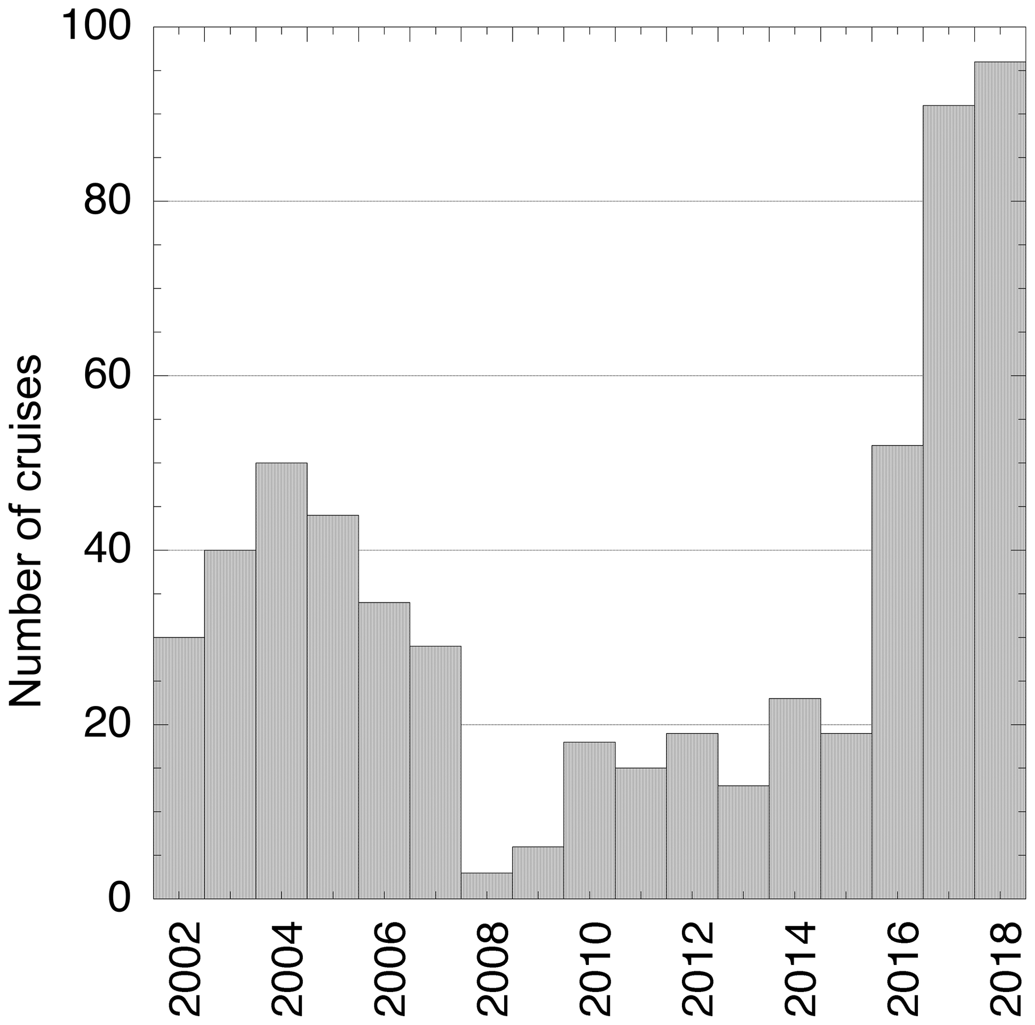
Over the past 20 years a rapidly expanding program of measurements of surface water partial pressure of carbon dioxide (pCO_2w)¹ or fugacity of CO₂ (fCO_2w)¹ has provided data to determine air–sea CO₂ fluxes and rates of ocean acidification on local to global scales (e.g., Boutin et al., 2008; Degrandpre et al., 2002; Evans et al., 2015; Schuster et al., 2013; Takahashi et al., 2014; Wanninkhof et al., 2019a, b). Marginal seas, which have historically had a dearth of measurements, have been targeted for increased observations. Through an industry, academic and federal partnership between the U.S. National Oceanic and Atmospheric Administration (NOAA), Royal Caribbean International (RCI) and the University of Miami, cruise ships were outfitted with automated surface water pCO₂ systems, also called underway pCO₂ systems (Pierrot et al., 2009). In 2002, the RCI ship Explorer of the Seas (EoS) was equipped with an underway pCO₂ setup providing observations on alternating weekly transects from Miami, FL, to the northeastern and northwestern Caribbean. In 2015, the EoS was repositioned out of the Atlantic, and the Celebrity Equinox (Eqnx) was outfitted with an underway pCO₂ system. Additionally, an underway pCO₂ system was installed on the Allure of the Seas (ALoS) in 2016. The Eqnx and ALoS covered similar transects as the EoS but on a more irregular and seasonal basis. A total of 582 cruises covered the region from 2002 through 2018. A map of all cruise tracks is shown in Fig. 1. The number of cruises per year covering the Caribbean Sea and adjacent western Atlantic is provided in Fig. 2. There are fewer cruises in the middle part of the record, when the EoS was diverted to other routes outside the area and eventually repositioned.

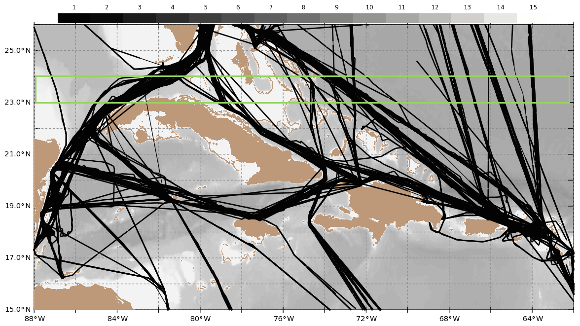
Figure 1 Map with the cruise tracks of the EoS, Eqnx and ALoS from 2002 though 2018. The gray scales show bathymetry, with white being less than 200 m. The green rectangle depicts the region where the data and products are compared in Fig. 4.

Figure 2 Histogram of number of cruises per year used in this work.

The surface water fCO₂ observational dataset and derived products including total alkalinity (TA), acidity (pH), aragonite saturation state (Ω_Ar) and air–sea CO₂ flux are of importance for determining the anthropogenic carbon uptake and to assess trends and impacts of ocean acidification. The observational data are provided to the global Surface Ocean CO₂ Atlas (SOCAT; Bakker et al., 2016) and global CO₂ climatology (Takahashi et al., 2009, 2018). These data are the main source of fCO₂ observations available in the region, and the high frequency of measurements provides a seasonally resolved picture of changing fCO_2w. This effort has made the northern Caribbean one of the few places in the world ocean where such regional observational density has been established. The data and mapped products are interpreted in Wanninkhof et al. (2019b), who show large decadal changes in trends of surface water fCO₂ and associated changes in air–sea CO₂ fluxes.

The data from the first part of this record form the basis of the ocean acidification product suite that maps ocean acidification conditions in the Caribbean (Gledhill et al., 2008; https://www.coral.noaa.gov/accrete/oaps.html, last access: 12 April 2020; https://cwcgom.aoml.noaa.gov/erddap/griddap/miamiacidification.graph, last access: 12 April 2020). The large, high-quality and well-resolved dataset is also used to validate models (Gomez et al., 2020).

For optimal application, datasets and associated data products are fully documented here and are readily accessible according to findable, accessible, interoperable and reusable (FAIR) principles (Wilkinson et al., 2016). In addition, the data underwent substantial quality control by our group and through the SOCAT quality control and check procedures. The documentation of the cruises, the sampling methodology and data reduction techniques are presented in brief. This is followed by a description of the approaches to calculate the different inorganic carbon system parameters. The procedure is to bin and average the fCO_2w on a 1^∘ by 1^∘ grid at monthly scales, referred to as gridded observations. Then the so-called second inorganic carbon system parameter is calculated. We estimate the total alkalinity (TA) based on robust relationships of TA with salinity (Cai et al., 2010; Takahashi et al., 2014; Lee et al., 2006; Millero et al., 1998) and use the software program CO2SYS (Pierrot et al., 2006) to calculate the other inorganic carbon system parameters of interest, in this case pH and Ω_Ar. These data products are presented at monthly scales binned and averaged on a 1^∘ by 1^∘ grid, referred to as gridded products. Annual multilinear regressions (MLRs) are developed between the gridded fCO_2w data and sea surface temperature (SST), sea surface salinity (SSS), location (latitude: lat; longitude: long) and mixed-layer depth (MLD) as independent variables. These regressions are applied at monthly and 1^∘ by 1^∘ spatial resolution to the region between 15 and 28^∘ N and between 88 and 62^∘ W using remotely sensed or modeled independent variables, and they are used to calculate air–sea CO₂ fluxes. These calculated parameters are called gridded mapped products. The procedures and datasets, including uncertainty analyses and tables of column headers of the product created, are provided below.

2 Observations

The observational program is described in terms of the ships, voyages and instrumentation. The ships predominantly sailed in the Caribbean Sea but also had tracks outside the region, including in the northeast of the USA as well as in Bermuda and in the Mediterranean. The description of operations, data and products presented here covers the northern Caribbean Sea and western Atlantic, north of the Caribbean island chain covering the region from 15 to 28^∘ N and −62 to −88^∘ (=62 to 88^∘ W; Fig. 1). The home ports of the ships, where passengers embark and disembark, are Miami and Fort Lauderdale, FL. The Explorer of the Seas (EoS) changed home port from Miami, FL, to Cape Liberty Cruise Port, NJ, in 2008 and changed its routes at that point to include cruises with Bermuda as a port of call. In 2015 the EoS was repositioned to the Pacific, and the underway pCO₂ system was removed. From 2015 onward the Celebrity Equinox (Eqnx) and from 2016 onward the Allure of the Seas (ALoS) covered the area. The Eqnx spent the summers of 2015 and 2016 in the Mediterranean, causing seasonal data gaps in the Caribbean.

2.1 Cruises

The EoS had 331 cruises from 2002 to 2015, the Eqnx completed 135 cruises from 2015 through 2018, and the ALoS performed 116 cruises in the study area from 2016 through 2018. Temporal coverage over the 17 years shows occupations every two weeks at the beginning of the record, from 2002 to 2007, and at the end, from 2014 through 2018, with fewer occupations in the years in between (Fig. 2). The cruises lasted between 7 and 14 d and made about a half a dozen ports of call. The ships were generally in port from early morning to late afternoon and transited between ports at night except for long runs (e.g., from Miami to San Juan), when the ship sailed continuously for several days. Ports are listed in the metadata accompanying the original data.

The systems were installed in different locations for the three ships, but each had a dedicated seawater intake near the bow. The EoS had an intake in the bow thruster tube (≈3 m depth) that was nonoptimal due to bubble entrainment during bow thruster operations and heavy seas. These observations have been culled from the datasets. The ALoS and Eqnx had their intake at ≈5 m depth, but it was forward from the bow thruster and had fewer issues with bubble entrainment. On the EoS, the underway pCO₂ instrument was initially in a dedicated science laboratory built for use on the ship and located amidships about 100 m from the intake. In 2008, a new system was placed in the engineering space closer to the bow with no apparent change in performance. For the ALoS and Eqnx, the instruments were near the bow intake in the engineering space, about 5 m from the intake. The EoS had an air intake mounted on a mast at the forward-most point of the main deck in August 2008. The Eqnx had an air intake near the bow, one level below the main deck, since the initial installation in March 2015. The underway pCO₂ systems on these ships made marine boundary layer (MBL) air observations (xCO_2a) as described in Wanninkhof et al. (2019b), but these are not used in the data products presented. Typical cruise speeds were 22 kn, which, with sampling every 2.5 min, yielded a fCO_2w sample approximately every 1.7 km except for 35 min every 4.5 h, when four calibration gases and a CO₂-free reference gas were analyzed, followed by five atmospheric CO₂ measurements for the ships with air intakes. This created a gap of 24 km ($\approx \mathrm{1}/\mathrm{4}$^∘) without fCO_2w measurements.

2.2 Instrumentation

2.2.1 pCO₂ system

The instrumentation is based on a community design described in Pierrot et al. (2009). The instruments were manufactured by General Oceanics Inc., and for the cruises described here they have performed to high-accuracy specifications. The surface water drawn from the intake at about 4 L min⁻¹ went through a 1.1 L spray head equilibrator with a water volume of 0.5 L and a headspace of 0.6 L. The spray and agitation caused the CO₂ in the headspace to equilibrate with the CO₂ in the water with a response time of about 2 min (Pierrot et al., 2009; Webb et al., 2016). Thus, the air in the headspace reached 99.8 % equilibration in 12 min. As the air is recirculated, and surface waters were relatively homogeneous on hourly timescales, 100.0 % equilibration was assumed. The four calibration gases supplied by the Global Monitoring Division (GMD) of the Environmental Science Research Laboratory (ESRL) of the NOAA were traceable to the WMO CO₂ mole fraction scale. The CO₂ concentrations of the standards spanned the range of surface water values encountered along the ship tracks (≈280–480 ppm).

The gas entering the analyzer was dried by passing it through a thermoelectric cooler at 5 ^∘C and a PermaPure drier. The standards did not contain water vapor. The air and equilibrator headspace analyses typically had about 10 % or less humidity. Every 27 h the CO₂ signal of the LI-COR model 6262 infrared analyzer was zeroed with the dry CO₂-free air and spanned with the highest standard. The water vapor channel was zeroed if it showed a reading of greater than 0.5 mmol mol⁻¹ for the dry CO₂-free air. The water vapor channel values are used for a minor correction to the xCO₂, and any inaccuracy in the H₂O results in <0.5 ppm change in the analyzer output of dry mole fraction of CO₂ (xCO₂ in parts per million, ppm). xCO₂ as calculated and output by the analyzer based on measured CO₂ and water vapor levels were recorded. The seawater circulation in the systems was automatically turned off when the ships entered port and back-flushed with fresh water, removing particles from the inline water filter and thereby alleviating clogging issues in the filter and reducing biofouling of water lines, the filter and the equilibrator.

Data from the ALoS and Eqnx were transmitted to shore daily and displayed online in graphical format at https://www.aoml.noaa.gov/ocd/ocdweb/allure/allure_realtime.html (last access: 30 June 2020) and https://www.aoml.noaa.gov/ocd/ocdweb/equinox/equinox_realtime.html (last access: 30 June 2020), respectively. These updates provided a near-real-time opportunity to look at the response of surface water CO₂ to episodic events, such as passage of hurricanes, and yielded timely indications of instrument malfunction that could be remedied by company engineers on board or when the ships returned to port. The instruments have shown agreement to within 1 µatm with other state-of-the-art systems in intercomparison studies (Yukihiro Nojiri, Ocean pCO₂ System Intercomparison at Hasaki, Japan, personal communication, February 2009). Several different versions of the instrument have been deployed on the ships over the years, but overall measurement principles and accuracies, estimated at better than 2 µatm (Pierrot et al., 2009; Wanninkhof et al., 2013), were maintained.

2.2.2 Thermosalinograph

Temperature and salinity were measured with a flow-through Sea-Bird SBE45 thermosalinograph (TSG) that was in a seawater flow line parallel to the pCO₂ equilibrator. A SBE38 remote temperature probe was situated near the inlet before the pump and was used as the SST measurement. The TSGs and temperature probes were maintained by collaborators from the Marine Technical group at the Rosenstiel School of Marine and Atmospheric Sciences (RSMAS) at the University of Miami (U. Miami). The TSGs on the ships were factory-calibrated on an annual basis. Postcalibrations showed no drift in the temperature sensor but occasionally some drift in the conductivity.

2.2.3 Other instrumentation

The underway effort is part of a larger scientific operation lead by RSMAS called Oceanscope (https://oceanscope.rsmas.miami.edu/, last access: 12 April 2020). Additional instrumentation on board the ships includes the Marine-Atmospheric Emitted Radiance Interferometer (M-AERI) to assess surface skin temperature retrievals from a number of radiometers on earth-observation satellites (Minnet et al., 2001). The M-AERIs are Fourier-transform infrared interferometers situated on the deck viewing the sea surface away from the wake. Acoustic Doppler current profilers (ADCPs) mounted on the hull of the ships are used to measure ocean currents.

3 Datasets

3.1 fCO₂ data

Full details on data acquisition with these systems and calculation of pCO₂ and fCO₂ can be found in Pierrot et al. (2009).

Postcruise, the xCO₂ data were processed by first linearly interpolating each standard measured every ∼4 h to the time of a sample measurement and then recalculating the air and water xCO₂ values based on the linear regression of the interpolated standard values at the time of sample measurement. For three cruises, the analyzer output showed negative water vapor values due to the condition of desiccant chemicals and thus yielded erroneous dry xCO₂ values. Separate processing routines were developed to correct for these situations (available on request from Denis Pierrot). The postcruise corrected xCO₂values were used for calculation of pCO₂ and fCO₂ as described in the calculation section.

3.2 Thermosalinograph, sea surface temperature and salinity data

The SST data were obtained from a temperature probe (Sea-Bird, model SBE38) near the intake. The salinity was determined with a thermosalinograph (Sea-Bird, model SBE45) from the measured conductivity and temperature in the unit using the internal software of the SBE45. The SST and SSS data were appended to the pCO₂ data records in real time and also logged via another shipboard computer at more frequent intervals. The SSS data were not quality-controlled, and no corrections to the SSS data were made other than the removal of spikes and values that were out of range (<5 and >40). As salinity has a minimal effect on the calculated fCO₂, bad or missing salinities were removed and substituted by linearly interpolated values to eliminate gaps. When SST data were not recorded in the CO₂ files and in the event of errors, the SST gaps were filled from the high-resolution SST data files maintained by the RSMAS Oceanscope project. On the rare occasion ($\approx <\mathrm{0.1}$ %) that SST was not recorded at all, SST data were estimated from the equilibrator temperature data (T_eq) after applying a constant offset between T_eq and SST using SST data before and after the gap. On average the T_eq was 0.12±0.28 ^∘C lower than SST for all the cruises. Per cruise the standard deviation (SD) of the difference of T_eq and SST was on the order of 0.04 ^∘C. The in situ fCO₂ data calculated with T_eq were flagged with a WOCE quality control flag of 3, which refers to data that are deemed questionable and have a larger uncertainty (https://www.nodc.noaa.gov/woce/woce_v3/wocedata_1/whp/exchange/exchange_format_desc.htm, last access: 12 April 2020).

For the regionally mapped products on a 1^∘ grid and monthly timescale (1^∘ by 1^∘ by month), SST and SSS were obtained from the following sources: the SSS data were from a numerical model, the Hybrid Coordinate Ocean Model (HYCOM; https://HYCOM.org/, last access: 12 April 2020), and are referred to as SSS_HYCOM. The SST product for the region was the optimum interpolated SST (OISST) from https://www.esrl.noaa.gov/psd/ (last access: 12 April 2020) (Reynolds et al., 2007). It uses data from ships, buoys and satellites to generate the fields. For the OISST the reference SST is from buoys, and the other SST data obtained from ships and other platforms were adjusted to the buoy data by subtracting 0.14 ^∘C in the OISST product (Reynolds et al., 2007).

3.3 Wind speed data

Winds were measured on the ships, but these data are not used as they are not synoptic for the whole region, which is a requirement for the regional flux maps. Instead, wind speeds were obtained from the updated cross-calibrated multiplatform wind product (CCMP-2; Atlas et al., 2011). The mean scalar neutral wind at 10 m height $<u_{\mathrm{10}}>$ and its second moment $<u_{\mathrm{10}}^{\mathrm{2}}>$ were used to calculate the fluxes. They were determined from the 1∕4^∘, 6-hourly product that was obtained from remote-sensing systems (RSSs; http://www.remss.com/, last access: 6 June 2020). This product relies heavily on the European Centre for Medium-Range Weather Forecasts (ECMWF) assimilation scheme that uses in situ and remotely sensed assets, particularly (passive) radiometers on satellites. The directional component uses scatterometer data. The 1∕4^∘, 6-hourly CCMP-2 product was binned and averaged in 1^∘ grid boxes at monthly scales (1^∘ by 1^∘ by month). In the absence of CCMP-2 data for 2018, the wind product from European Reanalysis, ERA5, was used (https://www.ecmwf.int/en/forecasts/datasets/reanalysis-datasets/era5, last access: 6 June 2020. Copernicus Climate Change Service, 2017). The ERA5 wind data are at 31 km and 3-hourly resolution but were binned and averaged in the same manner as the CCMP-2 winds. There were no apparent biases between the scalar winds for the two products in the Caribbean.

3.4 Mixed-layer depth data

No MLD determinations were made on the cruises, and limited observational estimates from other sources are available. The MLDs provided here are from the same numerical model (HYCOM) as used for the mapped SSS and obtained from http://www.science.oregonstate.edu/ocean.productivity/index.php (last access: 12 April 2020). The MLDs are based on a density contrast of 0.03 between surface and subsurface. MLDs are used as an independent variable in the MLRs to map the fCO_2w values. They are also needed if mixed-layer dissolved inorganic carbon (DIC) inventories are desired and to determine the effect of mixed-layer depth on the changes in fCO_2w. As shown in Wanninkhof et al. (2019b, Fig. 9), MLDs are negatively correlated with fCO_2w. They are provided in the gridded mapped product.

4 Calculations

The calculations of the concentrations and fluxes follow standard procedures as described below. The mapping procedures are detailed. The section on uncertainty includes an example of different possible means of mapping and the effect on the final product.

4.1 Calculation of pCO₂

The starting point in the calculations, which were aided by the use of MATLAB routines following the procedures as in Pierrot et al. (2009), was calibrated (dry) xCO₂ values.

The xCO₂ values were converted to pCO_2eq (µatm) values:

$$\begin{array}{}\text{(1)}& p{\mathrm{CO}}_{\mathrm{2}\mathrm{eq}}={\mathrm{xCO}}_{\mathrm{2}\mathrm{eq}}(P_{\mathrm{eq}}-{\mathrm{pH}}_{\mathrm{2}}\mathrm{O}),\end{array}$$

where eq refers to equilibrator conditions. P_eq is the pressure in the equilibrator headspace, and pH₂O is the water vapor pressure calculated according to Eq. (10) in Weiss and Price (1980). The pCO_2eq was corrected to surface water values using the intake temperature (SST) and the temperature of water in the equilibrator (T_eq) according to the empirical relationship that Takahashi et al. (1993) developed for North Atlantic surface waters:

$$\begin{array}{}\text{(2)}& p{\mathrm{CO}}_{\mathrm{2}\mathrm{w}}=p{\mathrm{CO}}_{\mathrm{2}\mathrm{eq}}{e}^{\left(\mathrm{0.0423}\right(\text{SST}-T_{\mathrm{eq}}\left)\right)}.\end{array}$$

This empirical correction for temperature is widely used, but it is of note that applying the thermodynamic relationships for carbonate dissociation constants yields different temperature dependencies that are a function of temperature. For the average SST in the Caribbean of 27.0 ^∘C the coefficient of temperature dependence varies from 0.036 to 0.040 using commonly used constants as provided in inorganic carbon system programs such as CO2SYS (Pierrot et al., 2006) compared to the coefficient of 0.0423 (or 4.23 % ^∘C⁻¹) used above. On average the difference between SST and T_eq is 0.12 ^∘C for all the cruises such that the correction from T_eq to SST using the coefficient of 0.0423 in Eq. (2) is 1.9 µatm under average conditions of SST =27 ^∘C and pCO_2w =374 µatm. Using a temperature coefficient of 0.036 the temperature correction would be 1.6 µatm, or a 0.3 µatm difference.

4.2 Calculation of fCO₂ in air and water

The fCO₂ is the pCO₂ corrected for nonideality of CO₂ solubility in water using the virial equation of state (Weiss, 1974). The correction can be expressed as fCO_2a,w = e^g(SST,P) pCO_2a,w and

$$\begin{array}{}\text{(3)}& \begin{array}{rl}g(T,P)=& \left[\right(-\mathrm{1636.75}+\mathrm{12.0408}T-\mathrm{0.0327957}{T}^{\mathrm{2}}\\ & +\mathrm{0.0000316528}{T}^{\mathrm{3}})+\mathrm{2}(\mathrm{1}-{\mathrm{xCO}}_{\mathrm{2}}{\mathrm{10}}^{-\mathrm{6}}{)}^{\mathrm{2}}\\ & (\mathrm{57.7}-\mathrm{0.118}T)(P/\mathrm{1013.25})]/(\mathrm{82.0575}T)\end{array},\end{array}$$

where T is in kelvin, xCO₂ is in parts per million, and P is in millibars.

Under average conditions in the Caribbean, the function $e^{g(\mathrm{SST},P)}\approx \mathrm{0.997}$ and fCO_2w will be ≈1.2 µatm less than pCO_2w. As the corrections from partial pressure to fugacity in air and water are approximately the same, the difference between ΔpCO₂ (= pCO_2w-pCO_2a) and ΔfCO₂ (= fCO_2w-fCO_2a), which were used to determine the fluxes (Eq. 5), is negligible ($\approx <\mathrm{0.1}$ µatm).

4.3 Gridding procedure

Gridding of the observations of fCO_2w, SST and SSS was performed by binning and averaging the data in (1^∘ by 1^∘ by month) cells. At typical ship speeds of 22 kn, the ship covered 1^∘ in about 2.5 h, taking 60 measurements. This would yield about 250 measurements per month assuming weekly cruises through the area. The actual number of measurements per grid cell ranged from 8 to 500. The higher number of observations per cell was mostly in the latter part of the record, when the Eqnx and ALoS operated in the same area. The total number of observations from March 2002 through December 2018 was 1.13 million, and the total number of (1^∘ by 1^∘ by month) grid cells with observations was 9224.

The gridding facilitated the colocation and merging of products such as MLD_HYCOM, SSS_HYCOM, OISST, $<u^{\mathrm{2}}{>}_{\mathrm{CCMP}}$ and marine boundary layer xCO₂ (xCO_2aMBL) into the gridded observational dataset for further interpretation. The gridded data aided comparison of in situ SST with OISST and SSS with SSS_HYCOM. The average difference between SSS and SSS_HYCOM for the 2002–2018 data was $-\mathrm{0.1}\pm \mathrm{0.28}$ (n=9224), and for SST and OISST the difference was 0.25±0.40 ^∘C (n=9224), with the in situ SSS being lower and SST being higher. While both differences include zero within their standard deviation, the temperature difference is in agreement with expected cooler near-surface temperatures that could lead to lower fCO_2w values, which in turn have a large impact on the calculated air–sea fluxes.

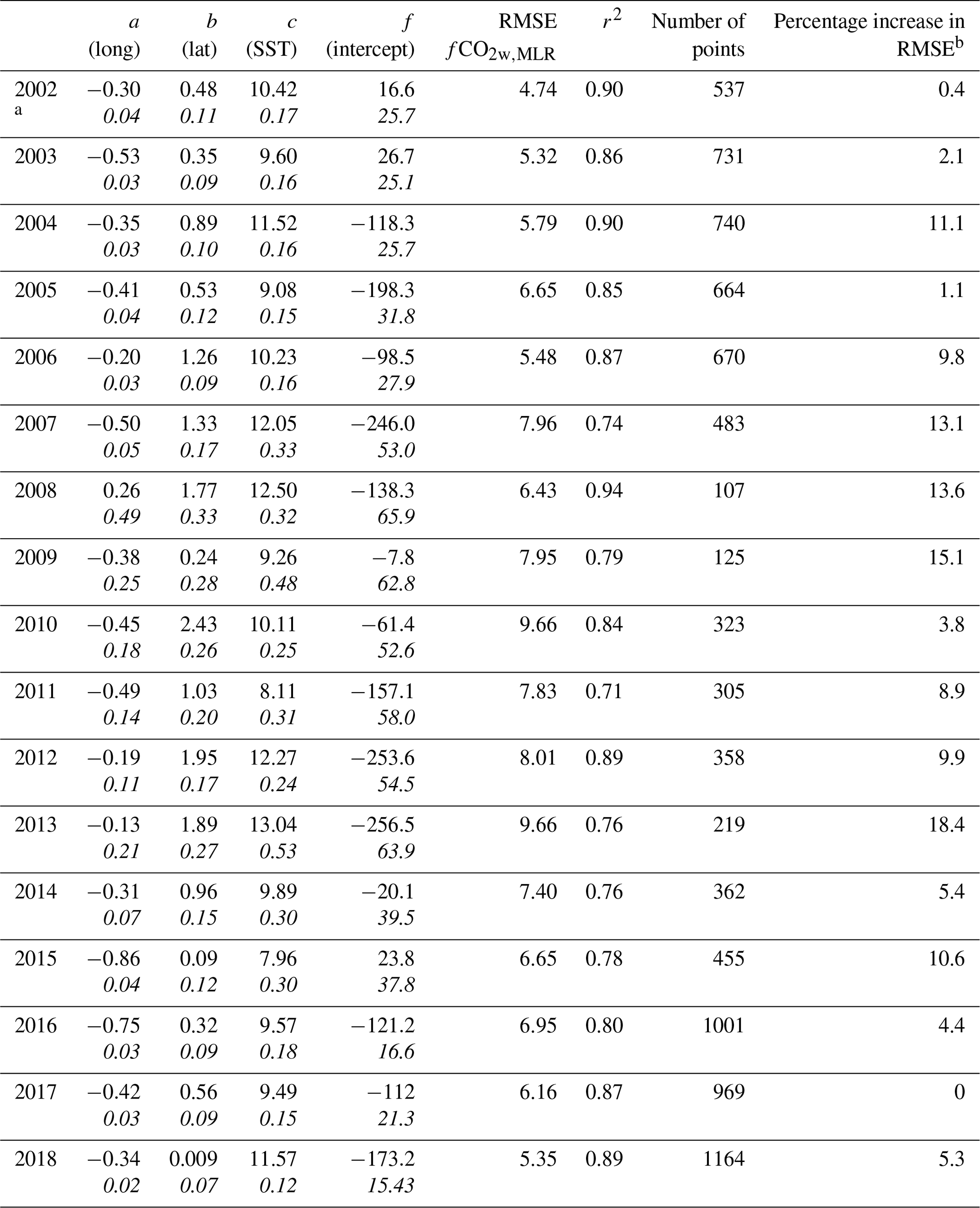
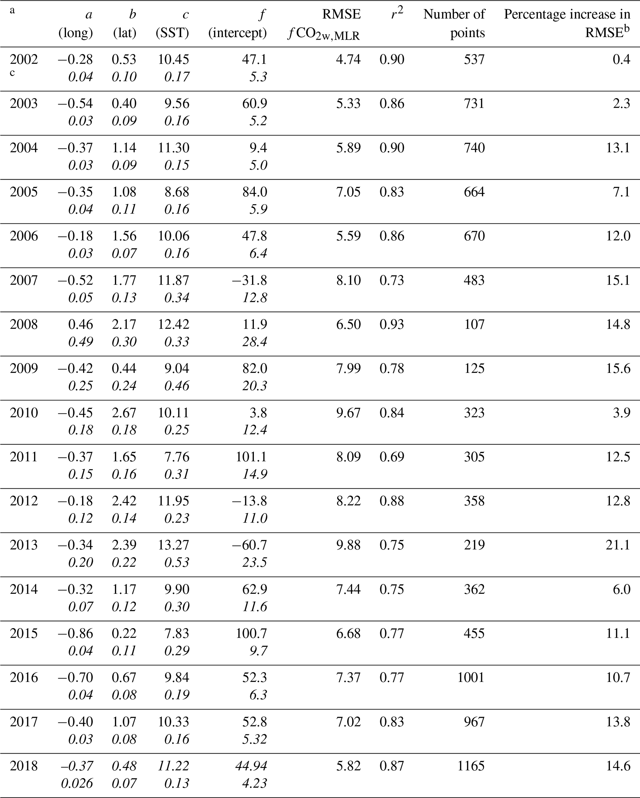
Table 1 Coefficients for the MLR for each year^*.

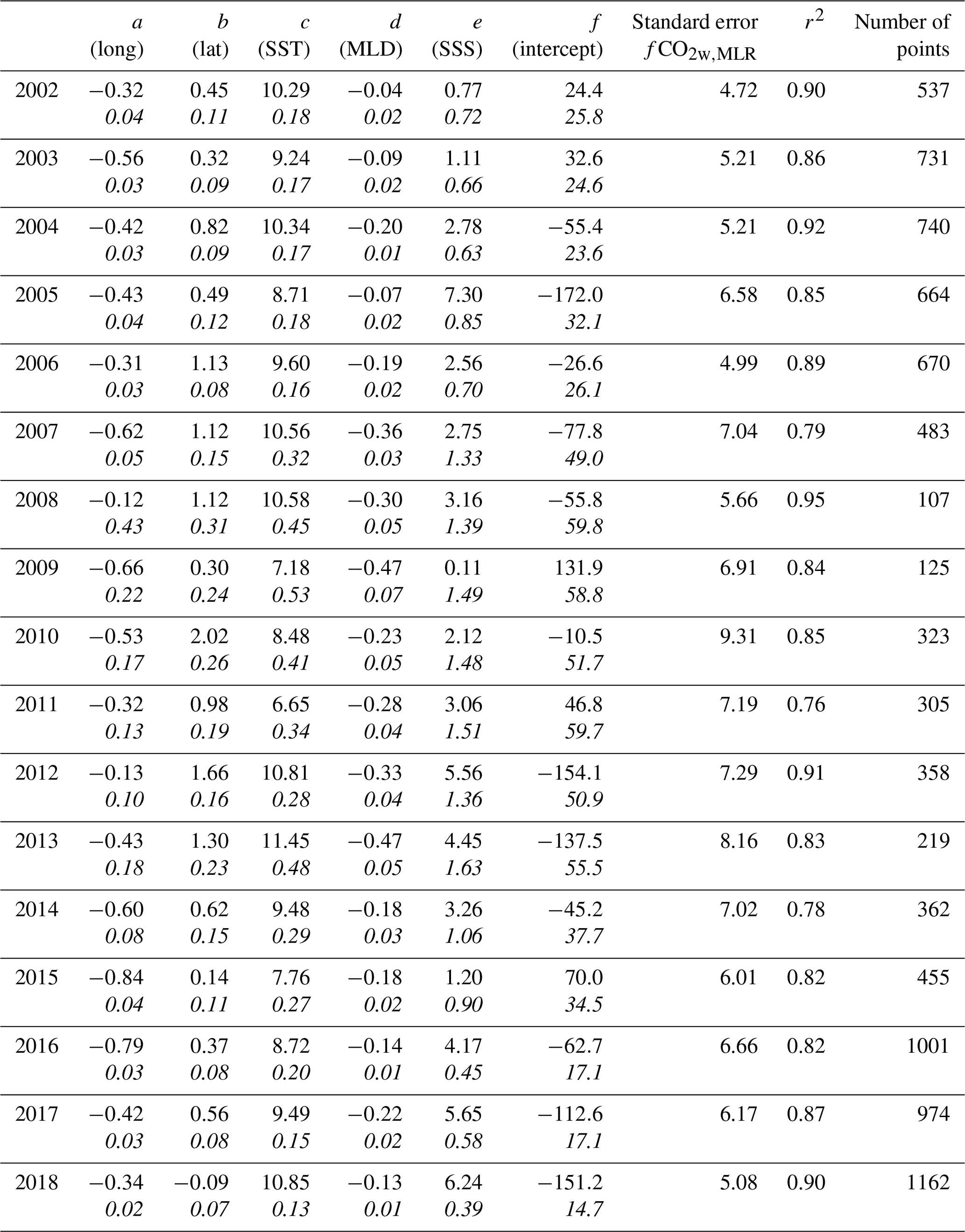
^* These annual regressions were used to create the mapped fCO_2wMLR fields using the 1^∘ by 1^∘ by month gridded data product. fCO_2wMLR = a longitude + b latitude + c OISST + d MLD_HYCOM + e SSS_HYCOM+f. The second row (in italics) for each annual entry is the error of the coefficient.

4.4 Mapping procedures for fCO_2w and fluxes

4.4.1 Mapping fCO_2w using a multilinear regression

The gridded observations (1^∘ by 1^∘ by month) represented about 10 % of the area and months of investigation from 15 to 28^∘ N and 88 to 62^∘ W over the period of investigation. To interpolate (“map”) the data in space (334 grid cells) and time (192 months) a multilinear regression (MLR) approach was used to determine fCO_2w in each grid cell. For each year from 2002 through 2018 the gridded fCO_2w observations were regressed against the 1^∘ monthly gridded values of position (lat and long), SST, MLD and SSS. Other permutations of independent parameters were tested but yielded less robust fits (see Appendix A). Annual MLRs were created as fCO_2w levels change over time in response to increasing atmospheric CO₂ levels. If fCO_2w kept pace with atmospheric CO₂ increase, this would translate to a linear trend of fCO_2w of 2.13 µatm yr⁻¹ over the time period. As shown in Wanninkhof et al. (2019b), multiyear (>4-year intervals) trends varied from −4 to 4 µatm yr⁻¹, with an average linear trend in fCO_2w of 1.4 µatm yr⁻¹ from 2002 to 2018.

The annual MLRs were created of the form

$$\begin{array}{}\text{(4)}& \begin{array}{rl}f{\mathrm{CO}}_{\mathrm{2}\mathrm{w}}=& a\mathrm{lon}+b\mathrm{lat}+c\mathrm{OISST}+d{\mathrm{MLD}}_{\mathrm{HYCOM}}\\ & +e{\mathrm{SSS}}_{\mathrm{HYCOM}}+f,\end{array}\end{array}$$

with the coefficients for each year along with the standard error in fCO_2w and standard error in each of the coefficients provided in Table 1. The standard error in the fCO_2wMLR ranged from 5 to 9 µatm for each year. Using the locations, OISST (the optimal interpolated SST product), MLD_HYCOM and the SSS_HYCOM (output of the HYCOM model) the fCO_2wMLR are determined for each grid cell. There were significant cross-correlations between independent variables such that the effect of the often significant year-to-year differences in coefficients was difficult to interpret. However, the fCO_2wMLR from the annual MLRs faithfully reproduced the trends and variability.

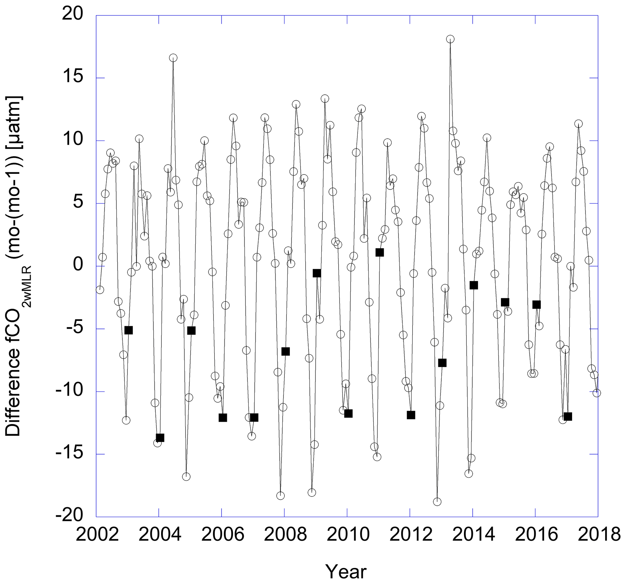
Figure 3 The difference between fCO_2wMLR for subsequent months plotted versus time. The solid squares are the differences between December and January where different MLRs are used.

The MLRs were produced for each year such that the mapped products could be extended for future years in a straightforward fashion. To determine if there were anomalous discontinuities between subsequent annual MLRs that could impact the time series, the difference between fCO_2w for subsequent months was plotted versus time in Fig. 3. No significant discontinuities were observed between December and January. Only for December and January 2008/2009, 2009/2010 and 2016/2017 do there appear to be slight differences in the pattern of monthly progressions, but such anomalies are observed during other times of year as well. Using an MLR that includes year as one of the coefficients (see Appendix A, Eqs. A3 and A4) provides a slightly worse fit. Moreover, using such a fit would necessitate recalculating the mapped products every time a new year is added.

To illustrate the differences between gridded and mapped products, the results of the fCO_2wMLR calculated with the MLRs for 2004, 2011 and 2017 (Table 1) are plotted in Fig. 4a along with the gridded observations for the grid cells that span the longitude range from 88 to 62^∘ W between 23 and 24^∘ N (see Fig. 1). Figure 4a shows that the mapped product using annual MLRs shows the increases in fCO_2w over time in the region and consistent differences in patterns between the east and the west for the 3 years. The mapped product showed a reasonable correspondence with the gridded observations. Some of the differences between the gridded observations and mapped product were caused by the mismatch between SST and SSS in situ with the OISST and SSS_HYCOM (Fig. 4b and c). In particular, the strong minima in OISST at 79^∘ W are not seen in the SST. This is likely because the OISST captured the lower SST near the coast of Cuba. This caused the fCO_2wMLR product to be lower as well, as shown in Fig. 4a. It illustrates that the mapped fCO_2wMLR product is influenced by both the annual MLR and the gridded MLD_HYCOM, OISST and SSS_HYCOM.

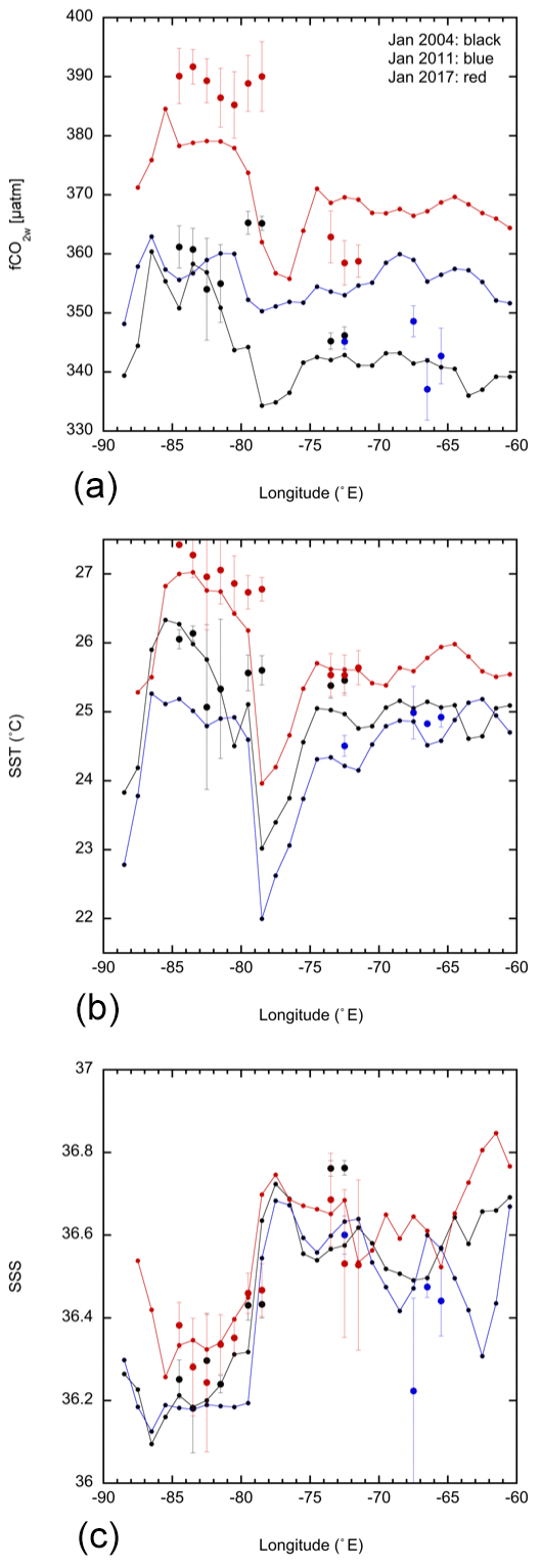
Figure 4 Zonal section of gridded and mapped products between 23 and 24^∘ N for January 2004 (black), January 2011 (blue) and January 2017 (red). (a) fCO_2w; (b) SST; (c) SSS. The lines with small solid circles are the mapped product; the larger solid circles are the gridded data, with standard deviation of data in the box shown as error bars.

4.4.2 Determining the air–sea CO₂ fluxes for the region

For the determination of the air–sea CO₂ flux ($F_{{\mathrm{CO}}_{\mathrm{2}}}$, mol m⁻² yr⁻¹), a bulk formulation was applied using the gridded mapped product

$$\begin{array}{}\text{(5)}& F_{{\mathrm{CO}}_{\mathrm{2}}}=k{K}_{\mathrm{0}}\mathrm{\Delta }f{\mathrm{CO}}_{\mathrm{2}},\end{array}$$

where ΔfCO₂ is (fCO_2w-fCO_2a), K₀ is the seawater CO₂ solubility that is a function of temperature and salinity (Weiss and Price, 1980), and k is the gas transfer velocity parameterized as a function of wind speed (Wanninkhof, 2014).

$$\begin{array}{}\text{(6)}& k=\mathrm{0.251}<u_{\mathrm{10}}^{\mathrm{2}}>(Sc/\mathrm{660}{)}^{-\mathrm{1}/\mathrm{2}},\end{array}$$

where $<u_{\mathrm{10}}^{\mathrm{2}}>$ is the monthly second moment of the wind speeds reported in CCMP-2. The second moment accounts for the impact of variability of the wind speed on k. It is determined by taking the monthly average of the sum of squares of the wind speed in CCMP-2 provided at 6 h and 1∕4^∘ grid resolution. The number of wind speed observations in a (1^∘ by 1^∘ by month) grid is 1920. This sample density captures the frequency spectrum of winds in the grid boxes except that extreme wind events such as hurricanes are not fully represented due to the local nature of the extremes and inherent smoothing in the CCMP-2 product. Sc is the Schmidt number of CO₂ in seawater, defined as the kinematic viscosity of seawater divided by the molecular diffusion coefficient of CO₂. It is determined as a function of temperature from Wanninkhof (2014). At the average temperature of 27 ^∘C the $S{c}_{{\mathrm{CO}}_{\mathrm{2}}}$ equals 475. Over the typical range of SST in the Caribbean from 24 to 30 ^∘C, the (Sc∕660)${}^{-\mathrm{1}/\mathrm{2}}$ will vary from 1.1 to 1.27, indicating that the gas transfer velocity will be 27 % higher at an SST of 30 ^∘C compared to an SST of 20 ^∘C that would correspond to an Sc of 660.

The annual fCO_2wMLR values as well as the modeled and remotely sensed products OISST, MLD_HYCOM and SSS_HYCOM were determined for all (1^∘ by 1^∘ by month) grid cells. The monthly fCO_2aMBL values were derived from the weekly average xCO_2aMBL of the stations on Key Biscayne (KEY) and Ragged Point Barbados (RPB; CarbonTracker Team, 2019; https://www.esrl.noaa.gov/gmd/ccgg/flask.php, last access: 20 June 2020). The second moments of the scalar winds $<u^{\mathrm{2}}>$ from CCMP-2 were averaged on the same grids. As no CCMP-2 product was available in 2018, the ERA5 wind product was used for the last year of the record.

4.5 Gridded and mapped products for alkalinity and pH_T

Total alkalinity (TA) was determined from salinity. For estimation of TA, several algorithms have been developed with salinity (Fig. 5; Millero et al., 1998; Lee et al., 2006; Takahashi et al., 2014 and Cai et al., 2010). The relationship of Cai et al. (2010), TA =57.3 SSS +296.4, SD =5.5, was used as this was determined from observations that are similar to the conditions in the Caribbean.

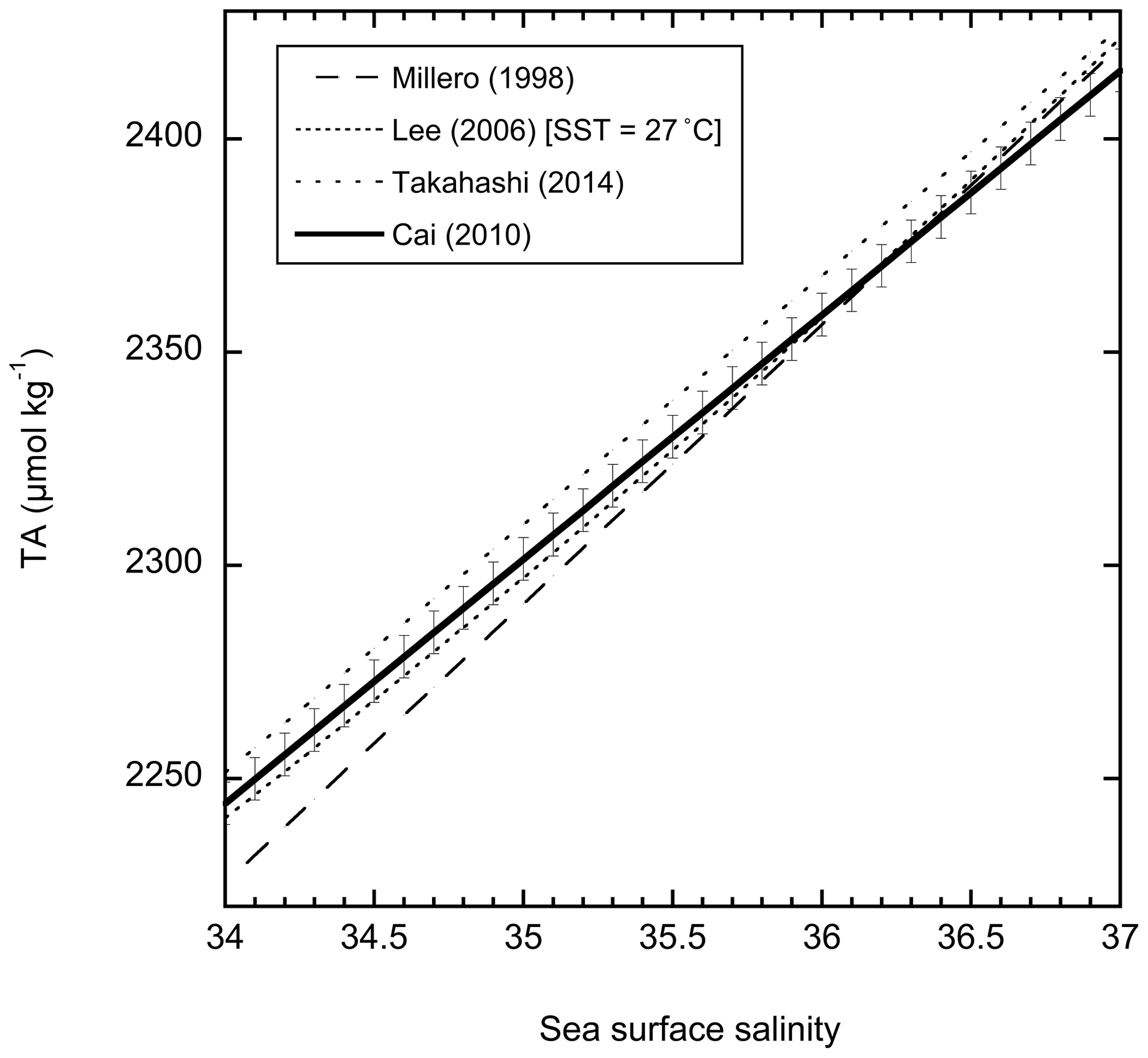
Figure 5 Relationships of surface water TA with salinity. The relationship of Cai et al. (2010), with standard error shown as error bars, is used to calculate pH and Ω_Ar from fCO_2w.

The pH_T, the pH on the total scale at SST, was subsequently determined from the calculated TA and fCO_2w. For the gridded products the gridded SSS was used to determine TA. For the pH_T the gridded TA, SST and fCO_2w were used. For the mapped products the gridded OISST and SSS_Hycom were applied in the calculations. The pH_T was calculated using the program CO2SYS for Excel V2.2 (Pierrot et al., 2006) with the apparent CO₂ dissociation constants K₁ and K₂ from Lueker et al. (2000), the ${\mathrm{KSO}}_{\mathrm{4}}^{-}$ dissociation constant from Dickson (1990), the KF dissociation constant from Perez and Fraga (1987), and the total boron relationship with salinity from Uppström (1974).

Table 2 Estimated uncertainties in measured, gridded and mapped variables.

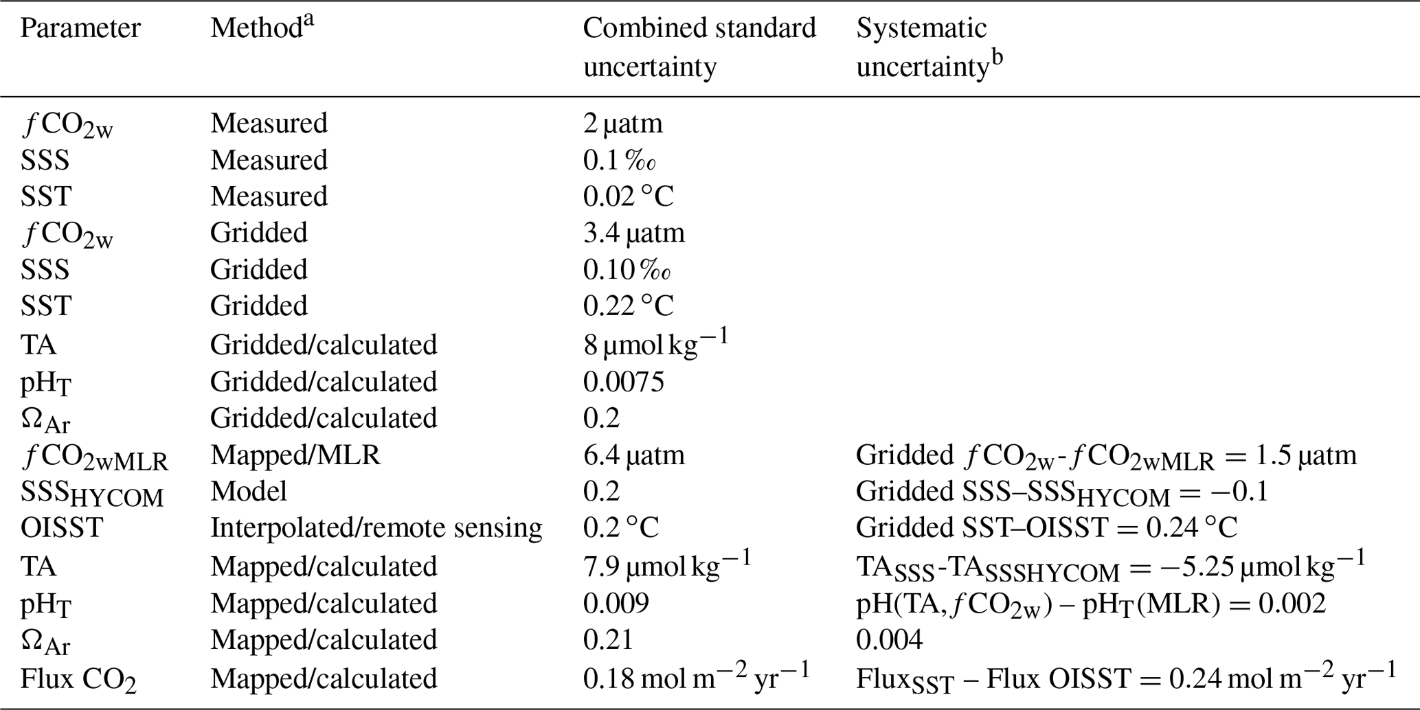
^a Method refers to either the individual data point (measured), the values averaged on a 1^∘ by 1^∘ by month grid, or the interpolated products (mapped). ^b The systematic uncertainty is based on the difference between the different methods and products as indicated. Note that the combined standard uncertainties and systematic uncertainties are based on average conditions.

Table 3 Column headers, units and description for the monthly 1^∘ gridded observational product (1^∘ by 1^∘ by month).

4.6 Aragonite saturation state (Ω_Ar)

The aragonite saturation state (Ω_Ar) indicates the level of supersaturation or undersaturation of seawater with respect to the mineral aragonite, a polymorph of calcium carbonate, and part of the skeletal structure of many marine calcifiers. When Ω_Ar is less than 1, aragonite dissolution is thermodynamically favored, and when Ω_Ar is greater than 1, it has a tendency to precipitate. The Ω_Ar is used as an indicator of ecosystem health with regards to ocean acidification (Mollica et al., 2018). In warm tropical regions surface water saturation states are well above 1, but no active precipitation takes place except under unusual circumstances in shallow waters, in a precipitation process called whitings (Purkis et al., 2017). The Ω_Ar is not measured directly and is defined as the product of calcium and carbonate ion concentrations divided by the solubility product of aragonite:

$$\begin{array}{}\text{(7)}& {\mathrm{\Omega }}_{\mathrm{Ar}}=\left[{\mathrm{Ca}}^{\mathrm{2}+}\right]\left[{\mathrm{CO}}_{\mathrm{3}}^{\mathrm{2}-}\right]{\left(K_{\mathrm{Ar}}{\prime }_{\mathrm{sp}}\right)}^{-\mathrm{1}},\end{array}$$

where $\left[{\mathrm{Ca}}^{\mathrm{2}+}\right]=\mathrm{0.02128}/\mathrm{40.087}\times (\mathrm{SSS}/\mathrm{1.80655})=\mathrm{293.84}$ SSS (in moles per kilogram of seawater) is the total calcium concentration, derived from salinity (Riley and Tongudai, 1967). $\left[{\mathrm{CO}}_{\mathrm{3}}^{\mathrm{2}-}\right]$ is the total carbonate ion concentration determined from two of the inorganic carbon system parameters, and K_Ar′_sp is the apparent solubility product of aragonite in seawater at a specified salinity, temperature and pressure. In this work $\left[{\mathrm{CO}}_{\mathrm{3}}^{\mathrm{2}-}\right]$ is determined from the gridded fCO_2w and calculated TA using the CO2SYS program. For surface waters, K_Ar′_sp is

$$\begin{array}{}\text{(8)}& \begin{array}{rl}p{K}_{\mathrm{Ar}}{\prime }_{\mathrm{sp}}=& -[-\mathrm{171.945}-\mathrm{0.077993}T+\mathrm{2903.293}/T\\ & +\mathrm{71.595}\log \left(T\right)+(-\mathrm{0.068393}\\ & +\mathrm{0.0017276}T+\mathrm{88.135}/T)S^{\mathrm{0.5}}\\ & -\mathrm{0.10018}S+\mathrm{0.0059415}{S}^{\mathrm{1.5}}],\end{array}\end{array}$$

where $p{K}_{\mathrm{Ar}}{\prime }_{\mathrm{sp}}=-\log K_{\mathrm{Ar}}{\prime }_{\mathrm{sp}}$, T is temperature in kelvin (K) and S is salinity (Mucci, 1983). As with pH_T, the Ω_Ar-gridded product was determined from the gridded (1^∘ by 1^∘ by month) values of SSS, SST, fCO_2w and TA, while the mapped product uses SSS_HYCOM, OISST, fCO_2wMLR and TA.

4.7 Uncertainty of observations and the gridded and mapped products

The uncertainty of the products is difficult to quantify due to the many factors, calculations and interpolations influencing the overall uncertainty. Moreover, the uncertainty estimate includes a random and a systematic component. The latter can have a large influence on interpretations, particularly on the calculated air–sea CO₂ fluxes. Below we address the uncertainty in terms of standard errors in the observations, in the gridded products and in the mapped products. For the calculated quantities and nomenclature we follow the approach in Orr et al. (2018). The standard uncertainty is characterized by its standard deviation or error of the measured quantities and the standard uncertainties of the input variables. The propagated uncertainty of a calculated variable is called the combined standard uncertainty. Error propagation is ($e_A^{\mathrm{2}}+e_B^{\mathrm{2}}+\mathrm{\dots }{)}^{\mathrm{0.5}}$ for addition and $\left(\right(e_A/A{)}^{\mathrm{2}}+(e_B/B{)}^{\mathrm{2}}+\mathrm{\dots }{)}^{\mathrm{0.5}}$ for multiplication, where A and B are the variables, and e_A is the standard error in variable A.

The individual measurements of fCO_2w have a combined standard uncertainty of less than 2 µatm based on a propagation of error of instrument response, equilibrator efficiency standardization, and temperatures and pressures at equilibration and at the sea surface (Pierrot et al., 2006). The performance and output data from the UWpCO₂ systems have been checked by the manufacturer, in intercomparison exercises and at sea. At the point of measurement, SST measurements are accurate to 0.02 ^∘C and SSS measurements to 0.1 based on instrument specifications and annual calibrations.

The combined standard uncertainty in the gridded product will vary based on the number of measurements. It includes the actual variability in the 1^∘ by 1^∘ cells. To estimate the uncertainty per grid cell, the standard deviation of the fCO_2w in each cell was determined, and then the average of the standard deviations for the 9924 cells with observations was taken. The average standard deviation was 3.4±2.6 µatm (n=9224). The same procedure was followed for SST and SSS and yielded values of 0.22±0.19 ^∘C for SST and 0.10±0.10 for SSS. These were relatively small uncertainties compared to the monthly spatial range of ≈20 µatm for fCO_2w, ≈1 ^∘C for SST and ≈1 for SSS. The amplitudes of the seasonal cycle of ≈40 µatm for fCO_2w and ≈4 ^∘C for SST were significantly greater than the standard uncertainties as well.

The calculated parameters for the gridded products, TA, pH_T and Ω_Ar have an added uncertainty due to the uncertainty in the constants and parameterizations. The agreement between the TA–SSS relationships was good, and choice of TA relationship did not have a determining influence on results. We used TA =57.3 SSS_OBS +296.4 specifically developed for the subtropical western Atlantic (see insert of Fig. 10 in Cai et al., 2010). The standard error for the relationship was 5.5 µmol kg⁻¹. The average standard deviation for salinity in the grid cells is 0.1, which translates to an uncertainty in gridded TA of 5.7 µmol kg⁻¹. Thus the combined standard uncertainty for TA is ${\left({\left(\mathrm{5.5}\right)}^{\mathrm{2}}+{\left(\mathrm{5.7}\right)}^{\mathrm{2}}\right)}^{\mathrm{0.5}}=\mathrm{7.9}$ µmol kg⁻¹.

pH_T is determined from fCO_2w and calculated TA with associated uncertainties. An added uncertainty for the calculated pH_T is the uncertainty in the dissociation constants that are used to calculate pH_T. These uncertainties can be calculated using a modified version of CO2SYS (Orr et al., 2018). As shown in Orr et al. (2018, Fig. 12), the uncertainty in the constants dominates the calculated pH_T. Using the uncertainty in the constants as presented in the program, an uncertainty of gridded TA of 8 µmol kg⁻¹ and 3.4 µatm for fCO₂ yields a combined standard uncertainty in pH of 0.0075. For comparison, the uncertainty in pH would be 0.0070 if state-of-the-art measurement uncertainties in TA of ±3 µmol kg⁻¹ and ±2 µatm for fCO₂ are used. Similarly, the uncertainty of Ω_Arusing the same approach and uncertainties in independent parameters are ±0.20. Again it is the uncertainty in the dissociation constants that dominate the overall uncertainty.

For the mapped products there is additional uncertainty due to the use of regressions. The standard errors of the annual regressions in fCO_2wMLR and the coefficients of the independent parameters are provided in Table 1. The average standard error for the fCO_2wMLR for the 17 years is 6.4±1.2 µatm. Following the approach above for the other independent parameters and propagating these uncertainties yields a combined standard uncertainty of 0.0090 in mapped pH and 0.21 in mapped Ω_Ar.

Systematic errors are introduced by the different SST and SSS data that are used for the gridded and mapped products, with the former using the gridded measured SST and SSS and the latter using the SSS_HYCOM and OISST products. The magnitude of the systematic uncertainty between the mapped and gridded product is estimated from the difference in the gridded and mapped parameters for cells that have both gridded and mapped products (for columns headers, see Table 2). Another possible source of systematic uncertainty is using the gridded and mapped fCO_2sw, SSS and SST to calculate the TA, pH_T and Ω_Ar rather than using the in situ values to calculate the parameters and then gridding them. This uncertainty is small based on the low uncertainty of variables in each cell as shown from their standard deviations provided in the gridded products (for column headers, see Table 3).

This is confirmed by comparing this method with the approach of calculating the pH and then gridding and mapping as done in Lauvset et al. (2016) and Jiang et al. (2015). To examine the differences derived from using one or the other approach, both were compared for 2017 data. The pH and TA were calculated for every fCO_2w observation and binned into a ($\mathrm{1}{}^{\circ }\times \mathrm{1}{}^{\circ }\times$ mo) grid. An MLR from the calculated pH was created for 2017:

$$\begin{array}{}\text{(9)}& \begin{array}{rl}{\mathrm{pH}}_{\mathrm{T}}(\pm \mathrm{0.005})=& \mathrm{0.0003194}\mathrm{long}-\mathrm{0.00046744}\mathrm{lat}\\ & -\mathrm{0.00965183}\mathrm{SST}+\mathrm{0.00019602}\mathrm{MLD}\\ & +\mathrm{0.00069378}\mathrm{SSS}+\mathrm{8.3240},r^{\mathrm{2}}\\ & =\mathrm{0.89}(n=\mathrm{1244}).\end{array}\end{array}$$

This MLR was then applied to the independent variables for each grid box to determine pH_T(MLR). This was compared to the approach used here of calculating the pH using the mapped fCO_2wMLRand TA–SSS relationships on ($\mathrm{1}{}^{\circ }\times \mathrm{1}{}^{\circ }\times$ mo) grids, called pH_T(fCO_2w,TA). The two approaches provided similar results, with pH_T(fCO_2w,TA) – pH_T(MLR) $=-\mathrm{0.0001}\pm \mathrm{0.005}$ for 2017. The small difference showed a pattern with SST (Fig. 6) but not with the other independent variables. The differences using either pH_T(fCO_2w,TA) or pH_T,MLR are an order of magnitude smaller than the combined standard uncertainties such that the approach of using mapped fCO_2w and TA to determine pH_T yielded precise and consistent gridded pH_T.

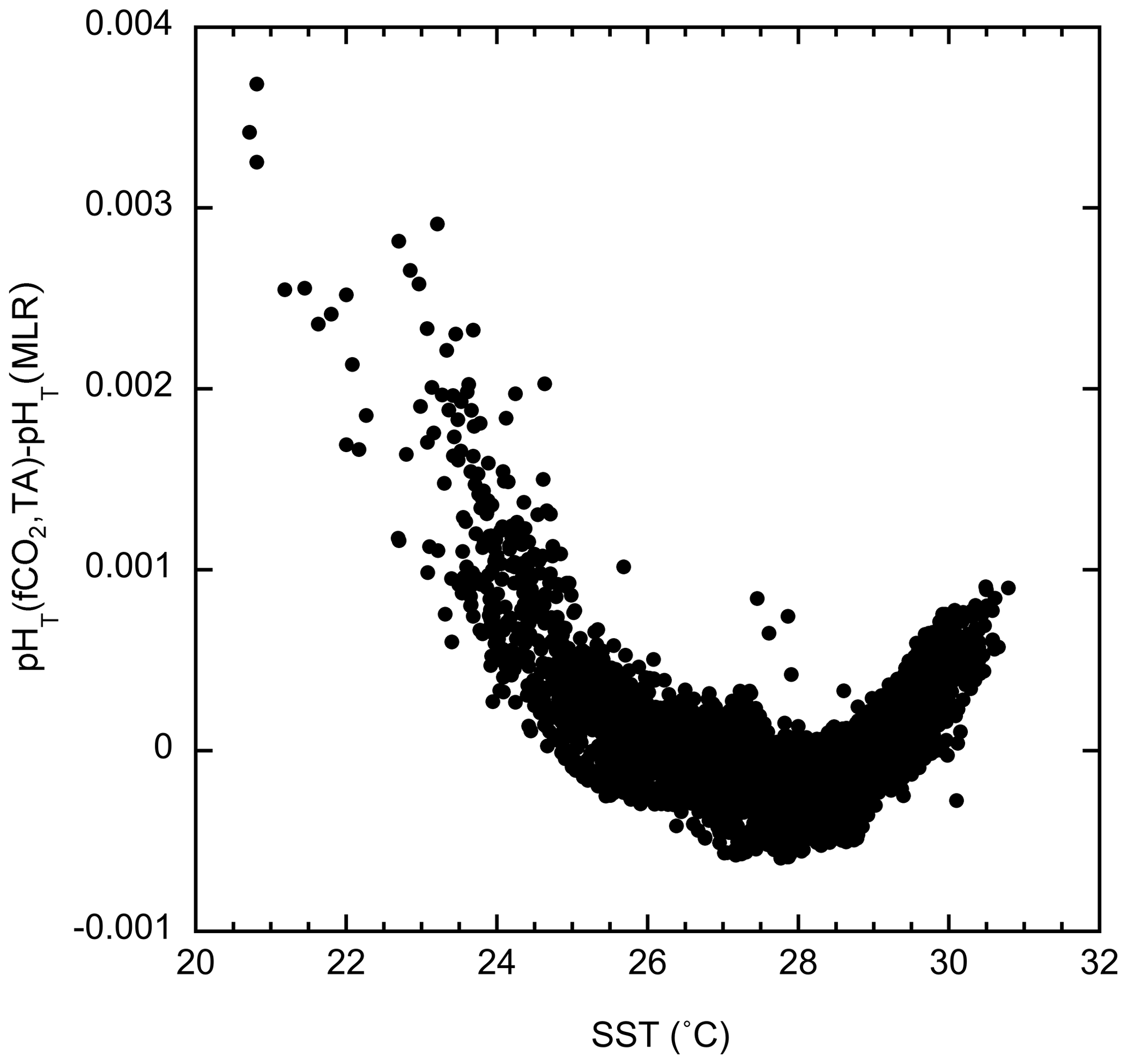
Figure 6 pH_T calculated from gridded fCO_2w and TA estimated from SSS – pH_T(fCO₂,TA) – as done in this work minus pH_T calculated from observed fCO_2w and TA from SSS – pH_T(MLR) – plotted against temperature for the 2017 data.

Table 4 Column headers, units and description for the monthly 1^∘ mapped product (1^∘ by 1^∘ by month) for the whole region.

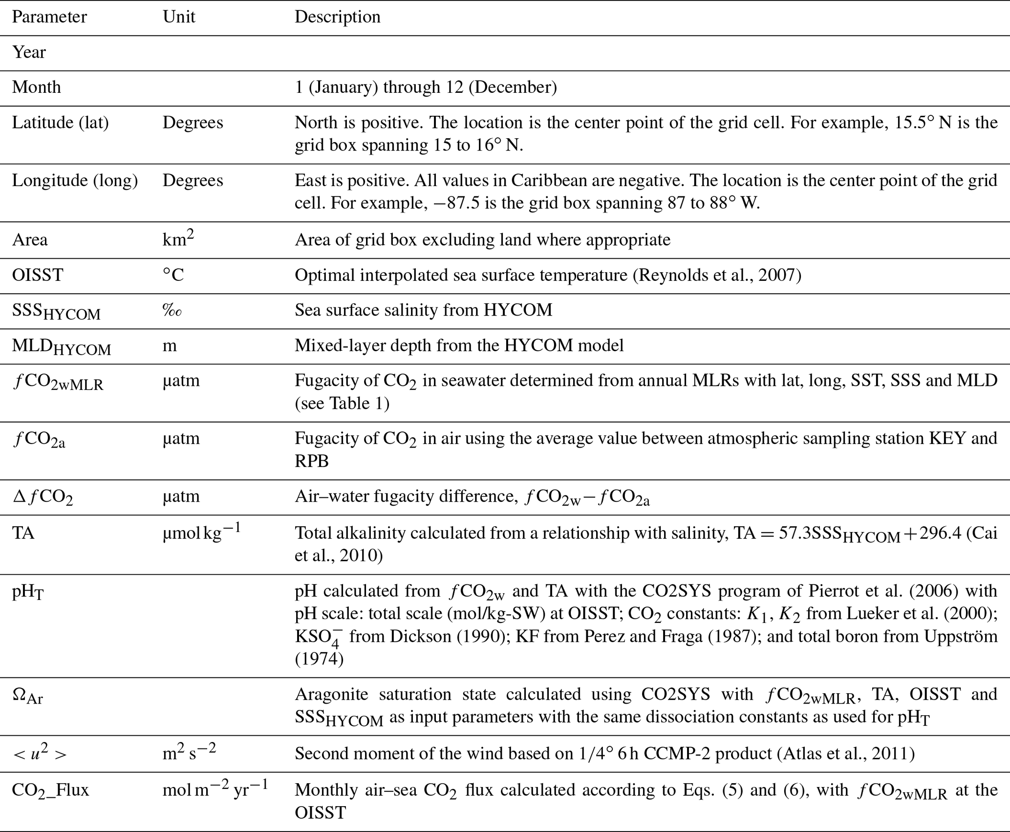
Table 5 Column headers, units and description for the monthly averaged mapped product.

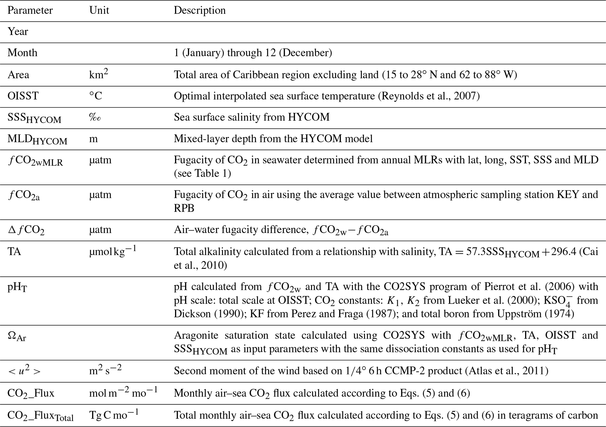
Table 6 Column headers, units and description for the annual averaged mapped product.

Calculated air–sea CO₂ fluxes have a significant uncertainty as they are driven by relatively small air–water concentration differences. Using the uncertainty in fCO_2wMLR of 6.4 µatm, an uncertainty in fCO_2a of 1 µatm, and uncertainties in k of 20 % (Wanninkhof, 2014) and K₀ of 0.002 (Weiss, 1974), the corresponding combined standard uncertainty is 21 % for the flux. For flux calculations the systematic error, or bias, is a big issue. The near-surface temperature gradient and skin temperatures will have an impact on the fCO_2w and K₀. The magnitude, along with its applicability to the bulk flux formulation, is under debate (McGillis and Wanninkhof, 2006; Woolf et al., 2016). For the mapped product, the OISST is used. The OISST uses a variety of temperature data, including remote sensing of the skin temperature, and the product is adjusted to buoy temperatures nominally at 1 m (Reynolds et al., 2007) such that a common reference depth is implicitly used for fCO_2wMLR. As shown in Wanninkhof et al. (2019b) the OISST was on average 0.25 ^∘C lower than SST, and using the SST instead of the OISST would change the flux from −0.87 to −0.63 mol m⁻² yr⁻¹, a 27 % decrease. Using OISST for bulk temperature and a canonical value of 0.17 ^∘C for the difference in bulk and skin temperature would increase the uptake of CO₂ by 18 %, from −0.87 to −1.04 mol m⁻² yr⁻¹. Based on current knowledge, we believe that using the OISST and the resulting calculated fCO_2wMLR as was done here yields the appropriate fluxes.

5 Datasets and data products

Several different data products are provided in conjunction with this paper. The methodology to create the products is described above, and the file format and column headers are presented here with a brief description when warranted.

5.1 Underway fCO₂ data

The quality-controlled cruise data are posted at different locations. The individual cruise files with metadata can be found at https://www.aoml.noaa.gov/ocd/ocdweb/occ.html (last access: 30 June 2020). Data can be found as part of the SOCAT holdings (Bakker et al., 2016) using an interactive graphical user interface (https://ferret.pmel.noaa.gov/socat/las/, last access: 2 July 2020). In addition, cruise files of the three ships are provided in annual directories at the National Centers for Environmental Information (NCEI; https://www.nodc.noaa.gov/ocads/oceans/VOS_Program/explorer.html, last access: 12 April 2020). The data file structures are from the MATLAB data reduction program of Pierrot (Denis Pierrot, personal communication, January 2020). The primary identifier for the cruises is the EXPO code, which is the International Council for the Exploration of the Sea (ICES) ship code and the day the ship starts the cruise. Examples are as follows: for a cruise of the EoS starting on 6 March 2002, the EXPO code is 33KF20020306; for an ALoS cruise starting on 25 November 2018, the EXPO code is BHAF20181125; and for the Eqnx cruise departing her home port on 10 February 2018, it is MLCE20180210. The individual cruise files at the sites above sometimes include data outside the study region.

5.2 Gridded data

The gridded datasets are the binned and averaged fCO_2w, SST and SSS observations on a (1^∘ by 1^∘ by month) grid. The files include the auxiliary data obtained from remote sensing and interpolated data (OISST), data assimilation of remotely sensed winds (CCMP-2), and from the HYCOM model (SSS_HYCOM). TA, pH_T and Ω_Ar calculated using procedures outlined above are provided in the file. The fCO_2w values calculated using the annual MLRs (Table 1) are provided as well. This gridded dataset has spatial and temporal gaps as the ships did not transit through each pixel, and coverage is uneven. The number of observations differs for each grid cell and is listed in the tables of the gridded dataset. For the auxiliary data the number of data points is fixed by the resolution of the data products except where part of the grid includes land, which is masked. The column headers are provided in Table 3 and include units and descriptions when warranted.

5.3 Mapped product

The mapped product provides the data in homogeneous (1^∘ by 1^∘ by month) grid boxes utilizing the annual MLRs of fCO_2w as a function of lat, long, OISST, SSS_HYCOM and MLD_HYCOM for the region from 15 to 28^∘ N and $-\mathrm{62}{}^{\circ }$ to $-\mathrm{88}{}^{\circ }$ (= 62 to 88^∘ W). The modeled and remotely sensed products OISST, SSS_HYCOM and MLD_HYCOM as well as position were used in the MLR (Eq. 4) as the independent parameters. The mapped product includes the air–sea CO₂ fluxes in the region as a specific flux (mol m⁻² yr⁻¹) for each grid box. The column headers are provided in Table 4, including units and descriptions when warranted.

5.4 Monthly and annual estimates for the Caribbean, 2002–2018

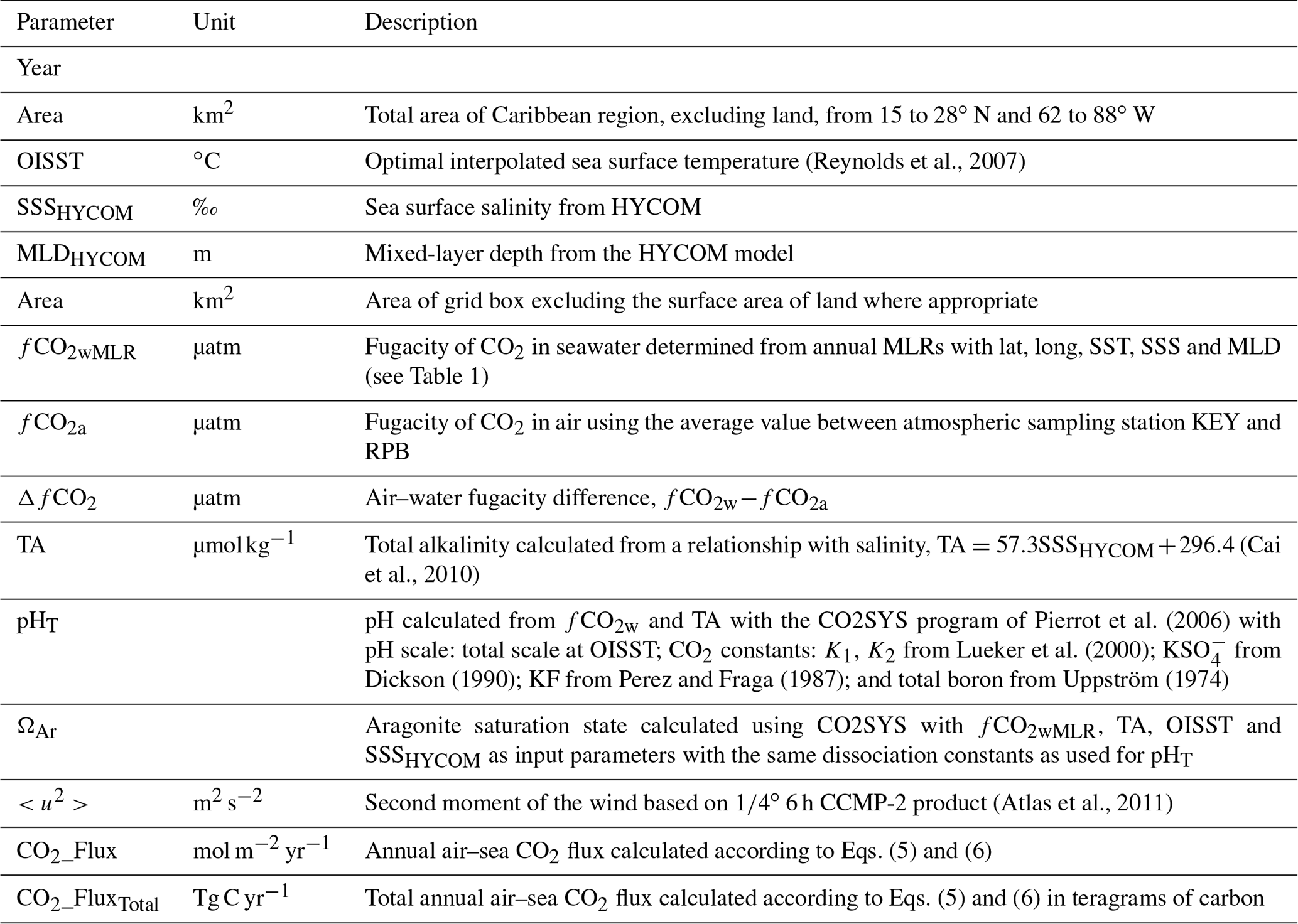
Summary files of monthly and annual data and products covering the whole region from 15 to 28^∘ N and from 88 to 62^∘ W are provided based on the average or the sum of the data in the mapped products. The column headers for the monthly and annual products are similar (Tables 5 and 6). For the monthly files the average of each parameter for each cell is area-weighted based on the area of the cell as provided in the mapped product (Table 4) according to cell area / (total area / number of cells). The total CO₂ mass flux (CO₂_Flux_Total) is the integral of the monthly area-weighted CO₂ fluxes (mol m⁻² yr⁻¹) expressed in teragrams of carbon (=10¹² g C) per month or per year.

6 Data availability

The observations are available at two locations in slightly different formats, but all files are stored by ship and cruise. The data are submitted to SOCAT at least once a year such that they can be posted in the annual updates of SOCAT (https://socat.info, last access: 2 July 2020, Bakker et al., 2016). The permanent depository of the data is at the NCEI, where the data are stored per cruise in directories listed per year (https://www.nodc.noaa.gov/ocads/oceans/VOS_Program/explorer.html, last access: 2 July 2020, Wanninkhof et al., 2020). The gridded observations and mapped products described herein are posted in directories at the AOML and the NCEI. The dataset and derived quantities are provided on a 1^∘ monthly grid at http://accession.nodc.noaa.gov/0207749 (last access: 30 June 2020) (https://doi.org/10.25921/2swk-9w56; Wanninkhof et al., 2019a). The products cover the years 2002 through 2018 and will be updated annually.

7 Conclusions

The datasets from the cruise ships sailing the Caribbean Sea are a rich resource for studying the trends and patterns of inorganic carbon cycling and ocean acidification in the region. The scales of variability and data density are such that the (1^∘ by 1^∘ by month) monthly gridding captures the magnitudes and trends of fCO_2w and derived inorganic carbon products at seasonal to interannual scales. Using annual MLRs to interpolate fCO_2w, with position, SST, SSS and MLD as independent variables, yielded accurate monthly products (Wanninkhof et al., 2019a). A comprehensive investigation of the changes in decadal trends based on the dataset and products was presented in Wanninkhof et al. (2019b). The combined standard uncertainties and systematic offsets of gridding and mapping were estimated from comparing fCO_2w observations with gridded and mapped products including TA, pH_T and Ω_Ar. The MLRs capture the spatial and temporal variability in fCO_2w and calculated pH_T and Ω_Ar well in the region. The datasets and products are invaluable for model initiation and validation and serve as boundary conditions for nearshore fine-scale models.

Appendix A

Multilinear regressions (MLRs) for fCO_2w were applied to the data on a (1^∘ by 1^∘ by month) grid using sequentially fewer independent parameters, and the increase in residual was determined. This analysis was performed as two of the independent parameters used – sea surface salinity (SSS) and mixed-layer depth (MLD) – are modeled, and their accuracy is not readily known. The functional form for the multilinear regression (MLR) fit is

$$\begin{array}{}\text{(A1)}& \begin{array}{rl}f{\mathrm{CO}}_{\mathrm{2}\mathrm{w},\mathrm{MLR}}=& a\mathrm{long}+b\mathrm{lat}+c\mathrm{SST}+\left[d\mathrm{MLD}\right]\\ & +\left[e\mathrm{SSS}\right]+f,\end{array}\end{array}$$

SST is sea surface temperature, long is longitude and lat is latitude. The MLR with the full number of independent parameters is used in the data products described in the main text, and the resulting data products are in Wanninkhof et al. (2019a). The terms in brackets indicate the parameters omitted in the estimates here. The coefficients for the MLRs and their standard errors for each year without MLD as well as the MLRs without MLD and SSS are provided in Tables A1 and A2. SST and location are the strongest predictors of fCO_2w levels in the region. The increase in the average root mean square of the residual or error (RMSE) excluding MLD and SSS in the annual MLRs is shown in Tables A1 and A2. The average RMSE of the calculated fCO_2w,MLR increases by 8±5.5 % by excluding MLD and increases by 11±5.4 % when MLD and SSS are omitted with the annual differences provided in the last column of Tables A1 and A2.

For the entire record, from 2002 to 2018, single regressions of fCO_2w with position, SST, SSS and MLD showed larger standard errors and coefficients of determination (r²) as they do not capture the increase in fCO_2w over time due to fCO_2w increases in response to increasing atmospheric CO₂ levels. Regressing against ΔfCO₂, which in principle should not have a trend over time if surface water CO₂ levels keep up with atmospheric CO₂ increases, did not improve the correlation with the independent parameters. This was attributed to the relatively small magnitude of ΔfCO₂ and the observed multiyear changes in trends of fCO_2w (Wanninkhof et al., 2019b). However, using the year as a variable in the regression provides a reasonable means of extrapolating over the entire time–space domain with a single regression from March 2002 through February 2018:

$$\begin{array}{}\text{(A2)}& \begin{array}{rl}f{\mathrm{CO}}_{\mathrm{2}\mathrm{w},\mathrm{MLR}}& (\pm \mathrm{7.8})=\mathrm{23.3}(\pm \mathrm{2.0})+\mathrm{1.45}(\pm \mathrm{0.02})\\ & (\mathrm{YR}-\mathrm{2002})+\mathrm{10.23}(\pm \mathrm{0.06})\mathrm{SST}\\ & +\mathrm{1.19}(\pm \mathrm{0.03})\mathrm{lat}\\ & -\mathrm{0.50}(\pm \mathrm{0.01})\mathrm{long},r^{\mathrm{2}}=\mathrm{0.84},\end{array}\end{array}$$

where YR is the integer calendar year. Thus (YR-2002) is the year since the start of the record. The coefficient for the (YR-2002) term of 1.45 reflects the annual increase in surface water fCO_2w due to atmospheric fCO_2a increase, which averages 2.1 µatm yr⁻¹ over the 2002–2018 time period.

The standard error in the fCO_2w,MLR of 7.8 µatm in Eq. (A2) is generally greater than the standard error in the annual algorithms used to fill the gaps for the annual estimates (Eq. A1) that range from 4.7 to 9.9 µatm, depending on the year, with an average of 6.4 µatm (Table 1 in main text).

The importance of the different independent variables for the fCO_2w,MLR can, in part, be discerned from the standard error in the coefficients, but since variables are cross-correlated, other means are investigated, such as creating an MLR with either a subset or substitution of variables. Physical parameters were correlated with location (lat, long) in the region. In particular, salinity showed broad correspondence with position. Therefore, substituting SSS for lat and long provided a similar magnitude and standard error in the coefficients of the independent variable but a 10 % greater root mean square (rms) in the estimated fCO_2w :

$$\begin{array}{}\text{(A3)}& \begin{array}{rl}f{\mathrm{CO}}_{\mathrm{2}\mathrm{w},\mathrm{MLR}}& (\pm \mathrm{8.8})=-\mathrm{238}(\pm \mathrm{9.8})+\mathrm{1.36}(\pm \mathrm{0.02})\\ & (\mathrm{YR}-\mathrm{2002})+\mathrm{10.11}(\pm \mathrm{0.06})\mathrm{SST}\\ & +\mathrm{9.07}(\pm \mathrm{0.25})\mathrm{SSS},r^{\mathrm{2}}=\mathrm{0.79}.\end{array}\end{array}$$

Finally, a simple two-parameter linear fit with YR and SST had reasonable predictive capability:

$$\begin{array}{}\text{(A4)}& \begin{array}{rl}f{\mathrm{CO}}_{\mathrm{2}\mathrm{w},\mathrm{MLR}}& (\pm \mathrm{9.4})=\mathrm{107.2}(\pm \mathrm{1.7})+\mathrm{1.38}(\pm \mathrm{0.02})\\ & (\mathrm{YR}-\mathrm{2002})+\mathrm{9.50}(\pm \mathrm{0.06})\mathrm{SST},r^{\mathrm{2}}\\ & =\mathrm{0.77}.\end{array}\end{array}$$

Equation (A4) uses only SST, and time showed an increase in the standard error of the derived independent variable fCO_2w compared to the other permutations of the MLR. This simple relationship did show some biases with location (not shown), and for gap filling to create uniform monthly fields of fCO_2w, the full annual regressions (Table 1) using all independent parameters – SST, SSS, MLD and location – were the best option.

Table A1 Coefficients for the MLR, fCO_2w,MLR = a long + b lat + c SST + e SSS + f.

^a The second row (in italics) for each annual entry is the error of the coefficient. ^b The increase in root mean square error (RMSE) of fCO_2w,MLR compared to Table 1, which includes MLD as an input.

Table A2 Coefficients for the MLR, fCO_2w,MLR = a long + b lat + c SST + f.

^a This table is the same as Table A1 except that MLD in addition to SSS is omitted as an independent variable. ^b The increase in root mean square error (RMSE) of fCO_2w,MLR compared to Table 1, which included MLD and SSS as independent variables. ^c The second row (in italics) for each annual entry is the error of the coefficient.