the Creative Commons Attribution 4.0 License.
the Creative Commons Attribution 4.0 License.
 | 30 Jun 2020
Rescue and quality control of sub-daily meteorological data collected at Montevergine Observatory (Southern Apennines), 1884–1963
Vincenzo Capozzi
Yuri Cotroneo
Pasquale Castagno
Carmela De Vivo
Giorgio Budillon
Here we present the rescue of sub-daily meteorological observations collected from 1884 to 1963 at Montevergine Observatory, located in the Southern Apennines in Italy. The recovered dataset consists of 3-daily observations of the following atmospheric variables: dry-bulb temperature, wet-bulb temperature, water vapour pressure, relative humidity, atmospheric pressure, cloud type, cloud cover, rainfall, snowfall and precipitation type. The data, originally available only as paper-based records, have been digitized following the World Meteorological Organization standard practices. After a cross-check, the digitized data went through three different automatic quality control tests: the gross error test, which verifies whether the data are within acceptable range limits; the tolerance test, which flags whether values are above or below monthly climatological limits that are defined in accordance with a probability distribution model specific to each variable; and the temporal coherency test, which checks the rate of change and flags unrealistic jumps in consecutive values.
The result of this process is the publication of a new historical dataset that includes, for the first time, digitized and quality-controlled sub-daily meteorological observations collected since the late 19th century in the Mediterranean region north of the 37th parallel. These data are critical to enhancing and complementing previously rescued sub-daily historical datasets – which are currently limited to atmospheric pressure observations only – in the central and northern Mediterranean regions. Furthermore, the Montevergine Observatory (MVOBS) dataset can enrich the understanding of high-altitude weather and climate variability, and it contributes to the improvement of the accuracy of reanalysis products prior the 1950s. Data are available on the NOAA's National Centers for Environmental Information (NCEI) public repository and are associated with a DOI: https://doi.org/10.25921/cx3g-rj98 (Capozzi et al., 2019).
- Article
(2764 KB) - Full-text XML
- BibTeX
- EndNote


Historical meteorological records stretching back to the 19th century are crucial for the comprehension of climate variability and its long-term change. These data provide an essential baseline of past climate, which can be useful for many initiatives and efforts focused on monitoring and adapting to climate change and extreme weather events. Thus, the process of past meteorological data retrieval and digitizing, known as “data rescue”, is receiving more and more interest within the scientific community, as proven by the high number of projects funded in the last 2 decades. Examples are the Atmospheric Circulation Reconstructions over the Earth (ACRE; Allan et al., 2011), the Mediterranean Data Rescue (MEDARE) and the Historical Instrumental Climatological Surface Time Series of the Greater Alpine Region (HISTALP) initiatives (Auer et al., 2007; Brunet et al., 2014a, b). These projects as well as other actions led by local meteorological agencies and research institutions have two main tasks: (i) to enhance past weather observation assets (in part still unexplored) by discovering, preserving and digitizing paper-based data and (ii) to ensure through quality control procedures that the recovered data are consistent and fully available to the scientific community.
Most of data rescue initiatives are focused on daily and monthly atmospheric observations used for long-term climatological analysis (i.e. daily maximum, minimum and average temperature as well as daily and monthly total precipitation), but few actions have been established to recover sub-daily data. High-temporal-resolution weather data are pivotal to understanding the dynamics related to atmospheric circulation and to extreme weather events (e.g. Stickler et al., 2014; Wetra et al., 2014). Thus, sub-daily data constitute a key input for reanalysis products at both the global and regional scale. A significant effort to rescue historical sub-daily data has been made by the Twentieth Century Reanalysis (20CR) and the Uncertainties in Ensembles of Regional Reanalyses (UERRA) projects. The 20CR product is the first ensemble of sub-daily global atmospheric conditions (Compo et al., 2011; Cram et al., 2015; Slivinski et al., 2019) spanning from 1851 to 2014 (20CR version 3). This project supported national and regional initiatives focused on the recovery of sub-daily data extending back to the 19th century. The 20CR project is aimed exclusively at the assimilation of atmospheric pressure observations (Slivinski et al., 2019); thus the resulting observational database is limited to this variable.
On the other hand, the aim of the UERRA project is to develop an ensemble system of regional European reanalyses for recent decades (1961–2019) through the recovery of sub-daily, multi-parametric surface weather records (http://uerra.eu/, last access: 31 January 2020). Within the framework of the UERRA project, Ashcroft et al. (2018) identified for the 1957–2010 period a relevant scarcity of sub-daily data in different areas in and around Europe, including southern and eastern Mediterranean countries (Morocco, Algeria, Tunisia, Egypt and Turkey), Central and Eastern Europe (Germany, Czech Republic, Hungary and the Balkan Peninsula), and Scandinavia. To fill these gaps, the rescue of 8.8 million observations covering a period from 1877 to 2012 and encompassing a wide range of meteorological variables was carried out.
Despite this relevant effort, the availability of sub-daily meteorological data collected from the late 19th century remains inadequate over most of the European territory. A lack of data is particularly evident in the Mediterranean region, where few long-term records are available in digital format despite the rich and invaluable heritage of historical meteorological surface data (Brunet et al., 2014b; Libertino et al., 2018). Figure 1a provides clear evidence of the current situation in the Mediterranean area in terms of digitized and publicly accessible sub-daily time series for the period ranging from the late 1800s to the 1960s. This figure shows the 26 historical stations extracted from the International Surface Pressure Databank version 4.7 (ISPDv4) and from Ashcroft et al. (2018) datasets, from which sub-daily meteorological data are already available in digital format for the period 1884–1963. The ISPDv4 is an international repository in which several national and international historical data collections are converged (Compo et al., 2019). This database incorporates all the observations assimilated by 20CR version 3 (Slivinski et al., 2019) and constitutes the world's largest database of atmospheric pressure data. The majority of the stations (58 %) include only atmospheric pressure data (blue dots) and are mainly located in southern Italy, north-western Italy and the Balkan region. The remaining 42 % of the stations (red dots) include multi-parametric meteorological observations recovered by Ashcroft et al. (2018) and are mainly located in southern Mediterranean regions (Algeria, Tunisia and Cyprus).
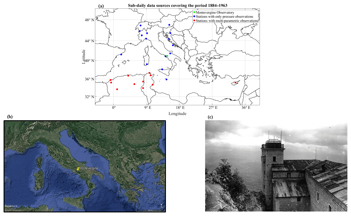
Figure 1Panel (a): map of Mediterranean region showing the location of sub-daily meteorological data available in digital format for the period 1884–1963. Blue dots represent the stations including only atmospheric pressure measurements, and red dots represent the stations for which multi-parametric meteorological observations are available. Data sources have been provided by the International Surface Pressure Databank version 4.7 (Compo et al., 2019; https://rda.ucar.edu/datasets/ds132.2/index.html?sstn=17606&spart=exact stationVie, last access: 29 January 2020) and by Ashcroft et al. (2018) datasets. Panel (b) shows the central Mediterranean region, including Montevergine (highlighted via a yellow pin). Montevergine is also marked in panel (a) as a green dot. Image credits: © Google Earth, Data Sio, NOAA, U.S. Navy, NGA, GEBCO. Panel (c) presents an old photo of the Montevergine Observatory tower, situated near the top of the Partenio mountain chain on the north-eastern side of the Montevergine abbey. Image courtesy of the Italian Air Force (http://www.meteoam.it/page/montevergine, last access: 25 April 2020).
Our work aims to partially fill the relevant lack in sub-daily data availability prior to the 1960s, presenting the rescue of sub-daily meteorological observations collected at Montevergine Observatory (MVOBS) from 1884 to 1963. MVOBS is located in the Campania region (40.936502∘ N, 14.729150∘ E) at 1280 m above sea level (a.s.l.), near the top of the Partenio mountains, which are part of Southern Apennines in Italy (Fig. 1b). The rescued sub-daily dataset includes 3-daily observations of several atmospheric parameters, namely dry-bulb temperature, wet-bulb temperature, water vapour pressure, relative humidity, atmospheric pressure, cloud type, cloud cover, rainfall, snowfall and precipitation type.
In accordance with the ISPDv4 database, there are only five other historical weather stations in southern Italy extending back several decades prior to the 1960s that had performed sub-daily multi-parametric observations and that may supply digitized data: Naples Capodimonte (40.88∘ N, 14.25∘ E), Foggia Nigri (41.46∘ N, 15.54∘ E), Taranto Ferrajolo, (40.47∘ N, 17.23∘ E), Palermo (38.10∘ N, 13.35∘ E) and Cagliari (39.20∘ N, 9.15∘ E). They are all located in coastal or near-coastal areas and only provide atmospheric pressure data with a temporal resolution of one observation per day (https://rda.ucar.edu/datasets/ds132.2/index.html?sstn=17606&spart=exact stationVie, last access: 29 January 2020). The digitized records available for these stations cover the period 1895–1940, except for the Taranto observatory, whose time series spans a very limited time interval (1931–1939). For this reason, it has not been included in Fig. 1a.
In light of the above, the sub-daily data rescue activities carried out in southern Italy until now are incomplete. Furthermore, these datasets available in a digital format are only a small part of the larger amount of meteorological information stored in the original paper archives in terms of both data temporal resolution and number of measured atmospheric parameters.
The sub-daily multi-parametric rescued dataset in this study (green dot in Fig. 1) is the first dataset for the Mediterranean region north of the 37th parallel dating back to the late 19th century to have been digitized, quality-controlled and made publicly accessible.
Therefore, MVOBS data enhance and supplement historical sub-daily datasets currently available in southern Italy and in the Mediterranean region, broadening the meteorological parameter spectrum and extending the current knowledge of past climate variability to the inland and mountainous sectors.
The sub-daily meteorological records collected at MVOBS have been recovered by the Department of Science and Technology of the University of Naples “Parthenope” within the framework of the EPIMETEO project, which aims to characterize the past and present weather conditions in the Campania region.
As already observed by many authors (Diodato, 1992; Capozzi and Budillon, 2013, 2017), using daily meteorological parameter data only, MVOBS makes a crucial contribution to the study of climate variability.
Distinguishing MVOBS features have been synthesized in the following key points:
- (a)
The MVOBS sub-daily multi-variable dataset offers a rare opportunity to investigate climate features of the central Mediterranean mountain environment prior to the 1950s. Mountainous areas are particularly vulnerable to climate change, which has severe impacts on high-altitude ecosystems and habitats (Abeli et al., 2012). In many areas, a solid assessment of mountain climate variability propaedeutic to the development of reliable future scenarios is difficult due to the scarcity of available data and information.
- (b)
MVOBS is the only meteorological observatory among those operating in Apennine regions at elevations above 1000 m a.s.l. to provide a climatological time series extending back to the late 19th century. According to Brunetti et al. (2006), high-altitude (>1000 m a.s.l.) time series comparable in length with the MVOBS record can be found in Italy only in the Alpine region.
- (c)
The MVOBSV dataset, collected near the top of the atmospheric-boundary layer, allows a proper and objective characterization of air masses as well as of atmospheric transients that have driven central Mediterranean meteorological scenarios from 19th century to early 1960s.
- (d)
Finally, the MVOBS time series has been measured in a location whose features have remained unchanged over time due to the absence of urban settlements. Therefore, these rescued climatic records can be considered devoid of local non-climatic effects related to urbanization, which may cause inhomogeneity in the time series (e.g. Jones et al., 1990).
MVOBS can be considered an ideal site for the study of climate variability in a “local-to-global framework”. In other words, MVOBS records, collected in a remote high-altitude location, allows the investigation of the relationship between local- and global-scale climate change. Moreover, MVOBS data can shed light on the mutual interactions between large-scale synoptic flow and local orographic features and how these interactions have changed over time due to the variations and anomalies of atmospheric circulation.
Following the standards suggested by the World Meteorological Organization (WMO) and the common practices used in climatological data recovery projects, we have structured the rescue of MVOBS dataset into three different steps:
- i.
identification of metadata (i.e. the information about the history of the station, the instrumentation, the observation practices, the measured atmospheric parameters and the site condition) and data sources;
- ii.
digitization of original paper-based data;
- iii.
quality control and assurance assessment of digitized data through visual inspection and objective statistical methods.
This paper is organized as follows. Section 2 deals with the first two steps of data rescue, providing information about MVOBS history, metadata, availability of meteorological variables and digitizing methodology. Section 3 describes the quality control procedures, and Sect. 4 presents some examples of the use of this dataset. Concluding remarks are made in Sect. 5.
2.1 MVOBS history and measurement practices
The first step of the data rescue process consisted of the identification of metadata that can have an impact on data collection (location of instruments, changes in practice etc.). We conducted a careful examination of the bibliographic documents stored in the MVOBS archive located at the Montevergine abbey. The metadata of the MVOBS sub-daily dataset have been retrieved from two old hand-written diaries, named Le Cronache dell'Osservatorio. Such manuscripts started in 1938 and contain a year-by-year “observatory chronicle” for the period 1881–1946. In order to trace the history of MVOBS before 1938, the authors used different sources: postal correspondence, verbally transmitted news, and a pamphlet entitled Nel Cinquantenario dell'Osservatorio Meteorologico di Montevergine 1884–1934 (The 50th anniversary of Montevergine meteorological observatory 1884–1934), published in 1934 on the observatory's 50th anniversary. For the period after 1946, metadata have been retrieved from the meteorological observation registers and from another pamphlet named Osservatorio meteorologico Santuario di Montevergine (Montevergine abbey meteorological observatory) that was published in 1984 to celebrate the centenary of MVOBS. During the metadata recovery process particular attention was given to the assessment of factors that may cause inhomogeneity in the time series, such as instrument relocation and replacement as well as change in the personnel responsible for the meteorological observations.
According to the old diaries, the idea of establishing a meteorological specola in Montevergine was conceived in 1881 by Father Francesco Denza, a meteorologist belonging to the religious order of Barnabiti (i.e. Catholic priests and religious brothers belonging to the Roman Catholic religious order of the Clerics Regular of St. Paul). The MVOBS weather observations started 3 years later on 1 January 1884. MVOBS was part of the first Italian meteorological institution, the “Italian Central Office of Meteorology and Geodynamics” (hereafter the Italian Central Office, ICO), established in Rome in 1879 (Maugeri et al., 1998). In the period 1884–1894, a room located at the north-facing front of the Montevergine monastery was dedicated to the monitoring of weather conditions. Unfortunately, during this period no specific information about the instruments' positioning was recorded. From 1895, the data were collected in a meteorological tower built on the eastern side of the abbey at the suggestion of the ICO. The square-based tower measures 28.4 m in height and 5.7 m in width and was equipped with a Stevenson screen located outside a north-facing window (Fig. 1b). The shelter hosted the following instruments: a maximum and minimum thermometer, a thermograph, a psychrometer and an evaporimeter. Other instruments, e.g. the rain gauge, the anemograph and the nephoscope, were placed on the observatory terrace at the top of the tower. The barometer, the barograph and the recording pluviograph were installed in the observatory room, located on the highest floor of the tower. The nivometric measurements, in compliance with the recommendations of the ICO, were performed using a traditional nivometer consisting of a yardstick and a snowboard with a section of 0.0001 m2 and an area of 0.01 m2, respectively. However, no detailed, precise information about the nivometer positioning was found. According to verbally transmitted information (supplied to the authors of this work by the Benedectine community of Montevergine), the snow observations may have been collected in the Giardinetto dell'Ave Maria, a cloister of the Montevergine abbey located near the northern side of the meteorological tower. Additional historical photos showing the observatory room, the meteorological tower and the surrounding environment as well as a modern panoramic view of the Montevergine abbey are offered in Appendix A.
The weather observations were performed by the Benedictine community of Montevergine under the guidance of a monk (the observatory director) trained by the ICO.
Table 1 provides a summary of the metadata information retrieved for the investigated period (1884–1963). Unfortunately, no relevant and useful information was found for the period 1896–1926 except for a change in observatory guidance in 1919. The diaries documented the restoration of the observatory rooms in 1926 and the replacements of some instruments in 1927, 1931, 1937, 1941, 1945 and 1958. From November 1930 to April 1931, the observatory activities were temporarily interrupted. In 1938, MVOBS also became part of the Regia Aeronautica meteorological network (the modern “Meteorological Service of the Italian Air Force”). The observatory served the military institution until March 1952, producing and transmitting six additional bulletins per day (unfortunately not preserved in the observatory archive).
Table 1Summary of documented metadata in the period from 1884 to 1963. The information about change in instrument relocation and replacement, change in observatory guidance, and site measurement conditions was retrieved from the old Le Cronache dell'Osservatorio diaries and from the meteorological observation registers.
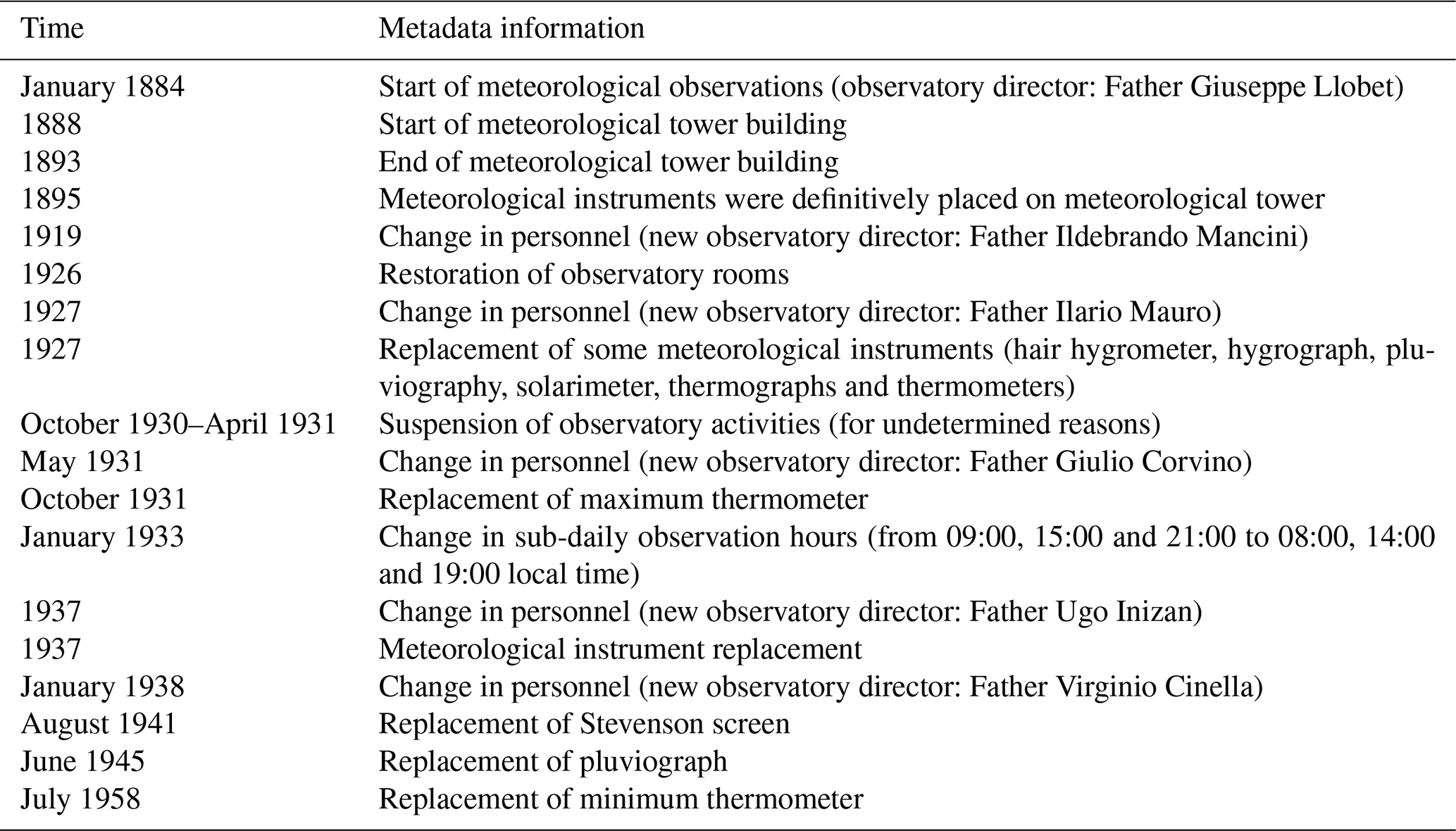
According to the norms prescribed by the ICO, from 1884 to 1932 sub-daily meteorological observations were measured at 09:00, 15:00 and 21:00 local time. From 1933 new standards were adopted by the ICO and the sub-daily data were recorded until 1963 at 08:00, 14:00 and 19:00 local time. These observations include 16 different meteorological parameters (see Fig. 2 for data availability periods). Near-continuous observations (i.e. measurements characterized by an availability greater than 90 %) are available for the following variables: dry-bulb temperature, wet-bulb temperature, water vapour pressure, relative humidity, atmospheric pressure, cloud type, cloud cover, accumulated rainfall and snowfall, and precipitation type. Additional but incomplete or sporadic sub-daily observations involved the wind direction and speed, cloud direction, snow depth (only recorded in the periods November 1944–March 1952 and November 1953–May 1961), visibility, and low-level cloud base height and quantity (only observed in the period August 1955–May 1961).

Figure 2Data availability of the MVOBS sub-daily dataset in the period ranging from 1884 to 1963. Near-continuous observations are available only for the following variables: precipitation type, cloud cover and type, dry-bulb temperature, atmospheric pressure, vapour pressure, relative humidity, rainfall, and snowfall.
In the 1884–1963 period, near-continuous daily observations of the following parameters were also carried out: maximum temperature, minimum temperature, accumulated rainfall and snowfall, and precipitation event duration. Minimum and maximum temperatures were observed at 15:00 and 21:00 local time (14:00 and 19:00 local time from 1933), respectively. For short periods, the daily observations also included evaporation (from 1884 to 1920), maximum hourly precipitation (from 1941 to May 1961) and snow depth (from 1937 to 1963).
On May 1964, due to a lack of personnel, the meteorological observations for the ICO were suspended. The activities were suspended until 1968 and then restored in the subsequent year upon the proposal of the Servizio Idrografico del Genio Civile di Napoli. However, from 1969 to 2007, only daily observations of the main meteorological variables (maximum and minimum temperature, accumulated rainfall and snowfall, and precipitation type) were performed. Although the observatory is no longer part of any institutional meteorological network, it has continued its activity through an automatic weather station (AWS) with the scientific support of the Department of Science and Technology of the University of Naples “Parthenope” since 2008. The AWS was installed on the observatory terrace and archives several meteorological parameters (temperature, precipitation, pressure, solar radiation, wind direction and wind speed) with a temporal resolution of 1 min. MVOBS is also presently equipped with a laser optical disdrometer, mainly used to retrieve measurements of liquid-equivalent water snowfall rate (Capozzi et al., 2020).
2.2 Data sources and digitization
The data rescued in this study are stored in 80 paper-based registers, each containing the daily and sub-daily observations collected for each year of the investigated period. A single register consists of 24 pages (two pages for every month) and is formatted in tables according to the standards suggested by the ICO. Figure 3 presents an extract of the meteorological register for the data measured in March 1892. Each table is related to a month, comprising two pages: the first column of each table lists the days, and the first row lists the name of the parameters and observation time. Each box in each column contains the value of a certain parameter at a specific time of the day. As an example, on the first page (Fig. 3a) the first column (from left) lists the days of the month, and columns 2 to 10 provide atmospheric pressure observations. The barometer temperature, measured atmospheric pressure and corrected atmospheric pressure are reported for each observation time (09:00, 15:00 and 21:00 local time). The 11th column is the average of the 3-daily corrected pressure observations. Columns 12 to 17 contain the psychrometric measurements (dry- and wet-bulb temperature) for each of the 3-daily observations. The 18th column shows the average of the sub-daily psychrometric records, and columns 19 and 20 are dedicated to daily minimum and maximum temperature, respectively. The sub-daily observations of vapour pressure and relative humidity as well as their daily average are reported in columns 21–24 and 25–28, respectively. On the following page (Fig. 3b), the first column lists the days of the month. Columns 2 to 7 show sub-daily observations of wind direction and speed. From columns 8 to 10, upper wind (or cloud direction) measurements are listed. Columns 11 to 19 report sky and weather conditions: each triplet includes cloud cover, cloud type and hydrometeor observations for a specific time. The hydrometeors column also contains information about the accumulated snowfall and rainfall between two consecutive sub-daily observations. The average of 3-daily cloud cover records is listed in column 20. It is important to highlight that sky conditions, i.e. cloud cover and type, were assessed by visual observations. According to this empirical approach, cloud amount was estimated by evaluating the portion of sky covered by clouds. The reference scale for recording the cloud coverage (WMO, 2014) is expressed in tenths and ranges from 0/10 (sky completely clear) to 10/10 (overcast). To detect the cloud type, various classification methods, which considered cloud species (shape and structure), variety (cloud arrangement and transparency) and cloud level (high, medium and low), were used. Daily accumulated rainfall data and precipitation duration are listed in columns 21–22, and daily accumulated snowfall and evaporation are shown in columns 23–24. Finally, columns 25–26 report ozone observations (never available in MVOBS dataset).
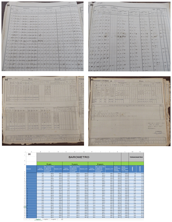
Figure 3The upper (a, b) and middle (c, d) panels show an example of the original data source (March 1892 and January 1946, respectively). Each row accounts for the observations of a specific day including their average on a decadal and monthly basis, and each column is devoted to the records of a determined parameter at a specific hour of the day. The bottom panel (e) is an example (referring to data collected in March 1892) of the template used in the data digitization. The rows are designed to match the location of the data in the original source.
The described data format is representative of the analysed period except from November 1952 to October 1953 and from March 1962 to December 1963, when a different format was used, and the meteorological parameters were sampled only once a day. Moreover, the meteorological registers of the 1944–1961 period contain additional columns dedicated to other (sporadically measured) variables such as snow depth, visibility, and low-level cloud base height and quantity. Those registers have a different structure from the standard format described previously. Indeed, a single register consists of 72 pages (i.e. two pages for every 10-day period of each month), and each page contains two tables. Panels (c) and (d) in Fig. 3 show the register structure for the second 10-day period (i.e. from day 11 to 20) of January 1946. In particular, the upper table on the left page (Fig. 3c) includes 3-daily observations of atmospheric pressure, wind direction and force, and cloud direction performed from day 11 to 20. The bottom table shows daily maximum and minimum temperature, 3-daily observations of dry- and wet-bulb temperature, vapour pressure, relative humidity, and finally the sum and average of thermometric measurements. The upper table on the right page (Fig. 3d) contains sub-daily records of the sky conditions (cloud cover and type), accumulated rainfall, snow depth and accumulated snowfall. In addition, daily summaries related to cloud cover, accumulated rainfall and snowfall, maximum 1 h rainfall amount, and precipitation duration (hours and minutes) are reported. The bottom table is dedicated to special notes concerning observed hydrometeors and meteorological phenomena.
The digitization of the MVOBS dataset available from the NOAA's National Centers for Environmental Information (NCEI) repository (Capozzi et al., 2019) was handled by the personnel involved in this study. A simple “key entry” approach has been used to transcribe the data into a digital format. Among the techniques generally employed for climate data digitization, this method is slower in terms of the amount of digitized data per hour (Brönnimann et al., 2006); however, at the same time, such a method has the lower error rate and follows the standard practices recommended by the WMO (2016). The digital templates, developed in Microsoft Excel (Fig. 3e), have been structured in a format that is very similar to the original data source in order to help the digitizers in keeping track of their work. Digitized data have been cross-checked with the original source values at the end of every rescued month to identify and remove transcription errors.
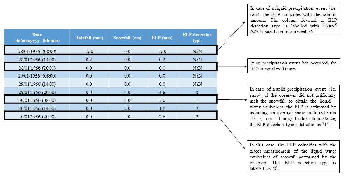
Figure 4Summary of the strategy used to assess the equivalent liquid precipitation (ELP) parameter. The left table has been obtained by adapting an extract of the digital version of the MVOBS dataset available from the NOAA's NCEI repository (Capozzi et al., 2019). It lists the sub-daily precipitation data observed between 28 and 30 January 1956. From left to right: rainfall (mm), snowfall (cm), ELP (mm) and ELP detection type (expressed as a numeric or textual label). The rows highlighted in black present different ELP estimation scenarios.
In order to speed-up the digitization process and to improve the accuracy of the rescued data, we have automatized the transcription of some indirectly measured variables, i.e. the corrected atmospheric pressure, the vapour pressure and the relative humidity. The first variable has been determined according to the following relationship (Brombacher et al., 1960):
where P0 is the corrected atmospheric pressure (mmHg), i.e. the atmospheric pressure reduced to standard temperature (∘C); P is the observed pressure (mmHg); and CT is a temperature correction factor. The latter is defined as
where a is the coefficient of expansion for mercury (0.0001818); b the coefficient of linear expansion of brass (0.000184); and Tb is the barometer temperature, measured by an attached thermometer.
Well-known psychrometric formulae have been used to automatically retrieve vapour pressure and relative humidity data. More specifically, the partial pressure of water vapour (e) has been obtained as follows (WMO, 2014):
where T is the air temperature (dry-bulb temperature), Tw is the wet-bulb temperature, and ew (Tw) is saturation vapour pressure with regard to water at the wet-bulb temperature. ew (Tw) has been determined according to the following relationship:
Finally, relative humidity (RH) has been obtained as , where ew(T) is the saturation vapour pressure with regard to water at the dry-bulb temperature.
Moreover, during the digitization process, special attention was dedicated to the information concerning the equivalent liquid water of the accumulated snowfall. This information is essential to reliably characterize the pluviometric regime variability and trend of high-altitude environments (where a large part of winter precipitation falls as snow). The weather observers operating at MVOBS did not take an unambiguous and homogeneous approach to assess the snow-to-liquid equivalent amount. In addition, in many cases they omitted such valuable information. To overcome this issue, we created a dedicated column for the equivalent liquid precipitation (ELP) in the digital template. The ELP corresponds to the accumulated rainfall only when liquid precipitation events occur, whereas in the case of solid precipitation events it represents the amount of liquid precipitation after melting snow. When the observers did not record and note the equivalent in liquid of snowfall, we manually estimated the ELP using an average snow-to-liquid-water ratio of 10:1, which means that the melting of 1 cm of snowfall would produce 1 mm of liquid water (e.g. Winiger et al., 2005; Egli, 2008; Egli et al., 2009). It is worth bearing in mind that converting snow to equivalent liquid water is strictly dependent on the snowflakes' wetness: in wet snow circumstances, the ratio decreases and is on average 5:1, whereas in dry snow conditions the ratio is higher (it can be 30:1 or greater) because the snow includes a lower liquid water content. Whenever directly measured by observers, the ELP associated with a determined snowfall event was noted in the original hand-written meteorological registers in the column devoted to accumulated rainfall. To better discriminate between rainfall and liquid equivalent of solid precipitation, we decided to store such data only in the ELP column of our digital template. The strategy used to assess the ELP parameter is synthesized in Fig. 4, which shows an adapted extract of the rescued MVOBS dataset (available from the NOAA's NCEI repository; Capozzi et al., 2019) focusing on the precipitation measurements collected between 28 and 30 January 1956.
The third part of our work deals with the development of a rigorous quality control (QC) procedure, aimed to ensure the consistency and the traceability of the rescued sub-daily dataset (WMO, 2008).
Errors and artefacts in historical climatological time series arise mainly from instrument failures, human mistakes during data collection, inaccuracies in manual data transcription on original sources and digitization. As highlighted by Ashcroft et al. (2018), a comprehensive and reliable QC procedure should be able to identify both systematic and non-systematic errors that may undermine the analysis of climatic signals in a time series.
Steinacker et al. (2011) provided a comprehensive review of the QC strategies usually employed in the meteorological field. Depending on the nature of the data, different approaches can be used. As an example, a large dataset characterized by high data density in space and time allows the selection of sophisticated QC methods, which are able not only to flag an erroneous value but also to correct it through spatial consistency checks. The MVOBS dataset, consisting of observations from a single isolated time series, fits better with simpler QC techniques that can only accept or reject an observation according to objective statistical criteria.
We decided to structure the QC strategy into four different steps consisting of a basic visual check and three different statistical and automatic tests:
- i.
The gross error test flag data that are above or below acceptable physical limits (this step also involves an inter-variable check focused on meteorological parameters that are related by physical constraints).
- ii.
The tolerance test detects the outliers, i.e. data that exceed monthly climatological limits defined according to an objective probability distribution model (specific to each of the investigated meteorological parameters).
- iii.
The temporal coherency test identifies unrealistic “jumps” between two consecutive observations according to the climatological change that might be expected for a determined variable in a specific time interval.
A schematic diagram of the quality control procedure applied to MVOBS sub-daily data is presented in Fig. 5. According to the results achieved from the different statistical steps, the observation of the parameter collected at a certain time is labelled by a quality flag value from 1 to 3. QC=1 is associated with data that have passed only the gross error test (good data, lower quality level), QC=2 is the label for records that satisfied both the gross and the tolerance test (good data, medium quality level), and finally QC=3 identifies data that have passed all statistical tests (good data, higher quality level). In summary, data that have passed at least one objective statistical check are defined as “good” and are associated with a quality level (ranging from low to high) which is a function of the number of statistical tests passed. Moreover, we flagged records rejected from the gross error test as bad data (QC=8) and the measurements identified as suspicious from manual inspection and an inter-variable check as QC=9.
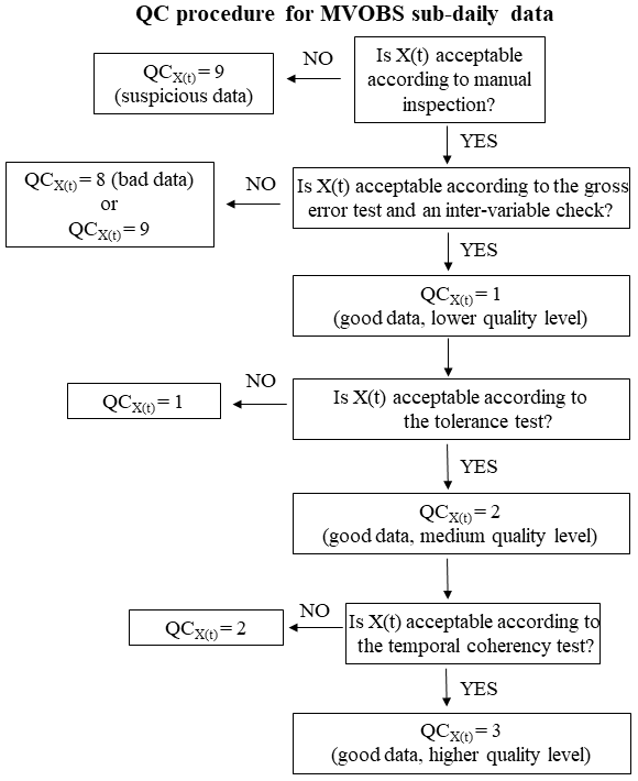
Figure 5A schematic of the QC strategy developed in this study to check the observation of a determined parameter X collected at the time t. It should be highlighted that the cloud cover parameter underwent only the gross error test, and the temporal coherency test has not been applied to precipitation data (accumulated rainfall and snowfall).
The tolerance and temporal tests require a solid assessment of the climatology of the considered parameter. Therefore, we applied a full QC procedure only to the variables with a high data availability (i.e. at least 30 years of continuous measurements): dry-bulb temperature, wet-bulb temperature, atmospheric pressure, vapour pressure, relative humidity, cloud cover, rainfall and snowfall. For the remaining parameters (i.e. cloud direction, wind direction, wind speed, cloud type, visibility, low-level cloud base height and quantity, snow depth, precipitation duration, and precipitation type), we performed a basic manual inspection check that in the case of wind speed, snow depth and visibility takes into account the acceptable limits suggested by the WMO (2008).
The applied QC process is exclusively based on the self-consistency and internal coherence of the investigated dataset. In the event that other sub-daily time series collected in southern Italy become available in future, additional quality evaluations of MVOBS sub-daily data will be carried out through spatial consistency checks.
Data homogenization is widely recognized to be an important part of climate data processing (e.g. Alexandersson an Moberg, 1997). Potential inhomogeneity in MVOBS sub-daily time series may arise from the change in the instruments' location in 1895 and from a turnover of the personnel responsible for the meteorological observations (see Table 1). However, the scientific community is still looking for robust and widely accepted methods for sub-daily data homogenization (Venema et al., 2012). This aspect is well highlighted in the recent work of Ashcroft et al. (2018), in which the rescued sub-daily data were subjected to a QC procedure that did not include the homogenization.
The following subsections provide details and examples about each of the four QC steps.
3.1 Manual inspection
Quality assurance of the MVOBS sub-daily dataset starts during the digitization process. As outlined in Sect. 2.2, at the end of each rescued month, the values uploaded on digital templates were cross-checked with the ones reported in the original source. Manual inspection provided feedback to the digitizers as well as identified common typing errors and transcription mistakes (e.g. doubling, adding or forgetting a number, omission of negative sign, forgetting decimal separator etc).
This step also allowed a preliminary assessment of data quality, which helped familiarize us with some issues affecting the quality of MVOBS sub-daily data, mainly related to the thermo-psychrometric observations. Specifically, combining visual checking with plots for data display, we were able to identify residual imprecisions in the digitized measurements that could have been difficult to identify through the objective statistical procedures.
Through the visual inspection we were able to identify suspicious T and Tw values (flagged with QC=9) measured from 1920 to 1925 and from 1948 to 1951. In the first period, only even values of the temperature were reported, whereas in the second one only the integer part of T and Tw was transcribed.
Other suspicious values identified are associated with observed hydrometeors and the corresponding measurements of accumulated rainfall or snowfall. In particular, we have examined the coherence between these parameters, and we have found two “anomalous” scenarios. In the first scenario of non-measurable precipitation, a hydrometeor is detected and reported in the meteorological register despite the respective accumulated precipitation values being zero. Those circumstances were easily recognizable because the observer wrote down the occurrence of no measurable precipitation as a textual note. Thus, we did not apply any suspicious or bad-quality flag to such data. In the second scenario, although no hydrometeors were detected, the recorded accumulated precipitation was greater than zero. These measurements accounted for the equivalent in liquid of a snowfall event that occurred the day before the specific sub-daily observation was performed. In this case, the accumulated precipitation was measured from the melting of the snow accumulated in the rain gauge, and in the absence of rain gauge heating this process may take a relatively long time, causing an inconsistency between type and accumulated precipitation measurements. To address this issue, we performed a manual correction by aligning in time the occurrence of a certain snowfall event and the respective ELP value. In some cases, the latter refers to the whole snowfall event (that may span a period that includes two or three sub-daily observations and, very occasionally, a period greater than 24 h); therefore we were not able to retrieve the sub-daily values.
3.2 Statistical tests
As already mentioned, after manual inspection, the digitized sub-daily data went through three different statistical procedures. The gross error test is the first check and consists of comparing the investigated sub-daily values to their physical limits. This check gives a relevant contribution to the quality assurance of the climatological dataset by identifying and discarding clearly erroneous values (Baker, 1992; Feng et al., 2004).
Table 2 lists the upper and lower limits considered for each of the tested meteorological parameters. These limits have been chosen following WMO (2008) suggestions. These suggestions contain detailed information on the physical boundaries of several variables. Data that have passed the gross error test have been labelled as QC=1; otherwise they have been labelled as bad data (QC=8). This QC step also includes an inter-variable check aimed to detect and flag inconsistencies between physically related meteorological variables such as T and Tw. In particular, we searched for cases where Tw>T and flagged these as suspicious data (QC=9).
Table 2For each meteorological parameter, upper and lower physical limits used in gross error test are listed.

The second statistical procedure is the tolerance test, which aims to detect the outliers defined as extreme values that exceed climatological limits. The tolerance test has been applied only to sub-daily observations that have passed the manual inspection and the gross error test. In this case, the observation of a certain parameter has been compared to the reference statistical distribution model, computed on a monthly basis (i.e. considering all sub-daily observations collected in a specific month during the investigated period, 1884–1963). It should be noted that cloud cover data did not undergo tolerance and temporal coherence tests. The cloud amount was estimated by visual observations using a fixed reference scale. Due to the specific nature of this parameter and its strong hour-to-hour variability, it is not possible to define climatological limits for outlier and anomalous jump detection. Therefore, quality control for cloud cover includes only manual inspection and the gross error test, and it aims to assess the data plausibility and their consistency with other related meteorological parameters such as cloud type and, when available, low-level cloud base height and quantity.
Depending on the nature of the considered meteorological parameter, we used a different statistical distribution model to assess the climatological limits. Specifically, for variables whose distribution can be fitted by a Gaussian model (i.e. dry- and wet-bulb temperature, atmospheric pressure, and water vapour), an observation X collected at the time t has been flagged as an outlier if one of the following inequalities was verified:
and
where σ and μ are the reference standard deviation and mean for a specific month. As an example, Fig. 6a shows the histogram of the mean January sub-daily dry-bulb temperature from 1884 to 1963. This distribution has been easily modelled through the Gaussian probability density function (red curve). Black vertical lines indicate the lower and upper climatological limits (−9.7 and 10.5 ∘C, respectively) obtained by applying the criteria (3σ-μ) and (3σ+μ), with σ=3.4 ∘C and μ=0.4 ∘C.
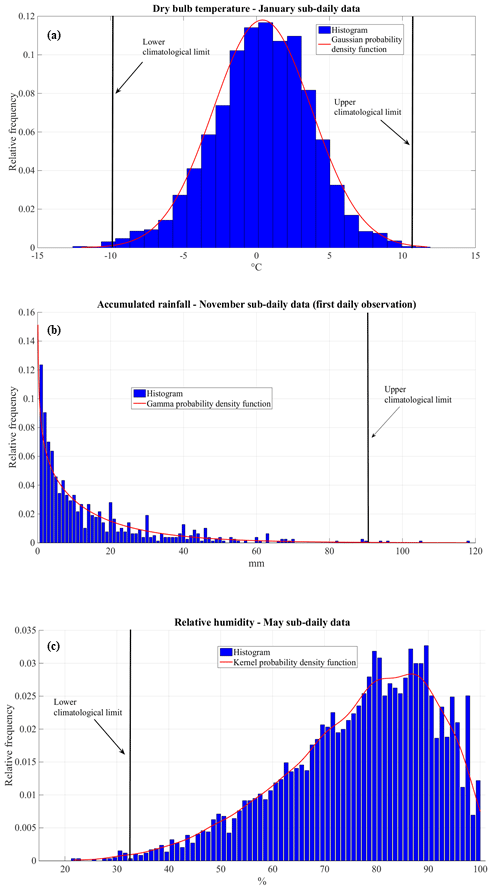
Figure 6Examples of probability distribution models designed within the framework of the tolerance test. Panel (a) shows the Gaussian probability density function applied to dry-bulb temperature collected in January, panel (b) the gamma distribution density function used to model accumulated rainfall data measured in November and panel (c) the kernel density function applied to relative humidity records collected in May. Vertical black lines indicate the tolerance limits fixed using the criteria expressed from Eqs. (5), (6), (7) and (8).
In order to represent the sub-daily precipitation data (accumulated rainfall and snowfall) distribution, we employed the gamma function. This function is well suited for positively skewed variables (such as rainfall), as widely is recognized in the literature (Wilks, 1989; Husak et al., 2007). As already described in Sect. 2.1, the sub-daily meteorological observations performed at MVOBS were not equally spaced over time. Therefore, for time-integrated variables such as precipitation, an adequate pre-processing has been applied to obtain a fair evaluation of their quality. Specifically, before undergoing the tolerance test, rainfall and snowfall data were each divided into two time series. The first time series includes the earliest observation of each day collected at 09:00 or 08:00 local time since 1933 and consists of accumulated precipitation data at a 12 or 13 h' time interval, respectively. The second time series encompasses the second and third observations of every day measured at 15:00 and 21:00 local time from 1884 to 1932 as well as at 14:00 and 19:00 local time since 1933, reporting the accumulated precipitation at a smaller time interval of 5 or 6 h. The frequency distribution of the two time series has been fitted on a monthly basis to a gamma distribution after estimating the shape and scale parameters (e.g. Hubbard et al., 2012).
The criterion used to classify a specific precipitation measure Xt as outlier can be written as follows:
where TPR is the sub-daily precipitation threshold calculated from the gamma distribution for a given probability p (Hubbard et al., 2012). The latter can be interpreted as the probability that the variable takes a value less than or equal to TPR according to the gamma distribution. In this work, we are interested in flagging the anomalous precipitation events (values that are above the climatological limit), so we considered p=0.995 for both rainfall and snowfall sub-daily data. Figure 6b shows the frequency distribution of the mean accumulated November rainfall (for the first observation of the day) collected from 1884 to 1963. A gamma probability density function has been applied to assess an upper climatological limit (91.2 mm in this case). Sub-daily values that exceeded such a threshold have been classified as outliers.
The MVOBS relative humidity data distribution is strongly skewed and therefore is not adequately described by the classic parametric distribution typically employed in the meteorological field such as Gaussian, gamma or generalized Pareto. Therefore, we used a non-parametric kernel density function to model hygrometric measurements. We applied this estimator to the monthly relative humidity distributions using a Gaussian kernel as a smoothing function (Wilks, 2006). The threshold for outlier detection has been assessed through the same approach previously described for the precipitation data. However, in this case we are interested in finding the lower climatologic limit; therefore a determined relative humidity observation has been flagged as an outlier if
where TRH is the threshold of sub-daily relative humidity for a given probability p (=0.005), computed using kernel density distribution. An example of relative humidity frequency distribution modelling is provided by Fig. 6c, which shows the histogram of sub-daily relative humidity observations for May and the associated kernel probability density function (red curve). This allowed the lower climatological limit (32 %), depicted as vertical black line, to be fixed.
To summarize: a sub-daily data point that meets (depending on its frequency distribution model) one of the criteria expressed by Eqs. (5), (6), (7) and (8) has been flagged as an outlier, and therefore its QC value remains at the lowest level (QC=1); otherwise, it has been labelled as QC=2.
Sub-daily data that have passed gross and tolerance tests (QC=2) were subjected to the final QC procedure: the temporal coherency test. The third statistical test, as the previous two, is considered a fundamental part of any QC procedure (Fiebrich and Crawford, 2001; Steinacker et al., 2011). This check is particularly suitable for high-temporal-resolution weather data because the correlation degree between time-adjacent samples increases with the sampling rate.
In this work, we applied the temporal coherency test to detect implausible change between instantaneous sub-daily values collected at two consecutive times. Accumulated rainfall and snowfall data, being time-integrated values, were not analysed in terms of plausible rate of change, so for those parameters the highest-quality flag is QC=2.
The rate of change between two successive measurements of a certain parameter has been compared against a maximum climatological gradient (Δmax). The latter has been determined in the following manner: in the first stage, we computed the first derivative of the investigated time series and subsequently determined the frequency distribution of two different subsets on monthly basis: one including only the differences between observations separated by 12 or 13 h and the other consisting of differences between data separated in time by 5 or 6 h. For all the considered meteorological parameters (dry- and wet-bulb temperature, atmospheric pressure, relative humidity, and vapour pressure), the histograms can be modelled using a Gaussian probability density function. Therefore, after retrieving the histogram mean (μΔ) and standard deviation (σΔ), we fixed Δmax = : if the rate of change between two consecutive observations (as an example, lies between such limits, then QC=3 has been assigned to the record Xt+1.
Figure 7 shows the sub-daily relative humidity observations collected in March 1901. Each data point is colour-coded according to the label assigned by the QC procedure just described. Rates of change in hygrometric conditions that exceed the maximum climatological gradient assessed for March were detected on 6 March at 09:00 and 15:00 local time. In the first case, the difference to the previous observation (5 March, 21:00 local time), 49.9 %, was greater than Δmax found for 12 h observations (39.9 %), whereas in the second one the difference to prior record, equal to 42 %, was above the climatological limit discovered for 6 h data (35.5 %). Both observations were tagged as QC=2 (red dots). It should also be highlighted that three records go beyond the upper RH physical limit (RH=100 %). Such observations were flagged as QC=8 and are indicated as magenta dots. The remaining data have passed all statistical tests (gross, tolerance and temporal coherency), and they have been labelled as QC=3 (green dots).
3.3 Effects of quality control procedure
Table 3 shows the results of the QC procedure applied to MVOBS sub-daily meteorological data. Among the five variables subjected to a full QC, atmospheric pressure is the one with the highest number of values flagged with QC=3 (98.3 %). For this parameter, no bad or suspicious data were recorded. The other four variables (dry- and wet-bulb temperature, relative humidity, and vapour pressure) exhibit similar percentages among different QC levels. Specifically, thermometric measurements have a slightly higher percentage of QC=3 values, but at the same time they show a larger amount of suspicious data after manual inspection (QC=9). Bad data, i.e. values that exceed acceptable physical limits, have been detected only for two parameters: vapour pressure (0.4 %) and relative humidity (0.3 %). The amount of data that do not reach the higher QC=3 level is generally less than 2 %.
Table 3Results of quality control tests applied to MVOBS sub-daily meteorological data. Each column shows the percentage of data flagged as QC=8; QC=9; QC=1; QC=2; and QC=3. It should be noted that cloud cover data underwent only manual inspection and the gross error test, whereas rainfall and snowfall measurement quality was evaluated according to manual inspection as well as the gross error and tolerance tests.

Cloud cover and precipitation only went through the first and second statistical test, respectively. For these parameters, we obtained very good results from the QC analysis. However, for cloud cover we were only able to check the plausibility of data measured with an empirical approach and for such reason subject to subtle inhomogeneity and bias caused by changes in personnel involved in the meteorological observations.
Figure 8a provides compelling evidence of the QC results for the parameters (i.e. dry- and wet-bulb temperature, atmospheric pressure, vapour pressure and relative humidity) that completed the procedure. The figure shows the distribution over time, computed over a 5-year period, of the percentage of sub-daily data whose quality level does not achieve the best value (QC=3). The number of sub-daily values that did not satisfy all steps of the QC procedure is generally less than 3 % except in the time segments 1919–1923 (64.8 %), 1924–1928 (33.1 %), 1944–1948 (17.1 %) and 1949–1953 (58.2 %). It can be noted that a large part of sub-daily data collected in those periods have been flagged as QC=9 after visual inspection. The depletion of data quality detected in the above-mentioned sub-periods is mainly caused by human error, as already discussed in Sect. 3.1, and in particular by imprecisions in thermo-psychrometric measurements. These imprecisions also had a negative impact on the vapour pressure and relative humidity data quality and therefore contribute to a substantial increase in the overall percentage of records flagged as QC=9. Panels (b) and (c) of Fig. 8 show the frequency distribution of dry-bulb temperature in the 1919–1925 and 1948–1950 periods, respectively, providing insight of the inaccuracies in thermos-psychrometric observations found by visual inspection of digitized data. In Fig. 8b, it can be clearly seen that even temperature values have an absolute frequency that is much higher than odd ones. The histogram in Fig. 8c, which only shows temperature records between 10 and 20 ∘C, highlights an anomalous high frequency in the integer temperature values recorded.
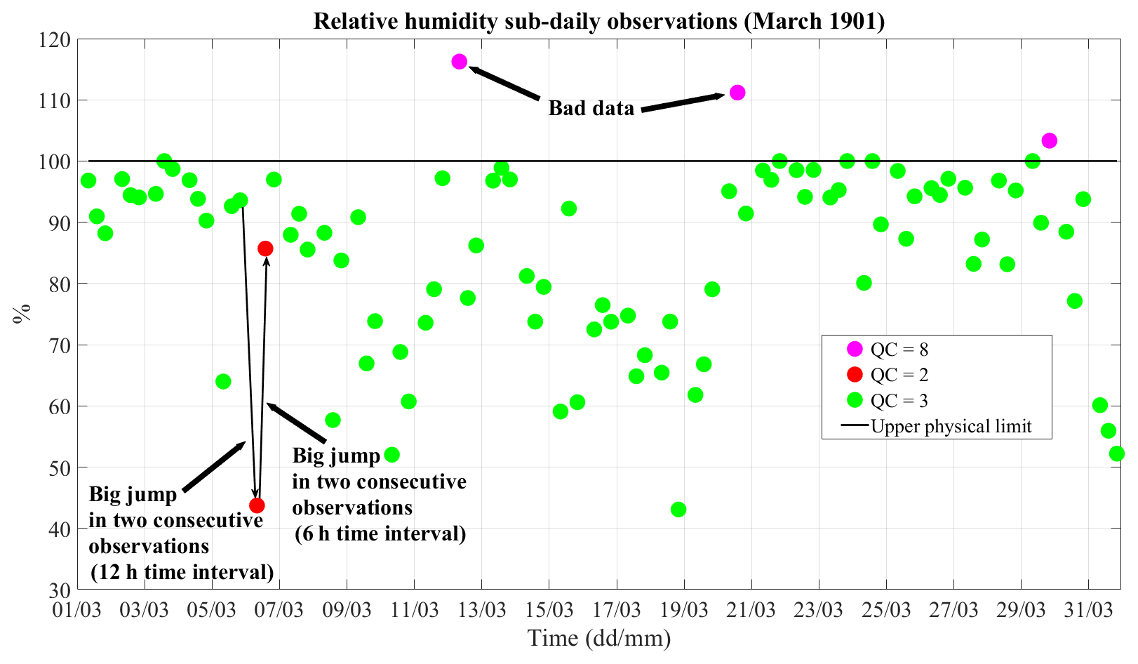
Figure 7Relative humidity (in %) sub-daily observations collected in March 1901. Each record is colour-coded according to its quality flag: bad data (QC=8; magenta), good data with a medium quality level (QC=2; red) and good data with a higher quality level (QC=3; green). In this example, no good data with a lower quality level (QC=1) or suspicious data (QC=9) were detected. The horizontal black line shows the upper physical limit.
This result demonstrates that visual inspection is an essential part of the QC strategy, highlighting some impairments in data quality (mainly caused by human errors) that would otherwise be very difficult to flag through automatic statistical methods.
Rescued and quality-controlled historical sub-daily data play an invaluable role in many research projects and initiatives focused on the comprehension of climate dynamics and on the identification and analysis of past event severity and frequency (WMO, 2016). However, the traceability of long-term and quality-controlled sub-daily records is currently very poor in the Mediterranean area despite the fact that meteorological conditions have been regularly and thoroughly monitored since 19th century (Brunet et al., 2014b). This deficiency exerts a large negative impact not only on studies focused on climate change and variability but also on initiatives intended to develop socio-economic adaptation strategies. It is a fact that such political actions are based on the robustness and accuracy of climate models and reanalysis products, which result in turn from high-quality rescued historical climatic time series.
The recovered data presented in this study offer the first available database in the central and northern Mediterranean region to present sub-daily variability of meteorological parameters for a period ranging from the late 19th century to the early 1960s. The relevance of MVOBS data is also emphasized by the peculiar geographic context in which they have been collected (Apennine region). Therefore, this dataset offers a new opportunity to reconstruct and characterize past climate and weather event dynamics in high-altitude environments, which are notoriously strongly sensitive to climate change.
In this section, we present some possible uses of the MVOBS sub-daily observations from both a meteorological and climatological point of view. In Sect. 4.1 we focus on the evidence of a remarkable past cold-wave event in the MVOBS data, and in Sect. 4.2 we show the potential use of MVOSB data to analyse the long-term atmospheric variability. It is important to note that, at this stage, sub-daily MVOBS data do not allow the performance of a solid climatological analysis because they have not been homogenized. For this reason, Sect. 4.2 only aims to show, from a qualitative perspective, some possible future applications of MVOBS sub-daily records in climate fields with a particular emphasis on some meteorological parameters whose historical variability is largely unknown.
4.1 February 1956 cold wave
Figure 9 shows the behaviour of sub-daily meteorological data collected at MVOBS in February 1956. During this period, a strong cold wave affected Central and Western Europe as well as many regions of the Mediterranean area, causing a large number of fatalities and great plant damage (Dizerens et al., 2017). Twardosz et al. (2016) give an idea of the relevance of such an event: they observe temperature anomalies with respect to the climatological average ranging from −8 to −11 ∘C in most of Europe.

Figure 8In panel (a), colour-coded bars indicate the distribution over time, computed for a 5-year period, of the percentage of sub-daily data that did not pass the full QC procedure: QC=8 (blue); QC=9 (orange); QC=1 (green); and QC=2 (magenta). Panels (b) and (c) present the frequency distribution of dry-bulb temperature in the periods 1919–1925 and 1948–1950, respectively. It should be noticed that panel (c) only shows temperature values between 10 and 20 ∘C. The bin width is 1.0 ∘C in panel (b) and 0.2 ∘C in panel (c).
Figure 9a presents the evolution of atmospheric pressure (red) and dry-bulb temperature (blue) from 1 to 23 February. The air temperature was always below 0 ∘C. The cold wave became particularly severe from day 3 to 9 and between day 15 and 18, when average temperatures of −8.4 and −8.0 ∘C were observed, respectively.
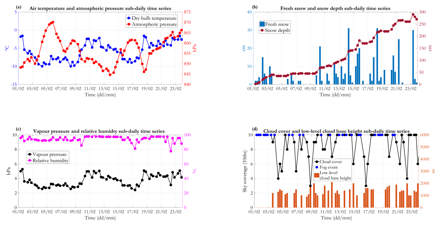
Figure 9Sub-daily time series of different meteorological parameters observed from 1 to 23 February 1956. Panel (a) shows the dry-bulb temperature and atmospheric pressure. Panel (b) presents the fresh snow and snow depth records. Panel (c) shows vapour pressure and relative humidity. Panel (d) plots the cloud cover and low-level cloud base height observations. It should be noticed that such data were subject to a quality control procedure that did not include the homogenization.
The atmospheric pressure was relatively high due to the advection of continental arctic air mass. A drop in pressure was registered between day 10 and 13, when the cold air interacted with moister and warmer Mediterranean air, causing a large amount of snow precipitation as shown in the Fig. 9b from the accumulated fresh snow and the snow depth. Snowfall events were recorded in more than half of the total number of sub-daily observations registered in the investigated time interval. Snow depth exhibited a near-continuous positive trend and reached a value just below 300 cm on day 23. Due to the persistence of atmospheric conditions favourable to precipitation events, relative humidity (Fig. 9c, magenta line) was generally higher than 90 %. Water vapour pressure values (in black), ranging from 3 to 5 hPa, emphasize the occurrence of conditions closer to saturation.
Figure 9d supplies a further example of meteorological sub-daily data collected at MVOBS during February 1956, showing useful information about cloud cover (in black) and low-level cloud base height (vertical orange bars).
Fog conditions that make a reliable evaluation of cloud type and base altitude impossible are marked as blue dots.
The qualitative description of these data and their assimilation in large-scale datasets can be useful to global and regional reanalysis products, which in some cases and in determined regions do not have adequate input to properly reproduce the dynamics of past meteorological events. In this sense, a relevant example dealing with the February 1956 cold wave is provided by the work of Dizerens et al. (2017), who present the observations assimilated by 20CR version 2c for 1 February 1956 (12:00 UTC). According to Compo et al. (2011), the 20CR version 2c reanalysis dataset covers a period spanning from 1871 to 2010.
In the central Mediterranean region, data availability on 1 February is scarce and restricted to northern Italy and to the coastal areas of southern Italy and northern Africa. Strong efforts are then needed to fill these consistent gaps. The dataset rescued in our work can certainly give a significant contribution in this direction, providing unique and rare information on February 1956 cold-wave effects on the Apennine Mountains as well as on the thermos-hygrometric conditions near the 850 hPa isobaric surface, which is usually used for air mass identification.
4.2 Pressure and hail event long-term variability
MVOBS sub-daily data, covering a time interval of 80 years (with some minor gaps), can be helpful for the reconstruction of the variability and trend of the climate in the first half of the 20th century. Specifically, the rescued data can strengthen the current knowledge of the fluctuations over time of both the more studied atmospheric variables, such as air temperature, accumulated rainfall and atmospheric pressure, and the less analysed variables, i.e. relative humidity, vapour pressure, precipitation type and accumulated snowfall.
Figure 10 shows the temporal evolution from 1884 to 1963 of the winter atmospheric pressure (Fig. 10a) and of the yearly hail event frequency (Fig. 10b) that can help in evaluating the climatological significance of MVOBS sub-daily observations. The first time series has been obtained by averaging the sub-daily pressure records collected in the winter season (defined in this study as January–February–March) for each year, whereas the second one has been retrieved using the precipitation type information, counting for each year the days on which at least one observation reported a hail event. To highlight the inter-annual and decadal variability from a qualitative perspective, a locally weighted scatterplot smoothing (LOWESS; red curve) with a span of 10 years has been applied. It should be noted that the displayed time series were not homogenized, and therefore they may contain break points and artefacts.
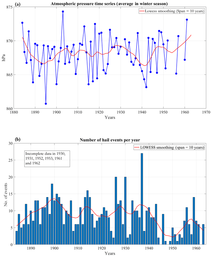
Figure 10Panel (a): time series (blue line) of winter atmospheric pressure from 1884 to 1963. Each value (blue dot) is the average of the sub-daily observations measured during January, February and March. The red curve is the LOWESS filter, computed using a 10-year span. Panel (b): time series (vertical blue bar) of yearly hail events at MVOBS from 1884 to 1963. The hail occurrence has been computed for every year of the investigated period using the sub-daily observations of precipitation type. The red curve is the LOWESS filter, computed using a 10-year span. It should be noted that such data were subject to a quality control procedure that did not include the homogenization.
Atmospheric pressure data collected at MVOBS are useful to complement and extend the historical sub-daily dataset in southern Italy, which includes observations rescued at four different sites (Fig. 1a). The data from these stations cover the 1895–1940 period and are available, in digital format, with a temporal resolution that is lower than the MVOBS dataset; consequently, they totally miss the sub-daily variability of atmospheric parameters. MVOBS can shed more light on past variability of atmospheric pressure in the Mediterranean area and can contribute to the evaluation of its relationship with large-scale atmospheric patterns.
Hail frequency occurrence data offer a great opportunity to build a climatology of hail precipitation, which is gaining more attention due to its severe impacts on crops, properties and buildings (e.g. Santos and Belo-Pereira, 2019). With few exceptions, solid and long-term information about hail incidence has only been available in recent decades (e.g. Zhang et al., 2008; Mezher et al., 2012; Baldi et al., 2014; Santos and Belo-Pereira, 2019) and are often subjected to biases due to the different data sources (weather station, insurance companies, newspapers etc.) used for their reconstruction. The problem of missing data is even greater in some countries, such as Italy (Baldi et al., 2014), where the very limited extension of the observational network seriously compromises the development of a reliable national hail climatology. In this context, the historical and continuous precipitation type observations performed at MVOBS can supply a relevant contribution to the assessment of past variability of hailfall and of the synoptic and local-scale factors that promote the formation of such hydrometeors within convective systems.
The digitized and quality-controlled MVOBS dataset is available through the NOAA's NCEI historical weather data repository. Two different versions of the dataset are provided in Microsoft Excel format. The first one, “Sub_daily_data_MVOBS_raw”, includes all the observed parameters without any quality control information, and the other one, “Sub_daily_MVOBS_QC_VARIABLES”, includes data from all the parameters that have been subjected to statistical quality control tests. Data can be accessed via HTTP using the following website: https://www.nodc.noaa.gov/cgi-bin/OAS/prd/accession/download/205785 (NCEI, 2020). They are also associated with a DOI: https://doi.org/10.25921/cx3g-rj98 (Capozzi et al., 2019).
Rescued and quality-controlled historical datasets play an invaluable role in many research projects and initiatives focused on the comprehension of climate dynamics and on the identification and analysis of past weather event severity and frequency (WMO, 2016). The range of applications of this kind of data encompasses many fields and studies and also concerns the socio-economic impacts of climate change, hydrology and agricultural planning.
This paper presents the rescue and quality control of sub-daily meteorological observations performed at Montevergine Observatory. The data cover a period spanning from 1884 to 1963 and consist of several variables that provide a complete characterization of the atmospheric state in terms of thermodynamic conditions (dry- and wet-bulb temperature, atmospheric pressure, vapour pressure, and relative humidity), precipitation type and amount (accumulated snowfall and rainfall), and sky conditions (cloud cover and type) three times per day. Sub-daily observations and metadata have been recovered from original hand-written registers preserved in the Montevergine abbey bibliographic archive, formatted according to the rules of the Italian Central Office and from old diaries that trace the observatory history. The first step of our work consisted of examining such historic documents to retrieve useful information about the observatory practices, instrument relocation and replacement, change in personnel, and data availability. The meteorological records have been digitized using a simple “key entry” approach, which ensures high quality standards despite being the most time-consuming among the suggested methods by the WMO.
Once digitized, sub-daily data have been quality-controlled using a procedure based on the internal consistency and coherence of the dataset, structured into four different stages: manual inspection, gross error test, tolerance test and temporal coherency test. The percentage of observations that satisfy the entire QC chain ranges from 84 % to 98 %, depending on the considered meteorological variable. Lower data quality (except for atmospheric pressure) have been detected in two time intervals (1920–1925 and 1948–1951) thanks to the manual inspection that highlighted suspicious data due to human imprecision. Among the analysed variables, the thermo-psychrometric records proved to be more susceptible to errors and inconsistencies. This result should not be surprising considering the many sources of errors that affect psychrometric measurements (WMO, 2008), which are mainly related to insufficient ventilation and excessive covering of ice on the wet bulb (an issue that may be particularly common at the high-altitude mountainous site).
The scientific community can use the recovered dataset for many purposes, embracing both meteorological and climatological frameworks. This is due to some peculiar features that are uncommon for long and old climatological time series such as the high time resolution of the weather observations, the variety of recorded meteorological parameters and the uniqueness of the geographical context (southern Apennine Mountains). In the last part of our work, we present two possible uses of MVOBS data related to the detailed characterization of a severe past weather event (February 1956 cold wave) and to the reconstruction of the variability and trend of winter atmospheric pressure and yearly hail event frequency.
This work makes available to scientists an old sub-daily climatological dataset for future employment in research activities after its digitization and quality control. In our opinion, more efforts and actions should be designed to recover and valorize old sub-daily records, especially in Italian territory, which has an inestimable asset of historical meteorological observations. An increase in sub-daily data availability can bring benefits both in terms of quality control and homogenization, allowing procedures relying on spatial consistency and coherence to be devised.
In this sense, one of our future aims is to extend the work performed for MVOBS to other ancient observatories of central and southern Italy. A primary target of this future research may be the Campania region in the southern part of Italy. This region has a vivid and rich heritage of past weather data, in large part still unexplored due to the near-continuous activity of some meteorological specola including, beside MVOBS, the San Marcellino observatory (Naples; established in 1860), the Naples Capodimonte astronomical observatory (inaugurated in 1821) and the Scuola Agraria meteorological observatory in Portici (founded in 1898).
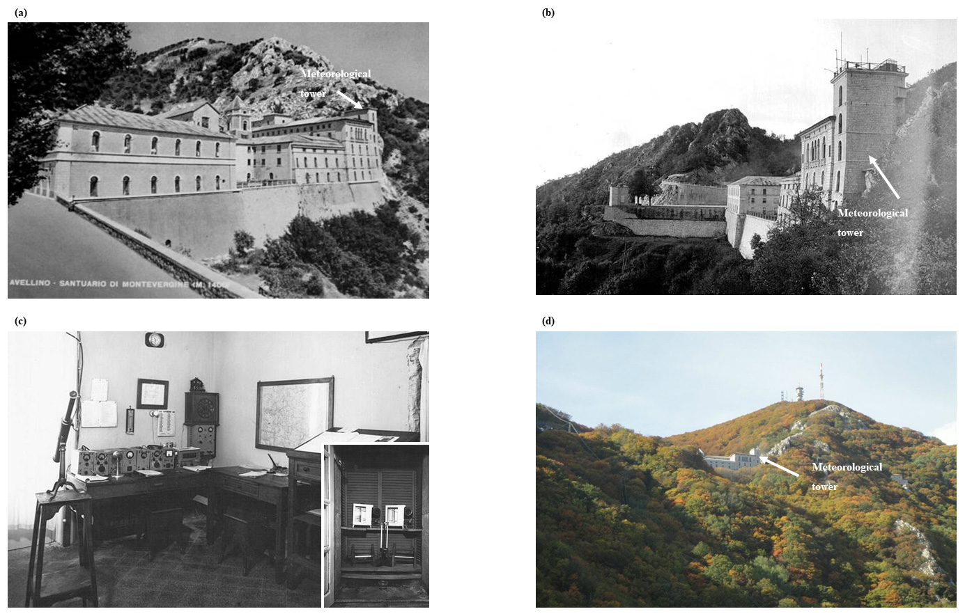
Figure A1Panels (a) and (b): historical view of the MVOBS meteorological tower from a south-eastern and a northern direction, respectively. Panel (c): the observatory room in 1950. The small picture in the bottom right corner of the panel shows the inside of a Stevenson screen, where thermometric and hygrometric measurements were performed. Panel (d): a recent panoramic view of the Montevergine abbey and MVOBS. Historical and recent images show that MVOBS is surrounded by a natural high-altitude environment, whose features have remained unchanged over time. Photos in panels (a), (b) and (c) are courtesy of the Italian Air Force (http://www.meteoam.it/page/montevergine, last access: 25 April 2020).
VC managed the first two steps of the MVOBS data rescue: he analysed the old documents and diaries for metadata retrieval and digitized the entire sub-daily dataset. CDV analysed the MVOBS data availability. YC, PC and VC performed the manual checking of digitized data. YC, VC, PC and CDV designed and applied the statistical test of the quality control procedure. VC wrote the manuscript with contributions from YC, PC, GB and CDV. GB was the coordinator of the EPIMETEO project, which provided the funding for this research, and supervised the entire work.
The authors declare that they have no conflict of interest.
The authors of this work are very grateful to the Benedectine Community of Montevergine for affording the opportunity to analyse and digitize the old diaries and meteorological registers stored in the Montevergine abbey. In this respect, we address special thanks to Reverend Father Abbot Riccardo Guariglia and to Father Benedetto Komar, the current MVOBS director. Moreover, we are grateful to the Italian Air Force for granting the permission to reproduce some old photos of Montevergine Observatory in this paper.
This research has been supported by the EPIMETEO project “Sviluppo e applicazione di nuove metodologie per l'analisi di dati meteorologici acquisiti con tecniche tradizionali e innovative” (grant no. DSTE 330).
This paper was edited by Kirsten Elger and reviewed by Maria Carmen Beltrano and Alba Gilabert Gallart.
Abeli, T., Rossi, G., Gentili, R., Gandini, M., Mondoni, A., and Cristofanelli, P.: Effect of the extreme summer heat waves on isolated populations of two orophitic plants in the north Apennines (Italy), Nord. J. Bot., 30, 109–115, https://doi.org/10.1111/j.1756-1051.2011.01303.x, 2012.
Alexandersson, H. and Moberg, A.: Homogenization of Swedish temperature data. Part I: homogeneity test for linear trends, Int. J. Climatol., 17, 25–34, https://doi.org/10.1002/(SICI)1097-0088(199701)17:1<25::AID-JOC103>3.0.CO;2-J, 1997.
Allan, R., Brohan, P., Compo, G. P., Stone, R., Luterbacher, J., Brönnimann, S., Allan, R., Brohan, P., Compo, G. P., Stone, R., Luterbacher, J., and Brönnimann, S.: The International Atmospheric Circulation Reconstructions over the Earth (ACRE) Initiative, B. Am. Meteorol. Soc., 92, 1421–1425, https://doi.org/10.1175/2011BAMS3218.1, 2011.
Ashcroft, L., Coll, J. R., Gilabert, A., Domonkos, P., Brunet, M., Aguilar, E., Castella, M., Sigro, J., Harris, I., Unden, P., and Jones, P.: A rescued dataset of sub-daily meteorological observations for Europe and the southern Mediterranean region, 1877–2012, Earth Syst. Sci. Data, 10, 1613–1635, https://doi.org/10.5194/essd-10-1613-2018, 2018.
Auer, I., Böhm, R., Jurkovic, A., Lipa, W., Orlik, A., Potzmann, R., Schöner, W., Ungersböck, M., Matulla, C., Briffa, K., Jones, P., Efthymiadis, D., Brunetti, M., Nanni, T., Maugeri, M., Mercalli, L., Mestre, O., Moisselin, J.-M., Begert, M., MüllerWestermeier, G., Kveton, V., Bochnicek, O., Stastny, P., Lapin, M., Szalai, S., Szentimrey, T., Cegnar, T., Dolinar, M., Gajic-Capka, M., Zaninovic, K., Majstorovic, Z., and Nieplova, E.: HISTALP – historical instrumental climatological surface time series of the Greater Alpine Region, Int. J. Climatol., 27, 17–46, https://doi.org/10.1002/joc.1377, 2007.
Baker, N. L.: Quality control for the navy operational atmospheric database. Weather Forecast., 7, 250–261, https://doi.org/10.1175/1520-0434(1992)007<0250:QCFTNO>2.0.CO;2, 1992.
Baldi, M., Ciardini, V., Dalu, J.D., Filippis, T.D., Maracchi, G., and Dalu, G.: Hail occurrence in Italy: towards a national database and climatology, Atmos. Res., 138, 268–277, https://doi.org/10.1016/j.atmosres.2013.11.012, 2014.
Brombacher W. G., Johnson D. P., and Cross J. L.: Mercury Barometers and Manometers, NBS Mono.8, U.S. Govt. Printing Office, Washington, 1960.
Brönnimann, S., Annis, J., Dann, W., Ewen, T., Grant, A. N., Griesser, T., Krähenmann, S., Mohr, C., Scherer, M., and Vogler, C.: A guide for digitising manuscript climate data, Clim. Past, 2, 137–144, https://doi.org/10.5194/cp-2-137-2006, 2006.
Brunet, M., Gilabert, A., Jones, P., and Efthymiadis, D.: A historical surface climate dataset from station observations in Mediterranean North Africa and Middle East areas, Geosci. Data J., 1, 121–128, https://doi.org/10.1002/gdj3.12, 2014a.
Brunet, M., Jones, P. D., Jourdain, S., Efthymiadis, D., Kerrouche, M., and Boroneant, C.: Data sources for rescuing the rich heritage of Mediterranean historical surface climate data, Geosci. Data J., 1, 61–73, https://doi.org/10.1002/gdj3.4, 2014b.
Brunetti, M., Maugeri, M., Monti, F., and Nanni, T.: Temperature and precipitation variability in Italy in the last two centuries from homogenised instrumental time series, Int. J. Climatol., 26, 345–381, https://doi.org/10.1002/joc.1251, 2006.
Capozzi, V. and Budillon, G.: Time series analyses of climatological records from a high altitude observatory in southern Italy (Montevergine, AV), Proceedings of First Annual Conference “Climate change and its implications on ecosystem and society”, Società Italiana per le Scienze del Clima, Lecce, Italy, 2013.
Capozzi, V. and Budillon, G.: Detection of heat and cold waves in Montevergine time series (1884–2015), Adv. Geosci., 44, 35–51, https://doi.org/10.5194/adgeo-44-35-2017, 2017.
Capozzi, V., Cotroneo, Y., Castagno, P., De Vivo, C., Komar, A., Guariglia, R., and Budillon, G.: Sub-daily meteorological data collected at Montevergine Observatory (Southern Apennines), Italy from 1884-01-01 to 1963-12-31 (NCEI Accession 0205785), NOAA National Centers for Environmental Information, Dataset, https://doi.org/10.25921/cx3g-rj98, 2019.
Capozzi, V., Montopoli, M., Bracci, A., Adirosi, E., Baldini, L., Vulpiani, G., and Budillon, G.: Retrieval of snow precipitation rate from polarimetric X-band radar measurements in Southern Italy Apennine mountains, Atmospheric Research, 236, 15 May 2020, 104796, https://doi.org/10.1016/j.atmosres.2019.104796, 2020.
Compo, G. P., Whitaker, J. S., Sardeshmukh, P. D., Matsui, N., Allan, R. J., Yin, X., Gleason, B. E., Vose, R. S., Rutledge, G., Bessemoulin, P., Brönnimann, S., Brunet, M., Crouthamel, R. I., Grant, A. N., Groisman, P. Y., Jones, P. D., Kruk, M. C., Kruger, A. C., Marshall, G. J., Maugeri, M., Mok, H. Y., Nordli, Ø., Ross, T. F., Trigo, R. M., Wang, X. L., Woodruff, S. D., and Worley, S. J.: The Twentieth Century Reanalysis Project, Q. J. Roy. Meteor. Soc., 137, 1–28, https://doi.org/10.1002/qj.776, 2011.
Compo, G. P., Slivinski, L. C., Whitaker, J. S., Sardeshmukh, P. D., McColl, C., Brohan, P., Allan, R., Yin, X., Vose, R., Spencer, L. J., Ashcroft, L., Bronnimann, S., Brunet, M., Camuffo, D., Cornes, R., Cram, T. A., Crouthamel, R., Dominguez-Castro, F., Freeman, J. E., Gergis, J., Giese, B. S., Hawkins, E., Jones, P. D., Jourdain, S., Kaplan, A., Kennedy, J., Kubota, H., Blancq, F. L., Lee, T., Lorrey, A., Luterbacher, J., Maugeri, M., Mock, C. J., Moore, K., Przybylak, R., Pudmenzky, C., Reason, C., Slonosky, V. C., Tinz, B., Titchner, H., Trewin, B., Valente, M. A., Wang, X. L., Wilkinson, C., Wood, K., and Wyszynski, P.: The International Surface Pressure Databank version 4. Research Data Archive at the National Center for Atmospheric Research, Computational and Information Systems Laboratory, https://doi.org/10.5065/9EYR-TY90, 2019.
Cram, T. A., Compo, G. P., Yin, X., Allan, R. J., McColl, C., Vose, R. S., Whitaker, J. S., Matsui, N., Ashcroft, L., Auchmann, R., Bessemoulin, P., Brandsma, T., Brohan, P., Brunet, M., Comeaux, J., Crouthamel, R., Gleason, B. E., Groisman, P. Y., Hersbach, H., Jones, P. D., Jónsson, T., Jourdain, S., Kelly, G., Knapp, K. R., Kruger, A., Kubota, H., Lentini, G., Lorrey, A., Lott, N., Lubker, S. J., Luterbacher, J., Marshall, G. J., Maugeri, M., Mock, C. J., Mok, H. Y., Nordli, Ø., Rodwell, M. J., Ross, T. F., Schuster, D., Srnec, L., Valente, M. A., Vizi, Z., Wang, X. L., Westcott, N., Woollen, J. S., and Worley, S. J.: The international surface pressure databank version 2. Geosci. Data J., 2, 31–46, https://doi.org/10.1002/gdj3.25, 2015.
Diodato, N.: Nota climatica ispirata alla serie storica delle precipitazioni osservate al Santuario di Montevergine, Rivista di Meteorologia Aeronautica, LII-N.34, 179–182, July–December, 1992.
Dizerens, C., Lenggenhager, S., Schwander, M., Buck, A., and Foffa, S.: The 1956 Cold Wave in Western Europe, edited by: Brönnimann, S., Historical Weather Extremes in Reanalyses, Geographica Bernensia, G92, 101–111, https://doi.org/10.4480/GB2017.G92.09, 2017.
Egli, L.: Spatial variability of new snow amounts derived from a dense network of Alpine automatic stations, Ann. Glaciol., 49, 51–55, https://doi.org/10.3189/172756408787814843, 2008.
Egli, L., Jonas, T., and Meister, R.: Comparison of different automatic methods for estimating snow water equivalent, Cold Reg. Sci. Technol., 57, 107–115, https://doi.org/10.1016/j.coldregions.2009.02.008, 2009.
Feng, S., Hu, Q., and Qian, W.: Quality control of daily meteorological data in China, 1951–2000: A new dataset, Int. J. Climatol., 24, 853–870, https://doi.org/10.1002/joc.1047, 2004.
Fiebrich, C. A. and Crawford, K. C.: The Impact of Unique Meteorological Phenomena Detected by the Oklahoma Mesonet and ARS Micronet on Automated Quality Control, B. Am. Meteorol. Soc., 82, 2173–2188, https://doi.org/10.1175/1520-0477(2001)082<2173:TIOUMP>2.3.CO;2, 2001.
Hubbard, K., You, J., and Shulski, M.: Toward a Better Quality Control of Weather Data, Practical Concepts of Quality Control, edited by: Saber, M. and Nezhad, F., ISBN: 978-953-51-0887-0, InTech, https://doi.org/10.5772/51632, 2012.
Husak, G. J., Michaelsen, J., and Funk, C.: Use of the gamma distribution to represent monthly rainfall in Africa for drought monitoring applications, Int. J. Climatol. 27, 935–944, https://doi.org/10.1002/joc.1441, 2007.
Jones, P. D., Groisman, P. Ya., Coughlan, M., Plummer, N., Wang, W.-C., and Karl, T. R.: Assessment of urbanization effects in time series of surface air temperature over land, Nature, 347, 169–172, https://doi.org/10.1038/347169a0, 1990.
Libertino, A., Ganora, D., and Claps, P.: Technical note: Space–time analysis of rainfall extremes in Italy: clues from a reconciled dataset, Hydrol. Earth Syst. Sci., 22, 2705–2715, https://doi.org/10.5194/hess-22-2705-2018, 2018.
Maugeri, M., Bellumé, M, Buffoni, L., and Chlistovsky, F.: Reconstruction of daily pressure maps over Italy during some extreme events of the 19th century, Il Nuovo Cimento, 21, 135–147, 1998.
Mezher, R. N., Doyle, M., and Barros, V.: Climatology of hail in Argentina, Atmos. Res., 114, 70–82. https://doi.org/10.1016/j.atmosres.2012.05.020, 2012.
Montevergine: Montevergine, available at: http://www.meteoam.it/page/montevergine, last access: 25 April 2020.
NCEI: Ocean Archive System, files for accession 205785, available at: https://www.nodc.noaa.gov/cgi-bin/OAS/prd/accession/download/205785, last access: 31 January 2020
Santos, J. A. and Belo-Pereira, M.: A comprehensive analysis of hail events in Portugal: Climatology and consistency with atmospheric circulation, Int. J. Climatol., 39, 188–205, https://doi.org/10.1002/joc.5794, 2019.
Slivinski, L. C., Compo, G. P., Whitaker, J. S., Sardeshmukh, P. D., Giese, B. S., McColl, C., Allan, R., Yin, X., Vose, R., Titchner, H., Kennedy, J., Spencer, L.J., Ashcroft, L., Brönnimann, S., Brunet, M., Camuffo, D., Cornes, R., Cram, T.A., Crouthamel, R., Domínguez-Castro, F., Freeman, J. E., Gergis, J., Hawkins, E., Jones, P.D., Jourdain, S., Kaplan, A., Kubota, H., Blancq, F. L., Lee, T., Lorrey, A., Luterbacher, J., Maugeri, M., Mock, C. J., Moore, G. W. K., Przybylak, R., Pudmenzky, C., Reason, C., Slonosky, V. C., Smith, C. A., Tinz, B., Trewin, B., Valente, M. A., Wang, X. L., Wilkinson, C., Wood, K., and Wyszyński, P.: Towards a more reliable historical reanalysis: Improvements for version 3 of the Twentieth Century Reanalysis system, Q. J. Roy. Meteorol. Soc., 145, 2876–2908, https://doi.org/10.1002/qj.3598, 2019.
Steinacker, R., Mayer, D., and Steiner, A.: Data Quality Control Based on Self-Consistency, Mon. Weather Rev., 139, 3974–3991, https://doi.org/10.1175/MWR-D-10-05024.1, 2011.
Stickler, A., Brönnimann, S., Valente, M. A., Bethke, J., Sterin, A., Jourdain, S., Roucaute, E., Vasquez, M. V., Reyes, D. A., Allan, R., and Dee, D.: ERA-CLIM: Historical Surface and Upper-Air Data for Future Reanalyses, B. Am. Meteorol. Soc., 95, 1419–1430, https://doi.org/10.1175/BAMS-D-13-00147.1, 2014.
The International Surfance Pressure Databank version 4, Interactive Station Viewer, available at: https://rda.ucar.edu/datasets/ds132.2/index.html?sstn=17606&spart=exact#stationViewer, last access: 29 January 2020.
Twardosz, R., Kossowska-Cezak, U., and Pełech, S.: Extremely Cold Winter Months in Europe (1951–2010), Acta Geophys., 64, 2609–2629, https://doi.org/10.1515/acgeo-2016-0083, 2016.
Venema, V. K. C., Mestre, O., Aguilar, E., Auer, I., Guijarro, J. A., Domonkos, P., Vertacnik, G., Szentimrey, T., Stepanek, P., Zahradnicek, P., Viarre, J., Müller-Westermeier, G., Lakatos, M., Williams, C. N., Menne, M. J., Lindau, R., Rasol, D., Rustemeier, E., Kolokythas, K., Marinova, T., Andresen, L., Acquaotta, F., Fratianni, S., Cheval, S., Klancar, M., Brunetti, M., Gruber, C., Prohom Duran, M., Likso, T., Esteban, P., and Brandsma, T.: Benchmarking homogenization algorithms for monthly data, Clim. Past, 8, 89–115, https://doi.org/10.5194/cp-8-89-2012, 2012.
Westra, S., Fowler, H. J., Evans, J. P., Alexander, L. V., Berg, P., Johnson, F., Kendon, E. J., Lenderink, G., and Roberts, N. M.: Future changes to the intensity and frequency of short-duration extreme rainfall, Rev. Geophys., 52, 522–555, https://doi.org/10.1002/2014RG000464, 2014.
Wilks, D. S.: Conditioning Stochastic Daily Precipitation Models on Total Monthly Precipitation, Water Resour. Res., 25, 1429–1439, 1989.
Wilks, D. S.: Statistical Methods in Atmospheric Sciences, 2nd ed., Academic Press: Burlington, NJ, USA, 2006.
Winiger, M., Gumpert, M., and Yamout, H.: Karakorum–Hindukush–western Himalaya: assessing high-altitude water resources, Hydrol. Process. 19, 2329–2338, https://doi.org/10.1002/hyp.5887, 2005.
World Meteorological Organization: Guide to Meteorological Instruments and Methods of Observation, 2008 Edition, WMO-no. 8 (Seventh edition), available at: https://www.wmo.int/pages/prog/www/IMOP/publications/CIMO-Guide/OLD-pages/CIMO_Guide-7th_Edition-2008.html (last access: 1 October 2019), 2008.
World Meteorological Organization: Guide to Meteorological Instruments and Methods of Observation, 2014 Edition (updated in 2017), WMO-no. 8, available at: https://www.wmo.int/pages/prog/www/IMOP/CIMO-Guide.html (last access: 15 October 2019), 2014.
World Meteorological Organization: Guidelines on Best Practices for Climate Data Rescue 2016, WMO-No. 1182, available at: https://public.wmo.int/en/resources/library/guidelines-best-practices-climate-data-rescue (last access: 30 September 2019), 2016.
Zhang, C. X., Zhang, Q. H., and Wang, Y. Q.: Climatology of hail in China: 1961–2005, J. Appl. Meteorol. Clim., 47, 795–804, https://doi.org/10.1175/2007JAMC1603.1, 2008.
- Abstract
- Introduction
- Materials, data and methods
- Quality control of digitized data
- Application examples of MVOBS sub-daily dataset
- Data availability
- Conclusions
- Appendix A: Historical and modern views of Montevergine Observatory
- Author contributions
- Competing interests
- Acknowledgements
- Financial support
- Review statement
- References