the Creative Commons Attribution 4.0 License.
the Creative Commons Attribution 4.0 License.
 | 14 Jun 2019
The TRIple-frequency and Polarimetric radar Experiment for improving process observations of winter precipitation
Stefan Kneifel
Davide Ori
Silke Trömel
Jan Handwerker
Birger Bohn
Normen Hermes
Kai Mühlbauer
Martin Lenefer
Clemens Simmer
This paper describes a 2-month dataset of ground-based triple-frequency (X, Ka, and W band) Doppler radar observations during the winter season obtained at the Jülich ObservatorY for Cloud Evolution Core Facility (JOYCE-CF), Germany. All relevant post-processing steps, such as re-gridding and offset and attenuation correction, as well as quality flagging, are described. The dataset contains all necessary information required to recover data at intermediate processing steps for user-specific applications and corrections (https://doi.org/10.5281/zenodo.1341389; Dias Neto et al., 2019). The large number of ice clouds included in the dataset allows for a first statistical analysis of their multifrequency radar signatures. The reflectivity differences quantified by dual-wavelength ratios (DWRs) reveal temperature regimes where aggregation seems to be triggered. Overall, the aggregation signatures found in the triple-frequency space agree with and corroborate conclusions from previous studies. The combination of DWRs with mean Doppler velocity and linear depolarization ratio enables us to distinguish signatures of rimed particles and melting snowflakes. The riming signatures in the DWRs agree well with results found in previous triple-frequency studies. Close to the melting layer, however, we find very large DWRs (up to 20 dB), which have not been reported before. A combined analysis of these extreme DWR with mean Doppler velocity and a linear depolarization ratio allows this signature to be separated, which is most likely related to strong aggregation, from the triple-frequency characteristics of melting particles.
- Article
(7745 KB) - Full-text XML
-
Supplement
(313 KB) - BibTeX
- EndNote


The combined observation of clouds and precipitation at different radar frequencies is used to improve retrievals of hydrometeor properties. All methods exploit frequency-dependent hydrometeor scattering and absorption properties governed by their microphysical characteristics.
Multifrequency retrievals are already well developed for liquid hydrometeors. For example, Hogan et al. (2005) used differential radar attenuation at 35 and 94 GHz to retrieve vertical profiles of cloud liquid water. Improved precipitation rate retrievals on a global scale are provided by the core satellite of the Global Precipitation Mission which operates a Ku–Ka band dual-frequency radar (Hou et al., 2014). For frequencies below ≈10 GHz, attenuation effects are negligible (except for heavy rainfall or hail), and the sensitivity to non-precipitating particles, such as ice crystals, is relatively weak. Therefore, the majority of multifrequency applications for cold clouds focus on cloud radar systems operating at 35 or 94 GHz. At these frequencies, the radars are sensitive enough to detect even sub-millimeter ice particles and cloud droplets. The sizes of large ice crystals, snowflakes, graupel, and hail are on the order of the wavelengths used to observe them (3 mm, 8 mm, and 3 cm for W, Ka, and X band, respectively). Thus, non-Rayleigh scattering becomes important and can be used to constrain particle size distributions, improving ice and snow water content retrievals (Matrosov, 1998; Hogan et al., 2000; Leinonen et al., 2018; Grecu et al., 2018).
Recent modeling studies (Kneifel et al., 2011b; Tyynelä and Chandrasekar, 2014; Leinonen and Moisseev, 2015; Leinonen and Szyrmer, 2015; Gergely et al., 2017) revealed that different ice particle classes like graupel, single crystals, or aggregates can be distinguished using a combination of three radar frequencies (13, 35, and 94 GHz). Triple-frequency radar datasets from airborne campaigns (Leinonen et al., 2012; Kulie et al., 2014) and satellites (Yin et al., 2017) confirmed distinct signatures in the triple-frequency space. Ground-based triple-frequency radar measurements in combination with in situ observations (Kneifel et al., 2015) provided the first experimental evidence for a close relation between triple-frequency signatures and the characteristic particle size, as well as the bulk density of snowfall. These early results were corroborated and refined by coinciding in situ observations in aircraft campaigns (Chase et al., 2018) as well as by ground-based observations (Gergely et al., 2017). A better understanding of the relations between triple-frequency signatures and snowfall properties is key for triple-frequency radar retrieval development. The connection between scattering and microphysical properties is currently addressed by novel ground-based in situ instrumentation (Gergely et al., 2017) and triple-frequency Doppler spectra (Kneifel et al., 2016). Long-term triple-frequency datasets from various sites and radar systems are, however, needed to better understand the relations between triple-frequency signatures and clouds.
We present a first analysis of triple-frequency (X, Ka, and W band) radar observations collected over two winter months at the Jülich Observatory for Cloud Evolution Core Facility, Germany (Löhnert et al., 2015). The data were corrected for known offsets and attenuation effects and re-gridded for multifrequency studies. Section 2 describes the experimental setup and the characteristics of the X, Ka, and W band radars. Section 3 details the data processing and corrections applied. Section 4 gives a general overview of the dataset and its limitations. Section 5 presents a statistical analysis of the data with a focus on the temperature dependency of the triple-frequency properties, signatures of riming, intense aggregation, and melting snow particles. We summarize and discuss our results in Sect. 6.
The TRIple-frequency and Polarimetric radar Experiment for improving process observation of winter precipitation (TRIPEx) was a joint field experiment of the University of Cologne, the University of Bonn, the Karlsruhe Institute of Technology (KIT), and the Jülich Research Centre (Forschungszentrum Jülich, FZJ). TRIPEx took place at the Jülich Observatory for Cloud Evolution Core Facility (JOYCE-CF 50∘54′31′′ N, 6∘24′49′′ E; 111 m above mean sea level) from 11 November 2015 until 4 January 2016. The core instruments deployed during TRIPEx were three vertically pointing radars providing a triple-frequency (X, Ka, and W band) column view of the hydrometeors aloft. All three radars were calibrated by the manufacturers before the campaign. Figure 1 sketches the positions of the instruments relative to each other and the ground surface. A large number of additional permanently installed remote sensing and in situ observing instruments are available at the JOYCE-CF site (see Löhnert et al., 2015, for a detailed overview).
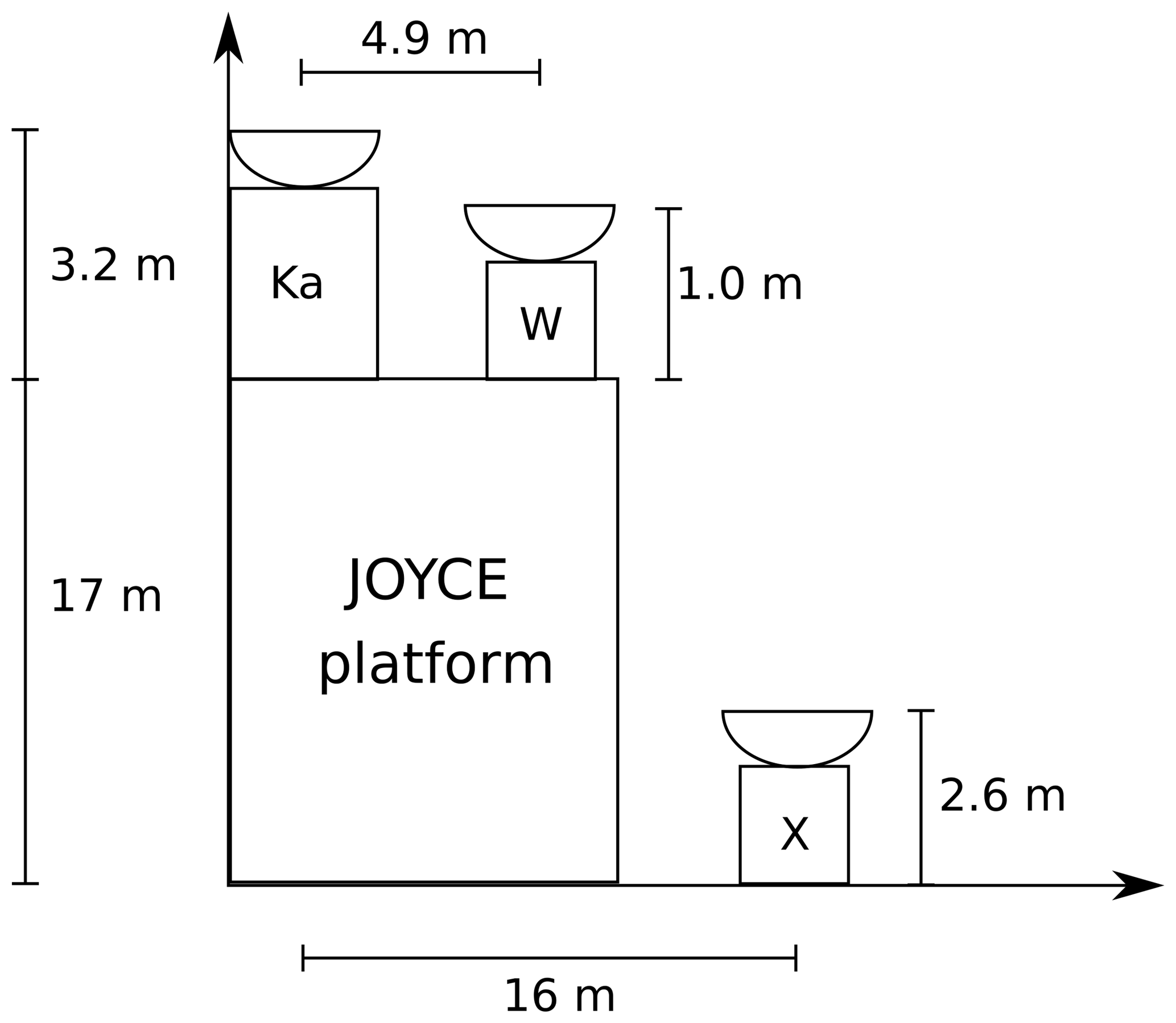
Figure 1Sketch (not to scale) of the horizontal and vertical distances between the three zenith-pointing radars operated during TRIPEx. The JOYCE-CF platform with all auxiliary instruments is located on the roof of a 17 m tall building. The mobile X band radar was placed on the ground close to the other two radars.
2.1 Precipitation radar KiXPol (X band)
KiXPol, hereafter referred to as the X band, is a pulsed 9.4 GHz Doppler precipitation radar, usually integrated into the KITcube platform (Kalthoff et al., 2013). The mobile Meteor 50DX radar, manufactured by Selex ES (Gematronik), is mounted on a trailer and placed next to the JOYCE-CF building in order to position it as close as possible to the other two radars, which were installed on the JOYCE-CF roof platform (see Fig. 1). The radar operates in a simultaneous transmit and receive (STAR) mode and is thus capable of measuring standard polarimetric variables like differential reflectivity Zdr and differential phase shift Φdp. The linear depolarization ratio (LDR) is not provided because it requires the emission of single-polarization pulses in order to allow for independent measurements of the cross-polarized component of the returning signal. During the campaign, the X band was set to a pulse duration of 0.3 µs; a slight oversampling was applied to achieve a radial resolution of 30 m in order to match the resolution of the other radars as close as possible (see Table 1). The X band radar is designed for operational observations of precipitation via volume scans (series of azimuth scans at several fixed elevation angles). KiXPol was operated at JOYCE in this mode during the HOPE campaign (Xie et al., 2016; Macke et al., 2017). The standard software requires the antenna to be rotated in azimuth in order to record data. Hence, we constantly rotated the antenna at zenith elevation with a slow rotation speed (2∘ s−1) in order to enhance the sensitivity through longer time averaging. After each complete rotation, the radar stops the measurements for a few seconds before the next scan starts, thus introducing a small measurement gap in each scan routine. Further technical specifications of the X band are listed in Table 1.
2.2 Cloud radar JOYRAD-35 (Ka band)
JOYRAD-35, hereafter referred to as the Ka band, is a scanning 35.5 GHz Doppler cloud radar of the type MIRA-35 (Görsdorf et al., 2015) manufactured by Metek (Meteorologische Messtechnik GmbH), Germany. An overview of its main technical characteristics and settings used during TRIPEx is provided in Table 1. The radar transmits linearly polarized pulses at 35.5 GHz and receives the co- and cross-polarized returns simultaneously. This allows derivation of the LDR, which is used by the Metek processing software to filter out signals from insects and to detect the melting layer. From the measured Doppler spectra, standard radar moments such as the effective reflectivity factor Ze, mean Doppler velocity (MDV) and Doppler spectral width (SW) are computed. Since March 2012, the Ka band radar has been a permanent component of JOYCE-CF (Löhnert et al., 2015), and its zenith observations are used as input for generating CloudNet products (Illingworth et al., 2007). The radar was vertically pointing most of the time because the major scientific focus during TRIPEx was to collect combined triple-frequency observations. Every 30 min, a sequence of range height display (RHI) scans in different azimuth directions (duration ≈4 min) was performed in order to capture a snapshot of the spatial cloud field and also to derive the radial component of the horizontal wind inside the cloud. The scanning data have not been processed yet; thus, the dataset described here only includes the zenith observations; the RHI scans will be included in a future release. The Ka band radar operated almost continuously during the TRIPEx campaign, except for a gap from 25 November to 2 December 2015 due to a failure of the storage unit.
2.3 Cloud radar JOYRAD-94 (W band)
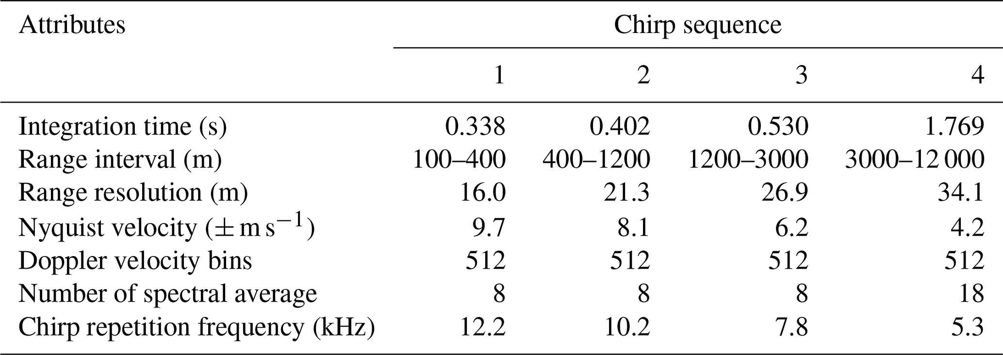
JOYRAD-94, hereafter referred to as the W band, is a 94 GHz frequency-modulated continuous-wave (FMCW) radar, combined with a radiometric channel at 89 GHz. The instrument is manufactured by Radiometer Physics GmbH (RPG), Germany. Unlike the X and Ka band radar, the W band radar is a non-polarimetric, non-scanning, and non-pulsed system. The W band started measurements at JOYCE-CF in October 2015; a detailed description of the radar performance, hardware, signal processing, and calibration can be found in Küchler et al. (2017). The W band radar has a similar beam width, range, and temporal resolution as the Ka band (Table 1). The FMCW system allows the user to set different range resolutions for different altitudes by acting on the frequency modulation settings (chirp sequence). During TRIPEx the standard chirp sequence (Table 2) was used. After correcting the Doppler spectra for aliasing using the method described in Küchler et al. (2017), standard radar moments such as the equivalent Ze, MDV, and SW are derived.
Table 1Technical specifications and settings of the three vertically pointing radars operated during TRIPEx at JOYCE-CF.

Table 2Main settings of the chirp sequence used during TRIPEx for the W band radar. See Küchler et al. (2017) for a detailed description.
The full TRIPEx dataset is structured on three processing levels. Level 0 contains the original data from the X, Ka, and W band. For Level 1, the measurements are corrected for known instrument problems and sampled into a common time–height grid. At this stage, the data can still be considered raw; further processing steps that are either dependent on radar frequency or atmospheric conditions are applied to the Level 2 dataset. These processing steps include the detection and removal of measurements affected by ground clutter, an offset correction of the radars based on independent sources, the compensation for estimated differential attenuation caused by atmospheric gases, adjustment of the DWRs by cross calibrations between the three radars and the addition of data quality flags. These steps are meant to remove spurious multifrequency signals that are not produced by cloud properties. The processing is performed to the best of our knowledge; however, intermediate steps are included in the dataset in order to allow the original data to be recovered at any stage and different processing techniques to be applied. Figure 2 illustrates the work chain from Level 0 to Level 2. The following sections provide a detailed description of each step.
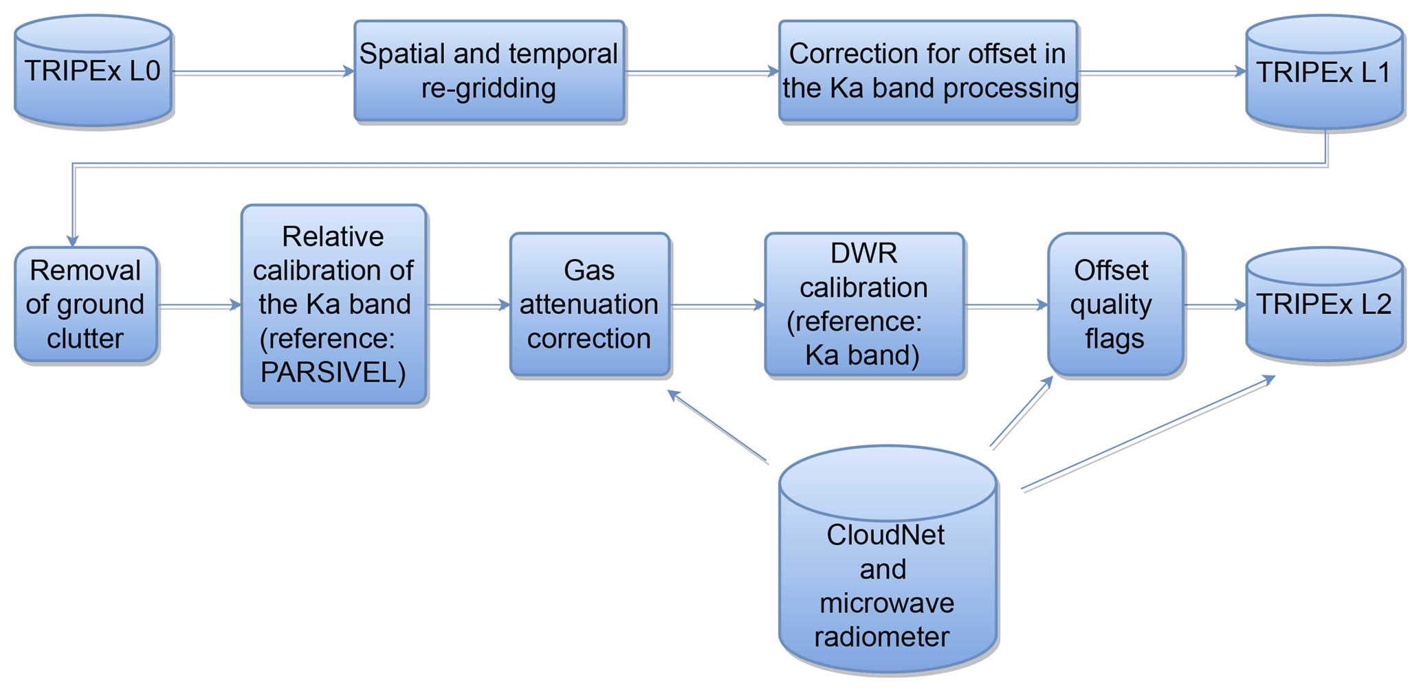
Figure 2Flowchart of the TRIPEx data processing. The upper part describes the steps producing data Level 1 and the bottom part those producing data Level 2.
3.1 Spatiotemporal re-gridding and offset correction
Since the range and temporal resolutions of the three radars are slightly different (Table 1), the data are re-gridded at a common time and space resolution in order to allow for the calculation of dual wavelength ratios (DWRs) defined for two wavelengths λ1 and λ2 as
with Zeλ in dBZ. The reference grid has a temporal resolution of of 4 s and a vertical resolution of 30 m, which is the resolution of the W band. The data are interpolated using a nearest-neighbor approach, with the maximum data displacement limited to ±17 m in range and ±2 s in time. This method preserves the high-resolution information of the original radar observations. Limiting the interpolation displacement avoids spurious multifrequency features that may result from nonmatching radar volumes. Residual volume mismatches may occur at cloud boundaries where heterogeneities are largest. For the Ka band, two corrections are applied to the original reflectivity as suggested by the manufacturer (Matthias Bauer-Pfundstein, Metek GmbH, personal communication, 2015). An offset of 2 dB is added to account for power loss caused by the finite receiver bandwidth; another 3 dB offset is added to correct for problems in the digital signal processor used in older MIRA systems. These corrections are applied for processing of the Level 1 data.
3.2 Clutter removal
Following the corrections for radar offsets and re-gridding, the first step in the Level 2 processing is the removal of the range gates affected by ground clutter. Considering the different radar installation locations (roof mount or ground surface) and antenna patterns, the clutter contamination affects each type of radar data differently. The thresholds for the lowest usable range gates are determined empirically and are reported in Table 1.
3.3 Evaluation of the Ka band calibration with PARSIVEL disdrometer measurements
The three radars have been individually calibrated by their respective manufacturers; however, radar components might experience drifts over time, which can lead to biases of several dB. The JOYCE site is equipped with a PARSIVEL optical disdrometer (Löffler-Mang and Joss, 2000), which provides the drop size distribution (DSD) with a temporal resolution of 1 min. For rainfall events, the DSD can be used to calculate the associated radar reflectivity factor. In this study, the scattering properties of raindrops are calculated using the T-matrix approach (Leinonen, 2014) with a drop shape model that follows Thurai et al. (2007) and assuming drop canting angles that follow a Gaussian distribution with zero mean and 7∘ standard deviation (Huang et al., 2008). Unfortunately, the lowest usable radar range gates are 500–600 m above the PARSIVEL; thus we have to assume a constant DSD over this altitude range in order to compare with the radar reflectivities. Time lags and wind shear effects raise further problems in the direct comparisons between radar-measured Ze and the one calculated with PARSIVEL. For this reason, we only compare the statistical distribution of reflectivities at the lowest range gates measured over several hours with the corresponding distribution calculated at the ground level. Of course, systematic differences caused by rain evaporation, drop breakup, or drop growth due to accretion towards the ground may affect such comparisons. However, the changes in the Ze profile are very close to the ones predicted by attenuation and constant DSD from three light rainfall cases. The reflectivity distributions from PARSIVEL and the Ka band (Fig. 3) of those periods are very similar but differ by approximately 3.6 dB, with the Ka band having the lower reflectivities. For these comparisons, periods before and after the TRIPEx campaign had to be used because PARSIVEL had a hardware failure during the campaign. The similarity of the results gives us an indication that this method is reliable; however, a large number of cases are still needed in other to draw a final conclusion on this method. Unfortunately, only the Ka band was available because the other two radars did not measure during the selected rainfall events.
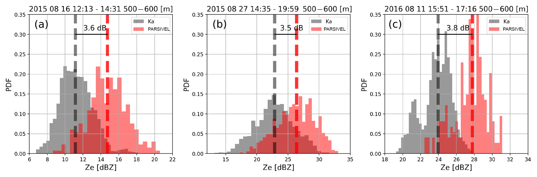
Figure 3Histograms of radar reflectivities from the Ka band (gray) and results from T-matrix calculations with the raindrop size distribution provided by PARSIVEL (red) for three long-lasting stratiform rain cases before and after the TRIPEx campaign (a 16 August 2015, b 27 August 2015, c 11 August 2016). Ka band reflectivities are taken from the lowest clutter-free range gates between 500 and 600 m. The vertical dashed line indicates the median of the distribution; the offset is calculated as the difference between Ka band and T-matrix results.
3.4 Correction for atmospheric gas attenuation
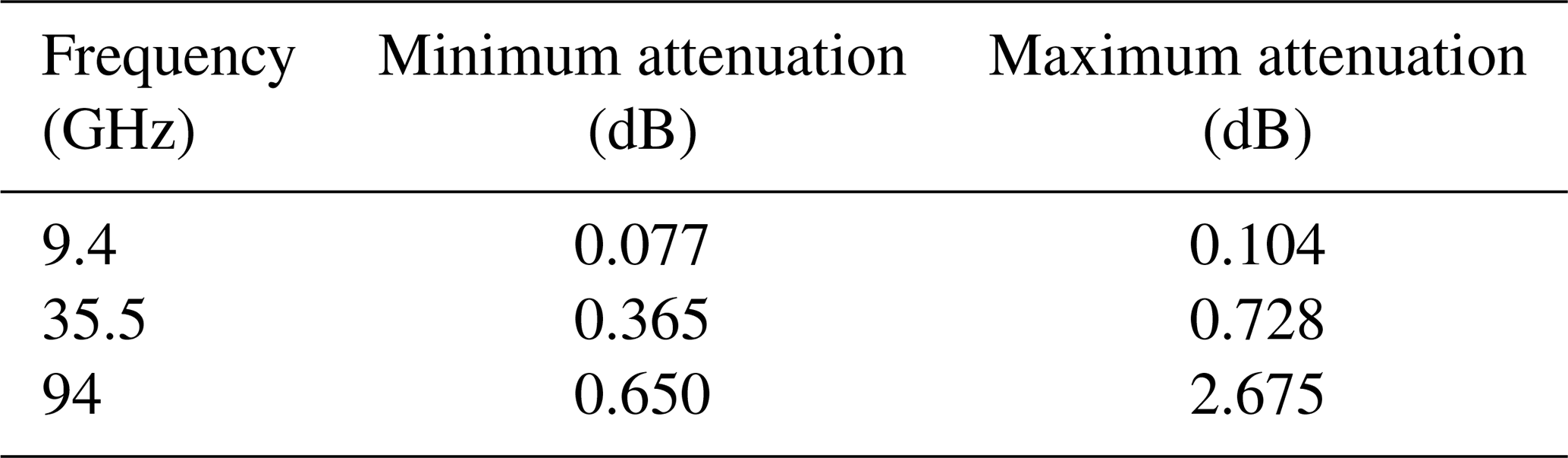
Hydrometeors and atmospheric gases cause considerable attenuation at cloud radar frequencies. The reflectivities from the X, Ka, and W band are corrected for estimated attenuation due to atmospheric gases (Fig. 2) by means of the Passive and Active Microwave TRAnsfer model (PAMTRA) (Maahn et al., 2015). PAMTRA calculates specific attenuation due to molecular nitrogen, oxygen, and water vapor based on the gas absorption model from Rosenkranz (1993, 1998, 1999). Input parameters are the vertical profiles of atmospheric temperature, pressure, and humidity provided by the CloudNet products (Illingworth et al., 2007), which are generated operationally at the JOYCE-CF site. The two-way path-integrated attenuation (PIA) at the radar range gates is derived from the specific attenuation integrated along the vertical. Table 3 lists the minimum and maximum two-way attenuation values at ≈12 km (height of the maximum range gate in Level 2 data) for the three radars during the entire campaign. The highest attenuation of ≈2.6 dB occurs at 94 GHz and is mainly caused by water vapor. Conversely, the 9.4 GHz maximum attenuation of ≈0.1 dB is the lowest among the three radars, and it is mainly produced by oxygen continuum absorption. At 35.5 GHz, attenuation is governed by both oxygen and water vapor. The maximum attenuation value found at this frequency is ≈0.7 dB.
Table 3Calculated minimum and maximum two-way path-integrated attenuation (PIA) at a height of ≈12 km for the X, Ka, and W band during TRIPEx.
3.5 DWR calibration and generation of quality flags
Spurious multifrequency signals can arise from attenuation effects due to particulate atmospheric components (e.g., liquid water, melting layer, and snow) but also from instrument-specific effects such as a wet radome, snow on the antenna, and remaining relative offsets due to radar miscalibration. With this processing step, the reflectivity measurements are adjusted in order to take into account the cumulative effects of the aforementioned bias mechanisms at the top of the clouds. By doing so, the effects of the cloud microphysical processes on the DWR signals are recovered.
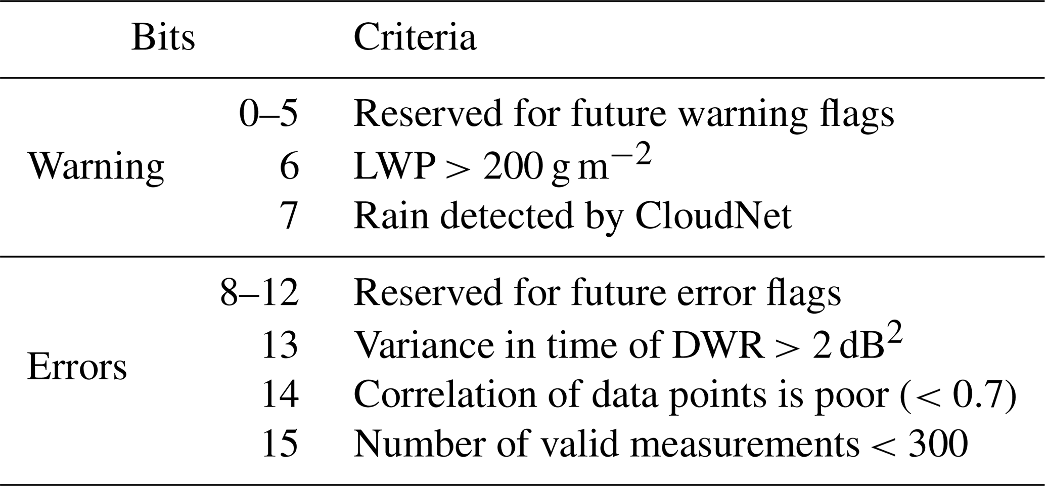
The Ka band is used as a reference because of its better sensitivity level and larger dynamic range compared to the other radars (up to high altitudes) and its lower signal attenuation compared to the W band. Moreover, the Ka band is the only system not equipped with a radome which might collect raindrops on its surface and cause additional attenuation. The signal attenuation due to antenna wetness on the Ka band is expected to be lower compared to other radars' radome attenuation because of the periodic antenna tilts during RHI scans (every 30 min). The processing is complemented by the generation of quality flags categorized as errors and warnings. Error flags mark data of poor quality based on the applied correction procedure, while warnings indicate the detection of potential sources of DWR offsets that have not been accounted for in the procedures described below. An additional error flag is raised if spurious multifrequency signals due to radar volume mismatch are suspected. A list of all the quality flags (both errors and warnings) is provided in Table 4.
The small ice particles in the upper parts of clouds are mostly Rayleigh scatterers (Kneifel et al., 2015; Hogan et al., 2000); thus, their reflectivities should not be frequency-dependent (Matrosov, 1993). The reflectivity range, at which the Rayleigh approximation can be assumed, is estimated by investigating the behavior of the observed DWRs as a function of ZeKa. Within the Rayleigh regime, the measured DWRs are expected to remain constant at a value that accounts for all the integrated differential attenuation and radar miscalibration effects. As the ice particles grow larger, the DWRs start to deviate from that constant value, and this deviation affects the higher-frequency radars first. Because of that, the Rayleigh data have been isolated by means of two different reflectivity thresholds for X and W band radars. In addition, the sensitivity of the X band is much lower; thus, a higher reflectivity threshold is accepted for the offset estimate between the X and Ka band compared to the Ka and W band. For the determination of the relative offset for the W band, we found an optimal range of dBZ and dBZ for the X band. In order to safely exclude partially melted particles, only reflectivities from at least 1 km above the 0 ∘C isotherm are used.
The relative offset correction is estimated for each measuring time from the data inside a moving time window of 15 min. The selected data are restricted to the reflectivity pairs, which are within threshold values defined above. The mean value of the DWR computed for these reflectivity pairs constitutes the DWR offset. The quality of this offset estimation strongly depends on the quality and quantity of the reflectivity data included in the average. Empirical analysis showed that at least 300 data points spanning a wide reflectivity range are required in order to have acceptable sampling errors. The data that present smaller sampling statistics are marked with an error flag.
Whenever cloud edges are included in the sampling volume, and/or when the measured Ze is close to the sensitivity limits of the instruments, the correlation between the reflectivities of two radars might strongly deteriorate. In order to help the user identify these potential sources of errors, the data profiles presenting a correlation lower than 0.7 are marked with an additional error flag.
Despite the matching procedure of the different frequency radar volumes (Sect. 3.1), mismatches are unavoidable due to the horizontal distances between the radars (Fig. 1) and the different radar range resolutions and beam widths (Table 1). At cloud edges and close to the melting layer, where the largest spatial cloud inhomogeneities are expected, the effects of the remaining radar volume mismatches will be maximized. The temporal DWR variability during 2 min moving windows is used as an indicator for a potential volume mismatch; cloud regions with variances above 2 dB2 are flagged accordingly.
Table 4Quality flags included in the data Level 2 product (bit coded in a 16-bit integer value). The flags indicate the reliability of the data and in relation to the quality of the relative offset estimate for X-Ka and W–Ka band reflectivities. Note that offsets are not calculated when the number of reflectivity pairs is below 300.
The described adjustment technique accounts for all processes that affect relative offsets of the radars in the upper and frozen part of clouds. These processes include possible frequency-dependent attenuation effects from lower levels, radar miscalibration, and radome and antenna attenuation. Since the estimated correction is applied to the entire profile, inevitably overcompensations might occur in the lower, possibly rainy parts of clouds. This limitation is necessary in order to increase the quality of the data in the ice part of the clouds, which is the main focus area of the presented study.
The lack of information about vertical hydrometeor distribution prevents reliable reflectivity corrections by differential attenuation. As a consequence of the presented DWR calibration and the fact that hydrometeor attenuation is hitting the higher frequencies more, the computed DWRs are expected to be increasingly underestimated towards the ground. A refined correction should be applied for rain and melting layer studies. Possible sources of information about the amount and position of supercooled liquid water could be collocated lidar or analysis of radar Doppler spectra measurements. Those data are available at JOYCE-CF, but they are not included in the current dataset. However, an additional warning flag indicates periods with large liquid water paths derived from the collocated microwave radiometer. Lastly, the occurrence of rainfall and/or a melting layer from the CloudNet classification and indicated by the precipitation gauge is marked with an additional warning flag (Table 4).
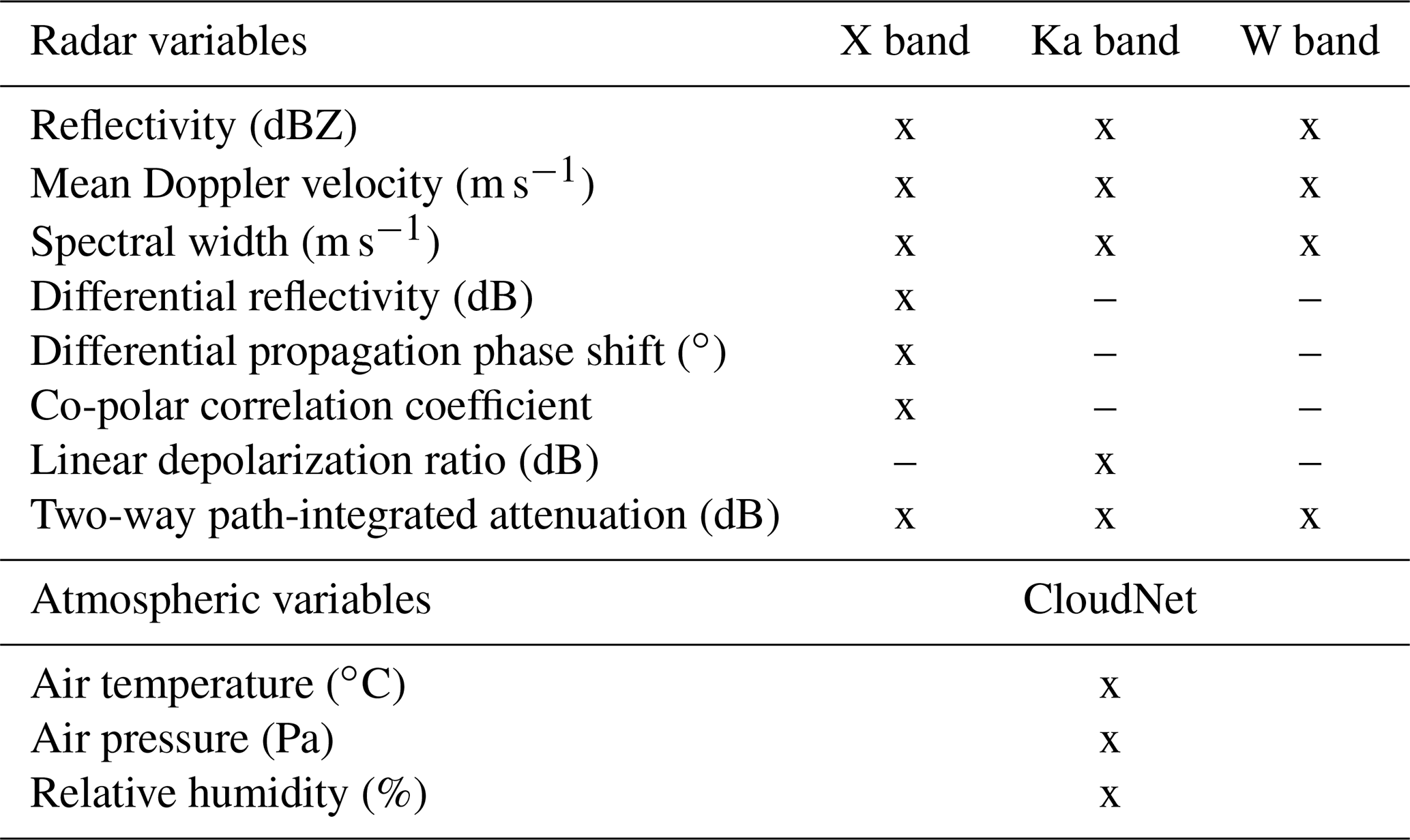
The Level 2 of the TRIPEx dataset contains radar moments, polarimetric variables, integrated attenuation, and atmospheric state variables. The polarimetric variables are included as they are provided by the radar software, and no additional processing or quality check is applied to them. Zdr, ϕdp, and ρhv from the X band might be a useful additional source of information for melting layer studies (Zrnić et al., 1994; Baldini and Gorgucci, 2006). We are not confident about the quality of Kdp provided by the X band software, and therefore, this variable is not included in the dataset but can be calculated by the user. Table 5 lists all variables available in Level 2.
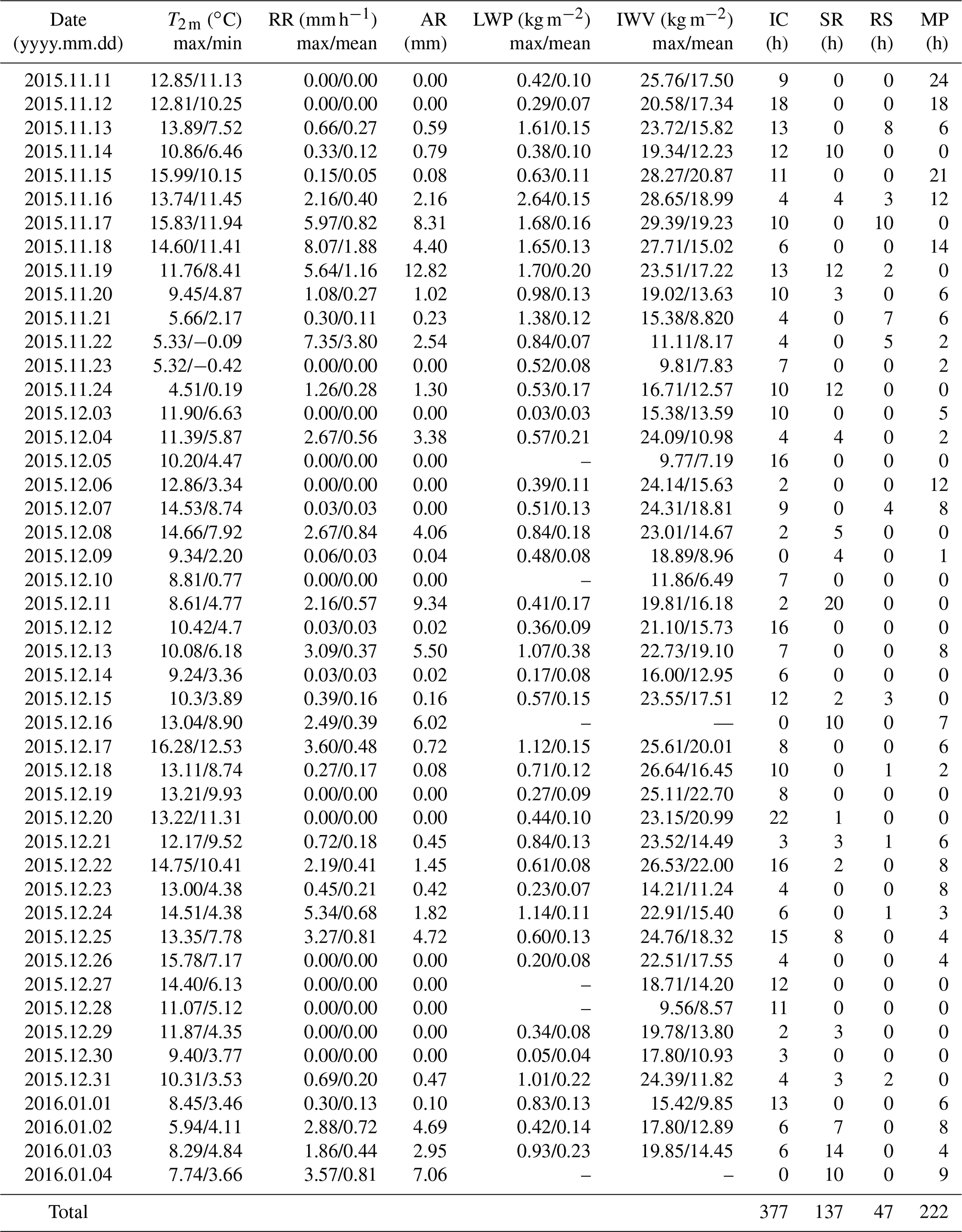
The dataset contains 47 days of measurements. For each day, Table 6 lists the atmospheric conditions such as temperature at 2 m (T2 m), rain rate (RR), accumulated rain (AR), liquid water path (LWP), and integrated water vapor (IWV). The duration of four empirically classified predominant types of cloud and precipitation is provided for each day (Table 6). The two most frequent cloud types are ice clouds (IC) with 377 h and shallow mixed-phase clouds with 222 h of observations. Stratiform rainfall (SR) occurred during 137 h, while rain showers (SR) were only observed during 47 h. The average rain rate (RR) for all rainy periods over the whole period (mean rain intensity) is 0.078 mm h−1, with a maximum instantaneous RR of 8.07 mm h−1. DWR signatures and radar Doppler information suggest that the ice part of clouds is dominated by depositional growth and aggregation. Riming only seems to occur during a few short events. Although the dataset spans the main winter season, no snowfall was recorded at the surface. In the following, we will demonstrate the effect of applying data quality flags and discuss remaining limitations as well as the effects of the different radar sensitivities.
Table 6Characterization of the atmospheric conditions and estimated duration of cloud and precipitation events during TRIPEx. T2 m is the air temperature at 2 m from a nearby weather station. RR and AR are the rain rate and the accumulated rain measured by a Pluvio disdrometer; mean RR is calculated using all RR values larger than 0 mm h−1. Liquid water path (LWP) and integrated water vapor (IWV) are derived from the collocated 14-channel microwave radiometer; mean LWP is calculated using all LWP values larger than 0.03 kg m−1 in order to exclude clear-sky periods. The columns with IC, SR, RS, and MP indicate the approximate duration in hours of non-precipitating ice clouds, stratiform rain, rain showers, and shallow mixed-phase clouds, respectively.
4.1 Effects of data filtering based on quality flags
The effects of data filtering on DWRXKa and DWRKaW are demonstrated for clouds observed on 20 November 2015 in Figs. 4 and 5. In order to give a better visual impression of these effects, the filtering steps are applied sequentially and cumulatively. Figure 4a–c show the unfiltered Level 2 data. The time–height plots (Fig. 4a and b) reveal a stratiform cloud passing over the site from 01:00 to 17:00 UTC, followed by a series of low-level, shallow, most likely mixed-phase clouds. The short periodic gaps result from interruptions of zenith observations caused by range-height indicator (RHI) scans of the Ka band, and the large gap in DWRKaW between 09:00 and 10:00 UTC is caused from missing W band observations. The −15 ∘C isotherm (dashed line in the time–height plots) separates DWRs around 0 dB for temperatures below −15 ∘C from rapid increases with reflectivity for higher temperatures.
Figure 4c displays a scatter density plot of DWRXKa versus DWRKaW (hereafter called the triple-frequency plot). The position in the triple-frequency plot is mainly driven by the respective hydrometeors' bulk density ρ and their mean volume diameter D0 (Kneifel et al., 2015). This plot allows discrimination between the two processes: rimed particles follow the flat curve (low DWRXKa) due to their higher density, while aggregated particles give rise to a bending-up signature (increase in DWRXKa, while DWRKaW saturates or even decreases) due to their lower density, which is nicely shown in Fig. 4c.

Figure 4Time–height plots of DWRKaW (a) and DWRXKa (b) using the Level 2 data of 20 November 2015 without applying any filtering. The continuous line and dashed line are the 0 and −15 ∘C isotherms (provided by the CloudNet products), respectively. The triple-frequency signatures for the ice part of the clouds are shown in (c). Panels (d–f) show the remaining data after applying the offset quality flags and the restriction to data pairs with sufficient correlation. N in (c, f) indicates the respective number of data pairs in the ice part of the clouds. Note the log scale on the color bars in (c, f).
A large number of points in Fig. 4c populate areas which are unrealistic from a microphysical point, such as negative DWRs. Some of those originate from time periods when the offset cannot be calculated properly or when the correlation between the three radars is poor. Figure 4d and e show the results after removing those points (bits 14 and 15 in the quality flag; see Table 4), an effect best visible between 17:00 and 20:00 for DWRKaW and between 17:00 and 23:00 for DWRXKa. The triple-frequency plot (Fig. 4f) shows a strong reduction of outliers when compared to the unfiltered triple-frequency plot (Fig. 4c).
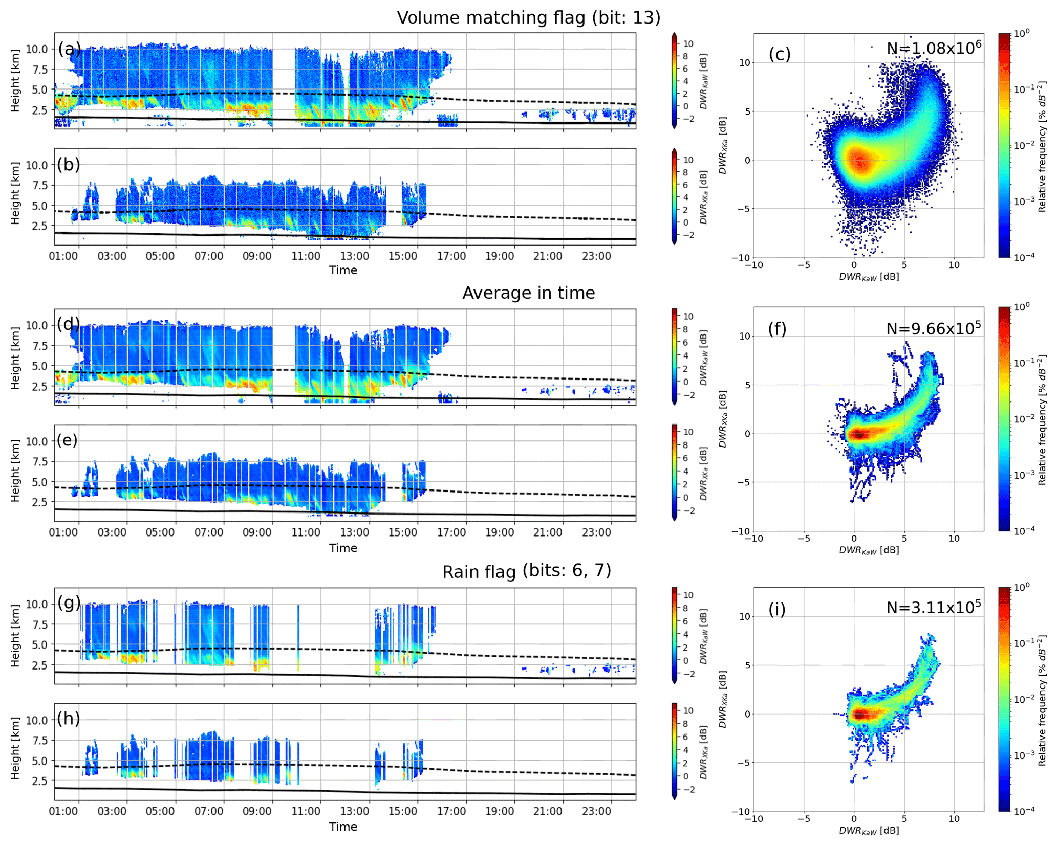
Figure 5Same as Fig. 4, but here the effects of cumulative data filtering subject to different quality flags and averaging are illustrated. Panels (a–c) display the effect of filtering based on the DWR variance in time, which removes areas potentially affected by poor radar volume matching. The effect of the additional temporal averaging over 3 min is shown in (d–f). The effects of the removal of time periods with rain as identified by CloudNet or large liquid water paths measured by the nearby microwave radiometer are displayed in (g–i). Note the log scale on the color bars in (c, f, i).
Despite the data filtering described in the previous paragraph, the scatter around the main signature is still large. Figure 5a and b show the time–height plots after removing observations flagged with the DWR 2 min temporal variance flag (bit 13 in the quality flag; see Table 4). This filtering step removes most of the outliers from the aggregation signature in the triple-frequency plot (Fig. 5c). It is worth noting that the removal of such data reduces the scatter in the triple-frequency space but might also remove interesting measurements from regions with strong reflectivity gradients. Additional 3 min running-window averaging of the reflectivities keeps the most stable signatures (Fig. 5d and e), further removes scatter, and thus accentuates the aggregation signature in triple-frequency plot (Fig. 5f). The averaged reflectivities calculated in this procedure are not included in the TRIPEx dataset because it would not be possible to retrieve the original data. The last two quality flags (bits 7 and 6; see Table 4) mark data acquired during rainfall according to the CloudNet product and times with total liquid water path larger than 200 g m−2 as estimated by the microwave radiometer. The latter filtering significantly reduces the amount of usable data (Fig. 5g and h) but preserves the main aggregation signature surprisingly well (Fig. 5i).
4.2 Limitations of the current dataset
Despite the filtering steps discussed in Sect. 3.5, some limitations remain. As an example, on 23 November 2015 between 16:00 and 23:00 UTC we observe enhanced values of ZeX (−20 up to 10 dBZ) (Fig. 6a), while ZeKa and ZeW remain very low. The mean Doppler velocity of that structure is very small (MDV between 0 and 0.5 m s−1) and is associated with a strongly enhanced LDR from the Ka band (Fig. 6b). Large Zdr values are observed by the nearby weather polarimetric X band radars JuXPol and BoXPol (see Diederich et al., 2015, for a detailed characterization of the radars) that were performing RHI scans over the TRIPEx site at that time. The most likely explanation based on the polarimetric signature and the fall velocity is fall streaks of chaff deployed by military aircraft during a training session. We recommend avoiding this period in cloud microphysical studies.
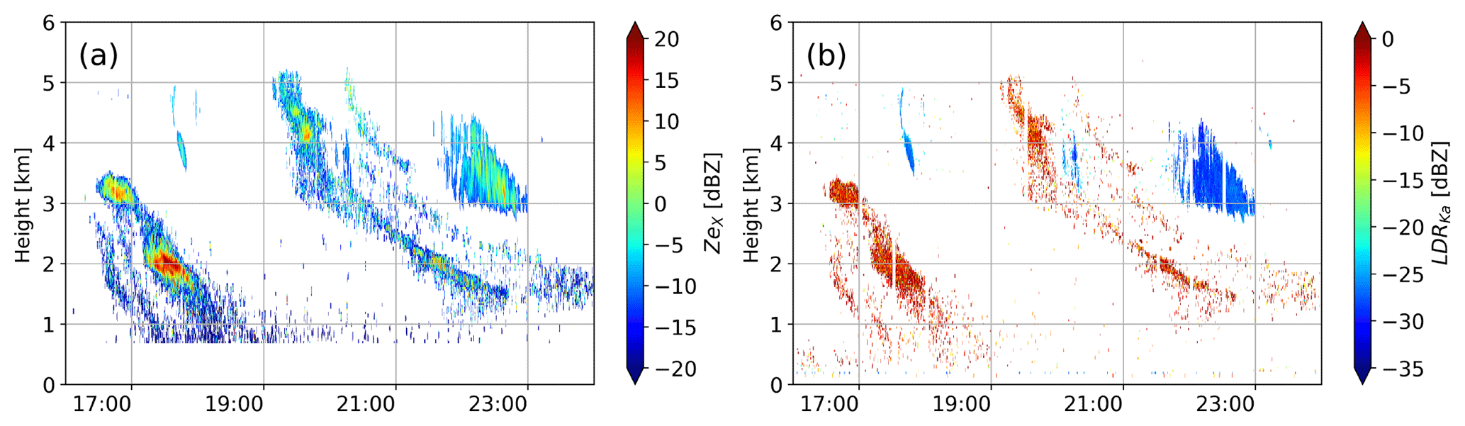
Figure 6Time–height plots of the ZeX and LDRKa of 23 November 2015 between 16:00 and 23:59. The region where the LDR is dB is most probably the result of chaff. The Ka band software applies a filtering for non-meteorological targets which removes most of the chaff; only the filtered Ka band data are included in the TRIPEx dataset. Note that no such filtering is applied to the X band and W band data.

Figure 7Time–height plots of the dual mean Doppler velocity using the Level 2 data of 20 November 2015. The dashed line and the continuous line are the −15 and 0 ∘C isotherms, respectively. Panel (a) shows the DDVXKa using the original data from Level 2. Panel (b) shows the DDVXKa after applying a 3 min moving average.
As described in Sect. 2.1, the X band was operated vertically pointing while rotating the antenna. Figure 7 illustrates effects related to imperfect vertical antenna pointing. When looking at the differences between vertical Doppler velocities observed from low-frequency and high-frequency radars (dual Doppler velocity, DDV), increases are expected in the presence of large scatterers (Matrosov, 2011; Kneifel et al., 2016). Large particles, which usually also have greater terminal velocities, give a lower reflectivity signal at high frequencies due to non-Rayleigh scattering. This effect also leads to a lower MDV (MDV). Since the ice particles in the uppermost part of the clouds are expected to be Rayleigh scatterers, the DDV should be zero. However, DDVXKa (Fig. 7a) shows a periodic variation along the entire vertical range, with the period matching the X band scan duration of 3 min. Obviously, a non-perfect zenith pointing of the X band antenna introduces these periodic shifts in the mean Doppler velocity due to the contamination of the vertical Doppler signal by the horizontal wind component. A temporal average over 3 min minimizes the standard deviation of DDVXKa relative to other averaging window sizes (Fig. 7b). Note that the averaged data are not included in the Level 2 data product because the optimal averaging window might depend on the prevailing atmospheric, height-dependent wind conditions, and original data cannot be recovered after averaging. We can also not completely rule out a slight mispointing of the other two radars because their DDVs sometimes show deviations, especially in regions with strong horizontal winds with maximum DDVs. However, these DDVs are found to be below 0.4 m s−1. An ad hoc estimate of the related relative radar mispointing of the two radars using the horizontal wind information from radiosondes for a few extreme cases suggests a potential mismatching of 0.5∘. A correction of the shift requires reliable horizontal wind profiles, which will be investigated in more detail in the future.
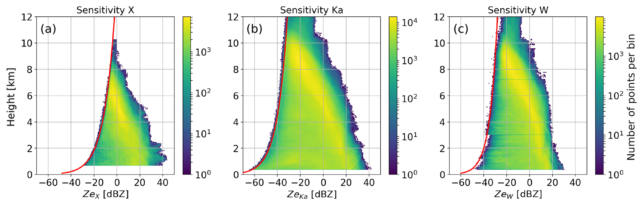
Figure 8Histograms of reflectivities from the entire TRIPEx campaign Level 2 data for each radar. The red curve is the profile of the minimum retrieved reflectivity (Eq. 2). Panels (a), (b), and (c) show the histograms for the X, Ka, and W band, respectively; all error flags (see Table 4) were applied to filter the data. Note the log scale on the color bars.
4.3 Radar sensitivity
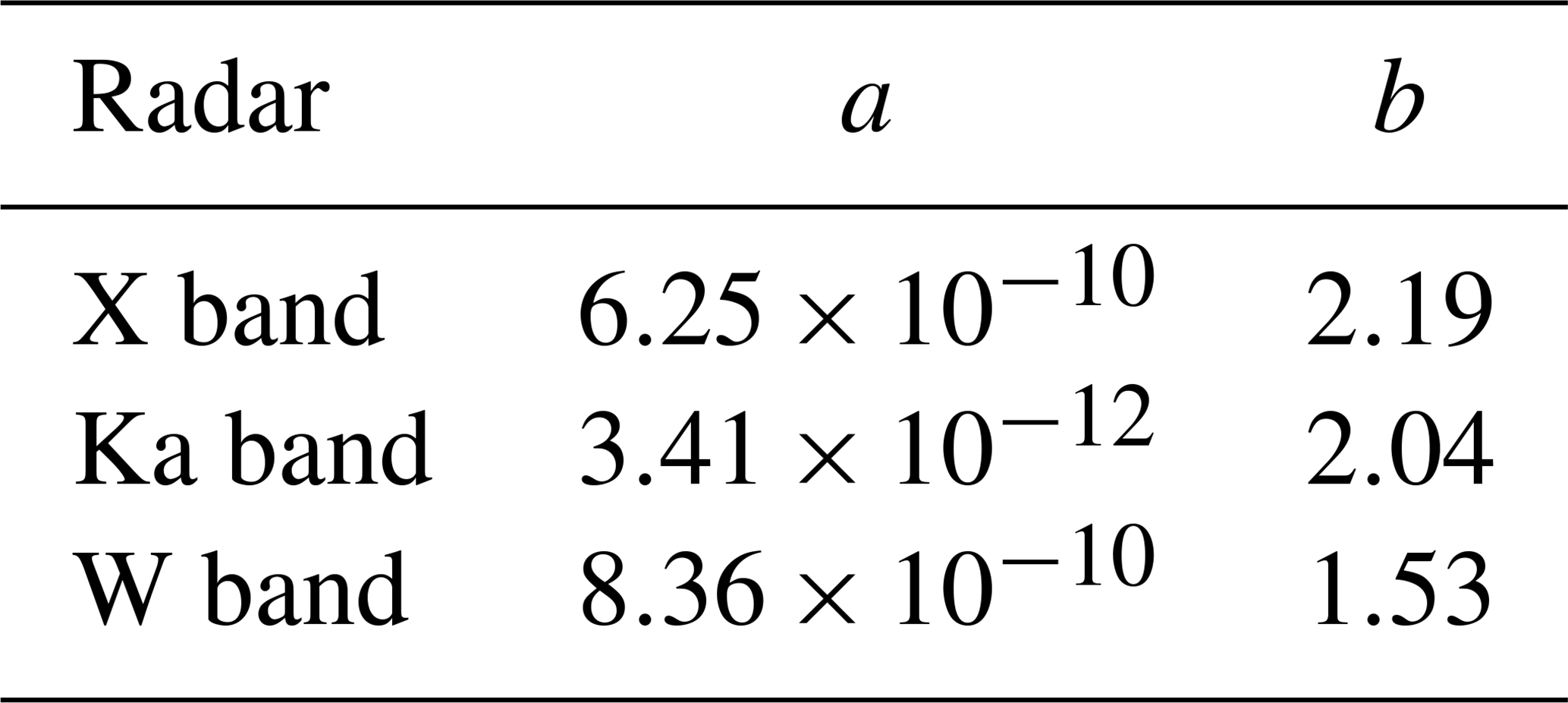
Figure 8 shows the distribution of reflectivity values measured by the three radars during the entire campaign filtered with the error flags (bits 13, 14, and 15 in Table 4) and stratified by height above the site. As already mentioned, the Ka band and W band show higher sensitivities compared to the X band up to high altitudes. The Ka band (Fig. 8b) exhibits the largest dynamic range (Fig. 8a and c). The step-like shape of the lowest altitude reflectivities from the W band is caused by different chirp settings (Table 2). A polynomial fit to the minimum retrieved linear reflectivities (Zelin, in units of mm6 m−3) as a function of altitude z (units of m),
results for the X and Ka band in the expected nearly quadratic decrease with range (Table 7). The slower decrease (smaller exponent) for the W band results from the altitude-dependent sensitivity associated with the height-varying chirp settings.
The melting layer was mostly observed at altitudes between 1 and 2 km, where it causes a sharper increase in the reflectivity distribution and the largest values measured for the X band reflectivities. The X band Ze distribution shows an enhancement of the largest recorded values at 2 km from ≈30 to ≈40 dBZ. The X band sensitivity limitations did not allow signals above 7 km with reflectivities below −10 dBZ to be observed; however, dual-wavelength studies of clouds in this region are still possible with the W band and Ka band included in the Level 2 data. Nonetheless, ice aggregation and riming, which are most relevant for triple-frequency studies, usually occur at lower levels and larger reflectivities where all three radars provide sufficient sensitivity.
Longer time series of observations are required in order to reliably estimate the occurrence probabilities of process signatures in the triple-frequency space. Those statistics might be useful for the development of microphysical retrievals and to constrain snow particle scattering models. Currently available datasets are restricted to short time periods or specific cases. Kulie et al. (2014) and Leinonen et al. (2012) used observations from airborne Ku, Ka, and W band radars data collected during the Wakasa Bay campaign (Lobl et al., 2007) to evaluate aggregate and spheroidal snowflake models. Their DWRKaW and DWRKuKa values reach up to 10 and 8 dB, respectively. Although their data are rather noisy due to volume mismatch and attenuation effects, they were the first observations which confirmed triple-frequency signatures predicted by complex aggregate scattering models (Kneifel et al., 2011a). The first triple-frequency signatures from ground-based radars (S, Ka, and W band) were presented by Stein et al. (2015) for two case studies. Similar to the Wakasa Bay studies, they found deviation from predictions based on simpler spheroidal-based scattering models, but their aggregates showed a DWRKaW saturation around 8 dB and not the “hook” or “bending back” feature found in the previous studies. They attributed this behavior to a snow aggregate fractal dimension of 2. Kneifel et al. (2015) combined triple-frequency ground-based radar (X, Ka and W band) with in situ observations and analyzed three cases characterized by falling snow particles with different degrees of riming. For low-density aggregates, their DWRKaW also did not exceed the 8 dB limit reported by previous studies but exhibited a strong bending back feature (i.e., reduction of DWRKaW for larger particles) with large DWRXKa up to 15 dB. During riming periods, the triple-frequency signatures showed a distinctly different behavior: DWRKaW increases up to 10 dB, while DWRXKa remains constant or slowly increases up to 3 dB, which appears in triple-frequency plots as an almost horizontal line.

Figure 9Two-dimensional histograms (contoured frequency by altitude diagram, CFAD; see Yuter and Houze, 1995, for more details) of DWR against air temperature for the entire TRIPEx dataset. The dashed line indicates the 0 ∘C isotherm. The data below the dashed line are only collected from the cases in which a melting layer is observed. The DWRs were filtered using the error flags and averaged in time using a 3 min moving window. Panels (a) and (b) show DWRKaW and DWRXKa, respectively. Note the log scale of the color bars.
The TRIPEx dataset is, to the best of our knowledge, one of the longest, quality-controlled triple-frequency datasets currently available, which allows for reliable estimations of the occurrence of several triple-frequency signatures in midlatitude winter clouds. In the following sections, we use the Level 2 data filtered only with the error quality flag (see Table 4) to analyze the temperature dependence of the triple-frequency signatures and signatures of riming and melting snow particles. The extension of the filtering to the warning flags would remove all melting layer cases and/or observations with larger amounts of supercooled liquid water, which portray particularly interesting signatures of partially melted or rimed particles.
5.1 Temperature dependence of triple-frequency signatures
The relatively large dataset allows us to stratify the occurrence probability of DWRKaW (Fig. 9a) and DWRXKa (Fig. 9b) according to air temperature, which results in four main regimes. The regime in which the temperature is smaller than −20 ∘C exhibits small DWR values, mostly below 3 dB.
Between −20 and −10 ∘C, we find a widening of the distribution to higher values in both DWRs. This DWR increase becomes very rapid at temperatures warmer than −15 ∘C, which suggests an increasing number of larger aggregates caused by stronger aggregation due to preferential growth of dendritic particles in the −20 to −10 ∘C temperature range (Kobayashi, 1957; Pruppacher and Klett, 1997). Dendrites are well known to favor snow aggregation due to their branched crystal structure. In accordance with previous studies, DWRKaW saturates around 7 dB at −10∘C, with only a small fraction reaching up to 10 dB. DWRXKa approaches maximum values of 5 to 8 dB; however, the occurrence probability of enhanced DWRXKa is smaller compared to those found for DWRKaW. This is an expected behavior since early aggregation is likely to first enhance the DWRKaW because particle growth affects the high frequencies early which first transition out of the Rayleigh regime. Thus the W band radar is the first influenced by this transition which enhances DWRKaW.
At temperatures between −10 and 0 ∘C, the distribution of DWRKaW remains almost constant, with the exception of a small peak with higher values around −5 ∘C and a widening of the DWR distributions towards negative values. The latter effect might relate to two causes. The first is the DWR calibration (Sect. 3.5), derived for the upper part of the clouds (ice part), which, when applied to the entire profile, leads to the overestimation of ZeW. The second possible contributor is the radar volume mismatch, which becomes worse for observations closer to the radars due to reduced overlap of the radar beams.
Interestingly, DWRXKa grows continuously up to 12 dB for temperatures warmer than −5 ∘C, which is in line with intensified aggregation of the snow particles towards lower heights. The very large DWRXKa in this regime can be explained by increasing particle stickiness when approaching the 0 ∘C level. In the fourth regime between 0 ∘C and the LDR maximum, DWRKaW tends to further increase, while DWRXKa remains constant or even decreases. DWRKaW reaches values up to 10 dB, while DWRXKa attains values up to 15 dB, which could be produced by persistent aggregation.
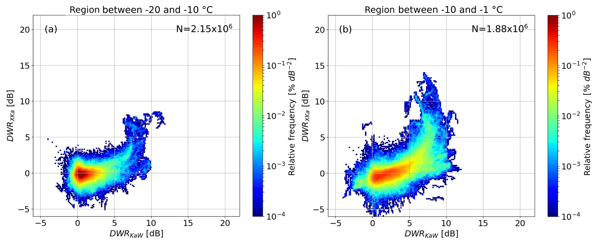
Figure 10Two-dimensional histogram of the triple-frequency signatures for different temperature regions normalized by the total number of points N. The color shows the relative frequency. Panel (a) is for temperatures between −20 and −10 ∘C. Panel (b) shows the region between −10 and −1 ∘C. Note the log scale on the color bars.
Figure 10 shows the triple-frequency plots for the temperature ranges ∘C (panel a) and ∘C (panel b). Between −20 and −10 ∘C (panel a), we find the typical bending signature in the triple-frequency space saturating at about a DWRKaW of 8 dB, similar to Stein et al. (2015). This temperature regime includes the dendritic growth zone (DGZ), which is usually defined by cloud chamber experiments in the range of temperatures −17 to −12 ∘C (Kobayashi, 1957; Yamashtta et al., 1985; Takahashi, 2014). It is worth reminding the reader that the temperature information included in the TRIPEx dataset has not been obtained from a direct measurement, but it has been taken from CloudNet. Consequently, it is not surprising that the growth regimes that we have identified using the signatures observed in the DWR profiles do not perfectly correspond in temperature to the ones determined in cloud chamber experiments.
Although we combine observations from different clouds, the variability of the triple-frequency signatures is relatively small. For warmer temperatures (−10 to −1 ∘C, panel b), needle aggregates are likely to be generated, and ice particles start to become more sticky, leading to a more pronounced bending feature. For DWRXKa reaching up to 12 dB, the hook (or bending back) signature (Kneifel et al., 2015) also becomes visible for parts of the dataset (DWRXKa decreases, while DWRKaW is still increasing). This panel also reveals a secondary mode with DWRXKa below 3 dB and DWRKaW reaching up to 12 dB. Following Kneifel et al. (2015), this mode could hint at rimed particles, which are still too small to enhance DWRXKa, but due to their increased density and hence larger refractive index, the DWRKaW increases. We will investigate this feature in more detail in the next subsection.
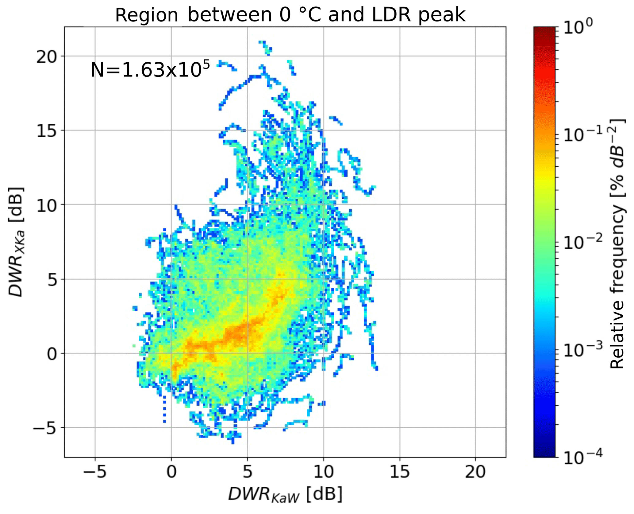
Figure 11Two-dimensional histogram of the triple-frequency signatures for the region between 0 ∘C and the LDR maximum in the melting layer normalized by the total number of points N. The color shows the relative frequency, and the binning matches what was used for Fig. 10. Note the log scale on the color bar.

Figure 12Triple-frequency signatures for Level 2 data with temperatures between −20 and −1 ∘C and a mean Doppler velocity (MDV) above 1.5 m s−1 in order to select potentially rimed particles. Panel (a) shows the relative frequency of the observations. Panel (b) indicates the average MDV of each pixel in the histogram. Note the log scale on the color bar in (a).
The dataset contains particularly large DWR signatures close to 0 ∘C and at higher temperatures, which are probably caused by melting snowflakes or simply by enhanced aggregation. To further investigate this signature we generated the triple-frequency plot for the data between the 0 ∘C and the height of the LDR maximum (Fig. 11), which we consider to be a proxy for the center of the melting layer (Le and Chandrasekar, 2013). In this region, DWRXKa reaches maximum values up to 20 dB already at low DWRKaW. Overall, the data points are much more scattered than those in the colder temperature regions. This larger variability might result from effects of the radar volume mismatch caused by strong vertical gradients near the melting layer. Another possible explanation is the much lower amount of data. Latent heat release by melting increases turbulent motion, which might further enhance the detrimental effects of volume mismatch. We need to be careful in interpreting these features as triple-frequency signatures of the melting layer because the temperature information is based on CloudNet products taken from ECMWF analyses which cannot be expected to represent small-scale variations of the 0 ∘C isotherm. Moreover, melting can be delayed depending on the profiles of temperature and humidity and on the density and size of the particles themselves (Matsuo and Sasyo, 1981; Rasmussen and Pruppacher, 1982). A sagging of the melting layer has been repeatedly observed with the scanning polarimetric X band radar in Bonn (BoXPol, also part of JOYCE-CF) for dominant riming processes (Xie et al., 2016; Trömel et al., 2019). Rimed particles fall with higher terminal velocities and consequently take more time to melt. In the following subsection, we will use the LDR and the mean Doppler velocity to better separate non-melted from melted snow particles.
5.2 Signatures of riming and melting snow particles
During riming, supercooled liquid water droplets freeze onto the ice particles. This strongly increases the particle mass, while its size grows more slowly, especially during the onset of riming. Since the terminal velocity is mainly governed by the relation between particle mass (gravitational force) and its cross section perpendicular to the air stream (drag force), its terminal velocity observed by the mean Doppler velocity (MDV) increases due to riming (Mosimann, 1995). MDVs above 1.5 m s−1 can be used as a simple indicator of rimed particles as long as vertical air velocities are small (Mosimann, 1995). About 1 % of triple-frequency data in the temperature range between −20 and −1 ∘C have a MDV above 1.5 m s−1 (Fig. 12). Interestingly, we find one mode very similar to a sloped line found for rimed particles in Kneifel et al. (2015), which coincides with large MDVs up to 2.4 m s−1 and DWRKaW up to 10 dB. However, the correlation between enhanced DWRKaW and MDV is less clear than in the case shown in Kneifel et al. (2015). A more detailed investigation showed that TRIPEx only contains short riming periods of a few minutes' duration, while the period analyzed by Kneifel et al. (2015) was considerably longer (≈20 min). In general, DWRKaW is expected to increase for larger particles and strong riming, but detailed sensitivity studies which clearly characterize these dependencies are still missing. Another mode in Fig. 12 with larger DWRXKa of about 3 dB suggests mean particle sizes exceeding 8 mm according to Kneifel et al. (2015). We speculate that this mode might be related to only slightly rimed aggregates. A larger number of riming events are required to better investigate the sensitivities of MDV and triple-frequency signatures to various degrees of riming, which would also be a very valuable basis on which to constrain theoretical particle models, as developed, for example, by Leinonen and Szyrmer (2015).
A particularly interesting signature shown in Fig. 11 is the very large DWRXKa close to the melting layer. To the best of our knowledge, these features have not yet been described. It is not clear to us whether these signatures are caused by very large aggregates or melting particles. A pure melting of snowflakes should enhance the MDV because of their decrease in size (and thus cross-sectional area) as well as drag in the airflow. Early melting can, however, be better detected by the LDR: the much larger refractive index of liquid water compared to ice and the initially still asymmetric melting snowflakes result in a much larger depolarization signal as compared to dry snowflakes. Hence, we replot Fig. 11 to better see the transition from dry snowflakes with a typical MDV of 1 m s−1 and a LDR around −15 dB to larger MDV coinciding with a rising LDR as expected for melted snow (Fig. 13). Interestingly, the very large DWRXKa mostly shows MDV and LDR values associated with unmelted snowflakes. Once the MDV and LDR indicate the onset of melting, the DWRs, especially DWRXKa, rapidly decrease. As DWRXKa is strongly related to the mean particle size, the results indicate that the largest snowflake sizes occur before the melting starts. Once snowflakes are completely melted, DWRKaW will still be enhanced due to Mie scattering by the raindrops, while DWRXKa will remain close to 0 dB (Tridon et al., 2017). However, our corrections for attenuation within the melting layer are certainly incomplete; thus we leave a deeper analysis of that feature to future studies.

The TRIPEx Level 2 data are available for download at the ZENODO platform (https://doi.org/10.5281/zenodo.1341389; Dias Neto et al., 2019). Quicklooks of the TRIPEx dataset are freely accessible via a data quicklook browser (http://gop.meteo.uni-koeln.de/~Hatpro/dataBrowser/dataBrowser1.html?site=TRIPEX&date=2015-11-20&UpperLeft=3radar_Ze). The raw and Level 1 data and Kdp can be requested from the corresponding author.
We present the first 2-month-long dataset of vertically pointing triple-frequency Doppler radar (X, Ka, and W band) observations of winter clouds at a midlatitude site (JOYCE-CF, Jülich, Germany). The dataset includes spatiotemporal re-gridded data including offset and attenuation corrections. Several quality flags allow the dataset to be filtered according to the needs of the specific application. The quality flags have been separated into error and warning flags; we recommend always applying the error flags, while the warning flags might not be necessary depending on the application. All corrections applied are stored separately in the data files in order to allow the user to recover and also work with data at intermediate processing steps and to potentially apply individual corrections. This might be necessary because the campaign focus was on the ice and snow part of the cloud. Consequently, the correction for path-integrated attenuation might be inappropriate, for example, for studies investigating the melting layer or rainfall.
The statistical analysis of the ice part of the clouds revealed dominant triple-frequency signatures related to aggregation (hook or bending up feature). In agreement with previous studies, DWRKaW mostly saturates around 7 dB, while DWRXKa reaches values of up to 20 dB in regions of presumably intense aggregation close to the melting layer. Due to the large dataset, we were able to investigate the relation between the DWRs and temperature. The first significant increase of aggregation starts around −15 ∘C, where dendritic crystals are known to grow efficiently and favor aggregation. In this zone, DWRKaW mostly increases up to its saturation value of 7 dB. DWRXKa increases mainly below C. Close to the melting layer, DWRXKa massively increases up to 20 dB, which has not been reported so far. A deeper investigation using the LDR and MDV revealed that these extreme DWRXKa are indeed due to large dry aggregates rather than melting particles. Once melting is indicated by larger MDV and LDR values, DWRXKa appears to rapidly decrease. Clearly, combined observational and scattering modeling studies are needed to further investigate this transition. Although the dataset only contains a few short riming periods (approximately 1 % of the data between −20 and −1 ∘C), a simple MDV threshold reveals the typical riming signature (flat horizontal line in the triple-frequency space) reported for riming case studies in Kneifel et al. (2015). The statistical analysis of riming is more challenging compared to aggregation. Riming is often connected to larger amounts of supercooled liquid water, larger vertical air motions, and turbulence, which deteriorate the signal due to liquid water attenuation and enhance effects of imperfect radar volume matching. Riming could be further investigated with this dataset by focusing on single cases, for which it is possible to apply specific corrections and filtering.
The synergy with nearby polarimetric weather radar observations will be investigated in future studies by including the vertical polarimetric profiles matching the JOYCE-CF site based on quasi-vertical profiles (QVPs) (Trömel et al., 2014; Ryzhkov et al., 2016) or columnar vertical profiles (CVPs) (Murphy et al., 2017; Trömel et al., 2019). Also a data release including the W and Ka band Radar Doppler spectra is planned.
The supplement related to this article is available online at: https://doi.org/10.5194/essd-11-845-2019-supplement.
JDN wrote the paper, developed the data processing, and analyzed the data. SK, ST, JH, and CS designed the experiment. SK also supervised the analysis and writing of the paper. DO helped in developing data processing, radar calibration, and analysis. ST, JH, BB, SK, NH, KM, ML, and CS carried out the various radar measurements, set up specific measurement modes, and contributed to the paper.
The authors declare that they have no conflict of interest.
The authors acknowledge the funding provided by the German Research Foundation (DFG) under grant KN 1112/2-1 as part of the Emmy-Noether Group OPTIMIce. José Dias Neto also acknowledges support by the Graduate School of Geosciences of the University of Cologne. We thank the departments S, G and IEK-7 for the technical and administrative support during the field experiment. The majority of data for this dataset were obtained at the JOYCE Core Facility (JOYCE-CF) co-funded by the DFG under DFG research grant LO 901/7-1. Major instrumentation at the JOYCE site was funded by the Transregional Collaborative Research Center TR32 (Simmer et al., 2015) funded by the DFG and JuXPol by the TERENO (Terrestrial Environmental Observatories) program of the Helmholtz Association (Zacharias et al., 2011). For this work, we used products obtained within the CloudNet project (part of the EU H2020 project ACTRIS, European Research Infrastructure for the observation of Aerosol, Clouds, and Trace Gases) and developed during the High Definition Clouds and Precipitation for advancing Climate Prediction HD(CP)2 project funded by the German Ministry for Education and Research under grants 01LK1209B and 01LK1502E.
This paper was edited by Giulio G. R. Iovine and reviewed by five anonymous referees.
Baldini, L. and Gorgucci, E.: Identification of the Melting Layer through Dual-Polarization Radar Measurements at Vertical Incidence, J. Atmos. Ocean. Tech., 23, 829–839, https://doi.org/10.1175/JTECH1884.1, 2006. a
Chase, R. J., Finlon, J. A., Borque, P., McFarquhar, G. M., Nesbitt, S. W., Tanelli, S., Sy, O. O., Durden, S. L., and Poellot, M. R.: Evaluation of Triple-Frequency Radar Retrieval of Snowfall Properties Using Coincident Airborne In Situ Observations During OLYMPEX, Geophys. Res. Lett., 45, 5752–5760, https://doi.org/10.1029/2018GL077997, 2018. a
Dias Neto, J., Kneifel, S., and Ori, D.: The TRIple-frequency and Polarimetric radar Experiment for improving process observation of winter precipitation (version 2) [Data set], Zenodo, https://doi.org/10.5281/zenodo.1341390, 2019. a, b
Diederich, M., Ryzhkov, A., Simmer, C., Zhang, P., and Trömel, S.: Use of Specific Attenuation for Rainfall Measurement at X-Band Radar Wavelengths. Part I: Radar Calibration and Partial Beam Blockage Estimation, J. Hydrometeorol., 16, 487–502, https://doi.org/10.1175/JHM-D-14-0066.1, 2015. a
Gergely, M., Cooper, S. J., and Garrett, T. J.: Using snowflake surface-area-to-volume ratio to model and interpret snowfall triple-frequency radar signatures, Atmos. Chem. Phys., 17, 12011–12030, https://doi.org/10.5194/acp-17-12011-2017, 2017. a, b, c
Görsdorf, U., Lehmann, V., Bauer-Pfundstein, M., Peters, G., Vavriv, D., Vinogradov, V., and Volkov, V.: A 35-GHz polarimetric doppler radar for long-term observations of cloud parameters-description of system and data processing, J. Atmos. Ocean. Tech., 32, 675–690, https://doi.org/10.1175/JTECH-D-14-00066.1, 2015. a
Grecu, M., Tian, L., Heymsfield, G. M., Tokay, A., Olson, W. S., Heymsfield, A. J., Bansemer, A., Grecu, M., Tian, L., Heymsfield, G. M., Tokay, A., Olson, W. S., Heymsfield, A. J., and Bansemer, A.: Nonparametric Methodology to Estimate Precipitating Ice from Multiple-Frequency Radar Reflectivity Observations, J. Appl. Meteorol. Clim., 57, 2605–2622, https://doi.org/10.1175/JAMC-D-18-0036.1, 2018. a
Hogan, R. J., Illingworth, A. J., and Sauvageot, H.: Measuring crystal size in cirrus using 35- and 94-GHz radars, J. Atmos. Ocean. Tech., 17, 27–37, https://doi.org/10.1175/1520-0426(2000)017<0027:MCSICU>2.0.CO;2, 2000. a, b
Hogan, R. J., Gaussiat, N., and Illingworth, A. J.: Stratocumulus Liquid Water Content from Dual-Wavelength Radar, J. Atmos. Ocean. Tech., 22, 1207–1218, https://doi.org/10.1175/JTECH1768.1, 2005. a
Hou, A., Kakar, R., Neeck, S., Azarbarzin, A., Kummerow, C., Kojima, M., Oki, R., Nakamura, K., and Iguchi, T.: The Global Precipitation Measurement Mission, B. Am. Meteorol. Soc., 95, 701–722, https://doi.org/10.1175/BAMS-D-13-00164.1, 2014. a
Huang, G.-J., Bringi, V. N., and Thurai, M.: Orientation Angle Distributions of Drops after an 80-m Fall Using a 2D Video Disdrometer, J. Atmos. Ocean. Tech., 25, 1717–1723, https://doi.org/10.1175/2008JTECHA1075.1, 2008. a
Illingworth, A. J., Hogan, R. J., O'Connor, E. J., Bouniol, D., Brooks, M. E., Delanoë, J., Donovan, D. P., Eastment, J. D., Gaussiat, N., Goddard, J. W. F., Haeffelin, M., Klein Baltinik, H., Krasnov, O. A., Pelon, J., Piriou, J. M., Protat, A., Russchenberg, H. W. J., Seifert, A., Tompkins, A. M., van Zadelhoff, G. J., Vinit, F., Willen, U., Wilson, D. R., and Wrench, C. L.: Cloudnet: Continuous evaluation of cloud profiles in seven operational models using ground-based observations, B. Am. Meteorol. Soc., 88, 883–898, https://doi.org/10.1175/BAMS-88-6-883, 2007. a, b
Kalthoff, N., Adler, B., Wieser, A., Kohler, M., Träumner, K., Handwerker, J., Corsmeier, U., Khodayar, S., Lambert, D., Kopmann, A., Kunka, N., Dick, G., Ramatschi, M., Wickert, J., and Kottmeier, C.: KITcube – a mobile observation platform for convection studies deployed during HyMeX, Meteorol. Z., 22, 633–647, 2013. a
Kneifel, S., Kulie, M. S., and Bennartz, R.: A triple-frequency approach to retrieve microphysical snowfall parameters, J. Geophys. Res., 116, D11203, https://doi.org/10.1029/2010JD015430, 2011a. a
Kneifel, S., Maahn, M., Peters, G., and Simmer, C.: Observation of snowfall with a low-power FM-CW K-band radar (Micro Rain Radar), Meteorol. Atmos. Phys., 113, 75–87, https://doi.org/10.1007/s00703-011-0142-z, 2011b. a
Kneifel, S., von Lerber, A., Tiira, J., Moisseev, D., Kollias, P., and Leinonen, J.: Observed relations between snowfall microphysics and triple-frequency radar measurements, J. Geophys. Res.-Atmos., 120, 6034–6055, https://doi.org/10.1002/2015JD023156, 2015. a, b, c, d, e, f, g, h, i, j, k
Kneifel, S., Kollias, P., Battaglia, A., Leinonen, J., Maahn, M., Kalesse, H., and Tridon, F.: First observations of triple-frequency radar Doppler spectra in snowfall: Interpretation and applications, Geophys. Res. Lett., 43, 2225–2233, https://doi.org/10.1002/2015GL067618, 2016. a, b
Kobayashi, T.: Experimental Researches en the Snow Crystal Habit and Growth by Means of a Diffusion Cloud Chamber, J. Meteorol. Soc. Jpn., Ser. II, 35A, 38–47, https://doi.org/10.2151/jmsj1923.35A.0_38, 1957. a, b
Küchler, N., Kneifel, S., Löhnert, U., Kollias, P., Czekala, H., and Rose, T.: A W-band radar-radiometer system for accurate and continuous monitoring of clouds and precipitation, J. Atmos. Ocean. Tech., 34, 2375–2392, https://doi.org/10.1175/JTECH-D-17-0019.1, 2017. a, b, c
Kulie, M. S., Hiley, M. J., Bennartz, R., Kneifel, S., and Tanelli, S.: Triple-Frequency Radar Reflectivity Signatures of Snow: Observations and Comparisons with Theoretical Ice Particle Scattering Models, J. Appl. Meteorol. Clim., 53, 1080–1098, 2014. a, b
Le, M. and Chandrasekar, V.: Hydrometeor profile characterization method for dual-frequency precipitation radar onboard the GPM, IEEE T. Geosci. Remote, 51, 3648–3658, https://doi.org/10.1109/TGRS.2012.2224352, 2013. a
Leinonen, J.: High-level interface to T-matrix scattering calculations: architecture, capabilities and limitations, Opt. Express, 22, 1655–1660, https://doi.org/10.1364/OE.22.001655, 2014. a
Leinonen, J. and Moisseev, D.: What do triple-frequency radar signatures reveal about aggregate snowflakes?, J. Geophys. Res., 120, 229–239, https://doi.org/10.1002/2014JD022072, 2015. a
Leinonen, J. and Szyrmer, W.: Radar signatures of snowflake riming: a modeling study, Earth and Space Science, 2, 346–358, https://doi.org/10.1002/2015EA000102, 2015. a, b
Leinonen, J., Kneifel, S., Moisseev, D., Tyynelä, J., Tanelli, S., and Nousiainen, T.: Evidence of nonspheroidal behavior in millimeter-wavelength radar observations of snowfall, J. Geophys. Res., 117, D18205, https://doi.org/10.1029/2012JD017680, 2012. a, b
Leinonen, J., Lebsock, M. D., Tanelli, S., Sy, O. O., Dolan, B., Chase, R. J., Finlon, J. A., von Lerber, A., and Moisseev, D.: Retrieval of snowflake microphysical properties from multifrequency radar observations, Atmos. Meas. Tech., 11, 5471–5488,https://doi.org/10.5194/amt-11-5471-2018, 2018. a
Lobl, E. S., Aonashi, K., Murakami, M., Griffith, B., Kummerow, C., Liu, G., and Wilheit, T.: Wakasa bay, Organization, 551–558, https://doi.org/10.1175/BAMS-88-4-551, 2007. a
Löffler-Mang, M. and Joss, J.: An optical disdrometer for measuring size and velocity of hydrometeors, J. Atmos. Ocean. Tech., 17, 130–139, https://doi.org/10.1175/1520-0426(2000)017<0130:AODFMS>2.0.CO;2, 2000. a
Löhnert, U., Schween, J. H., Acquistapace, C., Ebell, K., Maahn, M., Barrera-Verdejo, M., Hirsikko, A., Bohn, B., Knaps, A., O'Connor, E., Simmer, C., Wahner, A., and Crewell, S.: JOYCE: Jülich Observatory for Cloud Evolution, B. Am. Meteorol. Soc., 96, 1157–1174, https://doi.org/10.1175/BAMS-D-14-00105.1, 2015. a, b, c
Maahn, M., Löhnert, U., Kollias, P., Jackson, R. C., and McFarquhar, G. M.: Developing and evaluating ice cloud parameterizations for forward modeling of radar moments using in situ aircraft observations, J. Atmos. Ocean. Tech., 32, 880–903, https://doi.org/10.1175/JTECH-D-14-00112.1, 2015. a
Macke, A., Seifert, P., Baars, H., Barthlott, C., Beekmans, C., Behrendt, A., Bohn, B., Brueck, M., Bühl, J., Crewell, S., Damian, T., Deneke, H., Düsing, S., Foth, A., Di Girolamo, P., Hammann, E., Heinze, R., Hirsikko, A., Kalisch, J., Kalthoff, N., Kinne, S., Kohler, M., Löhnert, U., Madhavan, B. L., Maurer, V., Muppa, S. K., Schween, J., Serikov, I., Siebert, H., Simmer, C., Späth, F., Steinke, S., Träumner, K., Trömel, S., Wehner, B., Wieser, A., Wulfmeyer, V., and Xie, X.: The HD(CP)2 Observational Prototype Experiment (HOPE) – an overview, Atmos. Chem. Phys., 17, 4887–4914, https://doi.org/10.5194/acp-17-4887-2017, 2017. a
Matrosov, S. Y.: Possibilities of cirrus particle sizing from dual-frequency radar measurements, J. Geophys. Res., 98, 20675–20683, https://doi.org/10.1029/93JD02335, 1993. a
Matrosov, S. Y.: A dual-wavelength radar method to measure snowfall rate, J. Appl. Meteorol., 37, 1510–1521, https://doi.org/10.1175/1520-0450(1998)037<1510:ADWRMT>2.0.CO;2, 1998. a
Matrosov, S. Y.: Feasibility of using radar differential Doppler velocity and dual-frequency ratio for sizing particles in thick ice clouds, J. Geophys. Res., 116, D17202, https://doi.org/10.1029/2011JD015857, 2011. a
Matsuo, T. and Sasyo, Y.: Melting of Snowflakes below Freezing Level in the Atmosphere, J. Meteorol. Soc. Jpn., Ser. II, 59, 10–25, https://doi.org/10.2151/jmsj1965.59.1_10, 1981. a
Mosimann, L.: An improved method for determining the degree of snow crystal riming by vertical Doppler radar, Atmos. Res., 37, 305–323, https://doi.org/10.1016/0169-8095(94)00050-N, 1995. a, b
Murphy, A., Ryzhkov, A., Zhang, P., McFarquhar, G., Wu, W., and Stechman, D.: A Polarimetric and Microphysical Analysis of the Stratiform Rain Region of MCSs, in: 38th Conference on Radar Meteorology, Chicago, Illinois, USA, 28 August–1 September 2017. a
Pruppacher, H. R. and Klett, J. D.: Microphysics of Clouds and Precipitation, Springer, Dordrecht, 547–567, https://doi.org/10.1007/978-0-306-48100-0, 1997. a
Rasmussen, R. and Pruppacher, H. R.: A wind tunnel and theoretical study of the melting behavior of atmospheric ice particles I: A wind tunnel study of frozen drops of radius <500 µm, https://doi.org/10.1175/1520-0469(1982)039<0152:AWTATS>2.0.CO;2, 1982. a
Rosenkranz, P. W.: Atmospheric Remote Sensing by Microwave Radiometry, chap. 2, Wiley, New York, 1993. a
Rosenkranz, P. W.: Water vapor microwave continuum absorption: A comparison of measurements and models, Radio Sci., 33, 919–928, https://doi.org/10.1029/98RS01182, 1998. a
Rosenkranz, P. W.: Correction [to “Water vapor microwave continuum absorption: A comparison of measurements and models” by Philip W. Rosenkranz], Radio Sci., 34, 1025–1025, https://doi.org/10.1029/1999RS900020, 1999. a
Ryzhkov, A., Zhang, P., Reeves, H., Kumjian, M., Tschallener, T., Trömel, S., and Simmer, C.: Quasi-vertical profiles-A new way to look at polarimetric radar data, J. Atmos. Ocean. Tech., 33, 551–562, https://doi.org/10.1175/JTECH-D-15-0020.1, 2016. a
Simmer, C., Thiele-Eich, I., Masbou, M., Amelung, W., Bogena, H., Crewell, S., Diekkrüger, B., Ewert, F., Hendricks Franssen, H.-J., Huisman, J. A., Kemna, A., Klitzsch, N., Kollet, S., Langensiepen, M., Löhnert, U., Rahman, A. S. M. M., Rascher, U., Schneider, K., Schween, J., Shao, Y., Shrestha, P., Stiebler, M., Sulis, M., Vanderborght, J., Vereecken, H., van der Kruk, J., Waldhoff, G., and Zerenner, T.: Monitoring and Modeling the Terrestrial System from Pores to Catchments: The Transregional Collaborative Research Center on Patterns in the Soil–Vegetation–Atmosphere System, B. Am. Meteorol. Soc., 96, 1765–1787, https://doi.org/10.1175/BAMS-D-13-00134.1, 2015. a
Stein, T. H., Westbrook, C. D., and Nicol, J. C.: Fractal geometry of aggregate snowflakes revealed by triple-wavelength radar measurements, Geophys. Res. Lett., 42, 176–183, https://doi.org/10.1002/2014GL062170, 2015. a, b
Takahashi, T.: Influence of Liquid Water Content and Temperature on the Form and Growth of Branched Planar Snow Crystals in a Cloud, J. Atmos. Sci, 71, 4127–4142, https://doi.org/10.1175/JAS-D-14-0043.1, 2014. a
Thurai, M., Huang, G. J., Bringi, V. N., Randeu, W. L., and Schönhuber, M.: Drop Shapes, Model Comparisons, and Calculations of Polarimetric Radar Parameters in Rain, J. Atmo. Ocean. Tech., 24, 1019–1032, https://doi.org/10.1175/JTECH2051.1, 2007. a
Tridon, F., Battaglia, A., Luke, E., and Kollias, P.: Rain retrieval from dual-frequency radar Doppler spectra: validation and potential for a midlatitude precipitating case-study, Q. J. Roy. Meteor. Soc., 143, 1364–1380, https://doi.org/10.1002/qj.3010, 2017. a
Trömel, S., Ryzhkov, A. V., Zhang, P., and Simmer, C.: Investigations of backscatter differential phase in the melting layer, J. Appl. Meteorol. Clim., 53, 2344–2359, https://doi.org/10.1175/JAMC-D-14-0050.1, 2014. a
Trömel, S., Ryzhkov, A., Hickman, B., Mühlbauer, K., and Simmer, C.: Climatology of the vertical profiles of polarimetric radar variables at X band in stratiform clouds, J. Appl. Meteorol. Clim., submitted, 2019. a, b
Tyynelä, J. and Chandrasekar, V.: Characterizing falling snow using multifrequency dual-polarization measurements, J. Geophys. Res.-Atmos., 119, 8268–8283, https://doi.org/10.1002/2013JD021369, 2014. a
Xie, X., Evaristo, R., Simmer, C., Handwerker, J., and Trömel, S.: Precipitation and microphysical processes observed by three polarimetric X-band radars and ground-based instrumentation during HOPE, Atmos. Chem. Phys., 16, 7105–7116, https://doi.org/10.5194/acp-16-7105-2016, 2016. a, b
Yamashtta, T., Asano, A., and Ohno, T.: Comparison of Ice Crystals Grown from Vapour in Varying Conditions, Ann. Glaciol., 6, 242–245, https://doi.org/10.3189/1985AoG6-1-242-245, 1985. a
Yin, M., Liu, G., Honeyager, R., and Joseph Turk, F.: Observed differences of triple-frequency radar signatures between snowflakes in stratiform and convective clouds, J. Quant. Spectrosc. Ra., 193, 13–20, https://doi.org/10.1016/J.JQSRT.2017.02.017, 2017. a
Yuter, S. E. and Houze, R. A.: Three-Dimensional Kinematic and Microphysical Evolution of Florida Cumulonimbus. Part II: Frequency Distributions of Vertical Velocity, Reflectivity, and Differential Reflectivity, Mon. Weather Rev., 123, 1941–1963, https://doi.org/10.1175/1520-0493(1995)123<1941:TDKAME>2.0.CO;2, 1995. a
Zacharias, S., Bogena, H., Samaniego, L., Mauder, M., Fuß, R., Pütz, T., Frenzel, M., Schwank, M., Baessler, C., Butterbach-Bahl, K., Bens, O., Borg, E., Brauer, A., Dietrich, P., Hajnsek, I., Helle, G., Kiese, R., Kunstmann, H., Klotz, S., Munch, J. C., Papen, H., Priesack, E., Schmid, H. P., Steinbrecher, R., Rosenbaum, U., Teutsch, G., and Vereecken, H.: A Network of Terrestrial Environmental Observatories in Germany, Vadose Zone J., 10, 955, https://doi.org/10.2136/vzj2010.0139, 2011. a
Zrnić, D. S., Raghavan, R., and Chandrasekar, V.: Observations of Copolar Correlation Coefficient through a Bright Band at Vertical Incidence, J. Appl. Meteorol., 33, 45–52, https://doi.org/10.1175/1520-0450(1994)033<0045:OOCCCT>2.0.CO;2, 1994. a