the Creative Commons Attribution 4.0 License.
the Creative Commons Attribution 4.0 License.
 | 12 Jun 2019
Generating a rule-based global gridded tillage dataset
Vera Porwollik
Susanne Rolinski
Jens Heinke
Christoph Müller
Tillage is a central element in agricultural soil management and has direct and indirect effects on processes in the biosphere. Effects of agricultural soil management can be assessed by soil, crop, and ecosystem models, but global assessments are hampered by lack of information on the type of tillage and their spatial distribution. This study describes the generation of a classification of tillage practices and presents the spatially explicit mapping of these crop-specific tillage systems for around the year 2005.
Tillage practices differ by the kind of equipment used, soil surface and depth affected, timing, and their purpose within the cropping systems. We classified the broad variety of globally relevant tillage practices into six categories: no-tillage in the context of Conservation Agriculture, traditional annual, traditional rotational, rotational, reduced, and conventional annual tillage. The identified tillage systems were allocated to gridded crop-specific cropland areas with a resolution of 5 arcmin. Allocation rules were based on literature findings and combine area information on crop type, water management regime, field size, water erosion, income, and aridity. We scaled reported national Conservation Agriculture areas down to grid cells via a probability-based approach for 54 countries. We provide area estimates of the six tillage systems aggregated to global and country scale. We found that 8.67 Mkm2 of global cropland area was tilled intensively at least once a year, whereas the remaining 2.65 Mkm2 was tilled less intensely. Further, we identified 4.67 Mkm2 of cropland as an area where Conservation Agriculture could be expanded to under current conditions.
The tillage classification enables the parameterization of different soil management practices in various kinds of model simulations. The crop-specific tillage dataset indicates the spatial distribution of soil management practices, which is a prerequisite to assess erosion, carbon sequestration potential, as well as water, and nutrient dynamics of cropland soils. The dynamic definition of the allocation rules and accounting for national statistics, such as the share of Conservation Agriculture per country, also allow for derivation of datasets for historical and future global soil management scenarios. The resulting tillage system dataset and source code are accessible via an open-data repository (DOIs: https://doi.org/10.5880/PIK.2019.009 and https://doi.org/10.5880/PIK.2019.010, Porwollik et al., 2019a, b).
- Article
(6943 KB) - Full-text XML
-
Supplement
(2725 KB) - BibTeX
- EndNote


Global cropland covers an area of about 15 Mkm2 (Ramankutty et al., 2008), which is approximately 13 % of global ice-free land. Cropland and associated land management contribute about 4.5 % of global anthropogenic GHG emissions accounting for emissions from rice cultivation, peatland drainage, and nitrogen fertilizer application in the year 2000 (Carlson et al., 2016). Tillage and plowing (further jointly referred to as tillage) are practiced on most of this cropland (Erb et al., 2016; Pugh et al., 2015). Tillage comprises farm operations usually practiced for seedbed preparation, weed, and pest control, or incorporation of soil amendments. According to Schmitz et al. (2015), conventional tillage can be distinguished on the one hand into traditional systems with manual labor and tools and on the other hand into mechanized systems. Conventional tillage usually comprises inversion and mixing of the soil layers with the biophysical loosening of the soil, leading to altered temperature and soil moisture levels in the affected soil layer (S1 for further terms and definitions used in this study). Current global soil management practices trend towards a reduction of tillage operations and intensity (Derpsch, 2008; Smith et al., 2008). Reduced intensity of the tillage operation as either in the case of strip-, mulch-, ridge-, and no-tillage is also referred to as conservation tillage (CTIC, 2018). Reduced tillage practices are especially suitable for agricultural production (a) of grain crops such as cereals, legumes, and oilseed crops (Giller et al., 2015); (b) on large, mechanized farms to save labor (Mitchell et al., 2012; Ngwira et al., 2012), fuel (Young and Schillinger, 2012), and machine wearing (Saharawat et al., 2010); (c) under arid climate conditions, because of its soil moisture preserving effect (Kassam et al., 2009; Pittelkow et al., 2015); and (d) on soils with high erosion rates (Govaerts et al., 2009; Schmitz et al., 2015).
Up to now there has been only little effort in the classification and area assessment of tillage systems at the global scale. Erb et al. (2016) reviewed data availability of land management practices at the global scale and found that there was no continental or global dataset on area, distribution, and intensity of tillage practices. They report 7.43 Mkm2 to be under high-intensity tillage comprising the cropland area of annual crops and 4.73 Mkm2 of area under low-intensity tillage, which comprises the cropland area of perennial crops, zero-tillage as stated by Derpsch et al. (2010), and young and temporal fallow cropland area as reported by Siebert et al. (2010).
The only global statistical data on a kind of tillage system area are provided by the FAO for the extent of Conservation Agriculture (CA) area (FAO, 2016) at the national scale. CA is a soil management concept comprising minimum soil disturbance (through direct seeding techniques), a permanent organic soil cover as mulch or green manure, and a diversified crop rotation (Kassam et al., 2009). It is applied to about 10 % of the global cropland area (FAO, 2016). The widest area spread of CA practice is reported for South America, followed by North America (accounting for over 84.6 % of the total global CA area), where it has been originally developed. Adoption of CA is much lower in Europe, Asia, Australia, and New Zealand, and with the lowest adoption rate in Africa (1.1 %, 2.3 %, 11.5 %, and 0.3 % of reported total global CA area, respectively) (Derpsch et al., 2010). The top three adopting countries of CA in terms of area are Argentina, Paraguay, and Uruguay (73.51 %, 66.67 %, and 46.13 % of their arable land, respectively) (FAO, 2016).
Prestele et al. (2018) mapped reported national values of CA area from Kassam et al. (2015) to cropland of the History Database of the Global Environment database (HYDE; Klein Goldewijk et al., 2017) for the year 2012. Based on literature findings, Prestele et al. (2018) developed a CA adoption index per grid cell composed of a set of spatial predictors such as aridity, field size, soil erosion, market access, and poverty for downscaling reported national CA area values. Their resulting global map of CA area at a spatial grid resolution of 5 arcmin can be applied for impact assessments in global model simulations.
Data on tillage practices are available, e.g., for the USA through the reporting of the National Crop Residue Management Survey published by the Conservation Technology Information Center (http://www.ctic.purdue.edu/CRM/crm_search/, last access: 21 August 2018). The survey was pursued at national level until 2004 and continued for a subset of counties for subsequent years reporting on farming area managed under conventional, reduced, and conservation tillage (with further sub-categories of no-, ridge-, and mulch-tillage). For Europe, tillage practices have most recently been assessed by the Survey on agricultural production methods (SAPM) in 2010 based on census and sample survey data and published by EUROSTAT (https://ec.europa.eu/eurostat/statistics-explained/index.php?title=Glossary:Survey_on_agricultural_production_methods_(SAPM), last access: 23 August 2018). In the EUROSTAT data portal farm type and size, and their corresponding area managed under the tillage categories, conventional, conservation tillage, and zero-tillage (often used as a synonym for no-tillage as referring to direct seeding techniques) are reported. Analyzing tillage practices in the EU-27 for the year 2010, it has been found that on average the share of conservation and zero-tillage practices increases with the size of the arable land area of a farm holding (EUROSTAT, 2018).
Soil, crop, vegetation, erosion, and Earth system models (ESMs) (in the following jointly referred to as ecosystem models) can be applied to assess the effect of different tillage practices on ecosystem elements, fluxes, and stocks. Some global carbon studies assess the climate mitigation potential of soils managed with no-tillage compared to conventional tillage, which was simulated as a temporally limited enhancement of the decomposition factor on the soil carbon pools under cultivated cropland (Levis et al., 2014; Olin et al., 2015; Pugh et al., 2015; Smith et al., 2008). More process-based representations of the tillage effect are applied in models such as the decision support system for agrotechnology transfer–cropping system model (DSSAT–CSM, White et al., 2010) and the crop growth simulator (CROPGRO-soybean, Andales et al., 2000) with direct and indirect biophysical effects on soil, water, crop yield, and emissions. Another field of global-scale studies assessing the tillage effect refers to the analysis of albedo enhancement perceived in cases of no-tillage in conjunction with associated increased residue levels left on the soil surface (Hirsch et al., 2017; Lobell et al., 2006). Furthermore, tillage is important in soil erosion assessment studies, often represented within the context of the land management factor amplifying sub-factors such as surface cover and roughness (Nyakatawa et al., 2007; Panagos et al., 2015).
McDermid et al. (2017) reviewed regional and ESMs' approaches of representing agricultural management practices and land use conversion with a focus on climate and land surface interactions, including tillage modifying carbon stocks in the soil as well as biogeophysical surface attributes. They reveal sources of uncertainty due to missing land management data and limited representation of processes in current assessment models. In regard to the tillage effect, they elaborate on the findings of Levis et al. (2014), who found decreased soil carbon levels below cropped and cultivated land compared to land without cultivation. McDermid et al. (2017) mention a potential overestimation of the efficacy of no-tillage practices' contributions to mitigating anthropogenic carbon by enhanced carbon stock based on findings of Powlson et al. (2014).
Pongratz et al. (2018) also reviewed data availability and process implementations within ESMs for 10 land management practices and conclude tillage to be currently underrepresented. They recommend simple and complex methods to model tillage effects on albedo, soil moisture, respiration, and the resulting impact on soil carbon stocks and fluxes. In the absence of detailed tillage area and type information, the global ecosystem modeling community currently can assess differences of contrasting tillage practice impacts just in the form of stylized scenarios, simulating the effect on the entire cropland area (Del Grosso et al., 2009; Olin et al., 2015; Pugh et al., 2015). One recent exception is the assessment by Hirsch et al. (2018), who estimate the effects of an altered albedo from residues used for soil cover on CA areas, using the spatial data of Prestele et al. (2018).
The objective of this study is to (a) increase the understanding of differences in tillage practices at the global scale, (b) formulate rules to spatially map tillage systems to the grid scale, and (c) develop an open source and open data crop-specific tillage system dataset for the parameterization of tillage events and area in global ecosystem models and assessments. In order to do so we develop a global tillage system classification. Further we analyze underlying causes of the occurrence of different tillage systems and make use of available data in order to map them to a global grid of 5 arcmin resolution.
2.1 Tillage system classification
Globally tillage systems differ by the kind of implement used, soil depth, and share of soil surface affected, mixing efficiency, timing, frequency, and by their purpose within the relevant cropping systems (Table 1).
Table 1Six tillage systems and suggested parameterization for model applications (note that (a) several values per tillage system refer to each single tillage event within each tillage system in the same order as mentioned under the frequency per year, and (b) for reduced tillage the inversion and mixing efficiency depends on the specific form of practice as mentioned above).

Conventional tillage, often done with a moldboard plow, refers to the inversion and mixing of soil layers for seedbed preparation, incorporation of soil amendments and weed, pest, and residue management. In traditional tillage systems soils are usually managed with hand tools, e.g., hoe or cutlass (Schmitz et al., 2015), which is very labor and time intensive. The application of animal-drawn plows or the use of a moldboard plow attached to some motorized vehicle results in increased soil depth and mixing efficiencies of the tillage operation compared to traditional tillage implements. In the case of CA, there is only a minimal mechanical soil disturbance by direct seeding equipment or none in the case of broadcasting seeds.
The soil depth affected by the tillage operation is determined by the soil depth to bedrock, the implement used to till the soil, and by the purpose of the tillage event. A moldboard plow usually inverts and mixes the soil layers up to 20–30 cm depth. Pimental and Sparks (2000) state the minimum soil depth for agricultural production to be 15 cm, whereas Kouwenhoven et al. (2002) find that, for burying green manure and annual weed, a minimum tillage depth of 12 cm to be necessary and suggest 20 cm for the management of perennial weeds. We decided for a minimum depth of mechanized tillage of 20 cm. For traditional tillage with manual labor, tillage is assumed to reach only to a lesser depth, because of limited capacity to penetrate the soil profile (Schmitz et al., 2015). The affected depth by minimum soil disturbance practices under CA is assumed to be as deep as the seed placement requires, which is stated as approximately 5 cm by White et al. (2010) for no-tillage systems.
In conventional tillage systems, the tillage implement is usually applied to the entire soil surface to be effective. In contrast to that, no-tillage under CA may affect at most 20 % to 25 % of the soil surface during the direct seeding procedure (Kassam et al., 2009; White et al., 2010). On the field, reduced tillage as partial disturbance of the soil surface in the case of strip-, mulch-, or ridge-tillage can be achieved by applying either an inverting implement to a lesser soil depth or a lower share of soil surface affected, by using harrows or disks, or by fewer field passes. Reduced tillage practice can be simulated in the form of lower soil disturbance, frequency, depth, mixing efficiency, or higher residue share left on the soil surface ranging between values of conventional and no-tillage (15 % to 30 %).
Tillage mechanically loosens the soil by decreasing the bulk density of the soil. Soil bulk density and pore space determine the levels of surface contact between seeds and soil particles, root growth, and water infiltration. The mixing efficiency of tillage describes the degree of homogeneity achieved, e.g., when burying crop residues and redistributing soil particles in the affected soil horizon. The type of soil, its moisture content, and the speed of the tillage practice are further determining factors for the mixing efficiency of tillage (White et al., 2010) under field conditions. Too intensively or inappropriately tilled soils over a longer time period exhibit the destruction of soil aggregates by increasing bulk density leading to compaction or crusting (White et al., 2010). The mixing efficiency can be modeled as a factor modifying the homogeneity level of soil components and associated characteristics.
Conventional tillage in both mechanized and traditional farming systems leaves a low portion of residues covering the soil surface after seeding – usually less than 15 % (CTIC, 2018; White et al., 2010). Reduced tillage may leave 15 %–30 %, whereas in CA systems minimum soil surface covered by organic mulch is defined as at least 30 % after the seeding operation (CTIC, 2018). Timing and frequency of soil disturbance by tillage depend on the type of cropping system. For annual crops, tillage is performed annually at the time of establishment, after harvest, or both. When modeling perennial crops, the interval of the main tillage events on fields should reflect the length of the perceived entire plantation cycle. During the growing period less intense tillage may be necessary for weed management or intended inter-cropping purposes several times. This soil management is locally restricted to the space between the rows of the main crop and can be replaced by herbicide applications. Within CA-managed systems disturbance of the soil occurs only at the time of seeding. Weed in CA systems is either managed by sustaining a permanent soil cover of either mulch or cover crops, by diversified rotations, or by application of herbicide so that no further mechanical soil disturbance is necessary during the growing season.
Based on the literature findings mentioned above, we consider six different tillage systems, namely no-tillage in the context of Conservation Agriculture, conventional annual, rotational, traditional annual, traditional rotational, and reduced tillage (Table 1).
2.2 Datasets used for mapping tillage systems to the grid
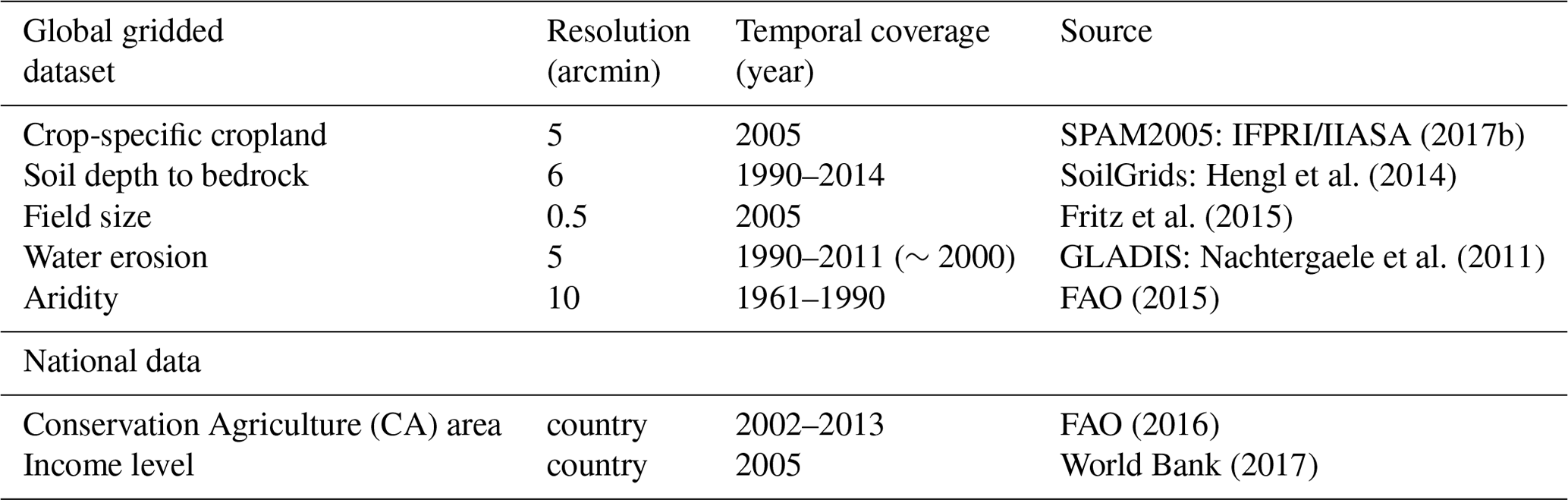
To map the six tillage systems, spatial indicators on the basis of several environmental and socio-economic datasets are applied (Table 2). The basic data layer to this mapping study is the cropland dataset by the spatial production allocation model further referred to as SPAM2005 by the International Food Policy Research Institute and International Institute for Applied Systems Analysis (IFPRI/IIASA, 2017b). It reports physical cropland area for 42 crop types (Table S2 in the Supplement for a list of crop types) for the year 2005. SPAM2005 is a result of a disaggregation of national and sub-national data sources in a cross-entropy approach. The SPAM2005 dataset comprises four technology levels of crop production, distinguishing high input irrigated from purely rainfed with further distinction of rainfed into high input, low input, and subsistence production per crop type and grid cell (You et al., 2014). In this study only the entire physical cropland and the separated irrigated and rainfed cropland were used per grid cell. Adding up the reported cropland area of SPAM2005 for 42 crop types results in a total sum of 11.31 Mkm2.
Table 2Gridded and national-scale datasets used for mapping tillage.
The grid cell allocation key to countries accompanying the SPAM2005 cropland dataset (IFPRI/IIASA, 2017a) was applied in this study for any grid cell aggregation to country scale. Sub-national aggregations of grid cells to state or province level were done with the Global Administrative Areas database (Global Administrative Areas, 2015).
The dataset on soil depth to bedrock (Hengl et al., 2014) has been retrieved from SoilGrids, which is a soil information system reporting spatial predictors of soil classes and soil properties at several depths. It has been derived on the basis of the United States Department of Agriculture (USDA) soil taxonomy classes, World Reference Base soil groups, regional and national compilations of soil profiles, and several remote sensing and land cover products using multiple linear regressions. The dataset reports on the absolute depth to bedrock (centimeters) per grid cell.
The global gridded field size dataset by Fritz et al. (2015) has been derived and validated on the basis of a crowd-sourcing campaign. It reports four field size classes as “very small” (smaller than 0.5 ha), “small” (0.5 to 2 ha), “medium” (2 to 100 ha), and “large” (larger than 100 ha) (Herrero et al., 2017) for the year 2005. The field size and the SPAM2006 datasets both use the cropland extent presented in Fritz et al. (2015).
The Global Land Degradation Information System (GLADIS) (Nachtergaele et al., 2011) reports land degradation types and their spatial extent around the year 2000. From this database the global gridded water erosion data have been selected. The water erosion data report the sediment erosion load (t ha−1 yr−1) per grid cell which the authors derived by applying the Wischmeier equation (Wischmeier and Smith, 1978). Values of the data range from 0 to 12 110 t ha−1 yr−1, with the highest water erosion levels occurring in mountainous areas.
The aridity index dataset was retrieved from the Food and Agriculture Organization Statistics (FAO, 2015). The aridity index was calculated as the average yearly precipitation divided by the average yearly potential evapotranspiration (PET), based on Climate Research Unit (CRU) CL 2.0 climate data averaged for the years from 1961 to 1990 applying the Penman–Monteith method. It reports values per grid cell ranging from 0 to 10.48, where values smaller than 0.05 are regarded as “hyper arid”, 0.05–0.2 as “arid”, 0.2–0.5 as “semi-arid”, 0.5–0.65 as “dry humid”, and values larger than 0.65 as “humid”.
The AQUASTAT online database reports annually the spread of Conservation Agriculture (CA) practices at the national scale (FAO, 2016). From this data source, national CA area values were retrieved for all 54 countries that reported any CA with the total area sum of 1.1 Mkm2. Not all of these countries reported values for the year 2005, so that values closest to 2005 were selected from the available set, giving preference to data availability over matching the year 2005.
The average farm size per country dataset (n=133) (Lowder et al., 2014) is based on FAO farm size time series data. National average farm size was largest in land-rich countries, with the top three countries being Australia (3243.2 ha), Argentina (582.4 ha), and Uruguay (287.4 ha) (Lowder et al., 2014). The authors found average farm size to increase with the elevated income level of a country.
Furthermore, we retrieved the income level per country by the World Bank (2017) for the year 2005. The data refer to four categories of countries' gross national income (GNI capita−1 yr−1), as “Low income” (less than USD 875), “Lower middle income” (USD 876–3465), “Upper middle income” (USD 3466–10 725), and “High income” (more than USD 10 725).
2.3 Processing of input data and mapping rules
For calculation purposes, all gridded input datasets mentioned above were harmonized in terms of spatial extent, resolution, and origin. The spatial extent of the target dataset comprises all cropland cells reported by SPAM2005 (IFPRI/IIASA, 2017b). The targeted resolution is 5 arcmin, which partially required resampling and (dis)aggregation of the applied datasets using R (R Development Core Team, 2013) version 3.3.2 loading packages “raster” (Hijmans and van Etten, 2012), “fields” (Nychka et al., 2016), and “ncdf4” (Pierce, 2015). More details on the input data harmonization and processing can be found in the accompanying R code (Porwollik et al., 2019a).
We developed several mapping rules to allocate the six tillage systems to the grid-cell scale, employing a decision tree as shown in Fig. 1. The decision tree approach has also been applied in other spatial mapping exercises, e.g., in Verburg et al. (2002) and Waha et al. (2012). Hierarchical classification procedures based on expert rules can be used to distribute data of a larger spatial (e.g., administrative) unit to the grid cell level (Dixon et al., 2001; Siebert et al., 2015; van Asselen and Verburg, 2012; van de Steeg, 2010).
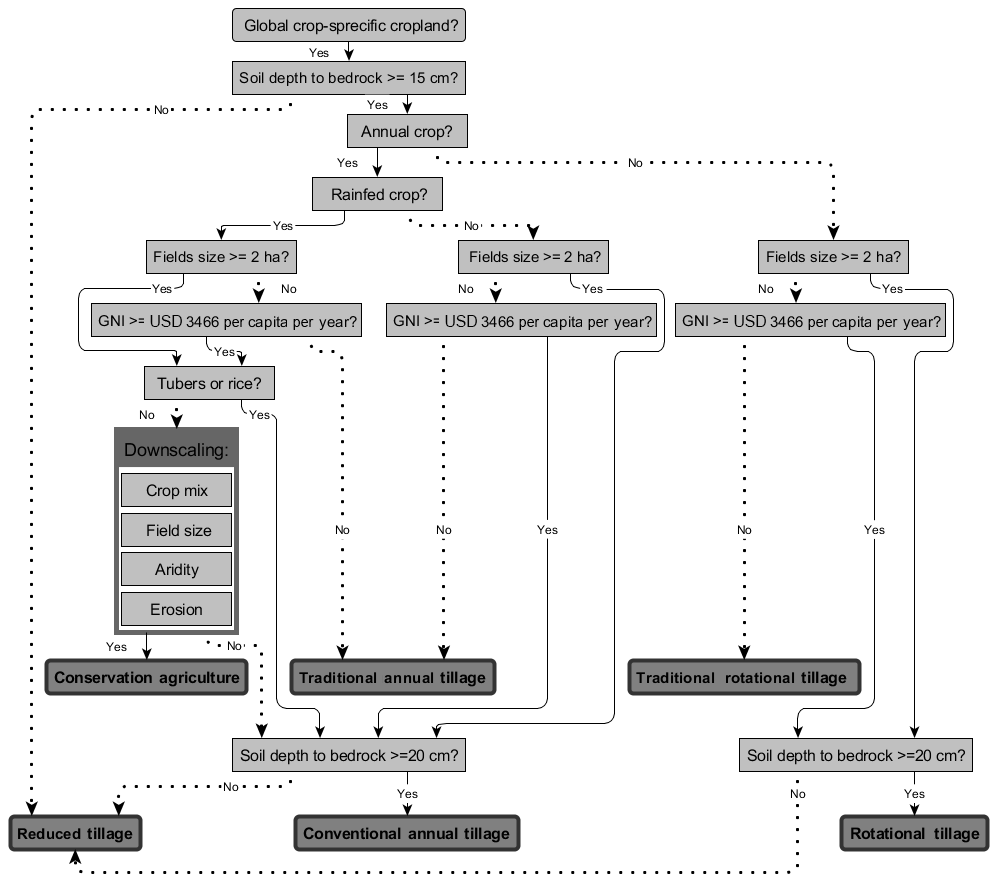
Figure 1Decision tree for allocating cropland to six derived tillage systems. The data processing and mapping were pursued as depicted from top to bottom of the diagram. Each box represents a check on a grid cell of whether reporting values from the different data layers meet the derived thresholds or specific cropland features. The arrows with solid lines indicate a “yes” and arrows with dotted lines a “no” in the allocation procedure of crop-specific area to tillage systems. The box indicating the “Downscaling” represents our probability and suitability indicators applied to downscale national CA area values to a spatially heterogeneous pattern at per grid cell. Boxes with darker grey background shading and thicker frames show the derived types of tillage systems. (Abbreviation of gross national income as GNI).
As a first step, the SPAM2005 cropland dataset is masked for grid cells reporting cropland but soil depth to bedrock of less than the required 15 cm for agricultural production according to Pimental and Sparks (2000) (Fig. 1). This contextual mismatch between these two datasets may be caused by different input data used by the producers or by their method of averaging values within one grid cell, in which the soil depth to bedrock is heterogeneous. The entire cropland of these shallower grid cells is allocated directly to the reduced tillage system area, where ridging or raised beds may be practiced by the farmer because of physical hindrance for inverting tillage practices at increased depth.
The remaining cropland is treated separately for annual and perennial crops following Erb et al. (2016)'s findings, differing between plant-type associated tillage by intensity in terms of frequency and timing of the tillage operation (Table S2 for crop-type classification).
As a further step, we distinguished tillage practices per water management regime. We assumed that soils of irrigated crops are more regularly exposed to some level of mechanical soil surface alteration, i.e., leveling off of the surface in order to distribute irrigation water most efficiently and homogeneously over the field. We allocated all irrigated annual cropland either to traditional or conventional annual tillage area depending on field size and income level (Fig. 1).
Annual and perennial tillage systems are both further distinguished by the level of mechanization and commercial orientation of the crop production. We follow the definition of smallholder farming used in Lowder et al. (2016) if cultivation area is smaller than 2 ha. According to Fritz et al. (2015), field size can be regarded as a proxy for agricultural mechanization and human development. Further, Levin (2006) found that field size and farm size are positively related. Based on these findings, we apply the field size dataset as a proxy for farm size and mechanization. We categorize cropland per grid cell reporting field size equal to or larger than 2 ha as “large” scale assuming access of the farmer to mechanized farming equipment, and field size smaller than 2 ha as “small” scale farming with rather manual labor. Field size data are not available for all grid cells where SPAM2005 reported cropland. Consequently we interpolated for missing field size grid cell values using the mean of surrounding grid cell values. The spatial distance to the Hawaiian islands was too far for this operation, so there field size was set to a value of 2 ha, assuming a land restriction to field size due to the islands' geographic pattern and in the absence of any alternative information.
We further assume that animal draught power and mechanized soil management practices on a farm also occur as a function of income, indicating the financial capital a farmer might have access to. Therefore, we additionally apply the national average income level dataset to differentiate between small field sizes in higher-income countries, where access to financial capital for investment in farm equipment is perceived to be easier than for farmers with small field sizes in lower-income countries. In order to do so, we reclassified countries reported in the income dataset considered “low” and “lower-middle income” as “low income”, and those countries formerly considered “upper-middle income” and “high income” as “high income”, in this study. In grid cells reporting newly derived small field size and low income, we then allocated perennial cropland to traditional rotational tillage and annual cropland to traditional annual tillage. In high-income countries or in a grid cell reporting field sizes larger than 2 ha situated in low-income countries, perennial cropland was assigned to rotational tillage and annual cropland to conventional annual tillage assuming a rather commercially oriented farming system with access to market, financial capital, and therefore mechanized soil management equipment (Fig. 1).
We applied a downscale algorithm of national reported CA area values to a subset of rainfed annuals' cropland area (see Fig. 1, box “Downscaling”; see the following Sect. 2.4 for more details). The remaining rainfed annuals' cropland not being assigned to CA area is checked again for soil depth to bedrock. In case it was shallower than 20 cm, the cropland was also assigned to reduced tillage, assuming less depth, frequency, mixing efficiency, or alternative cultivation practices. In the case of a soil depth to bedrock of 20 cm or more, the remaining cropland depending on crop type was either mapped to the conventional annual or to the rotational tillage system.
2.4 Downscaling reported national CA area to the grid cell
2.4.1 Mapping rules for downscaling CA
Generally it can be assumed that the entire cropland is suitable for some kind of sustainable farming technique, but in the following we refer to “potential CA area” as the area where we regard the adoption of CA as more likely than for the remaining cropland where CA adoption would require additional assistance or support for the farmer. Potential CA area is derived from the cropland of 22 rainfed annual crops in grid cells reporting dominant large field size in low-income countries and all field sizes in high-income countries. Cropland areas of annually planted rainfed crop types were considered suitable for CA practice following the finding of Kassam et al. (2009), who state that much of the CA development to date has been associated with rainfed arable crops. We selected the following annual crop types reported by SPAM2005 as suitable for CA in this study: barley, beans, chick peas, cotton, cowpea, groundnut, lentil, maize, other cereals, other pulses (e.g., broad beans, vetches), pearl millet, pigeon pea, rapeseed, rest (e.g., spices, other sugar crops), sesame seed, small millet, sorghum, soybean, sunflower, tobacco, vegetables (e.g., cabbages and other brassicas), and wheat (see Table S2), following Giller et al. (2015)'s findings on CA suitability of (dryland) grain crop types. All annual rainfed root, tuber, and rice cropland is excluded from the potential CA area following Pittelkow et al. (2015), who reported larger yield penalties for these crop types when applying no-tillage practices. Rice is often produced as paddy rice, requiring puddling, which is a practice modifying the soil aggregates a lot in order to facilitate the flooded condition, e.g., to suppress weed growth. A conversion from puddled to dryland rice production as well as improved drainage of tuber crop production area may require additional management steps by the farmer in order to achieve comparable yield levels with no-tillage to under conventional production methods. The resulting potential CA area amounts to 4.65 Mkm2.
As stated by Powlson et al. (2014) for the Americas and Australia, by Rosegrant et al. (2014) in general on no-tillage, by Scopel et al. (2013) for Brazil on CA, and by Ward et al. (2018) on CA, the largest adoption rates of minimum soil disturbance management principles can be found on medium to large farms. There is low adoption of CA or no-tillage among small-scale farms, with the exception of Brazil (Rosegrant et al., 2014), where adoption of CA was supported through policies and technological investments.
We developed a linear regression with the “stats” package of R (R Development Core Team, 2013), applying the linear correlation model (“lm function”) to assess the statistical relation between national average farm size (Lowder et al., 2014) and percentage share of CA area (FAO, 2016) on arable land. The functional relation exhibits an increase in the national share of CA on arable land with an increase in average farm size over the country sample (Fig. S3).
Based on the literature findings and regression results, we assumed that no-tillage in the context of CA was highly probable for cropland in grid cells with large fields (here serving as a spatial proxy for large farm size and mechanization).
Furthermore, we considered no-tillage to be suitable for arable production under arid conditions (Kassam et al., 2009; Pittelkow et al., 2015), because of less aeration, more stable pores, and soil aggregates compared to soils managed with conventional tillage. In CA systems, the evapotranspiration is additionally reduced by a continuous biomass cover of at least 30 % of the soil surface, which promotes yield stability in drought-prone production environments.
As a last allocation criterion, CA was regarded as suitable for crop production in areas with elevated erosion levels. Basso et al. (2006) find that farmers may make use of green or residue cover to protect the soil surface during high-intensity rainfall events. Our mapping rule too is in line with the finding of Kassam et al. (2009) stating that wind and water erosion were major drivers of CA adoption in Canada, Brazil, and the USA. According to Schmitz et al. (2015) and Govaerts et al. (2009), Asian and African agricultural producers could also benefit from the positive effects of CA in erosion-prone areas.
2.4.2 Logit model for downscaling national CA
Cropland, field size, water erosion, and aridity data per grid cell are used as predictors determining the spatial distribution of national reported CA area within a country (Fig. S4.1–4). We developed a logit model to transform and combine these four spatial predictors into probability values per grid cell, indicating the likelihood of CA area occurrence. The logit model was chosen because different ranges of the spatial predictor datasets are made comparable at equal weights without losing much detail.
From the potential CA area data layer we computed the input variable “crop mix” as the ratio of the area sum of 22 CA-suitable crop types over the sum of total cropland area per grid cell. We assume an increasing probability for CA area occurrence in grid cells with an increasing cultivated area share of CA-suitable crop types. This was based on the assumption that cropland within a grid cell belongs to one management regime under which rotations with CA-suitable crops are practiced and a similar set of soil working equipment is employed. The assumptions also takes into account peer group influence and knowledge spillover effects from early adopters of a new technology (here CA practice) on their neighbors (Case, 1992; Maertens and Barrett, 2013).
Regarding the statistical relation between farm size and CA adoption, we assume that the larger the field size, the higher the CA probability, especially for field sizes equal to or larger 2 ha depending on the income level of a country, taking 2 ha as the midpoint of the transformed field size logit curve.
We set missing water erosion values in grid cells reporting potential CA area to the neutral value of 12 t ha−1 yr−1, since it depends on very small-scale conditions, e.g., slope. When transforming the water erosion values to logit, we set 12 t ha−1 yr−1 as the midpoint value of the function. Here the corresponding mapping approach was to assume increased probability of CA practices in cells which report water erosion values exceeding 12 t ha−1 yr−1 as the upper bound of the soil loss tolerance value (T-values) defined by the USDA (Montgomery, 2007).
The midpoint of aridity's logit regression curve is chosen at 0.65, resulting in higher probabilities of CA area occurrence for grid cells reporting arid (values smaller than 0.65) rather than humid (values larger than 0.65) growing conditions. We interpolated missing aridity values in grid cells where SPAM2005 reports cropland, except for one island near Madagascar, which we set to the logit-neutral value of 0.65 because we assumed very special climatic conditions there.
We tested for (Pearson) correlation among the four spatial predictor variables with the R “base” package (R Development Core Team, 2013), in order to prevent autocorrelation effects (Table 3).
Table 3Correlation coefficients (r) according to Pearson between spatial predictor variables (crop mix, field size, erosion, and aridity) across all grid cells containing potential CA cropland globally.

Generally correlation coefficients (r) among the datasets are low and mostly negative, except for field size and crop mix.
Those four cropping system indicators are used as explanatory variables in the regression to get the probability of cropland in a grid cell to be CA area as a value between 0 and 1. The probability of CA in a grid cell is derived via the following Eq. (1):
where i represents the input datasets of water erosion, aridity, crop mix, and field size (proxy for farm size), ki refers to the slope value, xmidi to the central points of each of the logit curves, and vxi to grid cell values of the referring input dataset.
A sensitivity analysis has been conducted to assess the explanatory power of each of the four input variables and the uncertainty of our parameter set and combination (Fig. S5). The first step was to vary our chosen reference slope (ki) of each of the input dataset values by factors of 2 and 0.5 (+100 %, −50 %). As a next step each of the variables is dropped, and finally each of the variables is used individually in the logit model. The sensitivity test was conducted at the global scale and also for each of the 54 CA reporting countries.
2.4.3 Mapping CA area per country
The downscaling of total national CA area values entailed subsetting all grid cells with CA-suitable area per CA area reporting country (FAO, 2016). Then these grid cells were sorted in decreasing order according to their CA probability values derived with the logit equation. As a next step, grid cells with the highest logit model results were selected step-wise while adding up the corresponding potential CA area until the reported national CA area threshold was reached. We received a heterogeneous pattern of allocated CA area at 5 arcmin resolution grid within a CA reporting country according to the likelihood of CA area occurrence based on the logit results, statistical data, and literature findings.
2.4.4 Scenario CA area
Similar to the “bottom-up scenario” of Prestele et al. (2018), we deduced “scenario CA area” indicating the maximum area extent of CA adoption, under assessed current socio-economic and biophysical conditions. We add the subset of 22 annual rainfed crop-specific areas in grid cells with large field sizes in low-income countries and all field sizes in high-income countries from reduced tillage to the potential CA area to calculate scenario CA area per grid cell.
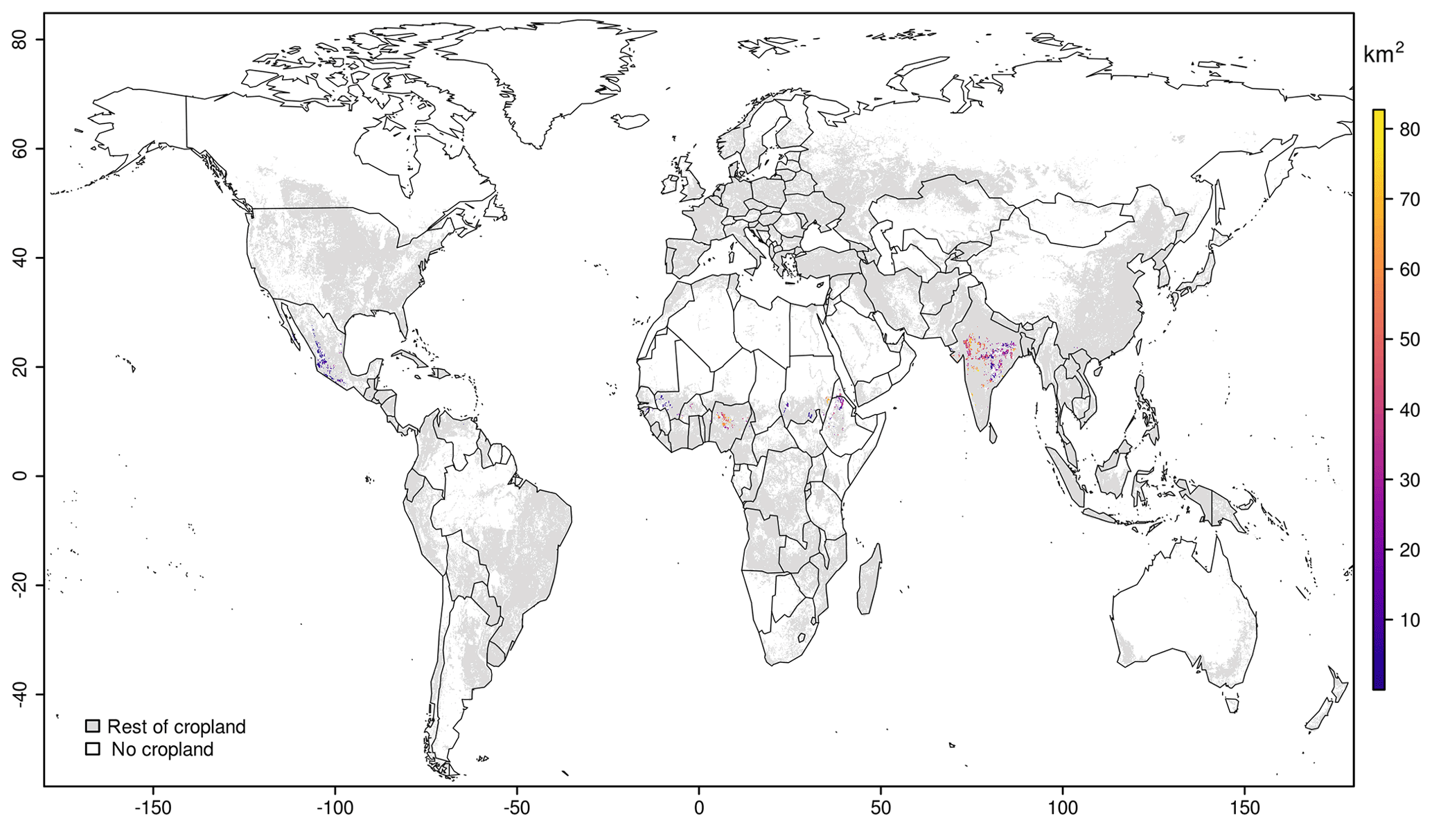
We allocated global cropland of SPAM2005 to the six tillage systems at a spatial resolution of 5 arcmin according to a set of rules (Table 4). In terms of area, conventional (Fig. 2) and traditional (Fig. 3) annual tillages globally constitute the most widespread tillage practices. Both systems are applied for annual crops, which are globally growing on the largest cropland fraction, are traded, and are consumed most. Large parts of the cropland under traditional annual tillage for rainfed and irrigated annuals are located in South-East Asia, with especially high cropland area shares in India followed by sub-Saharan Africa and then South America (Table S9 for aggregated tillage system areas to country scale). Conservation Agriculture globally constitutes the third largest tillage system area (Table 4 and the following Sect. 3.1). Rotational tillage (Fig. 4) is in fourth position in the ranking of tillage system areas, followed by traditional rotational tillage area (Fig. 5). Most traditional rotational tillage system area can be found across the tropical region of South-East Asia and western Africa. Reduced tillage has the smallest area extent (Table 4), which we find mostly in a narrow band between 10 and 20∘ northern latitude (Fig. 6). It occurs in Mexico and south of the Sahel region, but mostly is found on cropland in India (Table S8 for further metrics across tillage system areas; Table S9).
Table 4Global aggregated tillage system areas and shares on total cropland (IFPRI/IIASA, 2017b).
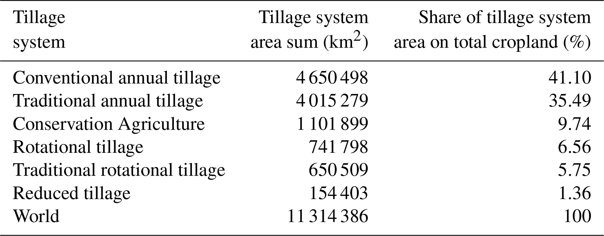
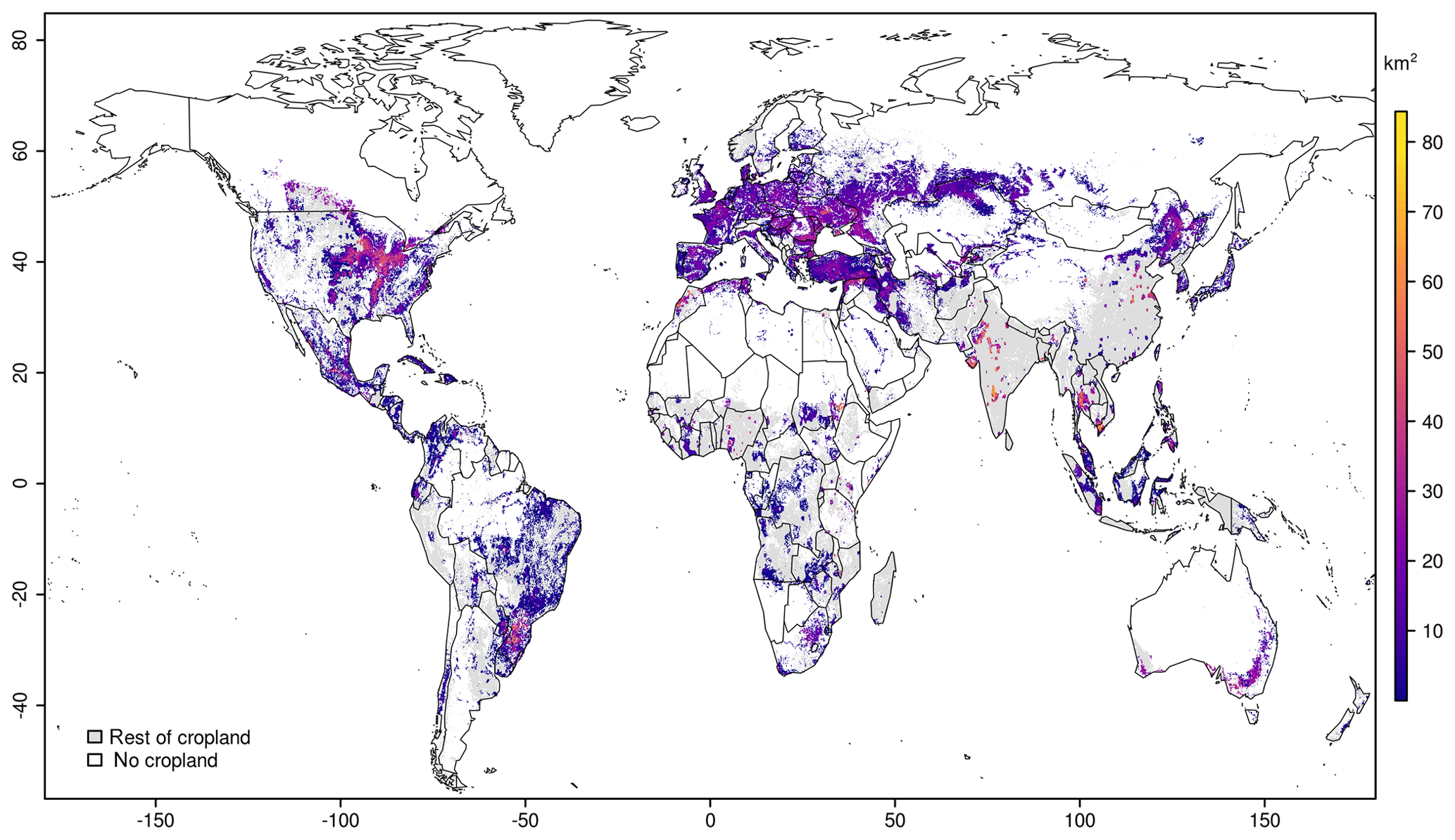
Figure 2Conventional annual tillage area, which has been allocated to the majority of the global physical cropland area.
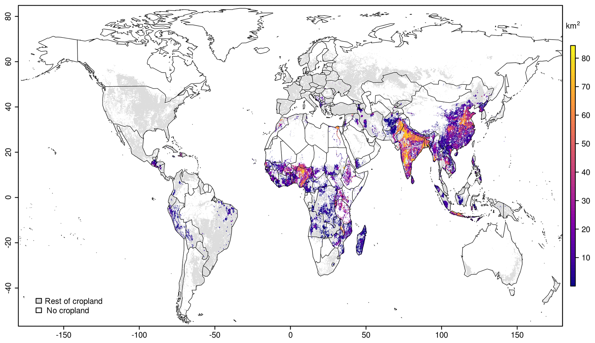
Figure 3Traditional annual tillage area as sums over 29 annual crop types' areas in grid cells reporting dominant field sizes smaller than 2 ha and in countries classified as low income in this study.
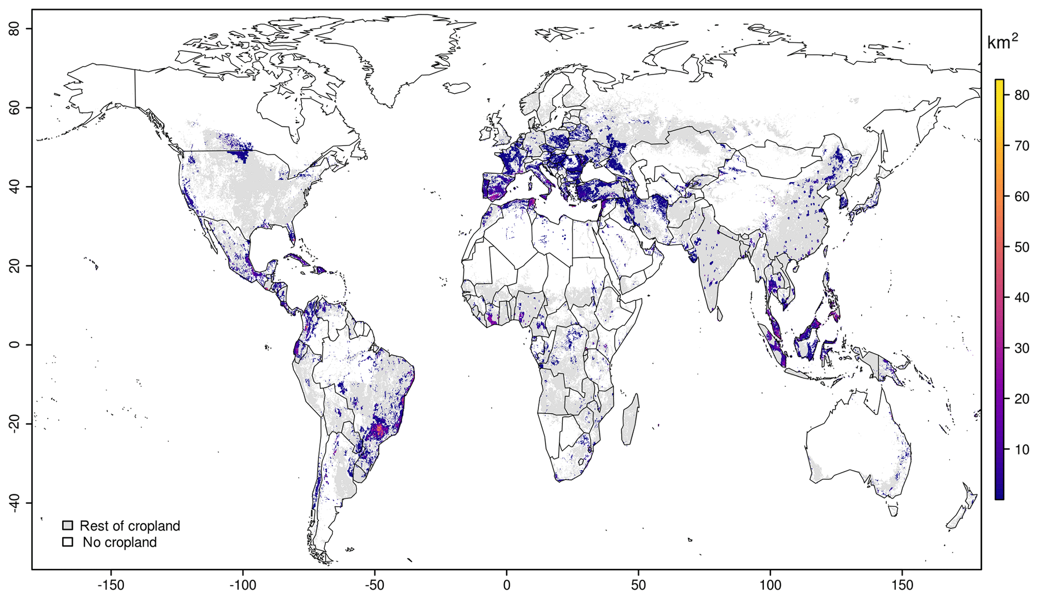
Figure 4Rotational tillage area on cropland area of 13 perennial crop types in grid cells with dominating field sizes of minimum 2 ha or larger in low-income countries or all field sizes in high-income countries.
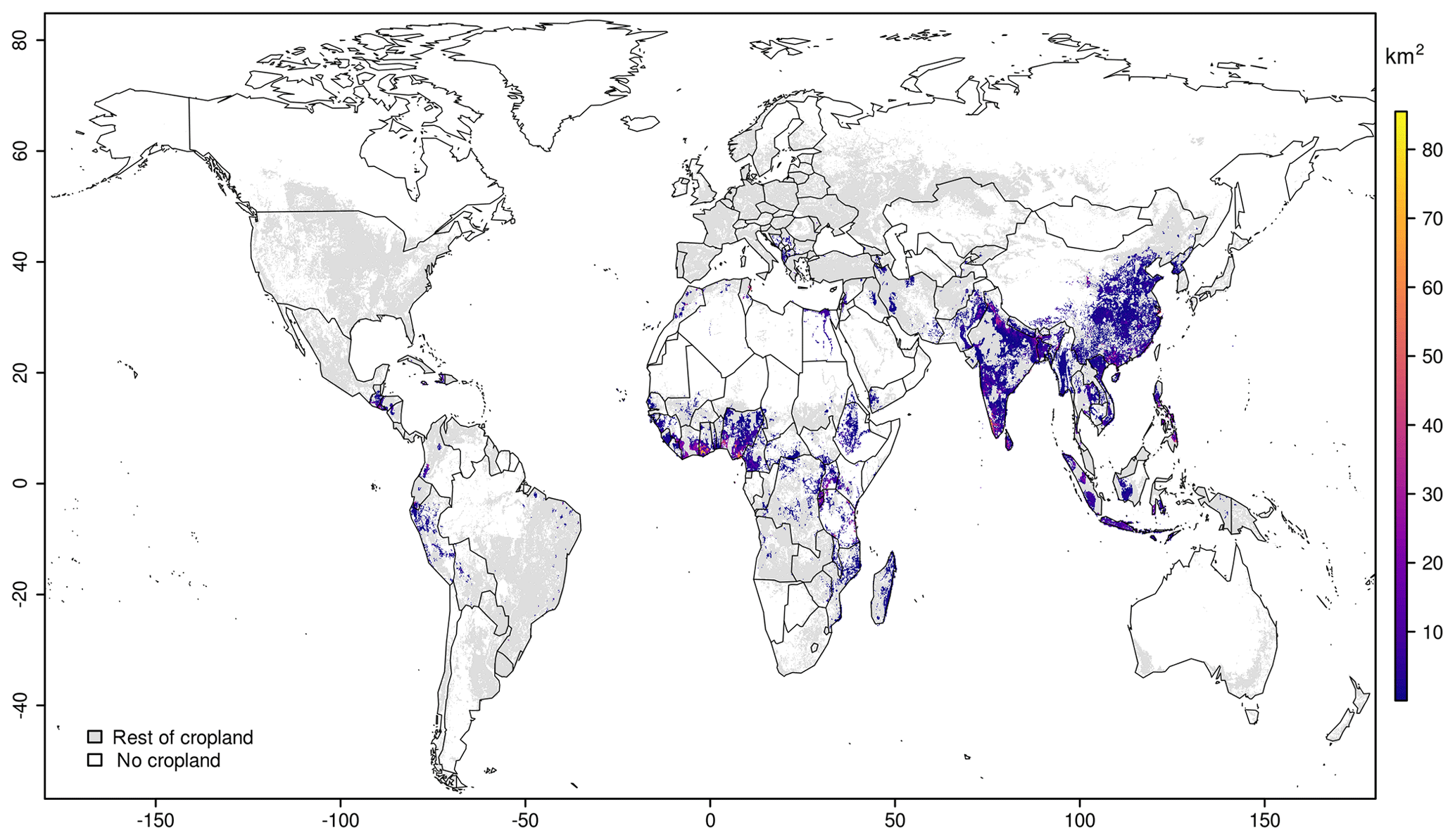
Figure 5Traditional rotational tillage area as cropland of 13 perennial crop types in grid cells characterized by field sizes smaller than 2 ha in countries considered low income in this study.
3.1 Conservation Agriculture area
3.1.1 The results of the logit model
We deduced the likelihood of CA area in a grid cell via the logit model approach according to the indicators crop mix, field size, water erosion, and aridity (Fig. 7). The geographical pattern of the logit results (further referred to as ref-logit) exhibits higher probabilities for cropland in grid cells outside the tropical climate zone and in rather continental regions. Probability of CA is higher for cropland in grid cells reporting large field sizes, which are mostly found in developed and land-rich countries, i.e., in the USA, Australia, and large parts of Europe. Grid cells in the tropics receive rather low logit results due to their humid conditions, smaller field sizes, lower income levels, and crop types cultivated. In India, China, and Pakistan the majority of cropland showed very low CA likelihood.
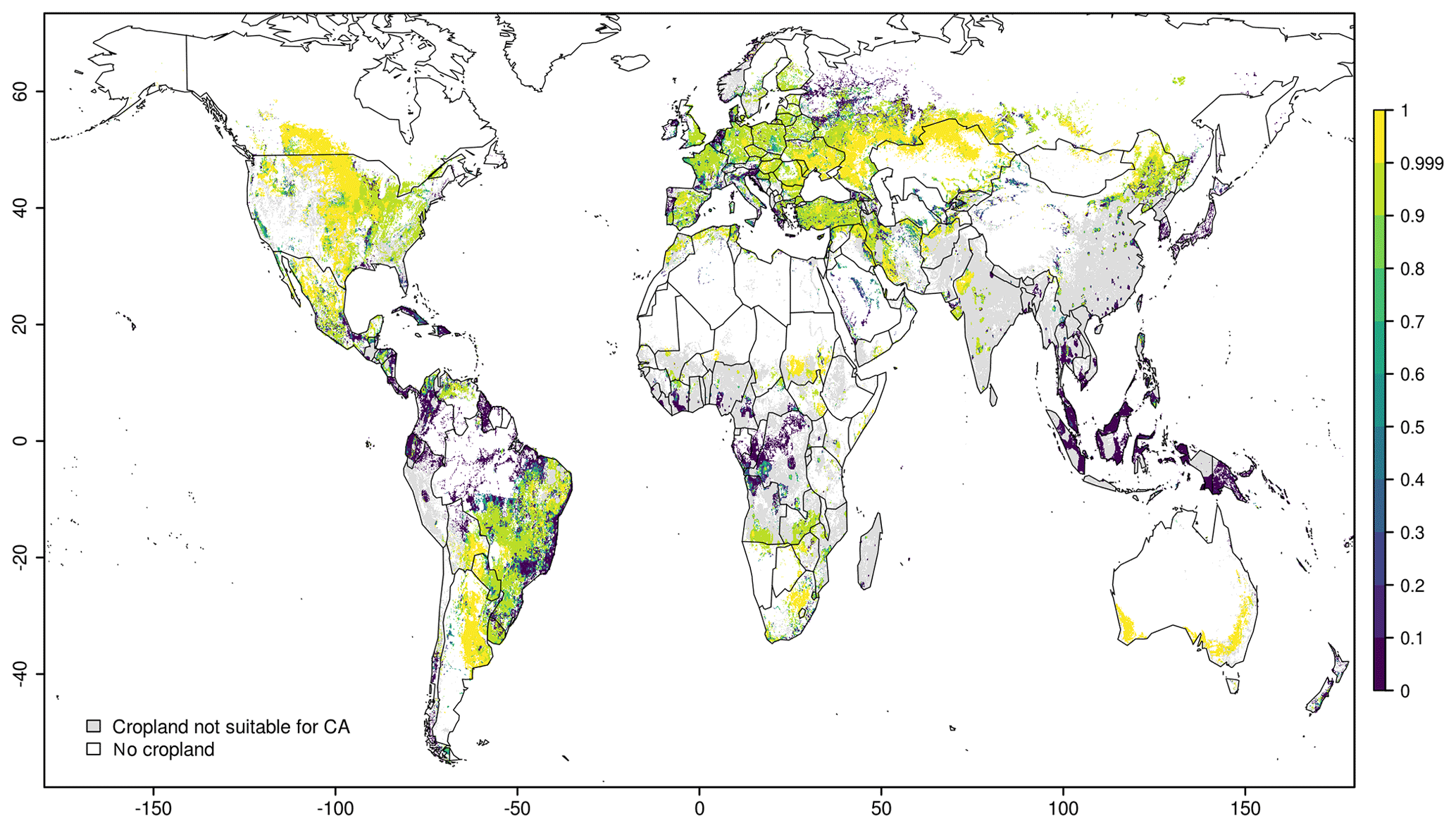
Figure 7Probabilities of Conservation Agriculture area per grid cell with high values as green to yellow and low ones in blue to purple colors (white color indicates the absence of cropland, and grey the cropland (IFPRI/IIASA, 2017b) which is excluded from the potential CA area due to soil depth, crop type, irrigation, field size, or income level).
3.1.2 Results of the sensitivity analysis of the logit model
The sensitivity analysis of the logit model shows mixed responses to the perturbations of slope or variable combination (Table 5, Fig. S5). Rank correlation (r) to the ref-logit is much lower when taking one variable only compared to each of the other drop-variable settings or slope modifications. Regarding modifications of the slope parameters of the input variables, we calculated the lowest rank correlation coefficient for increasing the slope of aridity by +100 % and for decreasing the slope of crop mix by −50 % compared to changing the slopes of the other three variables, respectively.
Table 5Logit model input parameters, as midpoint (xmid) and slope (k) of the four logit model input datasets (columns 1 and 2), which are altered per sensitivity setting. Correlation coefficients (r) for ranks according to “Spearman” between the reference case (Logit-ref) and the perturbed slope and variable combinations of the logit model results are given, illustrating the sensitivity of the grid cell likelihood of potential CA area (columns 3 to 6).
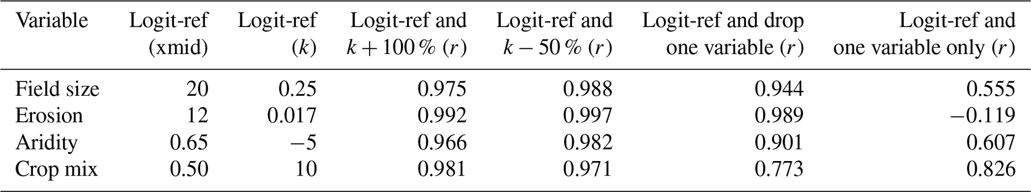
Erosion has the lowest explanatory power, as can be interpreted from the very high correlation coefficient with ref-logit when dropping it – but even negative correlation when taking it into the logit equation only. This finding is in line with the findings of the sensitivity tests performed by Prestele et al. (2018), who find erosion to be the variable with the smallest explanatory power as well.
Crop mix has the largest explanatory power in the logit equation, as shown by the lowest correlation coefficient value when dropping it but highest when taking that variable only (Table 5). We additionally report on the sensitivity results for the 54 CA reporting countries, where the effects of slope and variable perturbation show very different patterns per country (Table S6). However, as national CA areas are allocated within individual countries, the sensitivity of ranking within countries is of greater importance than the global rank correlation.
3.1.3 Downscaled CA area
Total downscaled CA area (1 101 899 km2, Fig. 8) is slightly lower than FAO reported total CA area for these countries (1 102 900 km2). This difference occurs because of our algorithm, which assigned the entire CA-suitable cropland area per grid cell to CA, taking the cropland of the following grid cell in or out of consideration striving for least deviation from the threshold per country (Table S7 for comparison of reported and downscaled country values). A further difference is due to the insufficient potential CA area in North Korea and New Zealand, resulting in the fact that only part of the national reported CA area could be allocated to.
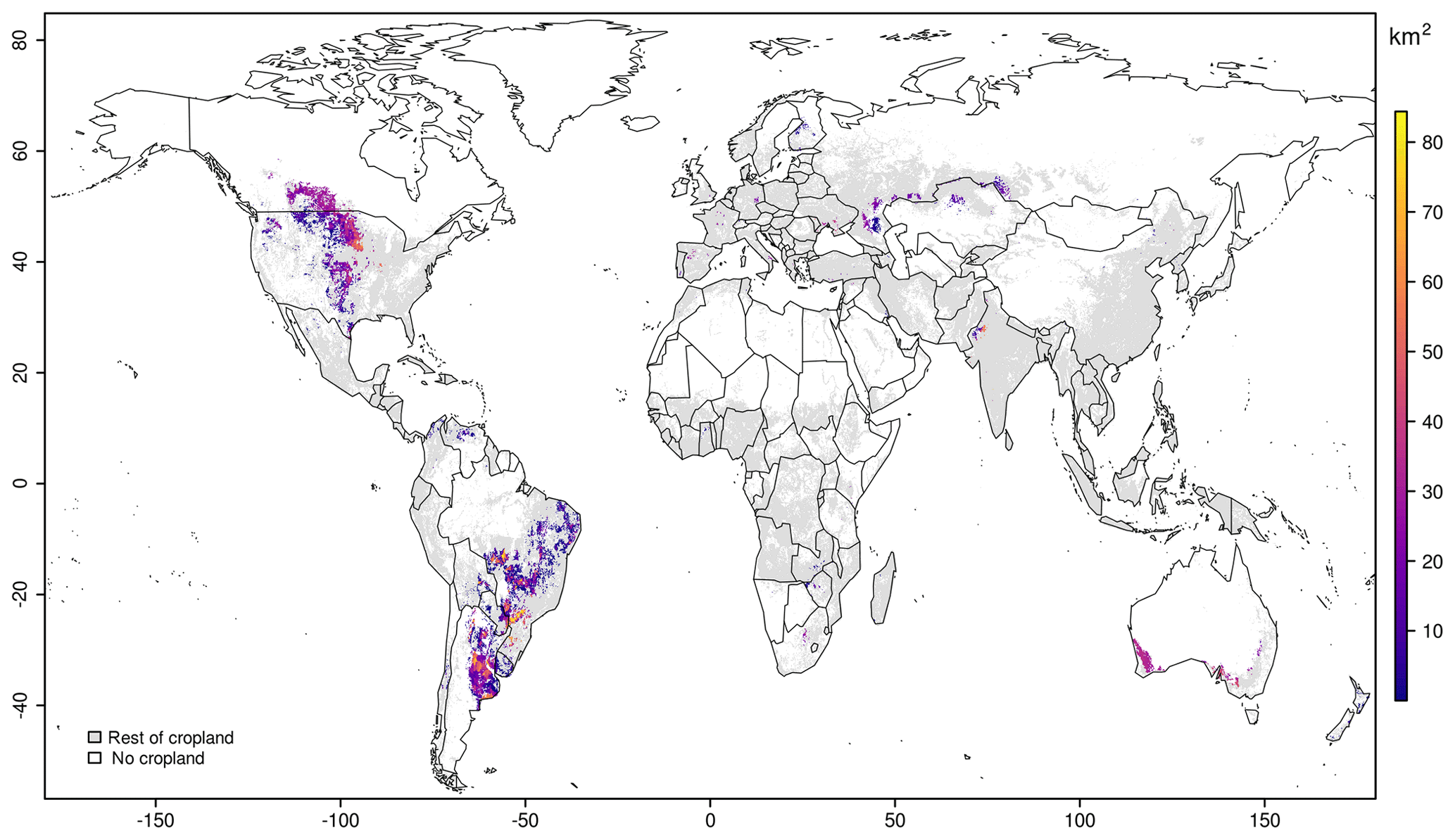
Figure 8Downscaled Conservation Agriculture area (km2) (colored) on total cropland (grey) per grid cell for 54 reporting countries around the year 2005.
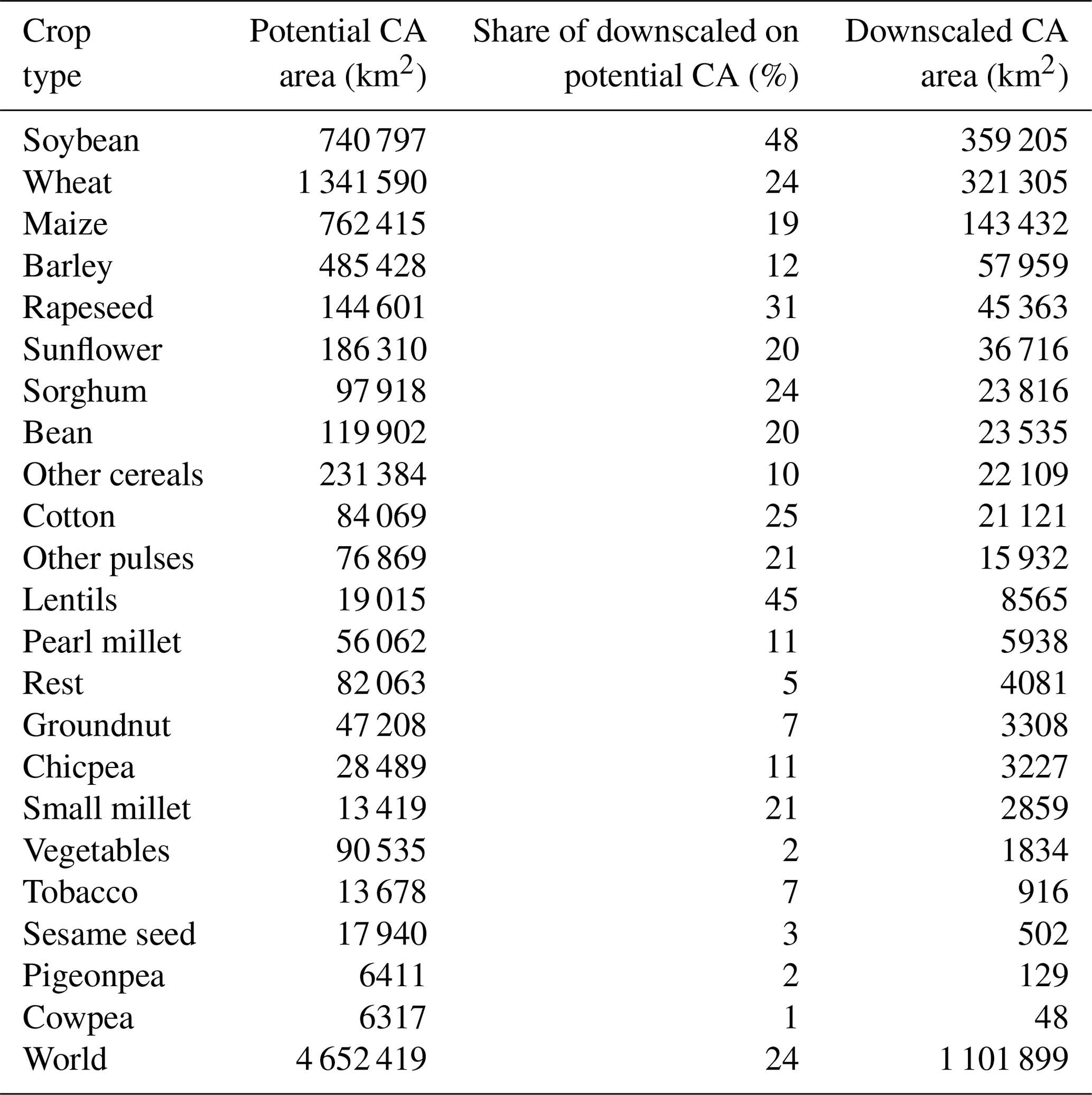
Aggregated crop-specific CA area values reveal that most downscaled CA area was allocated to area cultivated with soybean, followed by wheat and then maize (Table 6). These three crops are among the most important produced, traded, and consumed agricultural goods, making their production highly competitive, and therefore the incentive to reduce operational costs (e.g., regarding tillage) is high. Another reason for soybean and maize being among the crops mostly produced under CA may be the usage of high yielding or genetically modified crops, coming along with improved pesticide resistances, which make them more suitable for possible herbicide applications (Giller et al., 2015) replacing tillage operations on-field. In Argentina, soybeans are found to be the most common plant cultivated under CA, with usually lower residue coverage than required for being a CA system (Pac, 2018). Subsistence farming crops, e.g., peas and millet, contributed only a little cropland to the downscaled CA area (Table 6), because they are more drought resistant (Jodha, 1977), and of rather regional importance in terms of food security, while being traded less on the international markets (Andrews and Kumar, 1992).
Table 6Global sums over 22 CA suitable crop-type areas, sorted decreasing shares of downscaled CA area values on the identified potential CA area, and crop-specific downscaled CA areas.
3.1.4 Scenario CA area
We deduced the total global potential CA area of 4.65 Mkm2 (see above). Additionally, we identified 0.02 Mkm2 of 22 rainfed annual crop types' areas on large fields in low-income countries and all field sizes or in high-income countries from the reduced tillage system area, which potentially could be converted to CA area as well. We calculated a total scenario CA area of 4.67 Mkm2, where perceived driving forces, e.g., CA adoption supporting agricultural policies, targeted mechanization efforts, and knowledge dissemination approaches could lead to an area expansion of CA practices.
The presented tillage system dataset and source code are available under the ODBL (data) and MIT (source code) licenses. The tillage dataset can be downloaded from https://doi.org/10.5880/PIK.2019.009 (Porwollik et al., 2019b) and the corresponding R-code from https://doi.org/10.5880/PIK.2019.010 (Porwollik et al., 2019a). The dataset is provided in netCDF format (version 4) and consists of 42 layers, each reporting crop-specific tillage systems per grid cell. Additionally, we provide a layer indicating area, where adoption of Conservation Agriculture could be facilitated (scenario CA area). The dataset can be used as a direct input or be applied as a mask or overlay for identifying tillage area. The R-code is provided to increase the transparency of our methods, but also to enable other modeling groups to adjust our tillage area mapping algorithm to their needs, e.g., for different input data or scenarios.
5.1 Comparison of results to other studies
In the absence of alternative tillage area datasets for validation at the global scale we here want to discuss the way our tillage system area results relate to other studies' findings.
We compare the spatial pattern of our added traditional tillage system area to the one reported by the cropland subsets of SPAM2005 for low-input and subsistence production. According to You et al. (2014), both production levels are characterized by a low level of mechanization, or rather manual labor and low input usage. The sum of our traditional tillage systems' (rotational and annual) areas (4.63 Mkm2) is slightly higher than the sum of SPAM2005 subsistence and low-input technological-level cropland (4.55 Mkm2). We deduced more traditional tillage system area in South-East Asia, Sub-Saharan Africa, and Peru than SPAM2005 reported under low and subsistence farming (see the difference map in Fig. S10). Further comparison reveals a moderately lower amount of area under traditional tillage in our dataset for Europe, the Middle East, South America, and Australia, i.e., in countries which are regarded as emerging or developed economies. The spatial difference may be due to the fact that SPAM2005 is a product of a sub-cell cross-entropy optimization approach to distribute cropland of the same crop species into several production levels per grid cell. In contrast to this, we used the field size and gross national income as spatial indicators of un-mechanized tillage systems by masking out cropland either per entire grid cell or country-wise according to our derived thresholds. We calculated the spatial correlation via a regression of the added area values of our traditional tillage system and of the sum of low-input and subsistence production level cropland reported by SPAM2005. We found a regression factor (r2) of 0.54 (p<0.001, slope of 1.139) among both datasets' values.
Our estimate of a traditional tillage system area in turn is lower than the finding by Lowder et al. (2016), stating 5.87 Mkm2 to be under management of farms smaller than 2 ha in size (∼12 % of their arable cropland assumption).
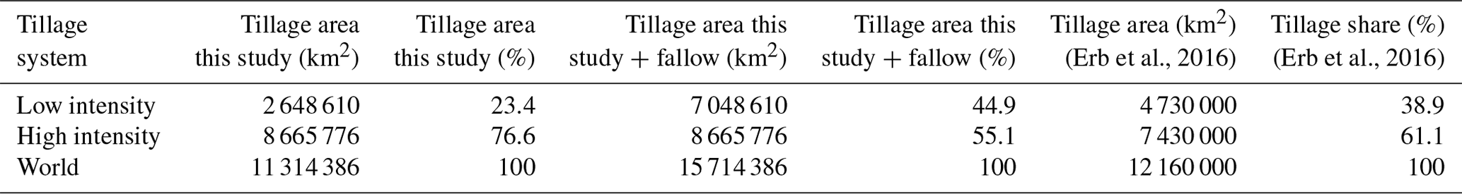
In order to compare our results to the findings of Erb et al. (2016) on tillage intensity areas, we added up our reduced, both rotational tillage system, areas, and the downscaled CA area to represent the “low intensity” tillage area, whereas conventional and traditional annual tillage are summed up to the “high intensity” tillage area. Since the description of what is included in their “low intensity” area is inconsistent within their main text, tables, and Supplement, we state two different estimates of our results – both exhibiting different absolute values and shares compared to the findings of Erb et al. (2016) (Table 7).
Table 7Tillage system area results compared to estimates of Erb et al. (2016) on tillage intensity areas. The first two columns show our aggregated tillage system area values; columns 3 and 4 additionally include the young and temporal fallow cropland area by Siebert et al. (2010), a cropland area not represented in SPAM2005 and therefore added to our total cropland as well as to the “low intensity” category as described in Erb et al. (2016). Note that Siebert et al. (2010) state that about 4.4 Mkm2 of cropland was young and temporal fallow (<5 years) around the year 2000.
We additionally pursued a provincial- and state-level comparison between our downscaled CA area to reported no-tillage area values for Canada, Brazil, and Australia (Fig. S11 and Table S11), because these countries are among the top four adopters of CA (see Table S7). CA area values from AQUASTAT (FAO, 2016) for these three countries were dated 2006, 2005, and 2006 and compared to reference reporting years of 2006, 2007–2008, and 2006, respectively. Although this provides a comparison to independent data, it cannot be considered a validation because of the temporal mismatch among compared datasets and aggregation uncertainty when using Global Administrative Areas (2015) for aggregating tillage areas to sub-national scale. For each of the selected countries our downscale algorithm can quite well reproduce the main no-tillage area, but tends to too strongly concentrate CA area in some regions instead of a more homogenous spread, as observed in the associated reference maps.

Figure 9Scenario Conservation Agriculture area (km2) (colored) on total cropland (grey) per grid cell.
Prestele et al. (2018) analyzed CA area time series data by FAOSTAT and found an increasing trend of CA adoption within countries and to more countries since the 1970s. This trend is likely going to continue as farm holdings increase in size while decreasing in number in upper-middle- and high-income countries (Lowder et al., 2016). At the same time, the adoption rate of CA in smallholder farming systems in low-income countries (e.g., in Sub-Saharan Africa) may continue to be low, where average farm size reveals a decreasing trend (Jones, 2017). Adoption of CA practices by smallholder farmers is hampered by competition for residue use (Scopel et al., 2013), missing knowledge, as well as restricted access to inputs and financial capital (Kassam et al., 2009), making them more risk-averse towards adoption of new technology than large-scale farmers (Schmitz et al., 2015).
Prestele et al. (2018) state their potential CA area to be 11.3 Mkm2 in their “Bottom-up” and 5.33 Mkm2 in their “Top-down” scenarios until the year 2050. Our estimate of scenario CA area of 4.66 Mkm2 is lower but on the same magnitude as their “Top-down” scenario. Prestele et al. (2018) used another cropland product, targeted another time period, pursued a slightly different CA mapping approach, and had different assumptions about the scenario design, which might be causing the main area differences compared to our derived scenario CA area. In order to take into account that other modeling groups may apply other cropland inputs than SPAM2005 as presented here, we made the tillage dataset and source code flexible in a way that each modeling group may adjust it according to their individual crop mix per grid cell.
5.2 Potentials, limitations, and implications for applications of the dataset
A limitation to our presented mapping approach is that the input datasets applied cover different time periods, e.g., GLADIS reports water erosion values for approximately the year 2000, SPAM2005 and the field size dataset for the year 2005; the aridity spans to the reference climate data of the period from year 1961 to 1990, and for some countries we extracted the only CA reporting year by FAO (2016) from years 2002 up to 2013. By using SPAM2005, field size for 2005, and setting the objected year for the produced tillage dataset to 2005 as well, we tried to minimize inconsistencies in time coverage at least for the cropland extent. GLADIS uses the Global Land Cover dataset (GLC2000, Bartholomé and Belward, 2005) as land-use information, thus reporting water erosion values as an average over the different ecosystem and land-use types per grid cell. Land use as well as land management are results of dynamic socio-economic and environmental processes. Local mismatches in the cropland extents between these datasets might be on the one hand due to abandonment as a result of shifting cultivation or on the other hand due to extension of cropland to converted other land-use types between the years 2000 and 2005. Further mismatches might exist due to different assumptions about crop types and area between different data products. The choice of crop to be cultivated is usually taken under consideration of rotations for weed and pest management, household demand, and market conditions, together leading to different cropping patterns between the years 2000 and 2005. The aridity dataset does not consider any land-use information, but relies on averages of climatic data and parameters. Another source of uncertainty is the used rule-based approach for mapping the tillage system areas. We statistically proved the relation between national average farm size and CA adoption (S3). Whereas statistical relations between field and farm size can be found in the literature, the mapping rules of distinguishing traditional from mechanical tillage and the suitability of CA for erosion and aridity-prone agricultural production environments are based on qualitative literature findings and warrant further research and scrutiny if new data become available.
The tillage dataset presented here can be employed in various applications, depending on the type of model, context, and objective of the user. Agricultural land management practices are determined not only by environmental factors, but are also embedded in local to regional systems of culture, traditions, and markets. This mosaic of farming conditions can only be taken into account at high spatial resolution. The developed tillage dataset is an effort to better account for heterogeneous patterns of agricultural soil management across and within countries by using socio-economic and biophysical data in conjunction. The resolution of the generated dataset of 5 arcmin is quite high. Global ecosystem models are currently mostly run at a coarser resolution than our dataset's resolution, and the tillage data may have to be aggregated in such cases. This could introduce further uncertainty to the area under a certain tillage system.
A challenge to the full usage of this dataset is the limited implementation of the 42 crop types reported in SPAM2005 in global ecosystem models. Especially perennial crop types are hardly ever parameterized in ecosystem models, or if so rather address regional-scale applications (Fader et al., 2015). One reason for the missing implementation may be their relatively small cultivation areas globally (∼10 % of global cropland, Erb et al., 2016). Woody and other perennial plant species entail potential in the aspect of sustainable agricultural practices because they keep the soil covered for longer periods and thus better protect it from erosive and radiative forces, promote soil organic carbon accumulation (Smith et al., 2008), and stabilize soils more than annually planted crop types.
Another challenge for the application of our tillage dataset in model simulations is the differentiation of soil depth affected by the tillage operation. Some models may be able to differentiate between 20 or 30 cm depth affected by the tillage operation mostly when having a site-based background and therefore a very detailed representation of agricultural management practices (White et al., 2010). The LPJ-GUESS global dynamic ecosystem model and the Community Land Model (CLM) have implemented the tillage routines as a tillage factor accelerating the decomposition rate of the different soil carbon pools (Levis et al., 2014; Olin et al., 2015), so that implementations of spatial variability in depth or mixing efficiency are not straightforward.
White et al. (2010) elaborate on the problem of generally implementing a three-dimensional aspect as “surface affected” by the tillage practice, which would be the case for simulating reduced tillage practices as strip-, mulch-, or ridge-till, managing weeds during the growing period of the main crop, or preparing the seedbed for inter-cropping cultures. The reduction relates to depth, surface affected or both, for which White et al. (2010) recommend an intermediate model implementation mode which distinguishes two zones as one share of the soil being affected and the other one not.
Some authors mention partial adoption of CA as referring to the minimal soil disturbance practice only (Giller et al., 2015; Scopel et al., 2013) where residues are not always retained (Pittelkow et al., 2015). This no-tillage practice tries to benefit from saving energy, work hours, machine wearing, and field passes when skipping tillage. No-tillage without a sufficient biological mulch is reliant on the application of increased amounts of herbicides to comply with weeds (McConkey et al., 2012; Mitchell et al., 2012) compared to conventional tillage systems. Leaving the soil unprotected exposes the soil surface to erosive forces and enhances nutrient leakage, especially under high rainfall intensities. Crusting and compaction of the soil can only be addressed by tilling these fields rotationally, as has been discussed in Erb et al. (2016). This rotational tillage may lead to a decrease in soil organic matter (SOM) due to increased mineralization under aerated conditions, and the advantages of no-tilling during the other years disappear (Powlson et al., 2014). The effects of SOM increase under no-tillage, only in conjunction with a certain level of residue inputs, may appear relevant after a transition time of about 10 to 20 years of continuous practice until a new equilibrium state of SOM dynamics is re-established (Sá et al., 2012). The other often missing aspect to the full implementation of the CA practice is the rotation of diverse crop types, inter-cropping, or other green manuring practices. It remains unclear to what extent countries reporting CA area to FAO may rather refer to partially adopted practice of CA, i.e., no-tillage only.
Applying the presented tillage system dataset in global assessment is a major step forward compared to globally rather homogeneous assumptions on tillage systems (Hirsch et al., 2017; Levis et al., 2014) or a total ignorance of soil management practices (Folberth et al., 2016; Rosenzweig et al., 2014). The rule-based approach and the publication of the underlying data processing scripts allow for extensions of this work if further relationships can be identified or improved data become available. It also allows for construction of future scenarios, consistent with other scenario frameworks on climate, economic development, and land-use change (e.g., Popp et al., 2017). Further research is needed to generate global land management datasets with high resolution on crop rotations, residue management, and multiple cropping, so that the full set of CA principles can be simulated and biophysically assessed in comparison to further sustainable land practices.
The supplement related to this article is available online at: https://doi.org/10.5194/essd-11-823-2019-supplement.
VP, CM, SR, and JH developed the tillage system dataset. VP collected the input data and wrote the scripts for processing and analyzing the data. CM and JH suggested the CA area downscaling procedure, whereas JH proposed the application of the logit model. VP prepared the manuscript with contributions from all the co-authors with respect to interpretation of the results and writing of the final paper.
The authors declare that they have no conflict of interest.
Susanne Rolinski and Vera Porwollik acknowledge financial support from the MACMIT project (01LN1317A) and Jens Heinke from the SUSTAg project (031B0170A), both funded through the German Federal Ministry of Education and Research (BMBF). We thank Jannes Breier for support in data processing as well as Steffen Fritz (IIASA) and Theodor Friedrich (FAO) for personal communication. We thank all the referees for the productive reviews and comments.
This research has been supported by the German Federal Ministry of Education and Research (grant nos. 01LN1317A and 031B0170A).
This paper was edited by Giulio G. R. Iovine and reviewed by Theodor Friedrich, Rong Wang, and four anonymous referees.
Andales, A. A., Batchelor, W. D., Anderson, C. E., Farnham, D. E., and Whigham, D. K.: Incorporating tillage effects into a soybean model, Agr. Syst., 66, 69–98, https://doi.org/10.1016/S0308-521X(00)00037-8, 2000.
Andrews, D. J. and Kumar, K. A.: Pearl Millet for Food, Feed, and Forage, in: Advances in Agronomy, edited by: Sparks, D. L., Academic Press, 1992.
Bartholomé, E. and Belward, A. S.: GLC2000: a new approach to global land cover mapping from Earth observation data, Int. J. Remote, 26, 1959–1977, https://doi.org/10.1080/01431160412331291297, 2005.
Basso, B., Ritchie, J., Grace, P., and Sartori, L.: Simulating tillage impacts on soil biophysical proprerties using the SALUS model, Ital. J. Agron., 1, 677–688, https://doi.org/10.4081/ija.2006.677, 2006.
Carlson, K. M., Gerber, J. S., Mueller, N. D., Herrero, M., MacDonald, G. K., Brauman, K. A., Havlik, P., O'Connell, C. S., Johnson, J. A., Saatchi, S., and West, P. C.: Greenhouse gas emissions intensity of global croplands, Nat. Clim. Change, 7, 63–68, https://doi.org/10.1038/nclimate3158, 2016.
Case, A.: Neighborhood influence and technological change, Reg. Sci. Urban Econ., 22, 491–508, https://doi.org/10.1016/0166-0462(92)90041-X, 1992.
CTIC: Tillage Type Definitions, Conservation Technology Information Center, available at: http://www.ctic.purdue.edu/resourcedisplay/322/, last access: 1 June 2018.
Del Grosso, S. J., Ojima, D. S., Parton, W. J., Stehfest, E., Heistemann, M., DeAngelo, B., and Rose, S.: Global scale DAYCENT model analysis of greenhouse gas emissions and mitigation strategies for cropped soils, Global Planet. Change, 67, 44–50, https://doi.org/10.1016/j.gloplacha.2008.12.006, 2009.
Derpsch, R.: No-tillage and conservation agriculture: A progress report, in: No-Till Farming Systems, Special Publication No 3, edited by: Goddard, T., Zoebisch, M. A., Gan, Y. T., Ellis, W., Watson, A., and Sombatpanit, S., World Assocciation of Soil and Water Conservation, Bangkok, 2008.
Derpsch, R., Friedrich, T., Kassam, A., and Hongwen, L.: Current status of adoption of no-till farming in the world and some of its main benefits, Int. J. Agr. Biol. Eng., 3, 1–25, https://doi.org/10.3965/j.issn.1934-6344.2010.01.001-025, 2010.
Dixon, J., Gulliver, A., and Gibbon, D.: Farming systems and poverty: Improving farmers' livelihoods in a changing world, FAO & World Bank, Rome, Italy & Washington DC, USA, 2001.
Erb, K.-H., Luyssaert, S., Meyfroidt, P., Pongratz, J., Don, A., Kloster, S., Kuemmerle, T., Fetzel, T., Fuchs, R., Herold, M., Haberl, H., Jones, C. D., Marín-Spiotta, E., McCallum, I., Robertson, E., Seufert, V., Fritz, S., Valade, A., Wiltshire, A., and Dolman, A. J.: Land management: Data availability and process understanding for global change studies, Glob. Change Biol., 23, 512–533, https://doi.org/10.1111/gcb.13443, 2016.
EUROSTAT: Agri-environmental indicator – tillage practices, in: Fact sheet, Statistics explained, available at: http://ec.europa.eu/eurostat/statistics-explained/index.php?title=Glossary:Survey_on_agricultural_production_methods_(SAPM), last access: 23 August 2018.
Fader, M., von Bloh, W., Shi, S., Bondeau, A., and Cramer, W.: Modelling Mediterranean agro-ecosystems by including agricultural trees in the LPJmL model, Geosci. Model Dev., 8, 3545–3561, https://doi.org/10.5194/gmd-8-3545-2015, 2015.
FAO: FAO GEONETWORK, Global map of aridity – 10 arc minutes (GeoLayer), available at: http://www.fao.org/geonetwork/srv/en/main.home?uuid=221072ae-2090-48a1-be6f-5a88f061431a (last access: 24 November 2017), FAO, Rome, Italy, 2015.
FAO: Conservation Agriculture, AQUASTAT Main Database Food and Agriculture Organization of the United Nations (FAO), 2016.
Folberth, C., Skalsky, R., Moltchanova, E., Balkovic, J., Azevedo, L. B., Obersteiner, M., and van der Velde, M.: Uncertainty in soil data can outweigh climate impact signals in global crop yield simulations, Nat. Commun., 7, 11872, https://doi.org/10.1038/ncomms11872, 2016.
Fritz, S., See, L., McCallum, I., You, L., Bun, A., Moltchanova, E., Duerauer, M., Albrecht, F., Schill, C., Perger, C., Havlik, P., Mosnier, A., Thornton, P., Wood-Sichra, U., Herrero, M., Becker-Reshef, I., Justice, C., Hansen, M., Gong, P., Abdel Aziz, S., Cipriani, A., Cumani, R., Cecchi, G., Conchedda, G., Ferreira, S., Gomez, A., Haffani, M., Kayitakire, F., Malanding, J., Mueller, R., Newby, T., Nonguierma, A., Olusegun, A., Ortner, S., Rajak, D. R., Rocha, J., Schepaschenko, D., Schepaschenko, M., Terekhov, A., Tiangwa, A., Vancutsem, C., Vintrou, E., Wenbin, W., van der Velde, M., Dunwoody, A., Kraxner, F., and Obersteiner, M.: Mapping global cropland and field size, Glob. Change Biol., 21, 1980–1992, https://doi.org/10.1111/gcb.12838, 2015.
Giller, K. E., Andersson, J. A., Corbeels, M., Kirkegaard, J., Mortensen, D., Erenstein, O., and Vanlauwe, B.: Beyond conservation agriculture, Front. Plant Sci., 6, 870, https://doi.org/10.3389/fpls.2015.00870, 2015.
Global Administrative Areas: GADM Database of global administrative areas v.2.7. University of California, Davis, California, USA, Rome, Italy, 2015.
Govaerts, B., Verhulst, N., Castellanos-Navarrete, A., Sayre, K. D., Dixon, J., and Dendooven, L.: Conservation Agriculture and Soil Carbon Sequestration: Between Myth and Farmer Reality, Crit. Rev. Plant Sci., 28, 97–122, https://doi.org/10.1080/07352680902776358, 2009.
Hengl, T., de Jesus, J. M., MacMillan, R. A., Batjes, N. H., Heuvelink, G. B. M., Ribeiro, E., Samuel-Rosa, A., Kempen, B., Leenaars, J. G. B., Walsh, M. G., and Gonzalez, M. R.: SoilGrids1km – Global soil information based on automated mapping, College of Global Change and Earth System Science, Beijing Normal University/ISRIC-World Soil Information, PLoS ONE, 9, e105992, https://doi.org/10.1371/journal.pone.0105992, 2014.
Herrero, M., Thornton, P. K., Power, B., Bogard, J. R., Remans, R., Fritz, S., Gerber, J. S., Nelson, G., See, L., Waha, K., Watson, R. A., West, P. C., Samberg, L. H., van de Steeg, J., Stephenson, E., van Wijk, M., and Havlík, P.: Farming and the geography of nutrient production for human use: A transdisciplinary analysis, The Lancet Planetary Health, 1, e33–e42, https://doi.org/10.1016/S2542-5196(17)30007-4, 2017.
Hijmans, R. J. and van Etten, J.: Raster: Geographic analysis and modeling with raster data, R package version 2.0-12, available at: http://CRAN.R-project.org/package=raster (last access: 13 July 2018), 2012.
Hirsch, A. L., Wilhelm, M., Davin, E. L., Thiery, W., and Seneviratne, S. I.: Can climate-effective land management reduce regional warming?, J. Geophys. Res.-Atmos., 122, 2269–2288, https://doi.org/10.1002/2016JD026125, 2017.
Hirsch, A. L., Prestele, R., Davin, E. L., Seneviratne, S. I., Thiery, W., and Verburg, P. H.: Modelled biophysical impacts of conservation agriculture on local climates, Glob. Change Biol., 24, 4758–4774, https://doi.org/10.1111/gcb.14362, 2018.
IFPRI/IIASA: cell5m_allockey_xy.dbf.zip, in: Global Spatially-Disaggregated Crop Production Statistics Data for 2005 International Food Policy Research Institute and International Institute for Applied Systems Analysis, Harvard Dataverse, V9, https://doi.org/10.7910/dvn/dhxbjx/lvrjlf, 2017a.
IFPRI/IIASA: spam2005v3r1_global_phys_area.geotiff.zip, in: Global Spatially-Disaggregated Crop Production Statistics Data for 2005 Version 3.1, International Food Policy Research Institute and International Institute for Applied Systems Analysis, Harvard Dataverse, V9, https://doi.org/10.7910/dvn/dhxbjx/k5hvuk, 2017b.
Jodha, N. S.: Resource base as a determinant of cropping patterns, Economics Dept., ICRISAT, Hyderabad, India, 1977.
Jones, A. D.: On-Farm Crop Species Richness Is Associated with Household Diet Diversity and Quality in Subsistence- and Market-Oriented Farming Households in Malawi, J. Nutr., 147, 86–96, https://doi.org/10.3945/jn.116.235879, 2017.
Kassam, A., Friedrich, T., Shaxson, F., and Pretty, J.: The spread of Conservation Agriculture: justification, sustainability and uptake, Int. J. Agr. Sustain., 7, 292–320, https://doi.org/10.3763/ijas.2009.0477, 2009.
Kassam, A., Friedrich, T., Derpsch, R., and Kienzle, J.: Overview of the Worldwide Spread of Conservation Agriculture, Field Actions Science Reports, 8, available at: http://journals.openedition.org/factsreports/3966 (last access: 13 April 2019), 2015.
Klein Goldewijk, K., Beusen, A., Doelman, J., and Stehfest, E.: Anthropogenic land use estimates for the Holocene – HYDE 3.2, Earth Syst. Sci. Data, 9, 927–953, https://doi.org/10.5194/essd-9-927-2017, 2017.
Kouwenhoven, J. K., Perdok, U. D., Boer, J., and Oomen, G. J. M.: Soil management by shallow mouldboard ploughing in The Netherlands, Soil Till. Res., 65, 125–139, https://doi.org/10.1016/S0167-1987(01)00271-9, 2002.
Levin, G.: Farm size and landscape composition in relation to landscape changes in Denmark, Geogr. Tidsskr., 106, 45–59, https://doi.org/10.1080/00167223.2006.10649556, 2006.
Levis, S., Hartman, M. D., and Bonan, G. B.: The Community Land Model underestimates land-use CO2 emissions by neglecting soil disturbance from cultivation, Geosci. Model Dev., 7, 613–620, https://doi.org/10.5194/gmd-7-613-2014, 2014.
Lobell, D. B., Bala, G., and Duffy, P. B.: Biogeophysical impacts of cropland management changes on climate, Geophys. Res. Lett., 33, L06708, https://doi.org/10.1029/2005GL025492, 2006.
Lowder, S. K., Skoet, J., and Singh, S.: What do we really know about the number and distribution of farms and family farms worldwide? Background paper for The State of Food and Agriculture 2014, Rome, FAO, 2014.
Lowder, S. K., Skoet, J., and Raney, T.: The Number, Size, and Distribution of Farms, Smallholder Farms, and Family Farms Worldwide, World Development, 87, 16–29, https://doi.org/10.1016/j.worlddev.2015.10.041, 2016.
Maertens, A. and Barrett, C. B.: Measuring Social Networks' Effects on Agricultural Technology Adoption, Am. J. Agr. Econ., 95, 353–359, https://doi.org/10.1093/ajae/aas049, 2013.
McConkey, B. G., Campbell, C. A., Zentner, R. P., Peru, M., and VandenBygaart, A. J.: Effect of tillage and cropping frequency on sustainable agriculture in the brown soil zone, Prairie Soils & Crops Journal, 5, 51–58, 2012.
McDermid, S. S., Mearns, L. O., and Ruane, A. C.: Representing agriculture in Earth System Models: Approaches and priorities for development, J. Adv. Model. Earth Sy., 9, 2230–2265, https://doi.org/10.1002/2016MS000749, 2017.
Mitchell, J. P., Carter, L., Munk, D. S., Klonsky, K. M., Hutmacher, R. B., Shrestha, A., DeMoura, R., and Wroble, J. F.: Conservation tillage systems for cotton advance in the San Joaquin Valley, Calif. Agr., 66, 108–115, https://doi.org/10.3733/ca.v066n03p108, 2012.
Montgomery, D. R.: Soil erosion and agricultural sustainability, P. Natl. Acad. Sci. USA, 104, 13268–13272, https://doi.org/10.1073/pnas.0611508104, 2007.
Nachtergaele, F. O., Petri, M., Biancalani, R., van Lynden, G., and van Velthuizen, H.: Global Land Degradation Information System (GLADIS), An information database for land degradation assessment at global level, Technical report of the LADA FAO/UNEP Project, available at: http://www.fao.org/fileadmin/templates/solaw/files/thematic_reports/SOLAW_thematic_report_3_land_degradation.pdf (last access: 28 November 2019), 2011.
Ngwira, A. R., Aune, J. B., and Mkwinda, S.: On-farm evaluation of yield and economic benefit of short term maize legume intercropping systems under conservation agriculture in Malawi, Field Crop. Res., 132, 149–157, https://doi.org/10.1016/j.fcr.2011.12.014, 2012.
Nyakatawa, E. Z., Jakkula, V., Reddy, K. C., Lemunyon, J. L., and Norris, B. E.: Soil erosion estimation in conservation tillage systems with poultry litter application using RUSLE 2.0 model, Soil Till. Res., 94, 410–419, https://doi.org/10.1016/j.still.2006.09.003, 2007.
Nychka, D., Furrer, R., Paige, J., and Sain, S.: fields: Tools for Spatial Data. R package version 8.3-6, available at: http://CRAN.R-project.org/package=fields (last access: 27 November 2018), 2016.
Olin, S., Lindeskog, M., Pugh, T. A. M., Schurgers, G., Wårlind, D., Mishurov, M., Zaehle, S., Stocker, B. D., Smith, B., and Arneth, A.: Soil carbon management in large-scale Earth system modelling: implications for crop yields and nitrogen leaching, Earth Syst. Dynam., 6, 745–768, https://doi.org/10.5194/esd-6-745-2015, 2015.
Pac, S. N.: Update! Evolution of No Till adoption in Argentina, Argentine No till Farmers Association (Aapresid), 1–5, 2018.
Panagos, P., Borrelli, P., Meusburger, K., Alewell, C., Lugato, E., and Montanarella, L.: Estimating the soil erosion cover-management factor at the European scale, Land Use Policy, 48, 38–50, https://doi.org/10.1016/j.landusepol.2015.05.021, 2015.
Pierce, D.: Interface to Unidata netCDF (Version 4 or Earlier) Format Data Files. R package version 1.15, available at: http://CRAN.R-project.org/package=ncdf4 (last access: 27 November 2018), 2015.
Pimental, D. and Sparks, D. L.: Soil as an endangered ecosystem, BioScience, 50, 947–947, https://doi.org/10.1641/0006-3568(2000)050[0947:SAAEE]2.0.CO;2, 2000.
Pittelkow, C. M., Linquist, B. A., Lundy, M. E., Liang, X., van Groenigen, K. J., Lee, J., van Gestel, N., Six, J., Venterea, R. T., and van Kessel, C.: When does no-till yield more? A global meta-analysis, Field Crop. Res., 183, 156–168, https://doi.org/10.1016/j.fcr.2015.07.020, 2015.
Pongratz, J., Dolman, H., Don, A., Erb, K.-H., Fuchs, R., Herold, M., Jones, C., Kuemmerle, T., Luyssaert, S., Meyfroidt, P., and Naudts, K.: Models meet data: Challenges and opportunities in implementing land management in Earth system models, Glob. Change Biol., 24, 1470–1487, https://doi.org/10.1111/gcb.13988, 2018.
Popp, A., Calvin, K., Fujimori, S., Havlik, P., Humpenöder, F., Stehfest, E., Bodirsky, B. L., Dietrich, J. P., Doelmann, J. C., Gusti, M., Hasegawa, T., Kyle, P., Obersteiner, M., Tabeau, A., Takahashi, K., Valin, H., Waldhoff, S., Weindl, I., Wise, M., Kriegler, E., Lotze-Campen, H., Fricko, O., Riahi, K., and Vuuren, D. P. v.: Land-use futures in the shared socio-economic pathways, Global Environ. Chang., 42, 331–345, https://doi.org/10.1016/j.gloenvcha.2016.10.002, 2017.
Porwollik, V., Rolinski, S., and Müller, C.: A global gridded data set on tillage – R-code (V. 1.1), GFZ Data Services, https://doi.org/10.5880/PIK.2019.010, 2019a.
Porwollik, V., Rolinski, S., and Müller, C.: A global gridded data set on tillage (V. 1.1), GFZ Data Services, https://doi.org/10.5880/PIK.2019.009, 2019b.
Powlson, D. S., Stirling, C. M., Jat, M. L., Gerard, B. G., Palm, C. A., Sanchez, P. A., and Cassman, K. G.: Limited potential of no-till agriculture for climate change mitigation, Nat. Clim. Change, 4, 678–683, https://doi.org/10.1038/nclimate2292, 2014.
Prestele, R., Hirsch, A. L., Davin, E. L., Seneviratne, S. I., and Verburg, P. H.: A spatially explicit representation of conservation agriculture for application in global change studies, Glob. Change Biol., 24, 4038–4053, https://doi.org/10.1111/gcb.14307, 2018.
Pugh, T. A. M., Arneth, A., Olin, S., Ahlström, A., Bayer, A. D., Klein Goldewijk, K., Lindeskog, M., and Schurgers, G.: Simulated carbon emissions from land-use change are substantially enhanced by accounting for agricultural management, Environ. Res. Lett., 10, 124008, https://doi.org/10.1088/1748-9326/10/12/124008, 2015.
Ramankutty, N., Evan, A. T., Monfreda, C., and Foley, J. A.: Farming the planet: 1. Geographic distribution of global agricultural lands in the year 2000, Global Biogeochem. Cy., 22, GB1003, https://doi.org/10.1029/2007GB002952, 2008.
R Development Core Team: R: A language and environment for statistical computing, R Foundation for Statistical Computing, Vienna, Austria, ISBN 3-900051-07-0, available at: http://www.R-project.org (last access: 17 July 2018), 2013.
Rosegrant, M. W., Koo, J., Cenacchi, N., Ringler, C., Robertson, R. D., Fisher, M., Cox, C. M., Garrett, K., Perez, N. D., and Sabbagh, P.: Food security in a world of natural resource scarcity: The role of agricultural technologies, International Food Policy Research Institute (IFPRI), Washington, DC, 2014.
Rosenzweig, C., Elliott, J., Deryng, D., Ruane, A. C., Müller, C., Arneth, A., Boote, K. J., Folberth, C., Glotter, M., Khabarov, N., Neumann, K., Piontek, F., Pugh, T. A. M., Schmid, E., Stehfest, E., Yang, H., and Jones, J. W.: Assessing agricultural risks of climate change in the 21st century in a global gridded crop model intercomparison, P. Natl. Acad. Sci. USA, 111, 3268–3273, https://doi.org/10.1073/pnas.1222463110, 2014.
Sá, J. C. M., Burkner dos Santos, J., and Lal, R.: An on-farm assessment of carbon monitoring and mapping scaling up in no-till fields, Food and Agriculture Organization of the United Nations (FAO), State University of Ponta Grossa, 2012.
Saharawat, Y. S., Singh, B., Malik, R. K., Ladha, J. K., Gathala, M., Jat, M. L., and Kumar, V.: Evaluation of alternative tillage and crop establishment methods in a rice–wheat rotation in North Western IGP, Field Crop. Res., 116, 260–267, https://doi.org/10.1016/j.fcr.2010.01.003, 2010.
Schmitz, M., Puran, M., and Hesse, J. W.: The Importance of Conservation Tillage as a Contribution to Sustainable Agriculture: A special Case of Soil Erosion, Institut für Agribusiness, Gießen, Germany, 2015.
Scopel, E., Triomphe, B., Affholder, F., Da Silva, F. A. M., Corbeels, M., Xavier, J. H. V., Lahmar, R., Recous, S., Bernoux, M., Blanchart, E., de Carvalho Mendes, I., and De Tourdonnet, S.: Conservation agriculture cropping systems in temperate and tropical conditions, performances and impacts. A review, Agron. Sustain. Dev., 33, 113–130, https://doi.org/10.1007/s13593-012-0106-9, 2013.
Siebert, S., Portmann, F. T., and Döll, P.: Global Patterns of Cropland Use Intensity, Remote Sensing, 2, 1625–1643, https://doi.org/10.3390/rs2071625, 2010.
Siebert, S., Kummu, M., Porkka, M., Döll, P., Ramankutty, N., and Scanlon, B. R.: A global data set of the extent of irrigated land from 1900 to 2005, Hydrol. Earth Syst. Sci., 19, 1521–1545, https://doi.org/10.5194/hess-19-1521-2015, 2015.
Smith, P., Martino, D., Cai, Z., Gwary, D., Janzen, H., Kumar, P., McCarl, B., Ogle, S., O'Mara, F., Rice, C., Scholes, B., Sirotenko, O., Howden, M., McAllister, T., Pan, G., Romanenkov, V., Schneider, U., Towprayoon, S., Wattenbach, M., and Smith, J.: Greenhouse gas mitigation in agriculture, Philo. T. Roy. Soc. B, 363, 789–813, https://doi.org/10.1098/rstb.2007.2184, 2008.
van Asselen, S. and Verburg, P. H.: A land system representation for global assessments and land-use modeling, Glob. Change Biol., 18, 3125–3148, https://doi.org/10.1111/j.1365-2486.2012.02759.x, 2012.
van de Steeg, J. A.: Characterization of the spatial distribution of farming systems in the Kenyan Highlands, Appl. Geogr., 30, 239–253, https://doi.org/10.1016/j.apgeog.2009.05.005, 2010.
Verburg, P. H., Soepboer, W., Veldkamp, A., Limpiada, R., Espaldon, V., and Mastura, S. S. A.: Modeling the Spatial Dynamics of Regional Land Use: The CLUE-S Model, Environ. Manage., 30, 391–405, https://doi.org/10.1007/s00267-002-2630-x, 2002.
Waha, K., van Bussel, L. G. J., Müller, C., and Bondeau, A.: Climate-driven simulation of global crop sowing dates, Global Ecol. Biogeogr., 21, 247–259, https://doi.org/10.1111/j.1466-8238.2011.00678.x, 2012.
Ward, P. S., Bell, A. R., Droppelmann, K., and Benton, T. G.: Early adoption of conservation agriculture practices: Understanding partial compliance in programs with multiple adoption decisions, Land Use Policy, 70, 27–37, https://doi.org/10.1016/j.landusepol.2017.10.001, 2018.
White, J. W., Jones, J. W., Porter, C., McMaster, G. S., and Sommer, R.: Issues of spatial and temporal scale in modeling the effects of field operations on soil properties, Oper. Res., 10, 279–299, https://doi.org/10.1007/s12351-009-0067-1, 2010.
Wischmeier, W. H. and Smith, D. D.: Predicting rainfall erosion losses. A guide to conservation planning, Washington, DC, 1978.
World Bank: World Development indicators- historical classification by income, available at: https://datahelpdesk.worldbank.org/knowledgebase/articles/906519-world-bank-country-and-lending-groups (last access: 29 November 2018), 2017.
You, L., Wood, S., Wood-Sichra, U., and Wu, W.: Generating global crop distribution maps: From census to grid, Agr. Syst., 127, 53–60, https://doi.org/10.1016/j.agsy.2014.01.002, 2014.
Young, D. L. and Schillinger, W. F.: Wheat farmers adopt the undercutter fallow method to reduce wind erosion and sustain profitability, Soil Till. Res., 124, 240–244, https://doi.org/10.1016/j.still.2012.07.001, 2012.