the Creative Commons Attribution 4.0 License.
the Creative Commons Attribution 4.0 License.
 | 15 May 2019
ICGEM – 15 years of successful collection and distribution of global gravitational models, associated services, and future plans
E. Sinem Ince
Franz Barthelmes
Sven Reißland
Kirsten Elger
Christoph Förste
Frank Flechtner
Harald Schuh
The International Centre for Global Earth Models (ICGEM, http://icgem.gfz-potsdam.de/, last access: 6 May 2019) hosted at the GFZ German Research Centre for Geosciences (GFZ) is one of the five services coordinated by the International Gravity Field Service (IGFS) of the International Association of Geodesy (IAG). The goal of the ICGEM service is to provide the scientific community with a state-of-the-art archive of static and temporal global gravity field models of the Earth, and develop and operate interactive calculation and visualization services of gravity field functionals on user-defined grids or at a list of particular points via its website. ICGEM offers the largest collection of global gravity field models, including those from the 1960s to the 1990s, as well as the most recent ones, which have been developed using data from dedicated satellite gravity missions, CHAMP, GRACE, GOCE, advanced processing methodologies, and additional data sources such as satellite altimetry and terrestrial gravity. The global gravity field models have been collected from different institutions at international level and after a validation process made publicly available in a standardized format with DOI numbers assigned through GFZ Data Services. The development and maintenance of such a unique platform is crucial for the scientific community in geodesy, geophysics, oceanography, and climate research. In this article, we present the development history and future plans of ICGEM and its current products and essential services. We present the ICGEM's data by means of Earth's static, temporal, and topographic gravity field models as well as the gravity field models of other celestial bodies together with examples produced by the ICGEM's calculation and 3-D visualization services and give an insight into how the ICGEM service can additionally contribute to the needs of research and society.
- Article
(21908 KB) - Full-text XML
- BibTeX
- EndNote


The determination of the Earth's gravity field is one of the main tasks of geodesy. With the highly accurate satellite measurements a result of today's advancing technology, it is now possible to represent the Earth's global gravity field and its variations with better spatial and temporal resolutions compared to the first-generation global gravity field models derived from the 1960s to 1990s. Global gravity field models provide information about the Earth's shape, its interior and fluid envelope and mass change, which give hints to climate-related changes in the Earth system. The computation of gravity field functionals (e.g. geoid undulations, gravity anomalies) from the model representation is therefore not only relevant for geodesy but also for other geosciences, such as geophysics, glaciology, hydrology, oceanography, and climatology.
Some application examples in which the precise knowledge of the Earth's gravity field is fundamental are (1) to establish a global vertical datum of global reference systems (Sideris and Fotopoulos, 2012), (2) to monitor mass distributions that are indicators of climate-related changes (Tapley et al., 2004; Schmidt et al., 2006), (3) to simulate the perturbing forces on space vehicles and predict orbits in aeronautics and astronautics (Chao, 2005), (4) to explore the interior structure and geological evolution of our Earth (Wieczorek, 2015), and (5) to explore minerals or fossil fuels and to examine geophysical models developed using gravity inversion (Oldenburg et al., 1998). For most of the above-mentioned examples, representation of the Earth's global gravity field in terms of mathematical models is an indispensable need. For such models with plenty of vital applications, it is necessary to develop strategies for (1) using the most recent datasets and analysis techniques in the field of gravity field determination, (2) processing the raw data in different forms and making the validated models publicly available in citable form, and (3) developing sophisticated calculation and visualization tools that are useful for experts, young scientists, students, and for the general public (Barthelmes, 2013, 2014; Barthelmes and Köhler, 2012; Barthelmes et al., 2017).
There are various complementary data resources used for the development of high-quality global gravity field models. For example, advanced satellite measurements or derived quantities are one of them and they can be in the form of satellite orbital perturbations derived from GNSS measurements, microwave and laser range rate measurements between two satellites, satellite laser ranging (SLR) observations from the Earth's surface to the near-Earth satellites, and finally gravity gradients and non-gravitational accelerations measured on board spacecraft. Recent satellites contributing tremendously to the improvements in global gravity field modelling are the dedicated gravity missions CHAMP (Reigber et al., 2002), GRACE (Tapley et al., 2004), GRACE Follow-On (Flechtner et al., 2014, 2016), GOCE (Drinkwater et al., 2003; Rummel and Stummer, 2011), and SLR satellites such as LAGEOS 1 and LAGEOS 2, as well as the fleet of altimetry satellites such as Topex/Poseidon and Jason 1 and 2. Other fundamental datasets used in the development of global gravity field models are terrestrial gravity measurements including the ones collected on moving platforms. Besides the gravity measurements, high-resolution digital elevation models (DEMs) complement the global gravity field models for mapping detailed features of the gravity field and in the areas with missing real gravity measurements such as Antarctica.
Static and temporal global gravity field models are developed based on different mathematical approaches. These approaches are designed to take advantage of each of the above-mentioned measurement techniques with the overarching goal of mapping the Earth's gravity field with its smallest details possible and monitor its temporal variations. Different institutions and agencies study and improve these techniques and develop gravity field models for different applications and produce regular updates when new measurements become available from satellites and terrestrial measurements. The International Centre for Global Earth Models (ICGEM) contributes to the collection and validation of these models and makes them freely available online with additional interactive calculation and visualization services. Therefore, it has naturally become the meeting platform for both the model developers and the users of the global gravity field models.
ICGEM is one of the five services coordinated by the International Gravity Field Service (IGFS) (http://igfs.topo.auth.gr, last access: 6 May 2019) of the International Association of Geodesy (IAG, http://www.iag-aig.org, last access: 6 May 2019). The IAG is the global scientific organization in the field of geodesy which promotes scientific cooperation and research in geodesy and contributes to it through its various research bodies. The roots of the IAG can be traced back to the 19th century. Today it is one of the largest organizations in geodetic and geophysical research, especially thanks to the extensive services it provides. The IAG is a member of the International Union of Geodesy and Geophysics (IUGG, http://www.iugg.org, last access: 6 May 2019) which itself is a member of the International Science Council (ISC, https://council.science, last access: 6 May 2019). Within the same hierarchy, the IGFS as an IAG service is a unified “umbrella”, which (1) coordinates the collection, validation, archiving and dissemination of gravity-field-related data; (2) coordinates courses, information materials and general public outreach related to the Earth's gravity field; and (3) unifies gravity products for the needs of the Global Geodetic Observing System (GGOS, http://www.ggos.org/en/, last access: 6 May 2019).
The five services of IGFS are the International Centre for Global Earth Models (ICGEM), the Bureau Gravimetrique International (BGI), the International Service for the Geoid (ISG), the International Geodynamics and Earth Tide Service (IGETS), and the International Digital Elevation Model Service (IDEMS) (http://www.iag-aig.org/index.php?tpl=cat&id_c=11, last access: 6 May 2019). These services exchange information via the IGFS and collaborate in the future plans of geodetic and gravity-field-related activities, such as GGOS which aims to advance our understanding of the dynamic Earth system by quantifying the changes of our planet in space and time (http://www.ggos.org/en/, last access: 6 May 2019).
Within these well-developed and maintained services, the 15-year old ICGEM service has been collecting and archiving almost all of the existing static global gravity field models available worldwide. During the last few years, due to the requests of users and model developers, ICGEM started to also collect temporal gravity field models and provide links to the original model developers' resources. Since its establishment, ICGEM has structured itself based on users' needs and nowadays provides the following services:
-
Collecting and long-term archiving of existing static global gravity field models, solutions from dedicated shorter time periods (e.g. monthly GRACE models), and recently topographic gravity field models, and making them available on the web in a standardized format (Barthelmes and Förste, 2011),
-
Since late 2015, the above service has been extended with the possibility of assigning digital object identifiers (DOIs) to the models, i.e. to the datasets of coefficients, enabling the citation of the models.
-
A web interface to calculate gravity field functionals from the spherical harmonic models on freely selectable grids and user-defined point coordinates,
-
A 3-D interactive visualization service for the gravity field functionals (geoid undulations and gravity anomalies) using static and time variable gravity field models,
-
Quality checks of the models via comparisons with other models in the spectral domain and also with respect to GNSS/levelling-derived geoid undulations at benchmark points collected for different countries,
-
The visualization of surface spherical harmonics as tutorial,
-
The theory and formulas of the calculation service documented in GFZ's Scientific Technical Report STR09/02 (Barthelmes, 2013),
-
Manuals and tutorials for global gravity field modelling and usage of the service (Barthelmes, 2014), and finally
-
The ICGEM web-based gravity field discussion forum.
With this article, we aim to inform ICGEM's current and potential new users about the content and the services that the ICGEM provides and share future aspects of the service that aims to bridge the plans of the ICGEM service with users' needs. We describe various types of gravity field models archived in the service, provide examples of their use for different purposes via ICGEM's interactive calculation and 3-D visualization tools and give a summary of the documents available on the service such as tutorials for undergraduate and graduate students.
The paper is organized as follows. We provide an overview of the general and scientific background and the future plans of the ICGEM service and its data content in Sect. 2. Details and examples of ICGEM's new features and various services such as the calculation and 3-D visualization, as well as the DOI services, are given in Sect. 3. Documentation of the services and details on the web programming of the new website, which was implemented in May 2017, is provided in Sects. 4 and 5, respectively. Finally, in Sects. 6 and 7, we provide a summary and information on the data availability. The sections are written independently, which enables the reader to directly refer to the relevant section without reading the previous parts or the entire paper.
2.1 History, status, and future plans of ICGEM
In the second half of the 1990s, the demand for a single access point to the collection and distribution of gravity field models and associated services arose from an interdisciplinary scientific community (1997 IAGA resolution no. 1, http://www.iaga-aiga.org/index.php?id=res1-97, last access: 6 May 2019) that included geodesists, geophysicists, oceanographers and climate scientists. With the IGFS's initiation in 2003 and the hosting and financial support from the GFZ, the ICGEM service was established in the same year. The ICGEM service was initially established to collect static global gravity field models under one umbrella and provide easy access to the models via its website without any required user registration. Different models developed based on different combination of datasets serve a variety of different purposes. The old models are collected to be included in the archive, whereas the newer models are used in the modelling of the Earth's gravity field with its finest details and its temporal variations due to different reasons, e.g. mass redistributions due to climate change. The interest in the development and application of the static as well as the temporal gravity field models has increased significantly with the launch of the dedicated gravity field satellite missions such as CHAMP, GRACE, and GOCE. As a consequence, the ICGEM service has become a unique platform for the largest and most complete collection of the static and temporal gravity field models.
The number of static gravity field models developed by various institutions since the 1960s with respect to time is shown in Fig. 1a. The launch of the dedicated gravity satellite missions stimulated the studies in global gravity field determination as indicated by the increased number of the models. The details of the features resolved by some of the selected satellite-only models in the spatial domain are shown in Fig. 1b. Each new satellite-only model shows improvement due to the high-quality data retrieval. For example, the uncertainties in the geoid signal have been reduced from tens of metres to ∼10 cm, whereas the spatial details that can be resolved from the satellite-only global models have been improved from thousands of km to ∼120 km. It is important to recall that the CHAMP mission was a breakthrough mission and increased the details provided by the global gravity field models drastically in the spatial domain from about 1500 to 300 km. One of the first models with CHAMP contribution has become famous as the “Potsdam Gravity Potato” (Christoph Reigber and Peter Schwintzer, personal communication, 2002).
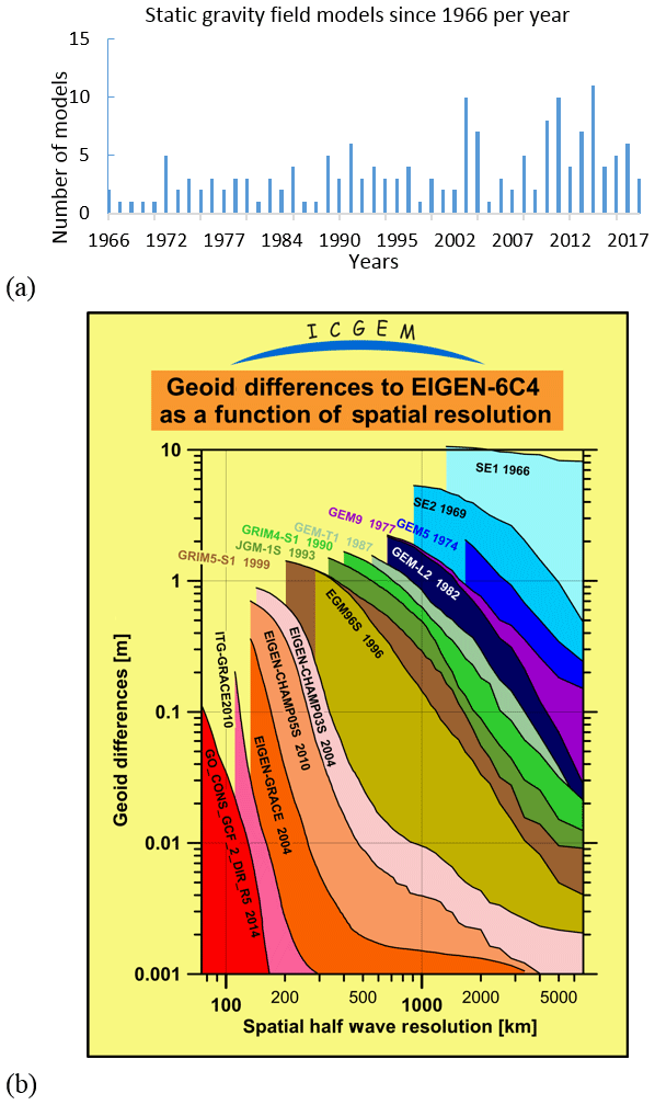
Figure 1(a) Number of static gravity field models released per year since 1966. Note the increased number of models due to the launch of the dedicated satellite gravity missions (CHAMP, GRACE, and GOCE) after 2003 and 2011. (b) The history of the improvement of the spatial resolution and the accuracy of the satellite-only gravity field models. Signal amplitude difference over the years with respect to one of the latest combined global gravity field models, EIGEN-6C4 is shown (http://icgem.gfz-potsdam.de/History.png, last access: 2 April 2019). Note that the EIGEN-6C4 is not the truth but a better approximation to the real gravity field, because it is a combination of data retrieved from satellite missions, terrestrial measurements, and altimetry-derived gravity field information. The uncertainties of the geoid signal have been reduced together with improved spatial resolution. See also the large improvement between the EGM96S and EIGEN-CHAMP03 due to the contribution of the CHAMP measurements.
By January 2019, the ICGEM service provides access to 168 static gravity field models, more than 20 temporal gravity field models (including different releases from same institutions between the years 2002 and 2016), 18 topographic gravity field models and finally models for three other celestial objects (6 for Mars, 18 for the Moon, and 2 for Venus). The ICGEM service plans to continue its long-term services with new releases of better-quality static and temporal gravity field model contributions from the recently launched GFZ and NASA mission GRACE-FO (Flechtner et al., 2014) and ongoing reprocessing efforts by GOCE (Siemes, 2018) and GRACE mission data (Dahle et al., 2018; Save et al., 2018; Yuan, 2018) as well as contributions from the New Generation Gravity Missions. Considering the number of visits to the ICGEM website during the last few years, it has become obvious that the ICGEM service is recognized as a highly demanded service by the community and used very actively worldwide. The distribution of visits of the ICGEM service by continent and the corresponding numbers between May 2018 and December 2018 are shown in Fig. 2.
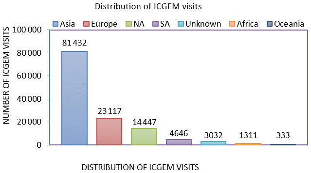
Figure 2Distribution of ICGEM visits over continents between May 2018 and December 2018. NA is for North America, SA is for South America, and unknown is for anonymous entries.
In the near future, the old G3 Browser, which showed the time variation of gravity field at any desired point or predefined basin, will be available again with improved features developed for both advanced researchers and educational purposes. A specific web interface will be made available for the user to calculate and visualize time series of mass variations. The results will again be available both in PNG and ASCII formats. Moreover, new services are among our future plans, such as the provision of time series of the changes in the gravity field of the Earth due to the flattening retrieved from SLR measurements from different institutions and agencies, the offer of the calculation of horizontal gravity gradients in the ICGEM calculation service, and development of strategies for sharing the external datasets used in the evaluation (e.g. GNSS/levelling-derived geoid undulations).
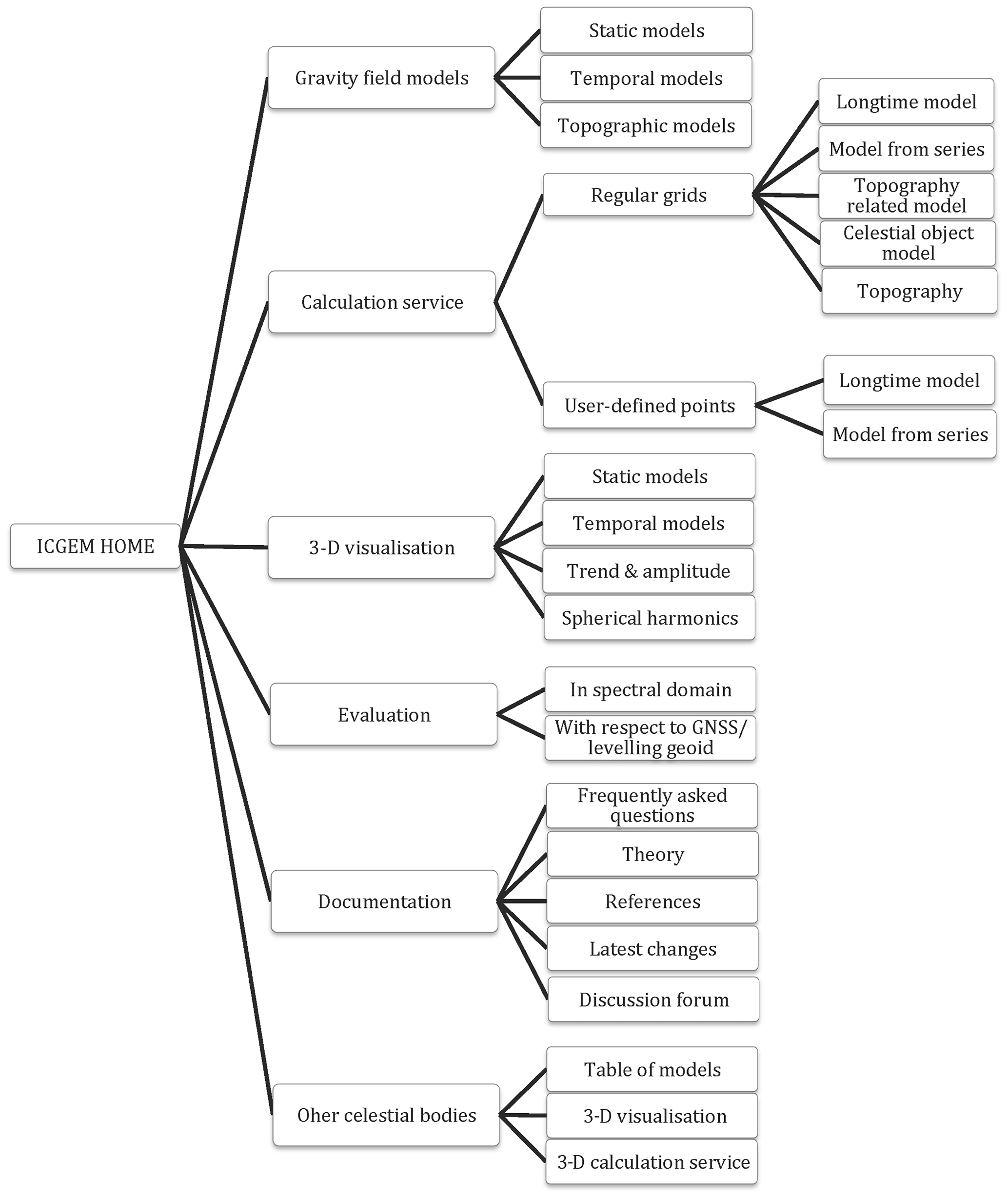
To realize the above-mentioned future plans, the development of a new modernized and more flexible ICGEM website was necessary, which was realized and made available by GFZ in May 2017 (see also Sect. 5). A scheme of the current website structure of the ICGEM service is presented in Fig. 3.
2.2 Scientific background and ICGEM's data
The global gravity field model of the Earth is a mathematical model which describes the potential of the gravity field of the Earth in the 3-dimensional space. The terms “gravity field” and “gravitational field” are commonly mixed or used interchangeably. Therefore, we will start with the basic definition of the two terms for the sake of clarity in the rest of the paper. In geodesy, there is a clear difference between the two terms. Gravitational potential, V, is formed by the summation of pure gravitational forces of the masses of the Earth, whereas gravity field potential, W, is the sum of the potential of the Earth's gravitational attraction, V, and potential of the centrifugal force due to the Earth's rotation.
Within this concept, a global model of the Earth's gravity field is a mathematical function which approximates the real gravity field potential and allows physical quantities related to the gravity field to be computed, i.e. the gravity field functionals at any position in the 3-dimensional space. A gravity field model should therefore contain both a model of the gravitational potential and a model of the centrifugal potential. Because the modelling of the centrifugal potential is well known and can be done very accurately (Hofmann-Wellenhof and Moritz, 2006), the relevant and challenging part of a gravity field model is the modelling of the gravitational field. Therefore, the term “gravity field model” is also very often used in the sense of a gravitational field model. In this article, the model coefficients are representative of the gravitational field, and the gravity field is used when the centrifugal potential is included in the computation of the gravity field functionals.
Due to mass redistribution on, inside, and outside the Earth for different reasons, the gravity field changes with respect to time. Although these temporal changes are very small and/or very slow, they can be measured (e.g. using GRACE mission data) and modelled up to a certain spatial and temporal resolution (Wahr et al., 1998, 2004; Schmidt et al., 2006). ICGEM also provides access to these temporal gravity field models.
Models approximating the real (true) gravity field can be developed based on different mathematical representations, e.g. ellipsoidal harmonics, spherical radial basis functions, or spherical harmonic wavelets, which are all harmonic outside the masses (outer Earth). In practice, solid spherical harmonics are widely used to represent the gravitational potential (or geopotential) globally, which excludes the centrifugal potential. Solid spherical harmonics are an orthogonal set of solutions to the Laplace equation, represented in a system of spherical coordinates (Heiskanen and Moritz, 1967; Hofmann-Wellenhof and Moritz, 2006).
The datasets available via the ICGEM service are the spherical harmonic coefficients, which together with the spherical harmonic functions approximate the real gravitational potential of the Earth and/or its variations. The spherical harmonic (or Stokes') coefficients represent the global structure and irregularities of the geopotential field in the spectral domain (Heiskanen and Moritz, 1967; Moritz, 1980; Hofmann-Wellenhof and Moritz, 2006; Barthelmes, 2013) and the formulation of the relationship between the spatial and spectral domains of the geopotential is expressed as follows:
where V is the gravitational potential; r,φ and λ correspond to the spherical geocentric coordinates of the computation point (radius, latitude, and longitude); R is a (mathematically arbitrary) reference radius (in geodesy usually the mean semi-major axis of Earth is used); GM is the gravitational constant times the mass of the Earth; l and m are degree and order of spherical harmonic, lmax is the maximum degree (and order) of the model expansion, are fully normalized Legendre polynomials of degree l and order m, and and are fully normalized Stokes' coefficients.
Spherical harmonics are calculated using spherical coordinates and the normalization is defined such that the average square value of the normalized harmonics integrated over the sphere is equal to unity (Heiskanen and Moritz, 1967):
The very low degree and order of spherical harmonic functions can be physically defined and easily illustrated. For example, the describes the mass of the Earth by scaling the value of GM, the whole mass of the Earth times the Newtonian constant. Therefore its value is close to 1. The degree 1 spherical harmonic coefficients, , and are related to the coordinates of the geocentre, and if the coordinate system's origin coincides with the geocentre, they are equal to zero. The coefficients and are related to the mean rotational pole position. A tutorial on the representation of the spherical harmonics is available on the ICGEM website (http://icgem.gfz-potsdam.de/vis3d/tutorial, last access: 6 May 2019) and an example of three different degree and order of spherical harmonics is shown in Fig. 4.
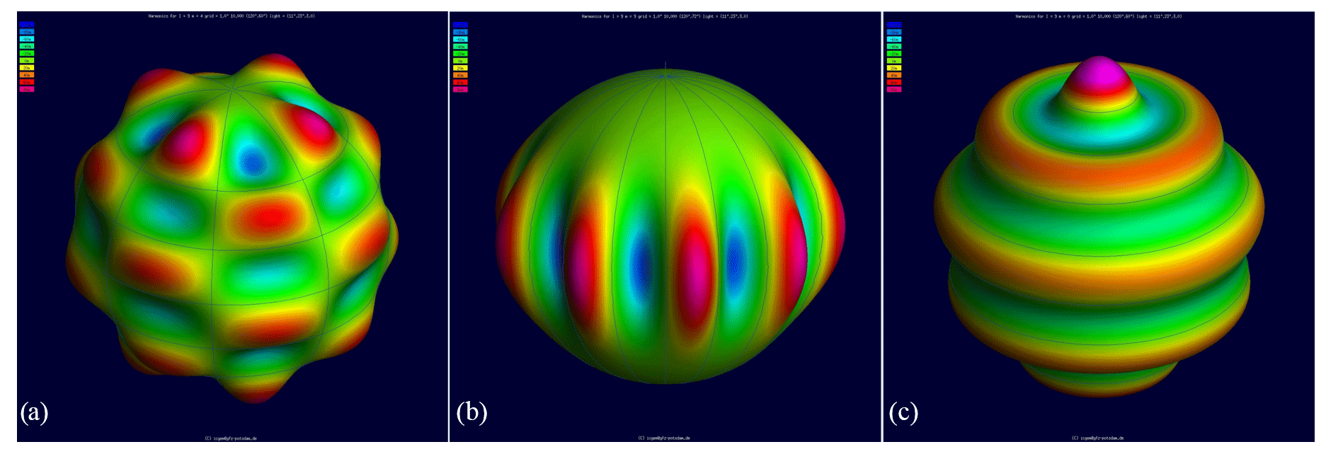
Figure 43-D visualization of spherical harmonics as a tutorial. The images show one specific surface spherical harmonic of degree l and order m such as (a) tesseral (l=9, m=4), (b) sectorial (l=9, m=9), and (c) zonal (l=9, m=0) spherical harmonics.
A mathematical representation of a gravitational field model using summation of spherical harmonics is displayed in Fig. 5. Sectorial, zonal, and tesseral spherical harmonic functions multiplied by the corresponding coefficient values are used to develop a gravitational field model of the Earth expanded up to degree l and order m. The spherical harmonic degree expansion corresponds approximately to the spatial resolution of or , where 20 000 km is the half wavelength of the equatorial length and l is the spherical harmonic degree. A spherical harmonic model of the gravitational field up to maximum degree lmax consists of coefficients (see also Fig. 5).
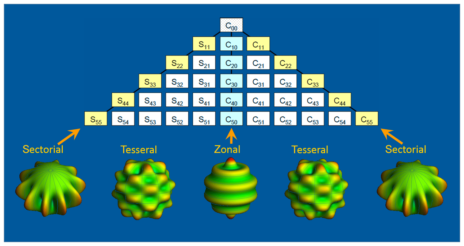
Figure 5Mathematical representation of gravitational field potential using sectorial, tesseral, and zonal spherical harmonics. A spherical approximation of the gravitational field up to a maximum degree of lmax consists of (lmax+1)2 coefficients.
The terms and and their variations are the fundamental data of the ICGEM service that are retrieved from real gravity measurements and satellite observations and derived quantities as well as forward modelling using high-resolution digital elevation models. Moreover, these coefficients are used in the calculation of the gravity field functionals directly.
At this point, it is worth mentioning the mathematically defined normal potential, which helps to approximate the real gravity potential for practical reasons. For many purposes, it is useful and sufficient to approximate the figure of the Earth by a reference ellipsoid. This is defined as the ellipsoid of revolution which fits the geoid, i.e. an equipotential surface that on average approximates the mean sea surface (i.e. in the sense of least squares fit). The normal potential together with the geometrical ellipsoid establishes the Geodetic Reference System, e.g. WGS84 or GRS80 (Moritz, 1980; Mularie, 2000). Like the gravity potential W, the normal potential U also consists of a gravitational potential and centrifugal potential. The attracting part of the normal potential can also be represented in terms of spherical harmonics. Due to the rotational symmetry, the expansion of ellipsoidal normal potential contains only the terms for m=0 and degree l= even. In most cases, the coefficients of , , , , and are used in the calculation of the normal potential, where the superscript U indicates the normal potential. Using the normal potential, the real gravity field potential can be split into two parts, the normal potential and the disturbing potential, as expressed below:
If we subtract the Stokes' coefficients (, , ..., ) of an ellipsoidal normal potential, U(r,φ), from the gravity potential, the disturbing potential, , can also be mathematically represented in terms of spherical harmonics, .
The disturbing potential is a 3-D function in space and it can be represented by the following:
The two fundamental gravity field functionals used in geosciences are very often geoid undulation and gravity disturbances, which in practice can be approximately calculated using the disturbing potential, whereas the exact calculation of gravity disturbances is possible using W and U directly. It is worth recalling that the geoid undulation is the distance between the particular equipotential surface (geoidal surface) and the surface of the reference ellipsoid (conventional ellipsoid of revolution). The gravity disturbance, on the other hand, is the difference between the magnitude of the gradient of the Earth's potential (the gravity) and the magnitude of the gradient of the normal potential (the normal gravity) at the same point (e.g. Earth's surface), .
In continental areas or over land, apart from some regions (e.g. Dead Sea area), the geoid is located inside the masses, whereas the gravity potential, W, is only harmonic outside the masses. Therefore, in order to calculate the geoid undulation from the potential W, a correction due to the masses above the geoid has to be applied, which could be done by using a representation of the topography in terms of spherical harmonics, and . Using the model spherical harmonic coefficients from potential and topography, the geoid can be expressed to a first approximation by the following:
whereas the gravity disturbance can be approximated by its radial component:
In the following section, we will give examples of different functionals and their relevant applications. For the details of the formulations of exact calculations and approximations and insight into the other functionals, the reader is referred to Barthelmes (2013).
2.2.1 Static global gravity field models of the Earth
As mentioned above, the ICGEM service was established 15 years ago to mainly collect all available static global gravity field models from different institutions under one umbrella and make these models freely available to the public. Therefore, this feature is the fundamental component of the service and special attention is paid to maintaining the complete list of static global gravity field models with a possibility of assigning the DOI number upon the model developer's request. The three main complementary data sources used to compute gravity field models are satellite-based measurements, terrestrial gravity measurements and satellite-radar-altimetry-derived quantities. The satellite-based gravity measurements cover long wavelength information of the gravity field, whereas the spatial details of the gravity field (i.e. short wavelengths or high frequencies) are collected via terrestrial, airborne and shipborne gravity measurements and radar altimetry. The altimetry records yield the sea surface height which after some corrections can be taken as mapping of the geoid over the oceans and seas (e.g. Rummel and Sanso, 1993). Consequently, a high degree and order of static gravity field models can only be developed based on a combination of the three sources which can also be supported by high-resolution topographical models. These high-resolution static gravity field models are used for regional geoid and gravity field determination in geodesy and geophysics, as well as for geodynamic interpretation and modelling; see also Table 1.
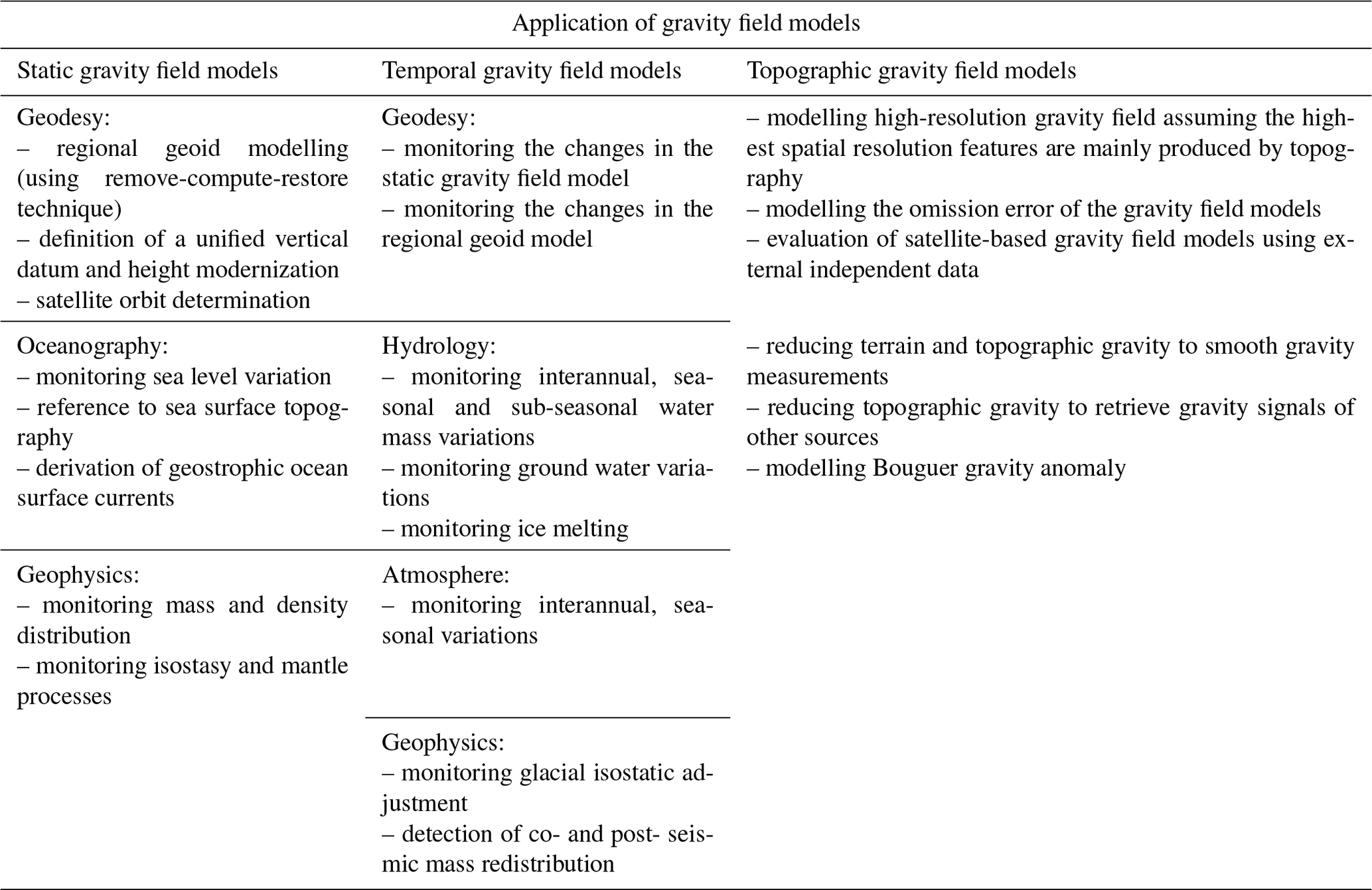
Table 1The application areas of the global gravity field models. Note that the variations refer to the mass change.
The development of the Earth Gravitational Model 2008 (EGM2008) (Pavlis et al., 2012) was a very important milestone in terms of delivering high-resolution static global gravity field models. The spherical harmonic degree and order of expansion reached up to 2190 using a combination of available gravity and topography data available worldwide. The improvement was due to the introduction of the National Geospatial-Intelligence Agency (NGA)'s worldwide terrestrial data coverage. After the release of EGM2008, different processing centres were also able to take advantage of using the EGM2008 grids for the higher-frequency components of the gravity field and to develop different “combined” high-resolution global gravity field models. As an example, one of the high-resolution static global gravity field models developed by GFZ is EIGEN-6C4 (Förste et al., 2014), which is also a combination of satellite and terrestrial data and expanded up to a spherical harmonic degree and order of 2190. EIGEN-6C4 contains data from the GOCE mission, which were not yet available for EGM2008. With the latest release of EIGEN series, the spatial resolution of the Potsdam Gravity Potato has been increased up to ∼9 km half wavelength.
The global geoid undulations and gravity disturbances computed from EIGEN-6C4 are shown in Figs. 6 and 7. Even though the Earth's interior is still a mystery, gravity can help us to understand what is inside our planet. Regions inside the Earth with higher mass densities (with respect to the mean density) produce a larger gravity attraction on the surface, whereas, on the contrary, mass deficit causes lower gravity if measured at the same point. However, if the mass densities were to change anywhere within the Earth's interior, the geoid (equipotential surface) and consequently the surface of the Earth would not stay at the same point and they would also change. As a result, the interpretation of gravity disturbances and geoid undulations (in particular globally) is more sophisticated than expected. In general, one can say that geoidal “dales” (negative geoid undulations), as in the Indian Ocean, are the result of a mass deficit in the deep mantle (Ghosh et al., 2017) and the big geoidal “bumps” (positive geoid undulations), as in the region of North Atlantic, are the result of higher mass density in the interior. In that sense, the use of gravity field models to supplement the geophysical and geological models enhances our understanding of the Earth's dynamics.
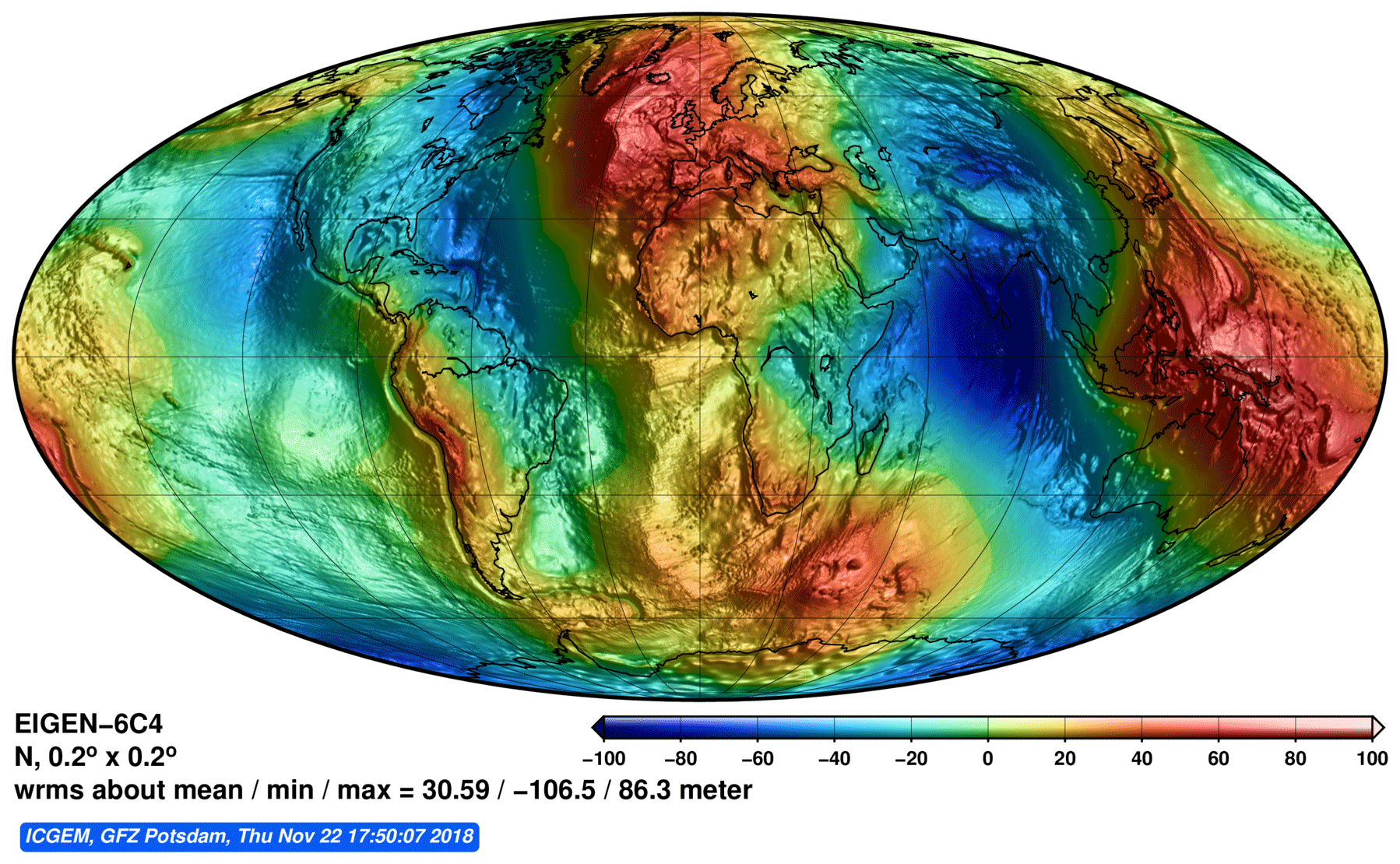
Figure 6Geoid undulation computed from the EIGEN-6C4 combined gravity field model expanded up to a degree and order of 2190.
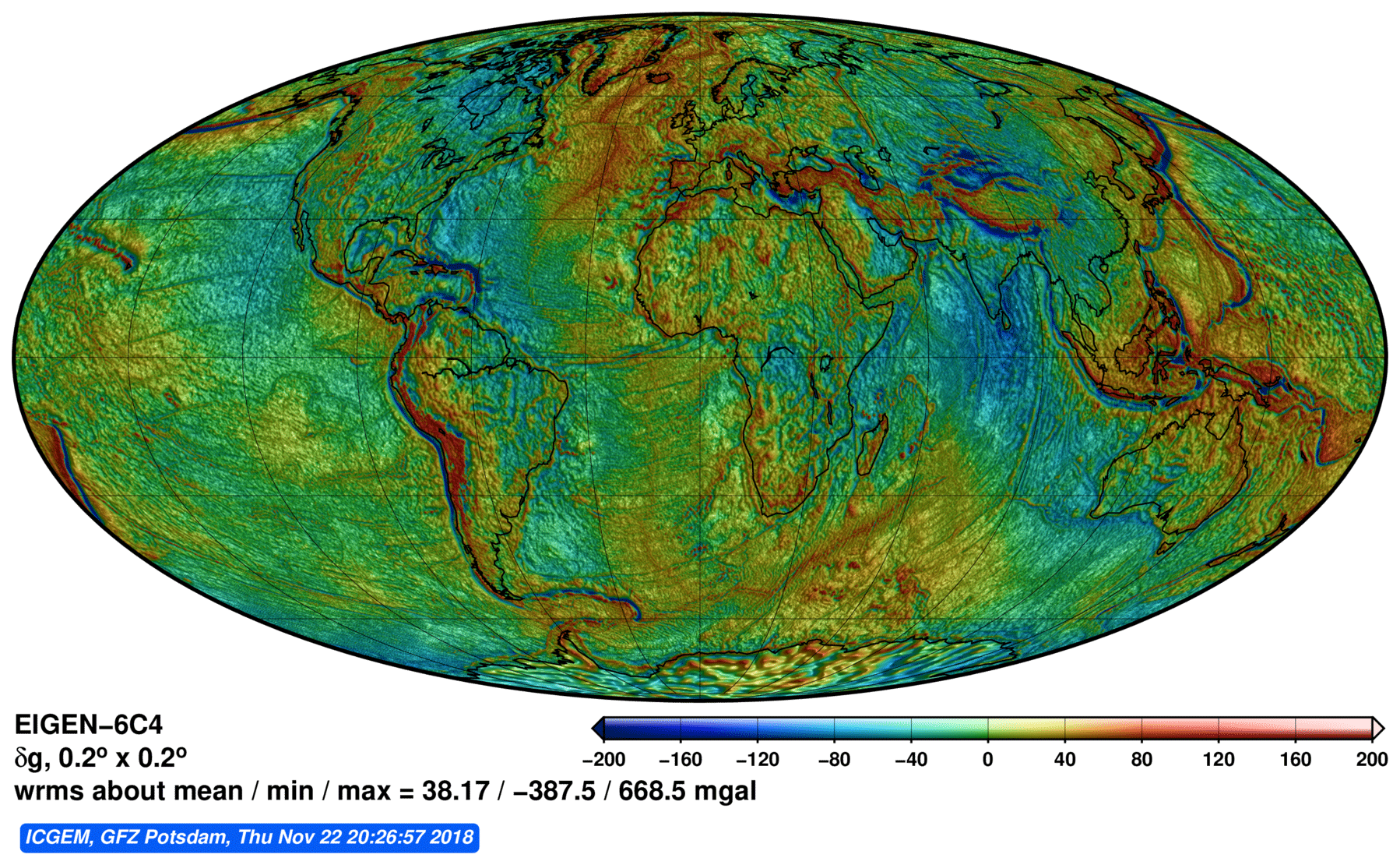
Figure 7Gravity disturbance computed on the Earth's surface from the EIGEN-6C4 combined gravity field model expanded up to a degree and order of 2190.
The studies on the development of high-resolution global gravity field continue with the reprocessed GOCE and GRACE data. Moreover, the National Geodetic Survey (NGS) has collected plenty of new terrestrial data in the USA (e.g. GRAV-D project) (Li et al., 2016) and worldwide; and it is expected that the new EGM model from NGA will be available in 2020. An experimental model, namely XGM2016, has already been released in 2016 as the precursor study for the upcoming EGM2020 with the degree and order of expansion of 719 (Pail et al., 2018). It is expected that the EGM2020 will have a spatial resolution of about 9 km or better.
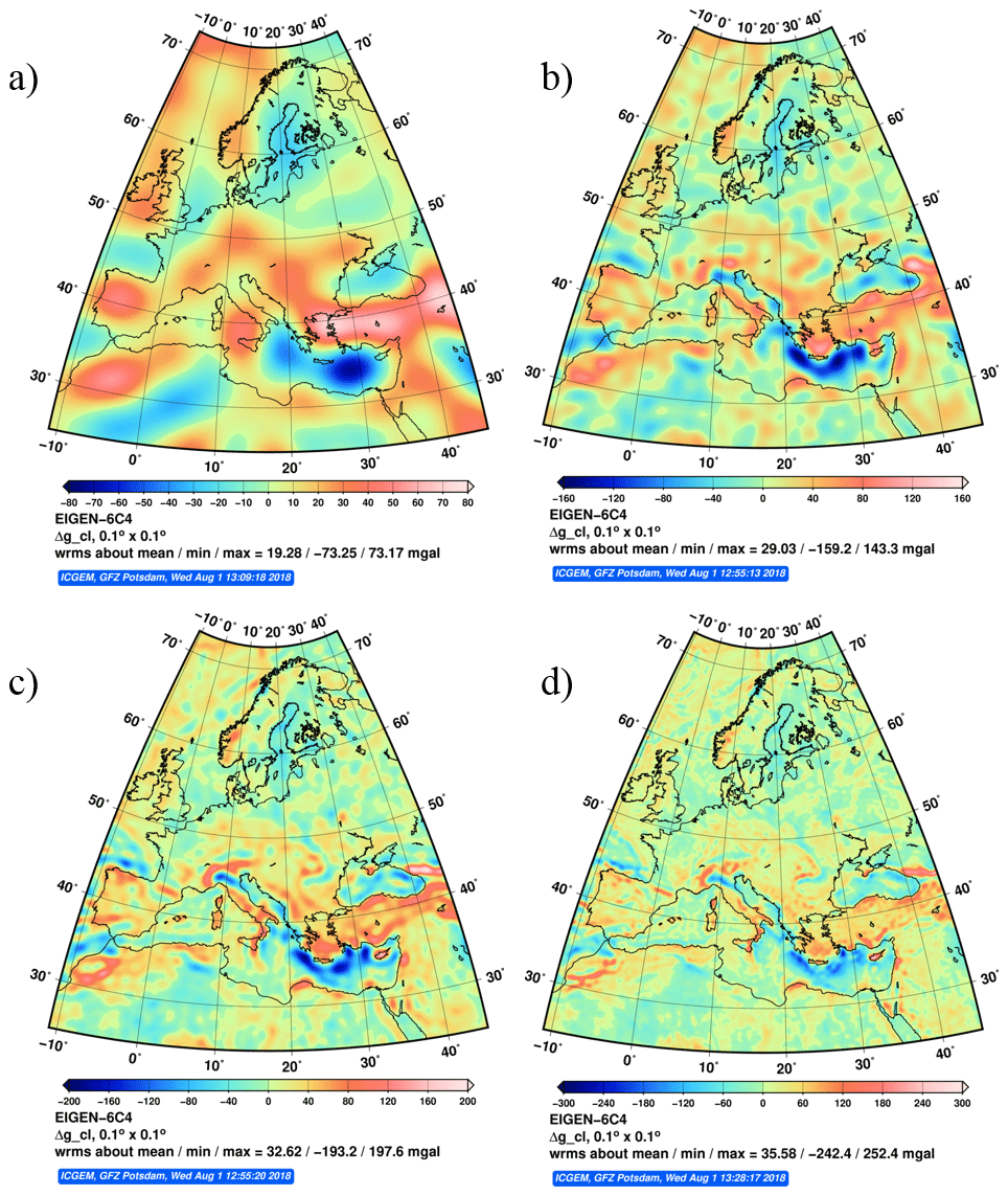
Figure 8Geographical distribution of gravity anomalies in mGal with different spectral (lmax) and spatial resolution (half wavelength λmin/2) of EIGEN-6C4. Spherical harmonic degree expansions for the four examples are as follows: (a) 50, (b) 150, (c) 250, and (d) 500 which correspond to 400, ∼133, 80, and 40 km half wavelength spatial resolutions. See the refined features and better spatial localization as the model expansion increases. For instance, topographical features such as mountains are well resolved in (d), whereas they are not precisely located in (a). The transmission borders of higher and lower anomalies in Alps and Mediterranean Sea are better resolved in (d), whereas it is not possible to distinguish and locate them precisely in (a). Note the different colour scales which have not been changed and kept as retrieved from ICGEM.
A lower-degree expansion of a gravity field model simply means a lower resolution in the spatial domain. The refined features of the gravity field are only visible using the high degree and order coefficients. Figure 8 shows four examples of different degree expansions, 50, 150, 250, and 500 of EIGEN-6C4 gravity anomalies corresponding to about 400, 133, 80, and 40 km half wavelength spatial resolution. It becomes obvious that the features are refined in the spatial domain more and more, not only over the land but also over the oceans, as the model is expanded up to higher degree and order. Accordingly, the ultimate goal would be the development of high-resolution and high-quality static gravity field model by taking advantage of different datasets available.
As mentioned in the introductory section, gravity field models are important inputs in several research fields. In geodesy, they are most commonly used for the GNSS levelling. Together with a high-quality and high-resolution geoid model, ellipsoidal heights (geometric heights) measured using GNSS sensors can provide physical heights (i.e. orthometric heights) very efficiently. In the past, the physical heights were measured via spirit levelling (or other levelling methods), which has been limited to roads and widely accessible areas only. Other application areas of static gravity field models together with temporal and topographic gravity field models are summarized in Table 1.
2.2.2 Temporal global gravity field models of the Earth
Using the models derived from input data of dedicated time periods, it is possible to monitor the temporal changes in the gravity field. The spatial coverage of the shorter period observations is not as dense as for longer periods. Therefore, the spatial resolution of temporal gravity field models (∼300 km for monthly solutions) is lower than those of the static gravity field models (∼9 km). However, contrary to the static gravity field models, a mean over a short time provides a higher resolution in the time domain (e.g. 10 d, 1 month).
Both the GRACE and now GRACE-FO missions are fundamental in observing the variation of the global gravity field. There are three official data-analysing centres for GRACE and GRACE-FO data, namely GFZ, JPL (Jet Propulsion Laboratory), and UTCSR (University of Texas Center for Space Research), which calculate temporal global gravity field models within the Science Data System missions. Even though the software packages of the three analysis centres are independent, they use the same level 1 data (raw measurements from the satellite that are converted into engineering units, level 1A) and edited and downconverted data (level 1B) as input as well as nearly identical processing standards and background models to generate the GRACE/GRACE-FO level 2 products (e.g. spherical harmonic coefficients for monthly periods). The same processing standards (Bettadpur, 2012; Dahle et al., 2012; Watkins and Yuan, 2012) mean common properties of the data processing (e.g. removing solid Earth tides or non-tidal atmospheric and oceanic effects from measurements). After the well-known effects of other geophysical phenomena (e.g. air pressure, tides) are removed, the residuals are mainly expected to represent the water mass redistributions over a certain time period and/or geophysical signals of the solid Earth, such as the mass distributions due to big earthquakes or glacial isostatic adjustment (GIA) effect. However, mathematical methods including instrument parameterizations applied in designing measurement equations or level 1B data editing and weighting vary among the three centres, and this results in slightly different model coefficients. For the visualization of the GFZ level 2 solutions and access to ready-to-use gridded level 3 data, the reader is referred to the Gravity Information Service (GravIS) platform (http://gravis.gfz-potsdam.de/home, last access: 6 May 2019).
The three data-analysing centres release unconstrained solutions, which means that no data besides GRACE measurements are applied and no regularization (sometimes called stabilization) is used in the solution. After the solutions are retrieved, the lower-degree (C20) component of the temporal gravity field from GRACE/GRACE-FO is replaced with higher-accuracy values derived from the SLR measurements. The disadvantage of these unconstrained models is the fact that the high-degree coefficients have large errors (e.g. from aliasing of tidal and non-tidal mass variations or errors in the satellite-to-satellite tracking) and they are not recommended to be used directly (i.e. without filtering). On the other hand, users are free to develop their own filters or apply the commonly used DDK filters (Kusche et al., 2009), which are also offered in the ICGEM calculation service.
Temporal gravity field models developed by different institutions and agencies can be found at http://icgem.gfz-potsdam.de/series (last access: 6 May 2019) (see also Fig. 3). Even though the initial models are derived based on the monthly coverage of GRACE observations, recently, daily models computed using state-of-art techniques are published via the ICGEM service (Mayer-Gürr et al., 2018). Moreover, combinations of different measurements from different satellites, such as SLR, CHAMP, and GRACE, are used to derive monthly solutions (Weigelt et al., 2013) and are also included in the ICGEM monthly series database.
Each temporal gravity model has different characteristics and may help to retrieve different information depending on its data content and the application area it is used for. For instance, monthly models are very useful and important in monitoring the variations in the terrestrial hydrological cycle (Schmidt et al., 2006), ice melting (Velicogna, 2009), sea level change (Cazenave et al., 2009) and help to investigate climate-change-related variations in the Earth's system (Wahr et al., 2004), whereas daily solutions have the potential to be used to monitor short-term scale variations such as flood events and they contribute to assessing natural hazards as proven with the successful outcomes of the EGSIEM project (Gouweleeuw et al., 2018). The results are generally presented in terms of equivalent water height (EWH) or water column (Wahr et al., 1998; Wahr, 2007). Some examples of the temporal gravity field models are shown in Sect. 3.
2.2.3 Topographic global gravity field models of the Earth
Topographic global gravity field models are one of the most recent products that are included in the ICGEM service. They represent the gravitational potential generated by the attraction of the Earth's topographic masses and enrich the possible applications of the geopotential models in geodesy and geophysics (Hirt and Rexer, 2015; Grombein et al., 2016; Hirt et al., 2016; Rexer et al., 2016). In contrast to the satellite-based or combined gravity field models, gravity from these models is computed based on very high-resolution digital elevation models which describe the shape of the Earth and model of mass densities inside the topography; therefore, they are not based on real gravity measurements.
This type of model is also called a synthetic gravity model or forward model. Topographic masses used in the forward modelling include not only all solid Earth topography (rock, sand, basalts, etc.) but also ocean and lake water and ice sheets. These models can help to retrieve very high-frequency components of the global gravity field, interpret and validate real gravity measurements and global gravity field models, and help to fill the gaps in which the actual gravity measurements are limited or not available, as it is the case in EGM2008 (Pavlis et al., 2012). More importantly, they can be used to subtract the topographical gravity signal from the gravity measurements and model-computed gravity data and make any other gravity signals visible that are related to the inner Earth. Therefore, use of these models is becoming more important in all kinds of geophysical applications. An example of topographic model-computed gravity anomalies in the Antarctica region together with the EGM2008 gravity anomalies in the same area is shown in Fig. 9. Note the resolved features in topographic model dV_ELL_Earth2014_plusGRS80 (Rexer et al., 2016) due to the availability of the high-resolution topography data in the area. The typical applications for using these models are given in Table 1 and a list of currently available topographic gravity field models can be found at http://icgem.gfz-potsdam.de/tom_reltopo (last access: 6 May 2019) (see also Fig. 3).

Figure 9The classical gravity anomalies which are also known as free-air gravity anomalies computed on the Earth's surface based on (a) the topographic model dV_ELL_Earth2014_plusGRS80 and (b) EGM2008 using the model's highest degree and order available, 2190. It is clearly seen that the features in Antarctica are better resolved in (a). Note that the scale is kept as it is for individual cases on purpose since the present forms of the figures are exactly what the ICGEM calculation service provides.
2.2.4 Models of other celestial bodies
Gravity field models for other celestial bodies, such as the Moon, Venus, and Mars, are byproducts of the ICGEM service. They are provided due to the interest of the model developers and users. These models have the same mathematical representation, i.e. expansion of spherical harmonic series, as the static gravity field models of the Earth. Therefore, it is convenient to also include these models in the ICGEM calculation and visualization services. These models are also developed based on similar observations of the gravity field of the body. For instance, spacecraft-to-spacecraft tracking observations from the Gravity Recovery and Interior Laboratory (GRAIL) have been used to develop the most detailed gravitational field of the Moon so far (Zuber et al., 2013).
3.1 Calculation service
By the time that the ICGEM service was established, it was naturally installed together with calculation and visualization services. Due to the interest of scientists and students worldwide, the ICGEM team has developed a web interface to calculate gravity field functionals (e.g. geoid undulation, height anomaly, gravity anomaly) from the spherical harmonic representations of the Earth's global gravity field on freely selectable grids with respect to a reference system of the user's preference. This service is the only online service worldwide available that computes a variety of gravity field functionals with the GMT plots (Wessel et al., 2013) provided for grid values and the option to download the computed values. During the 15 years, interested researchers and students have used the ICGEM service extensively for calculating gridded gravity field functionals (see Fig. 10). Calculated results are not only provided in ASCII format but also visualized using the Generic Mapping Tools (GMTs) software (Wessel and Smith, 1998; Wessel et al., 2013) with the basic statistics provided. An example can be found in Fig. 11.
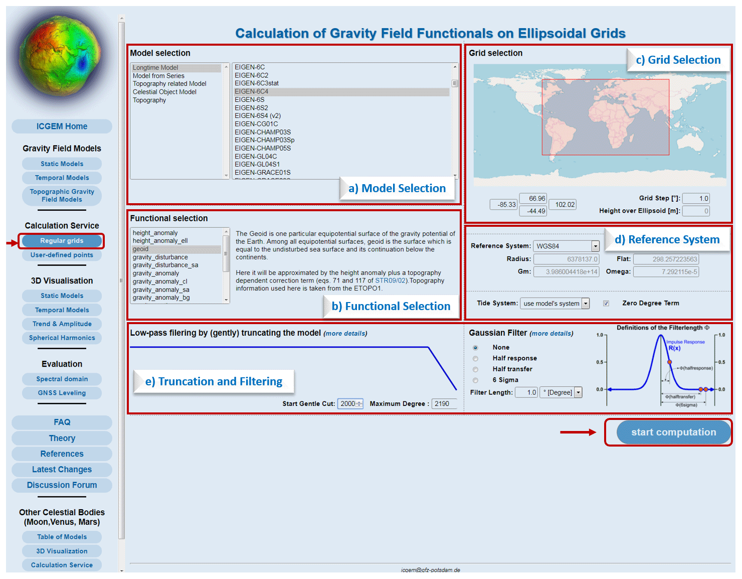
Figure 10Snapshot of the calculation service interface. The calculation settings allow the user to choose (a) the model of preference from the list of global gravity field models, (b) the functional of interest with a short definition provided and link to the equations detailed in the technical report, (c) the boundaries of the area and the grid interval, (d) the reference and tide system, and (e) the truncation degree and filtering before starting the computation. The grid area can also be selected using the red rectangle in (c) by simply changing its boundaries or entering the coordinates manually. Moreover, the grid interval can be entered in terms of degrees.
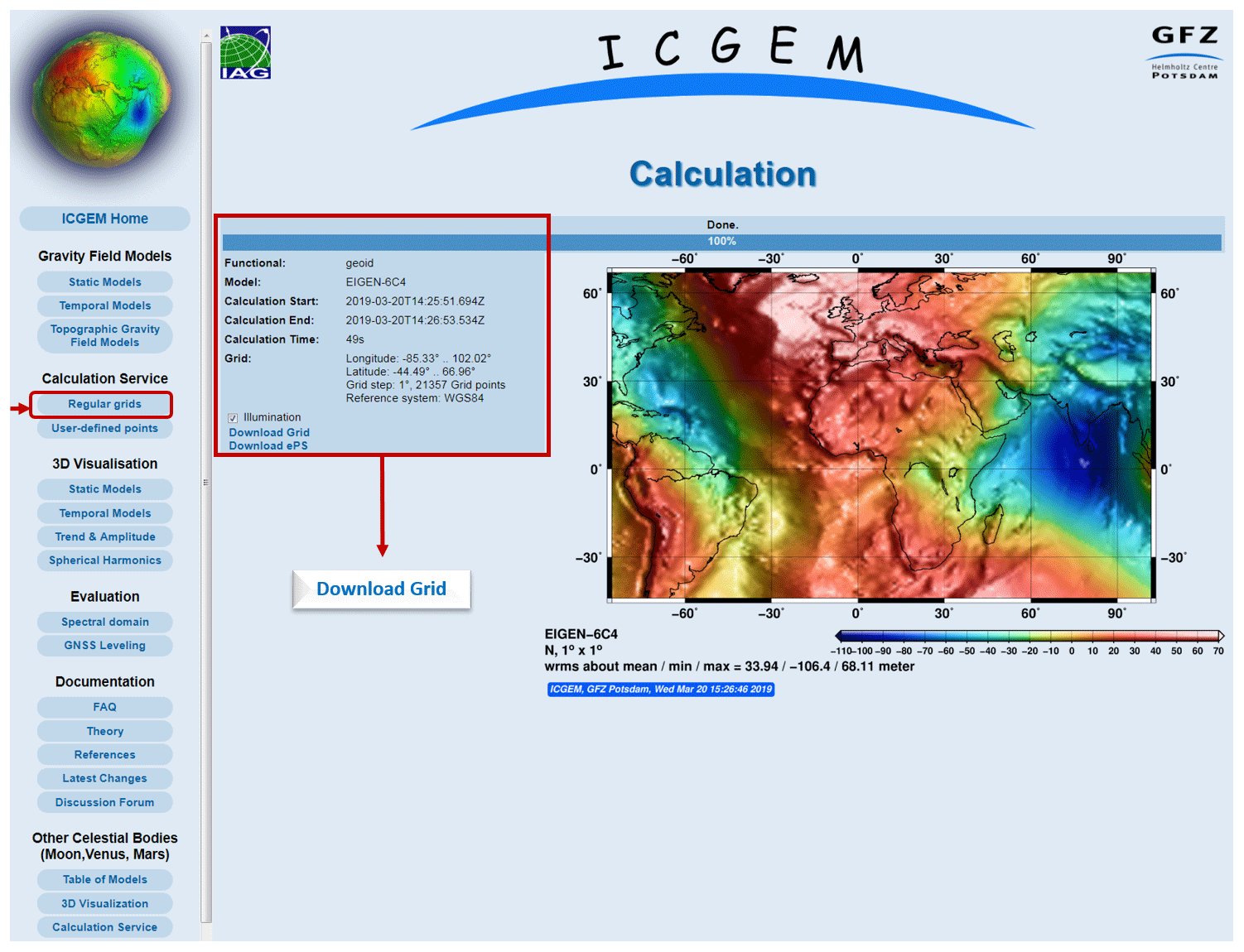
Figure 11Snapshot of the calculation service interface with the results from the input settings entered in Fig. 10, provided in numerical and map view. The figure and grid values can be downloaded from the same page and the figure can be illuminated for better visibility of the features.
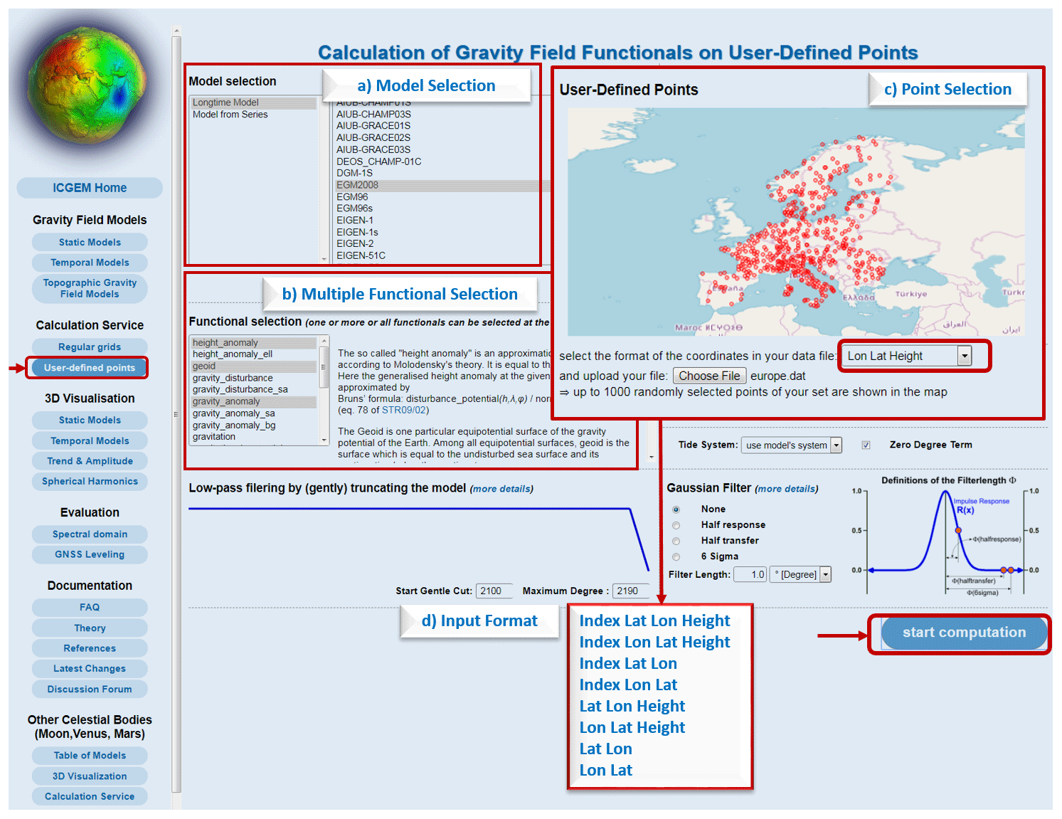
Figure 12Snapshot of the point value calculation service on ICGEM, (a) the model selection, (b) functional selection (choosing multiple functionals or all is possible), (c) input file selection and mapping of the location of user-defined points, and (d) input file format as a TXT file. The example shows the GNSS/levelling benchmark points in Europe that are also used in the ICGEM static model evaluation.
Starting from December 2018, the ICGEM service also introduced the calculation of gravity field functionals at a user-defined list of points, which was a request from the users. The list of the particular points can be prepared by the user in one of the allowed formats and the calculations are performed directly at those particular points. Different heights for different points can be introduced in the point calculation, which is different to the grid calculation where the height is assumed the same for all the grid points and consequently delivers results faster. For the point calculations, after the user uploads the text file of the set of data points in a predefined format (see Fig. 12), the points are displayed on the map. The example in Fig. 12 shows the GNSS/levelling benchmark points in Europe, which also are used in the geoid comparisons in the model evaluations.
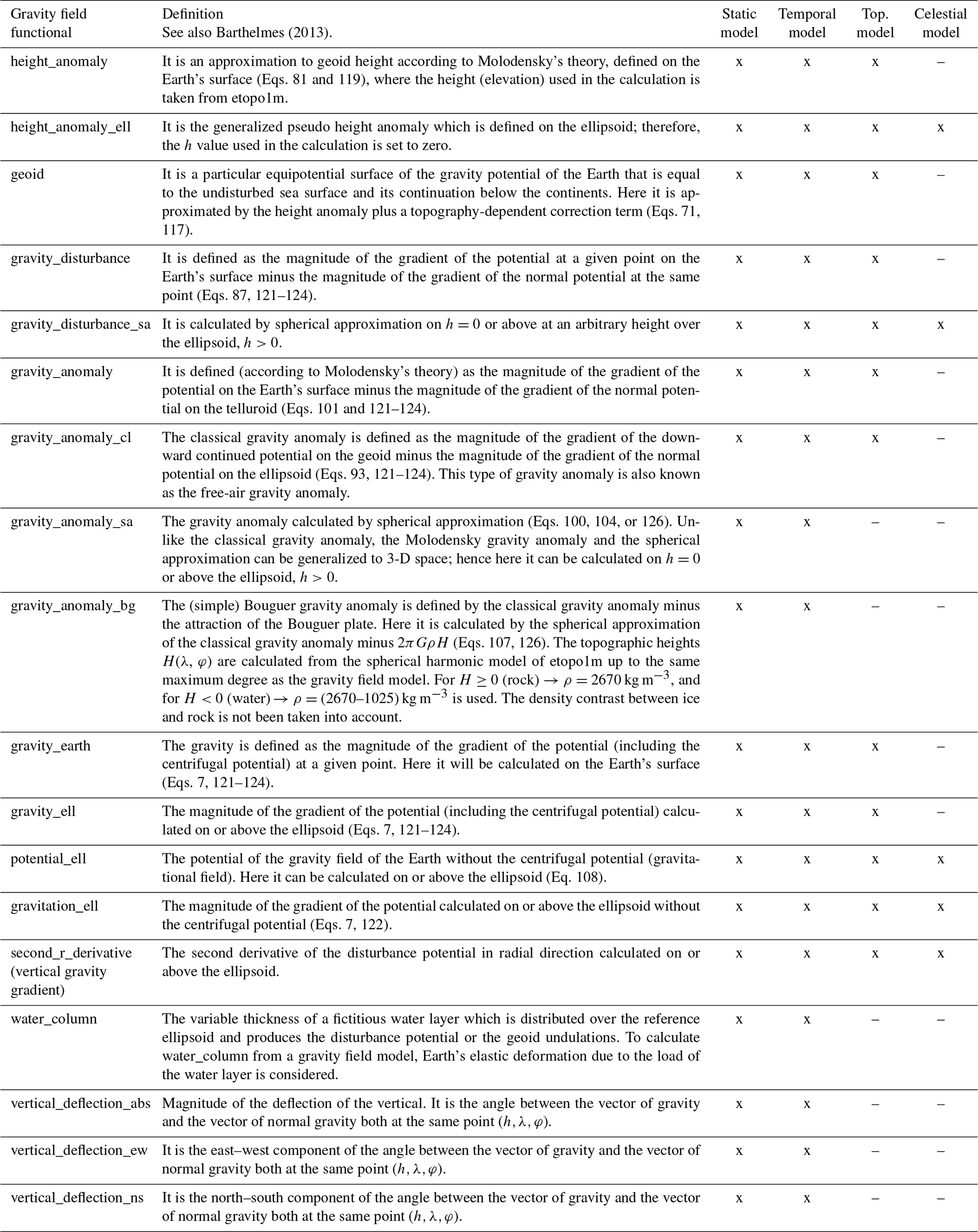
Some of the gravity field functionals are calculated based on a particular reference system in 3-D, while some others depend on the 2-D position only. Over the years, the list of functionals has also been expanded based on requests. For the 3-D functionals, the ICGEM calculation service provides different options for the reference system such as the commonly used WGS84 (World Geodetic System 1984) and GRS80 (Geodetic Reference System 1980). In addition, it provides users with the option to define their own reference system by providing the radius (semi-major axis), GM, flattening ratio (f), and angular velocity of the rotation (ω). Considering that researchers are working in different regions of the world based on different normal ellipsoid reference systems, this feature is very helpful and eliminates the time the user needs for the transformation between the reference systems. The descriptions of the gravity field functionals computed via the calculation service are given in Table 2 and the equations referred to are given in Barthelmes (2013) in detail.
Table 2The list of gravity field functionals available on the calculation service for grid and point calculations. The detailed description and definitions of the gravity field functionals are given in detail in Barthelmes (2013). The equation numbers (Eqs.) refer to the same document. Top. model is the topographic model.
Another component in the calculation of the gravity field functionals is the systematic effect that is due to the reference tide system regarding the flattening of the Earth. This is important for the definition of the geoid. Three different tide systems, namely tide-free, zero-tide, and mean-tide systems (Lemoine et al., 1998), can be selected via the given options on the calculation page. It is worth remembering the following:
-
In tide-free systems, the direct and indirect effects of the Sun and the Moon are removed.
-
In zero-tide systems, the permanent direct effects of the Sun and Moon are removed but the indirect effect related to the elastic deformation of the Earth is retained.
-
In mean-tide systems, no permanent tide effect is removed.
The geoidal surface is generally given in terms of geoid undulations or geoid heights with respect to a reference system. The reference system consists of a best-approximating geometric rotational ellipsoid (normal ellipsoid) and an associated best-approximating ellipsoidal normal potential U. The normal potential is defined in such a way that its value on the normal ellipsoid is U= constant =U0 and approximates the real value W0 as well as it is known (at the time when this reference system is defined). Hence, the reference system also defines the value W0=U0. It is worth noting that an improvement of the numerical estimation of W0 value is still under discussion and requires up-to-date information of small changes in gravity field potential (e.g. due to sea level rise).
Following the above discussion, the zero-degree term arises when W0 is chosen or calculated differently to U0 and/or when GM values between the geopotential model and reference ellipsoid are different. Therefore, this term needs to be taken into account to calculate the geoid undulation correctly with respect to a known reference ellipsoidal surface (see also questions 16, 17, and 18 in http://icgem.gfz-potsdam.de/icgem_faq.pdf, last access: 6 May 2019).
3.2 3-D visualization service
An online interactive visualization service of the static gravity field models (geoid undulations and gravity anomalies), temporal models (geoid undulation and equivalent water column), trend and annual amplitude of GRACE gravity time variations, and spherical harmonics as an illuminated projection on a freely rotatable sphere are available on the ICGEM service. The visualization service was established to provide the users with a sophisticated visual representation of the gravity-field-related products and it was the first of its kind when it was available to the general public as Potsdam Gravity Potato. It has become a service which is very useful for quick-look analyses of the functionals globally and also for tutorial purposes of different educational levels (http://icgem.gfz-potsdam.de/vis3d/longtime, last access: 6 May 2019). Users of this service can select the functional, the model, the grid interval, and the spherical harmonic degree expansion of the model to see the results on the 3-D visualization. Moreover, the rotation tool can be used to locate different regions of the globe and the selected image can be exported via the export tool. An example of geoid undulation and gravity anomalies is shown in Fig. 13.
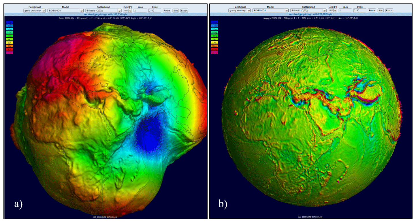
Figure 13Examples of the visualization service for (a) geoid undulation and (b) gravity anomaly computed from a high-resolution combined static gravity field model.
Static model visualization also enables the demonstration of the differences between two models with a selected grid interval and spherical harmonic degree expansion. Zoom functions are available, which also makes this tool very useful for advanced users who want to investigate particular regions of interest based on different models. Using the 3-D visualization service, as an example, the substantial differences between the new experimental geopotential model XGM2016 of the upcoming Earth Gravitational Model 2020 (EGM2020) and the older EGM2008 model are displayed for the Antarctica and Himalaya regions (Fig. 14). As shown in Fig. 14a, the differences are mostly due to the “terrestrial” update in Antarctica, which is due to the updates of the “non-data” or “synthetic” values used in the EGM2008. Similar differences are also shown for the Himalaya regions in Fig. 14b.
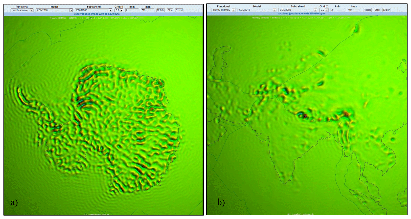
Figure 14Examples of the visualization service for the gravity anomaly differences computed from XGM2016 and EGM2018 up to a degree and order of 719 for the (a) Antarctica and (b) Himalaya regions. The EGM2008 relied exclusively on ITG-Grace03s (Mayer-Gürr, 2007) expanded up to d/o 120 to fill Antarctica with synthetic values, whereas, in XGM2016 (Pail et al., 2018), these synthetic values were derived from GOCO05s (Mayer-Gürr et al., 2015) and from forward modelling of ice and rock thicknesses from the Earth2014 digital terrain model (Hirt and Rexer, 2015).
3-D visualization of temporal gravity field models displays the computation of geoid undulation and equivalent water height (EWH) from different daily and monthly series with an option of using filtered or unfiltered model coefficients. The visualization tool can also be used for animation purposes for different monthly series. Two different monthly series, January 2009 and May 2009, filtered using DDK1 filter are displayed in Fig. 15a and b. The differences between the two figures represent the mass changes. The visualization of the trend and annual amplitude of GRACE measurements that are collected between 2002 and 2015 are also available as shown in Fig. 15c and d, respectively. Clearly visible in these representations is the ice melting trend over Greenland and Alaska, the GIA effect in the Hudson Bay area, and the annual mass variation in the Amazon region, which have been some of the priority research topics during the last few years.
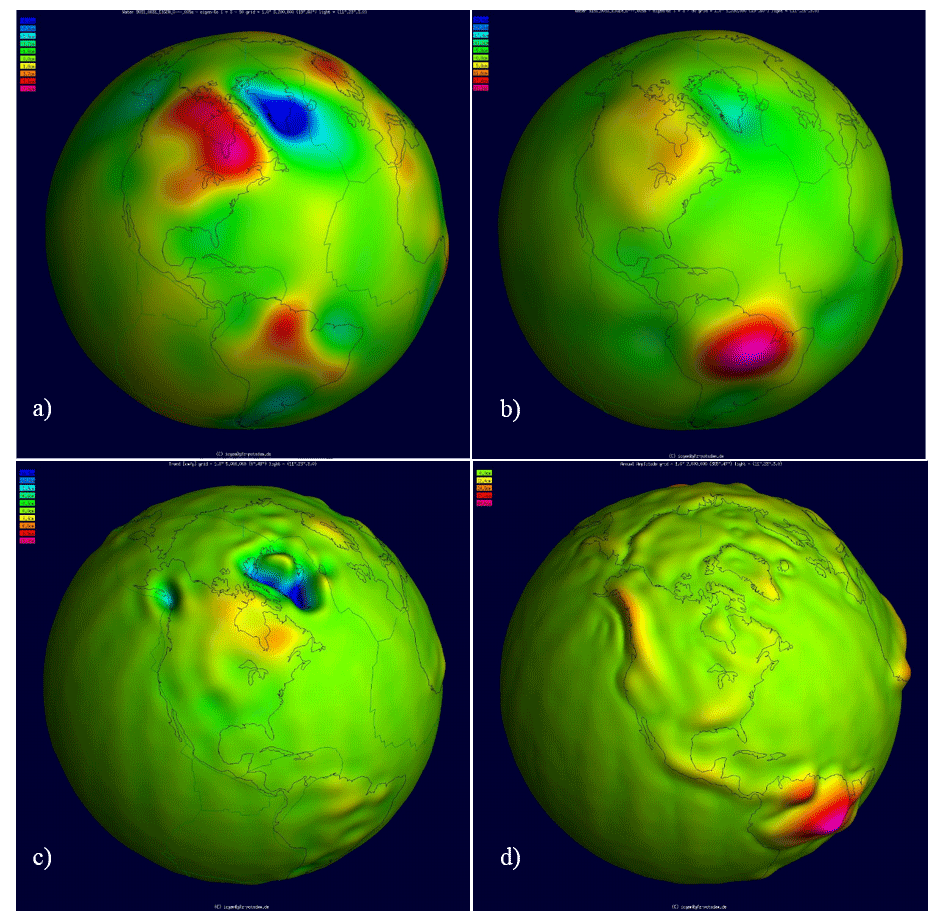
Figure 15Snapshot of visualization service for temporal models (a) EWH in January 2009 and (b) EWH in May 2009. Note that the EWH difference between the 2 months represents the mass change trend (c). Note the strong effect due to the GIA in the Hudson Bay area, Canada, and ice melting in Greenland and Alaska. (d) Annual amplitude, where the large signal amplitude in the Amazon region is noticeable.
3.3 Evaluation of global gravity field models
With its additional evaluation service, ICGEM goes beyond the collection and distribution of the gravity field models. Before being published as part of the ICGEM service, each new global model is investigated to ensure that its content is worthy of being published in the service. There are two techniques covered in the ICGEM evaluation procedure: (1) comparisons with respect to other (already identified as reliable) global models in the spectral domain using signal degree amplitudes, (2) comparison of the model-calculated geoid undulations with respect to a set of GNSS/levelling-derived geoid undulations for different regions of the Earth.
3.3.1 Model evaluation with respect to other models in the spectral domain
One of the most commonly used techniques in the assessment of global gravity field models is looking at the cumulative signal and noise amplitudes per degree and signal and noise amplitudes. The signal can be computed using the spherical harmonic coefficients, whereas the noise can be computed using the associated errors. In the ICGEM evaluation procedure, we use the signal degree amplitudes, σl of the functional of the disturbing potential at the Earth's surface but not the error degree amplitude, since not all of the models include the same type of error. Some of the models include formal errors, whereas other ones include calibrated errors. The signal degree amplitudes of the models can be computed by
in terms of unitless coefficients. The outcomes refer to the internal accuracy of the global model in terms of geoid height, gravity anomaly, or other functionals. The error degree variance can also be computed using the spherical-harmonics-associated error coefficients using the same formula (Eq. 7). The outcomes of this analysis do not necessarily represent the model characteristics or signal-to-noise ratio of a particular area or a region but represent the model characteristics globally. In our comparisons, we use geoid heights signal amplitudes per degree in particular, which can be computed via
in terms of metre. An example of the comparison of two recent static global gravity field models, the satellite-only model GOCO05S (Mayer-Gürr et al., 2015) and the combined model EIGEN-6C4 (Förste et al., 2014) is shown in Fig. 16.
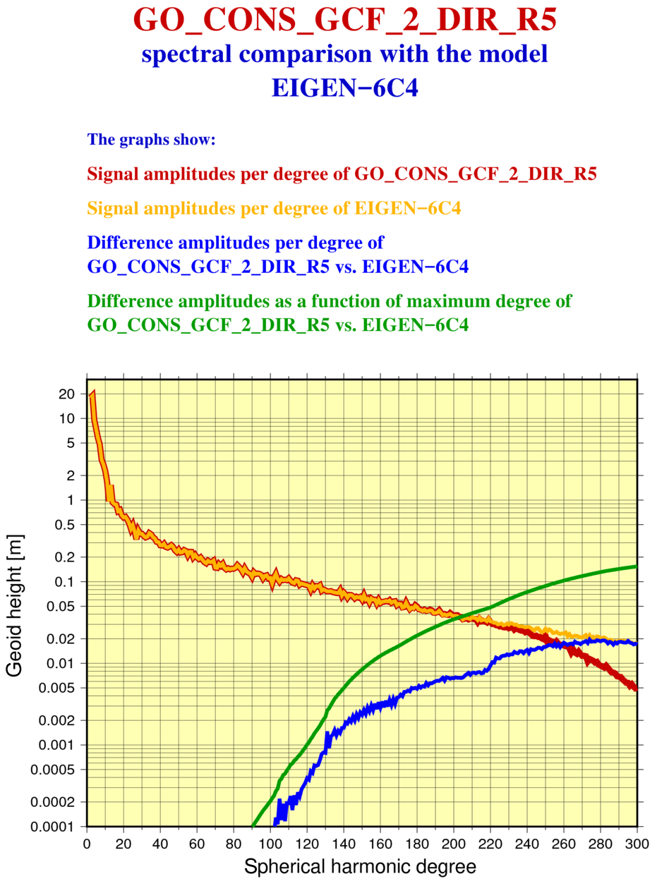
Figure 16Spectral comparison of two static global gravity field models, GOCO05S and EIGEN-6C4. Note that the comparisons are performed for each degree separately. GOCO05S is a satellite-only model, whereas the EIGEN6C4 is a combined model that uses both the satellite and terrestrial measurements. The blue curve represents the difference in the amplitude of the GOCO05S and EIGEN-6C4 combined static gravity field models per degree, whereas the green line represents the cumulative difference amplitudes of the two models as a function of maximum degree. Note the increasing difference as the degree increases due to the contribution of the terrestrial gravity data to EIGEN-6C4.
3.3.2 Model evaluation with respect to GNSS/levelling-derived geoid undulations
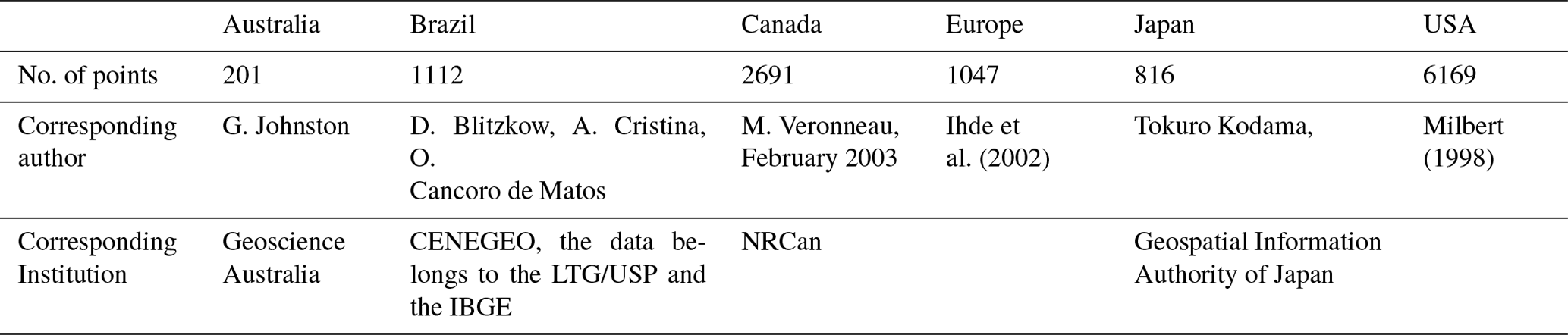
Another way of assessing a global gravity field model is to compare the model outputs with respect to independent external sources. For instance, it is very common to compare the model-computed geoid undulations with GNSS/levelling-derived geoid undulations (Gruber, 2009; Gruber et al., 2011; Huang and Véronnaeu, 2015; Ince et al., 2012; Kotsakis et al., 2009). Traditionally, geoid undulations have been derived from the ellipsoidal and orthometric heights that are measured using GNSS sensors and via levelling which is limited to the levelling benchmark points. This kind of evaluation is also valid for other gravity field functionals, such as gravity anomalies or deflections of vertical, where the model-computed values are compared with the terrestrial measurements. The advantage of this method is that it is suitable for assessing the model outcomes at a regional level or in a particular area but the assessments are only as good as the quality of the external datasets used in the validation. ICGEM has collected some series of GNSS/levelling datasets from different countries. These countries are Australia, Brazil, Canada, Japan, and the USA. Moreover, a series of data points from Europe is also included in the comparisons. More information on the GNSS/levelling data points is provided in Table 3.
Table 3Information on the GNSS/levelling benchmark points ICGEM collected during the years and corresponding authors/institutions.
CENEGEO: Centro de Estudos de Geodesia. IBGE: Brazilian Institute
of Geography and Statistics. LTG/ USP: Laboratory of Topography and
Geodesy/University of Sao Paulo.
NRCan: Natural Resources Canada.
In contrast to the global gravity field models, these data are not freely available. Their availability is limited due to the legal restrictions or the observers' own interest. Due to the relevance of these external datasets for the model evaluation, ICGEM will address this issue and develop strategies in improving the availability of these data for the general public and for the benefit of the global community.
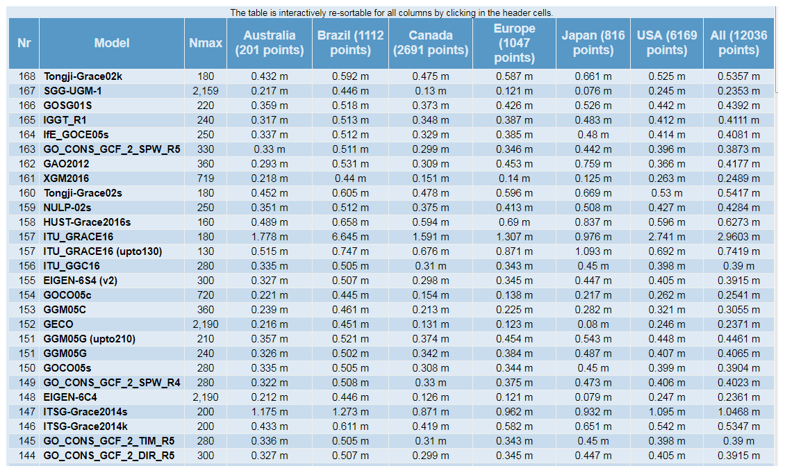
Figure 17Root mean squares of the mean differences between the model-computed geoid undulations and the GNSS/levelling-derived geoid undulations. The comparison results are shown for the most recent models and retrieved from http://icgem.gfz-potsdam.de/tom_gpslev (last access: 17 April 2019). Note that the comparisons should be realized among different type of models, e.g. combined models up to similar degrees or satellite-only models up to similar degrees. One can change the order of the models using the Nmax column.
In general, the GNSS/levelling measurements are collected over decades. Besides the epoch differences among the measurements, different GNSS or GPS equipment are used and different length of observations, and observing procedures are followed which cause the estimation accuracy of the ellipsoidal heights (h) to vary. The GNSS/levelling-derived geoid undulations can be computed via
The simple comparison of such data with model-computed geoid undulations is erroneous. These errors are not taken into account in our assessments and obviously the comparison results will only be as good as the quality of the resources, global gravity field model, and GNSS/levelling-derived geoid undulations. In principle, this evaluation is much more sophisticated than what is currently covered by the ICGEM service (Gruber, 2009; Gruber et al., 2011; Ince et al., 2012). The GNSS/levelling-derived geoid undulations should also be reduced to the same spectral content of the gravimetric geoids, which is not taken into account in our quick-check assessments since the aim of this procedure is to provide relative comparisons among the models with respect to the same set of GNSS/levelling data. Comparison results are given in the evaluation section of the service and results for the recent models are shown in Fig. 17. Interested scientists are invited to share their GNSS/levelling datasets with ICGEM to improve and extend the evaluation procedure.
3.4 DOI service
For more than a decade, the need for and value of open data have been expressed in major science society position statements, foundation initiatives, and in statements and directives from governments and funding agencies worldwide. The citable data publication with assigned digital object identifiers (DOIs) can be regarded as best practice for addressing these requirements. Ideally, the data are technically described and provided with standardized metadata, including the licence for reuse, which is readable for humans and machines. Today, datasets with assigned DOIs are fully citable research products that can and should be included in reference lists of research articles (Data Citation Synthesis Group 2014; Hanson et al., 2015).
Following the bottom-up structure of ICGEM, the DOI service was developed as a request by the user community. Global gravity field models are often shared through ICGEM months or even years before they are described in scientific research articles. The publication of static and temporal models with a DOI makes them citable and provides credit to the originators already with their publication via the ICGEM service. The DOI service of ICGEM was developed in cooperation with GFZ Data Services, the domain repository for the geosciences hosted by GFZ (http://dataservices.gfz-potsdam.de/, last access: 6 May 2019). To reduce the heterogeneity in the data documentation for static global gravity field models, standardized metadata templates for describing the models were developed that include cross-references between the model data and research articles, data reports with detailed model description and other text or data publications (see Fig. 18). At the moment, all models with assigned DOIs are published under the Creative Commons Attribution 4.0 International Licence (CC BY 4.0).
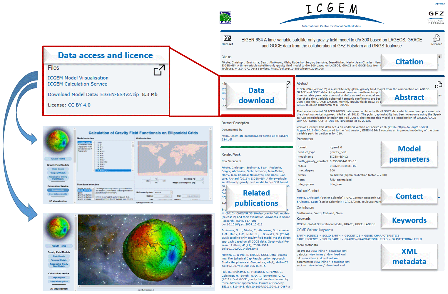
Figure 18Example and features of an ICGEM DOI landing page (EIGEN-6S4, http://doi.org/10.5880/icgem.2016.008). The DOI landing page to the right is the visualization of the metadata for data discovery that is collected for the DOI assignment. In addition to the links to the data, it includes the citation information, a data description (abstract), a table of model parameters, contact information, keywords, and links to related publications. The metadata are also provided in machine-readable XML format. The key elements of the DOI metadata are also included in the header of the data files (model coefficients). The left part of the figure is a close-up of the data download section. GFZ Data Services store a copy of the model data and provide direct links to the ICGEM visualization and calculation services with the preselection of the actual model.
For DOI-referenced models, data access is provided via specific, ICGEM branded, DOI landing pages (see Fig. 18) at GFZ Data Services and via the ICGEM website (see Fig. 19). In addition direct links to the ICGEM visualization and calculation services for the specific model are provided in the DOI landing pages. The citation of the model and the licence is also included in the header of the data files themselves.
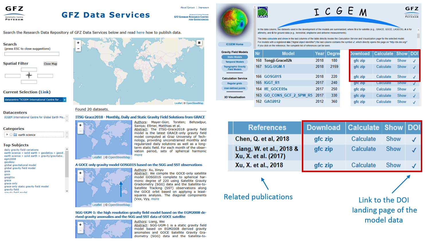
Figure 19Illustration of the two different possibilities to access the DOI-referenced ICGEM models: via the catalogue of GFZ Data Services (left) and the ICGEM website (right). GFZ Data Services have created a specific data centre for the ICGEM service (http://dataservices.gfz-potsdam.de/portal/?fq=datacentrefacet:-DOIDB.ICGEM-ICGEMInternationalCentreforGlobalEarthModels, last access: 6 May 2019). On the ICGEM website (to the right, table of models), each ICGEM model with assigned DOI is linked to the DOI landing page via the mark in the DOI column.
Since its implementation in late 2015, we have assigned DOIs to 17 static and 3 temporal series, mostly timely related to their first publication via ICGEM. As DOI-referenced datasets are required to remain unchanged, for the case of one model update we have developed a DOI versioning service with direct links between the two versions and a version history explaining the differences (e.g. Förste et al., 2016a, b). GFZ Data Services provide their DOI landing pages and metadata for each dataset in machine-readable form (schema.org and XML, respectively), following DataCite 4.0 and ISO19115 metadata standards. Metadata can be harvested via an Application Programming Interface (OAI-PMH). As a result, metadata from ICGEM models are also findable in the catalogues of DataCite (http://search.datacite.org/, last access: 6 May 2019), B2Find (http://b2find.eudat.eu/, last access: 6 May 2019) and the newly released Google Dataset Search engine (https://toolbox.google.com/datasetsearch, last access: 6 May 2019).
The documentation section of the ICGEM service consists of five subsections: frequently asked questions, theory, references, latest changes, and discussion forum. The ICGEM team responds to users' questions as soon as possible in the discussion forum. During the last few years, there were common questions from advanced users, researchers, and students that are fundamental to answer thorough analyses in different application areas. The ICGEM team has collected frequently asked questions (FAQs) and provided this collection with answers as a PDF document. The questions are answered to meet the needs of both users from different scientific disciplines and experts in the field of physical geodesy. The FAQ list is regularly updated when new questions accumulate. The last version of the FAQs can be accessed via http://icgem.gfz-potsdam.de/faq (last access: 6 May 2019).
Although the theory of the global gravity field modelling and the calculations of gravity field functionals are not presented in this paper, it is most fundamental to the development of the ICGEM service and a detailed documentation is reported in Barthelmes (2013). This scientific technical report includes the potential theory and approximations that are used in the global gravity field modelling.
ICGEM does not only collect gravitational models but also pays attention to the full documentation of the models. New model releases, new documentation, and conference and symposium presentations can be found on the ICGEM home page and in the list of latest changes. Moreover, for the convenience of the users, all relevant sources are listed in the references. This will ensure that the service and its components are available at the same place.
Moreover, the ICGEM service provides a gravity field discussion forum (http://icgem.gfz-potsdam.de/guestbook, last access: 6 May 2019), which provides users with a platform to communicate with the ICGEM team and other scientists working on similar topics. Apart from fulfilling the requirements of the service, this platform has also been used as a tool for educational purposes in which undergraduate or graduate students communicate with the ICGEM team directly. Since the interaction between the users and ICGEM team members has evolved and included extensive communications including emails, the definition of the old “guest book” was redefined and has been modified in the forum in 2016, which better represents the current status of the platform.
The new version of the forum should give the users the opportunity to discuss any topic related to the gravity field among themselves or answer each other's questions and probably share data in the future. In the following years, we will establish subsections for different topics and expand the discussion forum to be unique in this field. Without registering, anyone should be able to write comments in the forum, which will be publicly available after approval of the ICGEM team.
The original ICGEM website was established in 2003 and was based on plain HTML, Java applets, and Perl scripts. In 2016 and 2017, several components of the website received an upgrade. The web pages are generated with the Python-based framework CherryPy and Jinja2 templates. A MongoDB serves as the database backend (see Fig. 20 for an overview of the web programming scheme). In addition, the 3-D visualization received minor changes and the user interface of the calculation service has been redesigned. The programmes used in the calculation provide identical results and make use of the database to display the status of individual calculations.
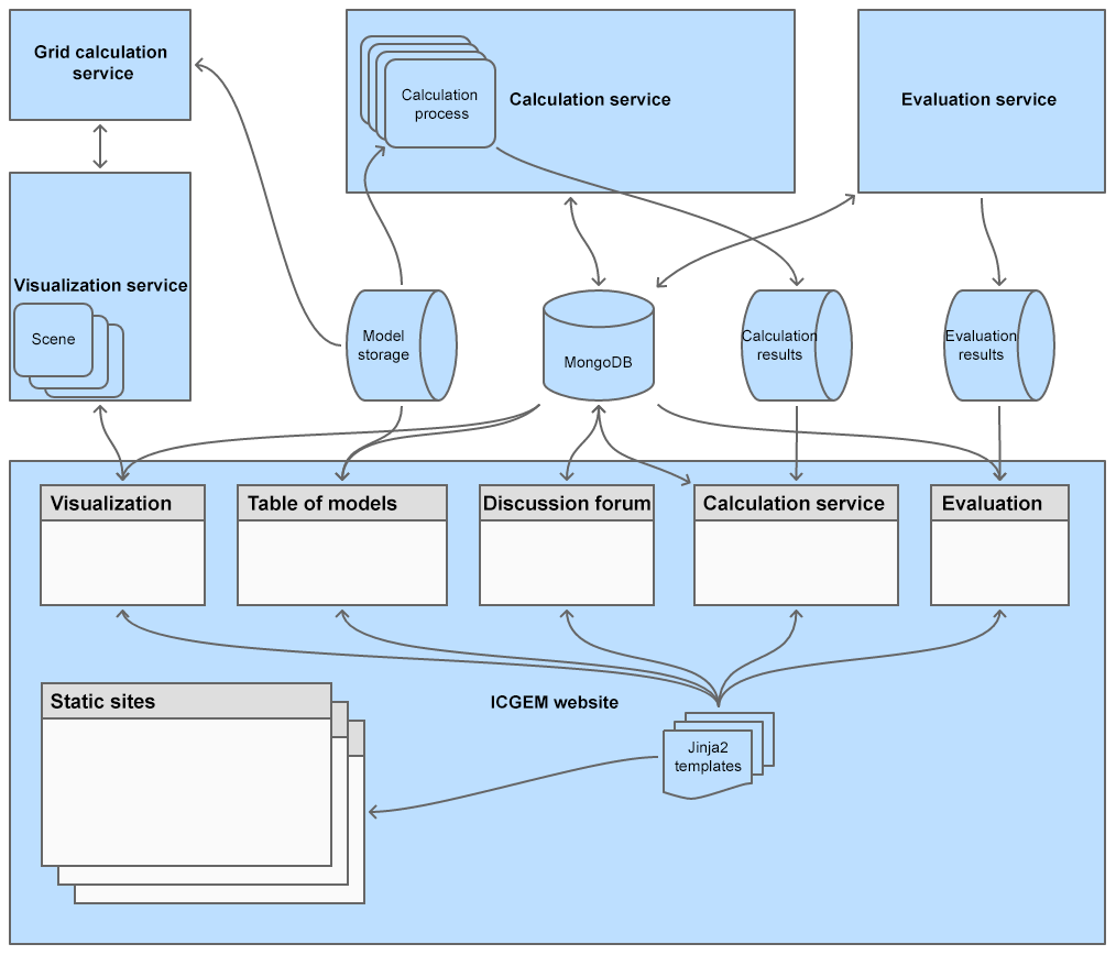
Figure 20Illustration of the scheme of the ICGEM website in terms of its web programming. Arrows indicate the direction of data flows. Cylinders are the default symbol for databases and sideway cylinders are used for file-based data storage. Model storage is file based, while the calculation results are the calculated grid files and the images converted from them. Evaluation results are only the generated images on the spectral domain page; the values in the GNSS/levelling page derive from the MongoDB. At the bottom of the scheme, every grey-white rectangle represents a subpage on the website. Similar pages, like the different visualization pages or the tables of models, are presented together, and we included only the static pages that are more interesting from a technical perspective.
Visualization service. The visualization service received minor updates primarily to ease the maintenance. Information on all models is kept in the MongoDB database. To visualize a specific model in a user's browser, the ICGEM server creates a scene, dynamically applies changes to this scene, and returns the resulting picture for display. Changes to the scene could be the rotation of the visualized model or changes of parameters.
Table(s) of models. This page simply requests all the model information from the MongoDB and displays it in a table. If a user wants to download a model, the model file is requested from the model storage.
Discussion forum. Posts from users are saved in the MongoDB and those approved by the ICGEM team are displayed on the page.
Calculation service (browser). When the user clicks on “start calculation”, the browser sends the calculation settings to the server. The calculation settings are stored in the MongoDB database and the user is redirected to the calculation status page. The calculation progress is periodically updated from the MongoDB database. When the calculation is done, the results are displayed and download links are shown.
Calculation service. The calculation service is a dedicated programme on the server that requests new calculations from the MongoDB. For new calculations a calculation process is started and progress is stored in the MongoDB to be requested by the calculation status page. After the calculation is done, the resulting grid is converted to an image. The number of concurrent calculation processes is limited, so a new calculation will have to wait until a slot is free.
Evaluation (browser). For each model, the GNSS/levelling information is saved in the MongoDB. For the spectral domain evaluation, additionally, the images of the evaluation results are loaded and displayed.
Evaluation service. In the MongoDB one model is selected as the reference model, while all other models have an attribute indicating which model was used for the evaluation. The evaluation service runs in regular intervals and requests the evaluation status of all models from the database. Models which were not evaluated with the current reference model will be automatically re-evaluated. When a new model is added, it will automatically be evaluated within some minutes. If the reference model changes, all models will be reevaluated.
Static sites. The static sites like the FAQ and theory are only Jinja2 templates and do not need any information from the MongoDB.
The overall architecture of the ICGEM website and its services is visualized in Fig. 20. The pivotal component is the MongoDB database. On the one hand, this database is used to feed forms with information about models or discussion posts and to link to file storages, and on the other hand, the MongoDB database decouples most of the server components from the user's internet browser. Therefore, long-lasting model calculations can be bookmarked for later inspection of the results. Because of its dynamic behaviour, the visualization service requires a direct communication with the user's internet browser and the MongoDB database is not used to exchange information.
The website of ICGEM with all model data, documentation, and services as described in this article is available via http://icgem.gfz-potsdam.de/ (last access: 6 May 2019). In addition, all gravity models with assigned DOIs are also accessible via the GFZ Data Services catalogue http://dataservices.gfz-potsdam.de/portal/?fq=datacentrefacet:-DOIDB.ICGEM-ICGEMInternationalCentreforGlobalEarthModels, last access: 6 May 2019). As the purpose of this article is the description of the ICGEM service with all its features, including the DOI service, we do not provide an additional DOI to all model data but refer the users to directly access the data via the ICGEM website or GFZ Data Services.
The ICGEM service is a worldwide service, which continues to maintain its content and develop new features based on users' needs and requests since its establishment. Over the years, ICGEM has become the unique platform for providing comprehensive access to static, temporal, and topographic gravity field models and their documentation as well as to the online calculation and visualization services of the gravity field functionals.
Apart from reinitiating the G3 browser, which showed the time variation of the gravity field at any desired point or predefined basin, a contribution will focus on the collection and provision of the C20 coefficient time series from different institutions. This feature has been requested by advanced users who indicated that there is a need to collect these values from all developers in a common platform enabling access for the scientists and use for different purposes.
The discussion forum will be divided into subsections and formatted for the user to communicate with other users as well as the ICGEM team and find answers to possible questions. If requested by users, data sharing such as terrestrial gravity measurements and GNSS/levelling-derived geoid undulations and exchange can also be developed under the ICGEM web settings safely. Moreover, creation of an email subscription list for the delivery of monthly updates to the interested users is under discussion. These are possible options and opportunities to share the science and its products.
Different projections are introduced in the background script, which uses GMT version 5.0. The figures are adjusted based on the calculation area. The figures below show geoid undulations and height anomalies in (a) the Northern Hemisphere above 50 degrees latitude and (b) South America.
For the cross section calculation of gravity field functionals along latitude, the figures below show a cross section along a latitude of (a) gravity of a potential geostationary satellite at an altitude of approximately 36 000 km and (b) gravity on the Earth's surface along the equator.
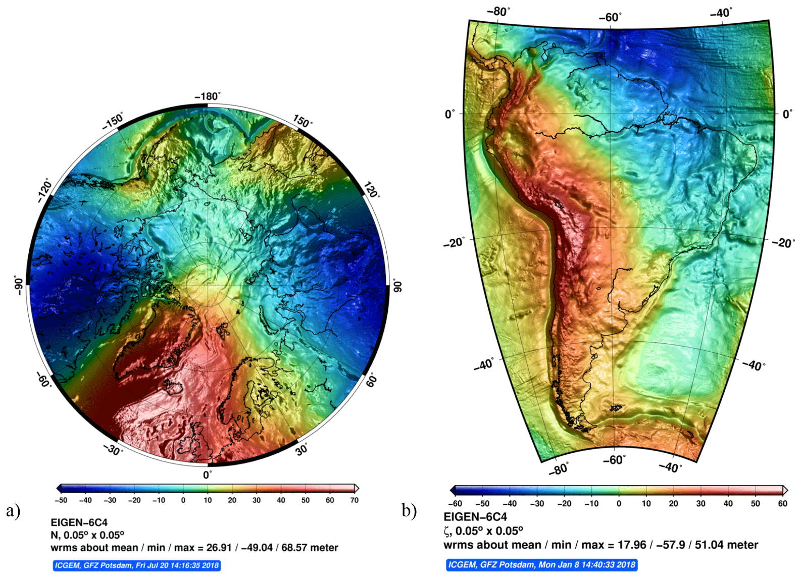
Figure A1Different projections are introduced in the background script which uses GMT version 5.0. The figures are adjusted based on the calculation area. The below figures show geoid undulations and height anomalies in (a) the Northern Hemisphere above 50 degrees latitude and (b) South America.
For the cross section calculation of the gravity field functionals along longitude, the figures below show (a) classical gravity anomalies at grid points where the red line indicated the cross section along longitude, (b) cross section classical gravity anomalies along longitude, and (c) cross section geoid undulations along longitude.
For the visualization of other celestial bodies, the figures below show geoid undulations of (a) the Moon, (b) Mars, and (c) Venus.
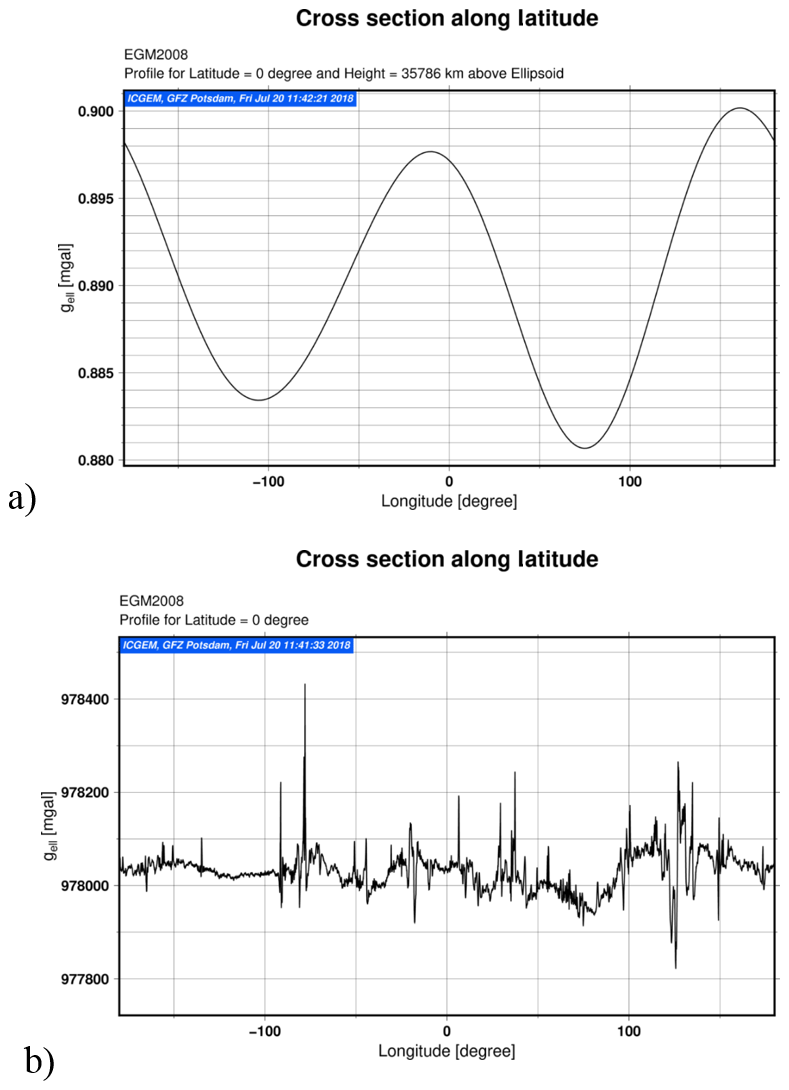
Figure A2Cross section calculation of gravity field functionals along latitude. The figures below show a cross section along the latitude of (a) gravity of a potential geostationary satellite at an altitude of approximately 36 000 km and (b) gravity on the Earth's surface along the equator.
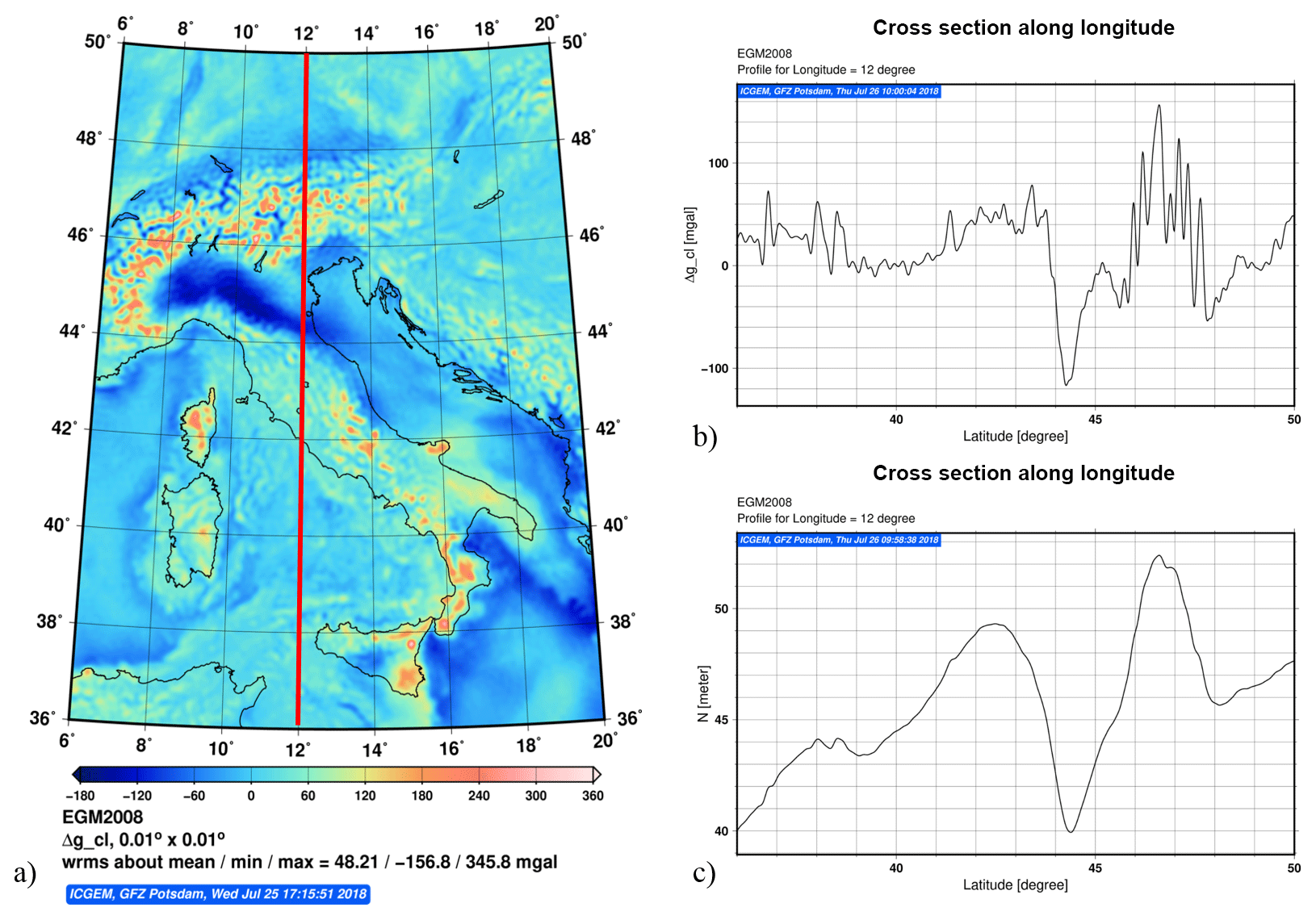
Figure A3Cross section calculation of the gravity field functionals along longitude. The figures below show (a) classical gravity anomalies at grid points where the red line indicated the cross section along longitude, (b) cross section classical gravity anomalies along longitude, and (c) cross section geoid undulations along longitude.

Figure A4Visualization of other celestial bodies. Panels show geoid undulations of (a) Moon, (b) Mars, and (c) Venus.
ESI is responsible for the maintenance and the development of the ICGEM service as of January 2018, prepared, and coordinated the manuscript. FB developed the software and tools used in the ICGEM service and contributed to the preparation and review of the manuscript. SR is responsible for the maintenance of the service together with ESI, does the web programming of the ICGEM service and contributed to the preparation of Sect. 5. KE developed the DOI services and is responsible for the DOI assignment for the models in the service, prepared Sect. 3.5 and reviewed the paper and suggested improvements. CF reviewed the paper in general and suggested improvements. FF reviewed the paper, especially Sect. 2.2.2, and suggested improvements. HS reviewed the IAG service and IUGG relevant parts and suggested improvements.
The authors declare that they have no conflict of interest.
We would like to acknowledge the past and present scientists who actively worked on the development of the ICGEM service as well as helped in its establishment. ICGEM would not be in its current stage without the contribution of Wolfgang Köhler. We would like to acknowledge his contributions in the development of 3-D visualization software since the beginning of the service until 2017. The founding fathers of the ICGEM service are Christoph Reigber and Peter Schwintzer (deceased 2005), who also established the funding for the ICGEM service. Christoph Dahle is acknowledged for his contributions in the temporal gravity-field-related components and Svetozar Petrovic for the delightful discussions during the evolution of ICGEM website. Christian Voigt, Damian Ulbricht, and Wouter van der Wal are thanked for reviewing a previous version of the paper. Lastly, as mentioned throughout the manuscript, user response, questions, and discussions with the ICGEM team significantly helped and are still helping to develop, improve, and further develop the tools. Therefore, we would like to especially acknowledge the user community that is contributing to the ICGEM's development with their questions, recommendations, and feedback. Finally, Generic Mapping Tools (GMTs) is acknowledged. The ICGEM service would not be in its current shape without the advanced and sophisticated GMT mapping tools. Last but not least, we would like to thank three anonymous referees who reviewed the paper and helped to improve the content and its readability.
This paper was edited by David Carlson and reviewed by three anonymous referees.
Barthelmes, F.: Definition of Functionals of the Geopotential and Their Calculation from Spherical Harmonic Models: Theory and formulas used by the calculation service of the International Centre for Global Earth Models (ICGEM), Scientific Technical Report STR09/02, Revised Edition, January 2013, Deutsches GeoForschungZentrum GFZ, https://doi.org/10.2312/GFZ.b103-0902-26, 2013.
Barthelmes, F.: Global Models, in: Encyclopedia of Geodesy, edited by: Grafarend, E., Springer International Publishing, 1–9, https://doi.org/10.1007/978-3-319-02370-0_43-1, 2014.
Barthelmes, F. and Förste, C: The ICGEM-format. Potsdam: GFZ German Research Centre for Geosciences, available at: http://icgem.gfz-potsdam.de/ICGEM-Format-2011.pdf (last access: 30 January 2019), 2011.
Barthelmes, F. and Koehler, W.: International Centre for Global Earth Models (ICGEM), in: Dreves: The Geodesists Handbook 2012, J. Geodesy, 86, 932–934, https://doi.org/10.1007/s00190-012-0584-1, 2012.
Barthelmes, F., Ince, E. S., and Reissland, S.: International Centre for Global Earth Models, International Association of Geodesy, Travaux, Volume 40, Reports 2015–2017, available at: https://iag.dgfi.tum.de/fileadmin/IAG-docs/Travaux_2015-2017.pdf (last access: 30 January 2019), 2017.
Bettadpur, B.: CSR Level-2 processing standards document for product release 05 GRACE 327–742, revision 4.0, 2012.
Cazenave, A., Dominh, K., Guinehut, S., Berthier, E., Llovel, W., Ramillien, G., Ablain, M., and Larnicol, G.: Sea level budget over 2003–2008: A reevaluation from GRACE space gravimetry, satellite altimetry and Argo, Global Planet. Change, 65, 83–88, https://doi.org/10.1016/j.gloplacha.2008.10.004, 2009.
Chao, C. C. G.: Applied orbit perturbation and maintenance, American Institute of Aeronautics and Astronautics, Inc., 2005.
Dahle, C., Flechtner, F., Gruber, C., König, D., König, R., Michalak, G., and Neumayer, K.-H.: GFZ GRACE Level-2 Processing Standards Document for Level-2 Product Release 0005, (Scientific Technical Report – Data; 12/02), Potsdam: Deutsches GeoForschungsZentrum GFZ, 20 p., https://doi.org/10.2312/GFZ.b103-12020, 2012.
Dahle, C., Murböck, M., Michalak, G., Neumayer, K. H., Flechtner, F., Abrykosov, O., Reinhold, A., and König, R.: The GFZ GRACE RL06 Time Series, EGU General Assembly, Vienna, Austria, 8–13 April 2018, EGU2018-17837, 2018.
Data Citation Synthesis Group: Joint Declaration of Data Citation Principles, edited by: Marttone, M., FORCE11, San Diego, https://doi.org/10.25490/a97f-egyk, 2014.
Drinkwater, M. R., Floberghagen, R., Haagmans, R., Muzi, D., and Popescu, A.: VII: CLOSING SESSION: GOCE: ESA's First Earth Explorer Core Mission, Space Sci. Rev., 108, 419–432, https://doi.org/10.1023/a:1026104216284, 2003.
Flechtner, F., Morton, P., Watkins, M., and Webb, F.: Status of the GRACE Follow-on Mission, in: Gravity, Geoid and Height Systems: Proceedings of the IAG Symposium GGHS2012, edited by: Marti, U., 9–12 October 2012, Venice, Italy, (International Association of Geodesy Symposia; 141), 2014.
Flechtner, F., Neumayer, KH., Dahle, C., Dobslaw, H., Fagiolini, E., Raimondo, J. C., and Güntner, A.: What can be expected from the GRACE-FO laser ranging interferometer for Earth science applications?, Surv. Geophys., 37, 263–280, https://doi.org/10.1007/s10712-015-9338-y, 2016.
Förste, C., Bruinsma, S., Abrikosov, O., Flechtner, F., Marty, J. C., Lemoine, J. M., and Biancale, R.: EIGEN-6C4-The latest combined global gravity field model including GOCE data up to degree and order 1949 of GFZ Potsdam and GRGS Toulouse, EGU General Assembly, Vienna, Austria, 27 April–2 May 2018, EGU2014-3707, 2014.
Förste, C., Bruinsma, S., Abrikosov, O., Rudenko, S., Lemoine, J. M., Marty, J. C., Neumayer, K. H., and Biancale, R.: EIGEN-6S4 A time-variable satellite-only gravity field model to d/o 300 based on LAGEOS, GRACE and GOCE data from the collaboration of GFZ Potsdam and GRGS Toulouse, GFZ Data Services, https://doi.org/10.5880/icgem.2016.004, 2016a.
Förste, C., Bruinsma, S., Abrikosov, O., Rudenko, S., Lemoine, J. M., Marty, J. C., Neumayer, K. H., and Biancale, R.: EIGEN-6S4 A time-variable satellite-only gravity field model to d/o 300 based on LAGEOS, GRACE and GOCE data from the collaboration of GFZ Potsdam and GRGS Toulouse. V. 2.0, GFZ Data Services, https://doi.org/10.5880/icgem.2016.008, 2016b.
Ghosh, A., Thyagarajulu, G., and Steinberger, B.: The Importance of Upper Mantle Heterogeneity in Generating the Indian Ocean Geoid Low, Geophys. Res. Lett., 44, 9707–9715, https://doi.org/10.1002/2017GL075392, 2017.
Gouweleeuw, B. T., Kvas, A., Gruber, C., Gain, A. K., Mayer-Gürr, T., Flechtner, F., and Güntner, A.: Daily GRACE gravity field solutions track major flood events in the Ganges-Brahmaputra Delta, Hydrol. Earth Syst. Sci., 22, 2867–2880, https://doi.org/10.5194/hess-22-2867-2018, 2018.
Grombein, T., K. Seitz, and Heck, B.: The Rock-Water-Ice topographic gravity field model RWI_TOPO_2015 and its comparison to a conventional rock-equivalent version, Surv. Geophys., 37, 937–976, https://doi.org/10.1007/s10712-016-9376-0, 2016.
Gruber, T.: Evaluation of the EGM2008 gravity field by means of GPS-levelling and sea surface topography solutions, External evaluation reports of EGM2008, Newton's Bulletin, Nr. 4, Bureau Gravimétrique International (BGI)/International Geoid Service (IGeS), ISSN 8555, 1810, 3–17, 2009.
Gruber, T., Visser, P. N. A. M., Ackermann, C., and Hosse, M.: Validation of GOCE gravity field models by means of orbit residuals and geoid comparisons, J. Geodesy, 85, 845–860, https://doi.org/10.1007/s00190-011-0486-7, 2011.
Hanson, B., Lehnert, K., and Cutcher-Gershenfeld, J.: Committing to Publishing Data in the Earth and Space Sciences, Eos, 96, https://doi.org/10.1029/2015eo022207, 2015.
Heiskanen, W. A. and Moritz, H.: Physical Geodesy, Bull. Géodés., (1946–1975), 86, 491–492, https://doi.org/10.1007/BF02525647, 1967.
Hirt, C. and Rexer, M.: Earth 2014: 1 arc-min shape, topography, bedrock and ice-sheet models – available as gridded data and degree 10 800 spherical harmonics, Int. J. Appl. Earth Observ. Geoinf., 39, 103–112, https://doi.org/10.1016/j.jag.2015.03.001, 2015.
Hirt, C., Rexer, M., Scheinert, M., Pail, R., Claessens, S., and Holmes, S.: A new degree-2190 (10 km resolution) gravity field model for Antarctica developed from GRACE, GOCE and Bedmap2 data, J. Geodesy, 90, 105–127, https://doi.org/10.1007/s00190-015-0857-6, 2016.
Hofmann-Wellenhof, B. and Moritz, H.: Physical geodesy, Springer Science & Business Media, 2006.
Huang, J. and Véronneau, M.: Assessments of recent GRACE and GOCE release 5 global geopotential models in Canada, Newton's Bull., 5, 127–148, 2015.
Ince, E. S., Sideris, M. G., Huang, J., and Véronneau, M.: Assessment of the GOCE-based global gravity models in Canada, Geomatica, June, 66, 125–140, https://doi.org/10.5623/cig2012-025, 2012.
Kotsakis, C., Katsambalos, K., and Gianniou, M.: Evaluation of EGM08 based on GPS and orthometric heights over the Hellenic mainland, Newton's Bulletin-External Quality Evaluation Reports of EGM08, April, 4, 144–163, 2009.
Kusche, J., Schmidt, R., Petrovic, S., and Rietbroek, R.: Decorrelated GRACE time-variable gravity solutions by GFZ, and their validation using a hydrological model, J. Geodesy, 83, 903–913, https://doi.org/10.1007/s00190-009-0308-3, 2009.
Lemoine, F. G., Kenyon, S. C., Factor, J. K., Trimmer, R. G., Pavlis, N. K., Chinn, D. S., Cox, C. M., Klosko, S. M., Luthcke, S. B., Torrence, M. H., and Wang, Y. M.: The development of the joint NASA GSFC and the National Imagery and Mapping Agency (NIMA) geopotential model EGM96, NASA/TP-1998-206861, available at: https://ntrs.nasa.gov/archive/nasa/casi.ntrs.nasa.gov/19980218814.pdf (last access: 6 May 2019), 1998.
Li, X., Crowley, J. W., Holmes, S. A., and Wang, Y. M.: The contribution of the GRAV-D airborne gravity to geoid determination in the Great Lakes region, Geophys. Res. Lett., 43, 4358–4365, https://doi.org/10.1002/2016GL068374, 2016.
Mayer-Gürr, T.: ITG-Grace03s: the latest GRACE gravity field solution computed in Bonn, in: Presentation at the joint international GSTM and SPP symposium, Potsdam, Germany, 15–17 October, 2007.
Mayer-Gürr, T., Pail, R., Gruber, T., Fecher, T., Rexer, M., Schuh, W.-D., Kusche, J., Brockmann, J.-M., Rieser, D., Zehentner, N., Kvas, A., Klinger, B., Baur, O., Hoeck, E., Krauss, S., and Jaggi, A.: The combined satellite gravity field model GOCO05s; EGU General Assembly, Vienna, Austria, 12–17 April, EGU2015-12364, 2015.
Mayer-Gürr, T., Behzadpur, S., Ellmer, M., Kvas, A., Klinger, B., Strasser, S., and Zehentner, N.: ITSG-Grace2018 – Monthly, Daily and Static Gravity Field Solutions from GRACE, GFZ Data Services, https://doi.org/10.5880/ICGEM.2018.003, 2018.
Moritz, H.: Advanced physical geodesy, Advances in Planetary Geology, Wichmann, Karlsruhe, Germany, 1980.
Mularie, W.: Department of defense world geodetic system 1984, its definition and relationships with local geodetic systems, National Geospatial-Intelligence Agency, Tech. Rep, 152, 2000.
Oldenburg, D. W., Li, Y., Farquharson, C. G., Kowalczyk, P., Aravanis, T., King, A., Zhang, P., and Watts, A.: Applications of geophysical inversions in mineral exploration, The Leading Edge, 17, 461–465, https://doi.org/10.1190/1.1437989, 1998.
Pail, R., Fecher, T., Barnes, D., Factor, J. F., Holmes, S. A., Gruber, T., and Zingerle, P.: Short note: the experimental geopotential model XGM2016, J. Geodesy, 92, 443–451, https://doi.org/10.1007/s00190-017-1070-6, 2018.
Pavlis, N. K., Holmes, S. A., Kenyon, S. C., and Factor, J. K.: The development and evaluation of the Earth Gravitational Model 2008 (EGM2008), J. Geophys. Res.-Solid Earth, 117, B04406, https://doi.org/10.1029/2011JB008916, 2012.
Reigber, C., Lühr, H., and Schwintzer, P.: CHAMP mission status, Adv. Space Res., 30, 129–134, https://doi.org/10.1016/S0273-1177(02)00276-4, 2002.
Rexer, M., Hirt, C., Claessens, S., and Tenzer, R.: Layer-based modelling of the Earth's gravitational potential up to 10-km scale in spherical harmonics in spherical and ellipsoidal approximation, Surv. Geophys., 37, 1035–1074, https://doi.org/10.1007/s10712-016-9382-2, 2016.
Rummel, R. and Sansò, F.: Satellite Altimetry in Geodesy and Oceanography, Lecture Notes in Earth Sciences 50, Springer-Verlag Berlin Heidelberg, https://doi.org/10.1007/BFb0117924, 1993.
Rummel, R., Yi, W., and Stummer, C.: GOCE gravitational gradiometry, J. Geodesy, 85, 777, https://doi.org/10.1007/s00190-011-0500-0, 2011.
Save, H., Tapley, B., and Bettadpur, S.: GRACE RL06 reprocessing and results from CSR. EGU General Assembly, Vienna, Austria, 8–13 April 2018, EGU2018-10697-1, 2018.
Schmidt, R., Schwintzer, P., Flechtner, F., Reigber, C., Güntner, A., Döll, P., and Wünsch, J.: GRACE observations of changes in continental water storage, Global Planet. Change, 50, 112–126, https://doi.org/10.1016/j.gloplacha.2004.11.018, 2006.
Sideris, M. and Fotopoulos, G.: Special Issue on Regional and Global Geoid-based Vertical Datums, J. Geodetic Sci., 2, https://doi.org/10.2478/jogs-2013-0006, 2012.
Siemes, C.: Improving GOCE cross-track gravity gradients, J. Geodesy, 92, 33–45, https://doi.org/10.1007/s00190-017-1042-x, 2018.
Tapley, B. D., Bettadpur, S., Ries, J. C., Thompson, P. F., and Watkins, M. M.: GRACE measurements of mass variability in the Earth system, Science, 305, 503–505, https://doi.org/10.1126/science.1099192, 2004.
Velicogna, I.: Increasing rates of ice mass loss from the Greenland and Antarctic ice sheets revealed by GRACE, Geophys. Res. Lett., 36, L19503, https://doi.org/10.1029/2009GL040222, 2009.
Wahr, J. M.: Time variable gravity from satellites, Treatise Geophys., 3 213–237, https://doi.org/10.1016/B978-044452748-6.00176-0, 2007.
Wahr, J., Molenaar, M., and Bryan, F.: Time variability of the Earth's gravity field: Hydrological and oceanic effects and their possible detection using GRACE, J. Geophys. Res.-Solid Earth, 103, 30205–30229, https://doi.org/10.1029/98JB02844, 1998.
Wahr, J., Swenson, S., Zlotnicki, V., and Velicogna, I.: Time variable gravity from GRACE: First results, Geophys. Res. Lett., 31, L11501, https://doi.org/10.1029/2004GL019779, 2004.
Watkins, M. M. and Yuan, D. N.: JPL Level-2 processing standards document for Level-2 product release 05, GRACE Document, 327–744, available at: ftp://isdcftp.gfz-potsdam.de/grace/DOCUMENTS/Level-2/GRACE_JPL_L2_Processing_Standards_Document_for_RL05.pdf (last access: 31 January 2019), 2012.
Weigelt, M., van Dam, T., Jäggi, A., Prange, L., Tourian, M. J., Keller, W., and Sneeuw, N.: Time-variable gravity signal in Greenland revealed by high-low satellite-to-satellite tracking, J. Geophys. Res.-Solid Earth, 118, 3848–3859, https://doi.org/10.1002/jgrb.50283, 2013.
Wessel, P. and Smith, W. H.: New, improved version of Generic Mapping Tools released. Eos, Trans. Am. Geophys. Union, 79, 579–579, https://doi.org/10.1029/98EO00426, 1998.
Wessel, P., Smith, W. H., Scharroo, R., Luis, J., and Wobbe, F.: Generic mapping tools: improved version released, Eos, Trans. Am. Geophys. Union, 94, 409–410, https://doi.org/10.1002/2013EO450001, 2013.
Wieczorek, M. A.: Gravity and topography of the terrestrial planets, Treat. Geophys., 10, 165–206, https://doi.org/10.1016/B978-044452748-6.00156-5, 2015.
Yuan, D.: JPL level-2 processing standards document for level-2 product release 06, Jet Propulsion Laboratory, California Institute of Technology, 2018.
Zuber, M. T., Smith, D. E., Watkins, M. M., Asmar, S. W., Konopliv, A. S., Lemoine, F. G., Melosh, H. J., Neumann, G. A., Phillips, R. J., Solomon, S. C., and Wieczorek, M. A.: Gravity field of the Moon from the Gravity Recovery and Interior Laboratory (GRAIL) mission, Science, 339, 668–671, https://doi.org/10.1016/B978-044452748-6.00156-5, 2013.