the Creative Commons Attribution 4.0 License.
the Creative Commons Attribution 4.0 License.
 | 09 Jan 2019
Two multi-temporal datasets that track the enhanced landsliding after the 2008 Wenchuan earthquake
Gianvito Scaringi
Guillem Domènech
Lanxin Dai
Chaoyang He
Qiang Xu
Runqiu Huang
We release two datasets that track the enhanced landsliding induced by the 2008 Mw 7.9 Wenchuan earthquake over a portion of the Longmen Mountains, at the eastern margin of the Tibetan Plateau (Sichuan, China). The first dataset is a geo-referenced multi-temporal polygon-based inventory of pre- and coseismic landslides, post-seismic remobilisations of coseismic landslide debris and post-seismic landslides (new failures). It covers 471 km2 in the earthquake's epicentral area, from 2005 to 2018. The second dataset records the debris flows that occurred from 2008 to 2017 in a larger area (∼17 000 km2), together with information on their triggering rainfall as recorded by a network of rain gauges. For some well-monitored events, we provide more detailed data on rainfall, discharge, flow depth and density. The datasets can be used to analyse, on various scales, the patterns of landsliding caused by the earthquake. They can be compared to inventories of landslides triggered by past or new earthquakes or by other triggers to reveal common or distinctive controlling factors. To our knowledge, no other inventories that track the temporal evolution of earthquake-induced mass wasting have been made freely available thus far. Our datasets can be accessed from https://doi.org/10.5281/zenodo.1405489. We also encourage other researchers to share their datasets to facilitate research on post-seismic geological hazards.
- Article
(28243 KB) - Full-text XML
- BibTeX
- EndNote


1.1 Earthquake-induced enhanced landsliding
Large earthquakes cause major disturbances to the patterns of erosion and sediment export from mountain belts (e.g. Keefer, 1994; Dadson et al., 2004; Hovius et al., 2011; Parker et al., 2011; Huang and Fan, 2013; Li et al., 2017). Thousands of landslides can be triggered by seismic shaking. These coseismic landslides generate large amounts of debris, part of which will reach large streams and form landslide-dammed lakes that impound large volumes of water and sediments (Fan et al., 2012, 2017b; Tang et al., 2018). More debris will deposit, with marginal stability, high on the slopes and in low-order channels (Meunier et al., 2008; Gorum et al., 2011; Kargel et al., 2016; Fan et al., 2018a, b). It will be remobilised easily by minor storms (Dadson et al., 2004; Lin et al., 2006; Huang and Fan, 2013; Fan et al., 2018b) and generate large flow-like landslides (Xu et al., 2012; Hu et al., 2017). The earthquake-induced enhanced weakening and weathering of rock and soil masses will also cause delayed slope failures and sustain high erosion rates for a long time (Koi et al., 2008; Parker et al., 2015; Fan et al., 2017a, 2018d; Scaringi et al., 2018). These processes are a major source of hazard to the population and infrastructure. Earthquake-triggered chains of geohazards are major contributors to the tolls of damage and fatalities and to the costs of reconstruction and recovery of the socioeconomic fabric after large earthquakes (Huang and Fan, 2013; Wang et al., 2014).
Observations on the evolution of mass wasting after recent major earthquakes reveal a peak of landslide rates (remobilisations of coseismic landslide deposits and post-seismic landslides) soon after the earthquakes, followed by decay and normalisation within less than a decade (Fan et al., 2018a; Hovius et al., 2011; Marc et al., 2015; Zhang et al., 2016; Zhang and Zhang, 2017). The reasons for this normalisation, which seems quicker than that of the sediment export by non-landslide processes (Ding et al., 2014; Wang et al., 2015, 2017), are still poorly understood. Various processes, such as the progressive depletion of the debris, grain coarsening and densification, restoration of the vegetation cover and bedrock healing have been shown to play a role (e.g. Shieh et al., 2009; Zhang et al., 2014; Yang et al., 2018). Analyses of complete inventories that track the decay of landslide rates, together with laboratory and field-scale investigations and physically based models, can certainly provide further insights.
1.2 Multi-temporal inventorying of landslides
Landslide mapping and inventorying on various scales are fundamental tools with which to investigate the spatial and temporal patterns of mass movements quantitatively, obtain insight into their failure-run-out mechanisms and damage, and reveal topographic, seismic, geological, hydrological, climatic, biological and anthropogenic preconditions and causal factors on their distribution and fate (e.g. Guzzetti et al., 2002, 2009, 2012; Corominas et al., 2014; Galli et al., 2008; Harp et al., 2011; Parker et al., 2015; Gariano and Guzzetti, 2016; Broeckx et al., 2018). Coseismic landslide inventories are compiled after major events with increasing quality and completeness (Keefer, 2002; Schmitt et al., 2017; Tanyaş et al., 2017). They are fundamental for assessing the extent of the earthquake-affected areas and drive the post-earthquake emergency response, as they are the basis for susceptibility, hazard and risk analyses. Additionally, they can help reconstruct earthquake mechanisms (Gorum et al., 2011; Fan et al., 2018c). For instance, studies by Keefer (1984) and Rodriguez et al. (1999) first related the spread of landslides from the seismogenic fault to the earthquake magnitude. Besides, complete and detailed inventories are necessary to evaluate the landscape response to earthquakes quantitatively and to calibrate descriptive and predictive models effectively (Xu et al., 2014; Marc and Hovius, 2015; Marc et al., 2016a, b, 2017). Many coseismic landslide inventories have been released, and some of them were collected in a freely accessible repository by Schmitt et al. (2017). We believe that this important step will promote the standardisation of data collection and presentation, and facilitate meta-analyses and modelling efforts greatly. Several inventories were compiled for the Wenchuan earthquake-affected area (Gorum et al., 2011; Dai et al., 2011; Xu et al., 2014; Li et al., 2014; Tang et al., 2016). Landslides were mapped either as points (identifying the landslide scar) or polygons, with different degrees of accuracy (see Tang et al., 2016) and with or without distinction between landslide types (slides, flows, etc.). Both accuracy and representation (as points or polygons) have direct implications for the analysis of landslide size-frequency distributions and hazard and risk assessments, as well as for the analysis of controlling factors. Additionally, the distinction between different types of landslide allows for dedicated analyses of distinctive controlling factors and characteristics.
Landslide inventories that include several temporal scenes before and after earthquakes are much less common. In fact, the interest around the temporal evolution of landsliding after major earthquakes has increased greatly in the past decades, particularly after the 1999 Mw 7.7 Chi-Chi and 2008 Mw 7.9 Wenchuan earthquakes (Dadson et al., 2004; Fan et al., 2018a, b; Hovius et al., 2011; Marc et al., 2015; Tang et al., 2016; Yang et al., 2017, 2018; Zhang et al., 2016; Zhang and Zhang, 2017) and has the potential to answer various research questions concerning, for instance, erosional patterns and morphological signatures in seismically active mountain ranges. Research has been facilitated by the increased availability of repeated and high-resolution remote-sensing images (Fan et al., 2018b) and by near-real-time monitoring networks (Huang et al., 2015). However, to our knowledge, none of the multi-temporal inventories of post-seismic landslides compiled so far have been released to open repositories. With this paper and the related datasets, we wish to share our mapping work and monitoring data to facilitate further analyses and meta-analyses by the research community. We also wish to encourage other researchers to publish their data, with the aim of building a collection of datasets that will help advance knowledge in the field.
Our datasets cover portions of the region affected by the Mw 7.9 Wenchuan earthquake at various levels of detail (Fig. 1). The earthquake hit the Longmen Mountains (Longmenshan) in western Sichuan, China, at the eastern margin of the Tibetan Plateau on 12 May 2008, with a fault rupture that propagated from the epicentre along the range for about 240 km (Gorum et al., 2011; Huang and Fan, 2013; Fan et al., 2018b). Details on the tectonic setting of the Longmenshan and on the Wenchuan earthquake mechanisms, as well as geological and geomorphological characterisations of the region, can be found in several earlier works (Qi et al., 2010; Dai et al., 2011; Gorum et al., 2011) to which the reader is referred for further information.
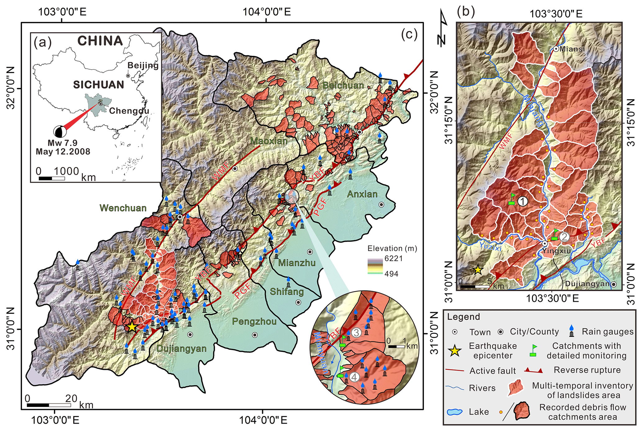
Figure 1General view of the study area in Sichuan, China (a). Detail of the area in which the multi-temporal inventory of landslides was carried out (b). Detail of the area in which debris flows were recorded, with an indication of their location and those of the rain gauges (c). Circled numbers (1–4) indicate well-monitored catchments.
According to a recent inventory (Xu et al., 2014), the Wenchuan earthquake triggered almost 200 000 coseismic landslides over a region larger than 110 000 km2. The total landslide area was estimated in about 1160 km2 (Xu et al., 2014), and the total landslide volume was in the order of several km3 (Parker et al., 2011; Li et al., 2014; Marc and Hovius, 2015; Xu et al., 2014, 2016). Rain-induced post-seismic failures of deposits of coseismic debris, often evolving into catastrophic debris flows and floods, have been occurring frequently after the earthquake (Tang et al., 2009, 2011, 2012; Xu et al., 2012; Guo et al., 2016, 2017).
2.1 Inventory of landslides
Our multi-temporal inventory of pre- and coseismic landslides, post-seismic remobilisations and new failures covers a significant portion of the earthquake's epicentral area. It is the largest area affected by the Wenchuan earthquake that has been covered by a detailed multi-temporal landslide inventory thus far (Fan et al., 2018a). The area comprises 42 catchments over 471 km2 from the town of Yingxiu (the epicentre) to the town of Wenchuan (Fig. 1b). It has been affected by coseismic landslides with a total volume in the range 0.8–1.5 billion m3, as estimated through a set of first-order empirical area–volume scaling relationships (Parker et al., 2011; Xu et al., 2016). The reader is referred to Fan et al. (2018c) for a discussion on the reliability and uncertainties arising from the use of empirical area–volume relationships for the estimation of coseismic landslide volumes.
The region that we investigated has rugged mountains with elevations that rise rapidly from 420 m a.s.l. in the main river valley to over 4000 m a.s.l. of some mountain ridges. The slopes are generally steep, with more than half of them steeper than 36∘. Two of the main faults of the Longmenshan, the Wenchuan–Maowen and the Yingxiu–Beichuan faults (e.g. Qi et al., 2010), delimit this study area. Beneath dense vegetation and a variably thick soil cover lie weathered and highly fractured rocks, mostly igneous (granite, diorite), though metamorphic and sedimentary rocks (schist, shale, sandstone, limestone) are also present, as well as recent Quaternary deposits. The climate is subtropical, affected by the monsoonal circulation, with 13 ∘C of mean annual temperature and >1250 mm year−1 of precipitation which mostly occurs in the summer months. The Min River (Minjiang), a tributary of the Yangtze River in its upper course, crosses the region through Wenchuan and Yingxiu and discharges, on average throughout the year, 452 m3 s−1 of water (Tang et al., 2011).
2.2 Inventory of debris flows and their triggering rainfalls
The dataset of debris flows and their triggering rainfalls covers 16 959 km2, from the epicentre (near the town of Yingxiu) to the edge of the thrust-dominated portion of the seismogenic fault rupture (near the town of Beichuan). In this region, 527 debris flows affecting 244 catchments were identified. These catchments cover about 1581 km2 altogether (Fig. 1c) and spread along 177 km out of the 246 km of the fault surface rupture.
The study area is mountainous with elevations from 420 m a.s.l. in the river valley up to almost 6100 m a.s.l. on the ridges of the Hengduan Mountains. A general northeast-to-southwest orientation is shown by the geological structures and the strike of the rock strata, and the bedrock outcrops are highly fractured and weathered. Most of the low-order channels are deeply cut and the slopes are steep, with a morphology that is strongly controlled by the high tectonic activity (Guo et al., 2016). The climate is generally monsoon influenced, with precipitation concentrated in the summer months. However large variability exists within this larger region, with the central and southern parts receiving annual precipitations exceeding 1200 mm and easily reaching 2000 mm, and the western part being drier and receiving less than 800 mm year−1 of precipitation (Guo et al., 2016).
The complex geology and the patterns of precipitation (with frequent but localised rainstorms that can deliver hundreds of millimetres of rain in each event) make the area highly prone to the occurrence of debris flows. About 250 debris flows were recorded in the decades preceding the Wenchuan earthquake (Cui et al., 2008), and hundreds more were triggered after the earthquake, affecting more than 800 streams within the first 2 years (Cui et al., 2011). The characteristics of the rain events that triggered debris flows changed abruptly with the earthquake, with triggering rainfall intensity and duration that dropped significantly and subsequently exhibited a pattern of gradual recovery over a decadal timescale (e.g. Yu et al., 2014; Guo et al., 2016, 2017).
Here we provide details of the source data and the preparation of our inventories. We also include some figures and tables that illustrate the contents of the inventories and some simple analyses.
3.1 Multi-temporal inventory of landslides
3.1.1 Imagery, mapping technique, attributes
We compiled the inventory through visual interpretation (following Harp et al., 2011) of high-resolution aerial and satellite images (Spot 5, Spot 6, Worldview 2, Pleiades). In total, eight sets of images were acquired, covering the period from 2005 to 2018 (Table 1). We selected these scenes according to the availability, date of acquisition, coverage, absence of clouds and resolution. With respect to the targeted study region, the areal coverage of the images is close to 99 % in 2007, 2011 and 2015, 97 % in 2008, 95 % in 2013, and 93 % in 2005, 2017 and 2018. The 2011 scene was used as our geo-referencing base in the ArcGIS environment (Environmental Systems Research Institute, Inc., United States) and the orthorectification was performed using the software Pix4D (Pix4D S.A., Switzerland). A 25 m resolution digital elevation model, obtained from the Sichuan Bureau of Surveying and Mapping, was used to delineate the catchment boundaries.
Table 1Reference images used to map the landslides, acquisition date and attributes of each layer contained in the dataset. An additional shape file is provided to define the catchment boundaries and have a simple characterisation (CID: catchment identifier, catchment name and county, gradient and internal relief, drainage density and channel length).
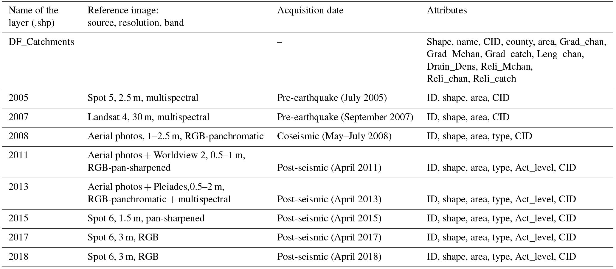
Attributes: shape (type of element: polygon, line, point), name (name of each catchment), CID (identifier for each catchment), county (name of the administrative county where the catchment is located), area (area of each element in m2), Grad_chan (mean slope of the whole channels present in the catchment in decimal degrees), Grad_Mchan (mean slope of the main channel present in the catchment in decimal degrees), Grad_catch (mean slope of the catchment in decimal degrees), Leng_chan (total length of the channels present in the catchment in metres), Drain_Dens (Leng_chan/Area in m−1), Reli_Mchan (relief of the main channel: highest altitude minus lowest altitude of the main channel in metres), Reli_chan (relief of all the channels present in the catchment: highest altitude minus lowest altitude of the channels in metres), Reli_catch (relief of the catchment: highest altitude minus lowest altitude of the catchment in metres), ID (identifier of each element), type (type of landslide: s – slide, d – debris flow, cd – channel deposit), Act_level (level of activity of the landslide: 0 – activity level A0, dormant landslide, 1 – activity level A1, 2 – activity level A2, 3 – activity level A3, 4 – new landslide).
Our inventory (Figs. 2, 3) provides a polygon-based delineation of landslides that occurred before the earthquake (2005 and 2007 scenes), which can be used to define the pre-earthquake landslide rates and patterns in studies focusing on a short-term time window. The 2008 scene was used to delineate the coseismic landslides; the 2011, 2013, 2015, 2017 and 2018 scenes were used to identify the new landslides that occurred after the earthquake (i.e. the post-seismic landslides) and the remobilisations of coseismic landslides (i.e. the post-seismic remobilisations).
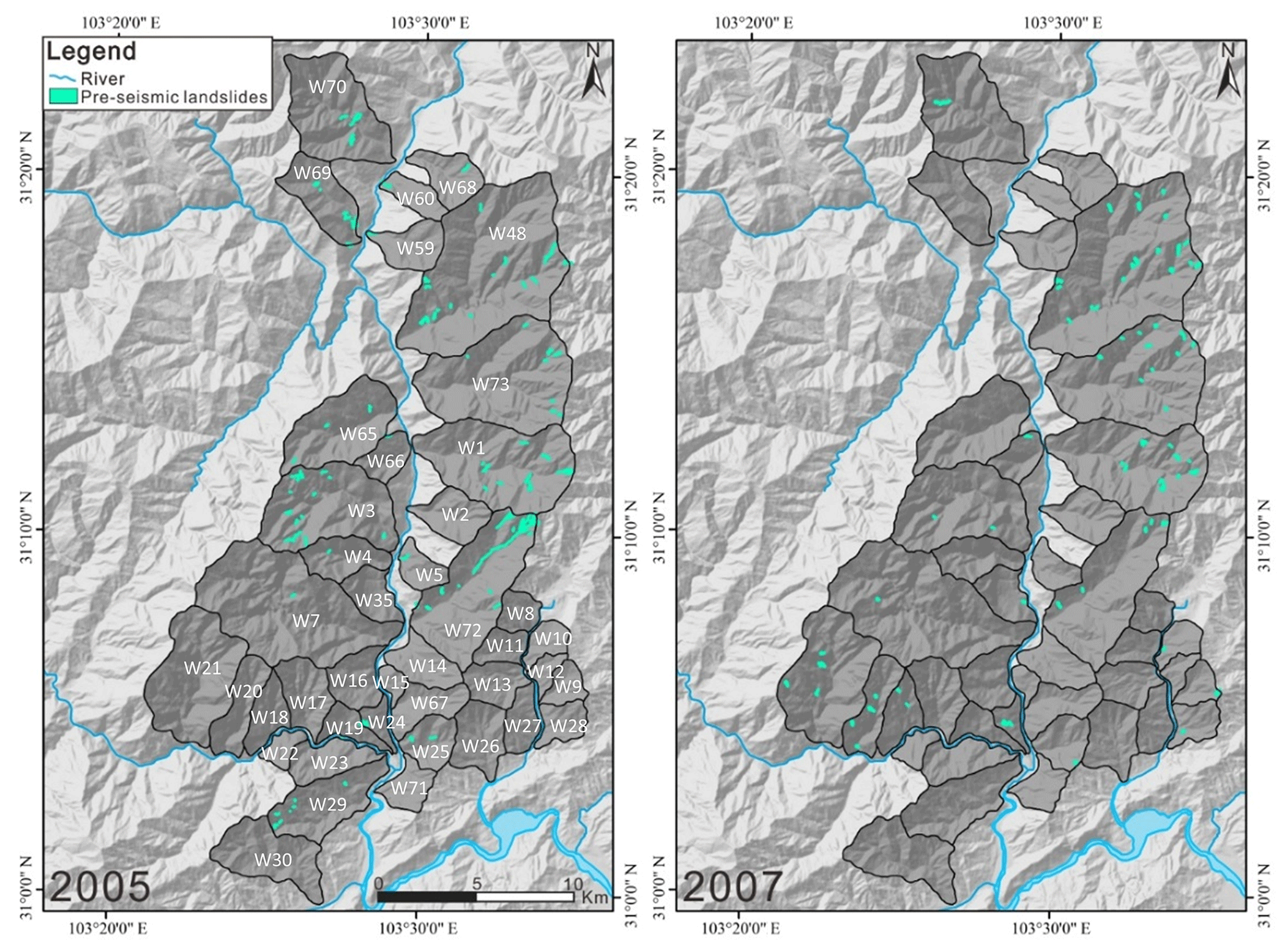
Figure 2Landslides identified from remote-sensing images recorded in 2005 and 2007 (pre-earthquake). The identifier for each catchment (see CID in Table 1) is shown in 2005.
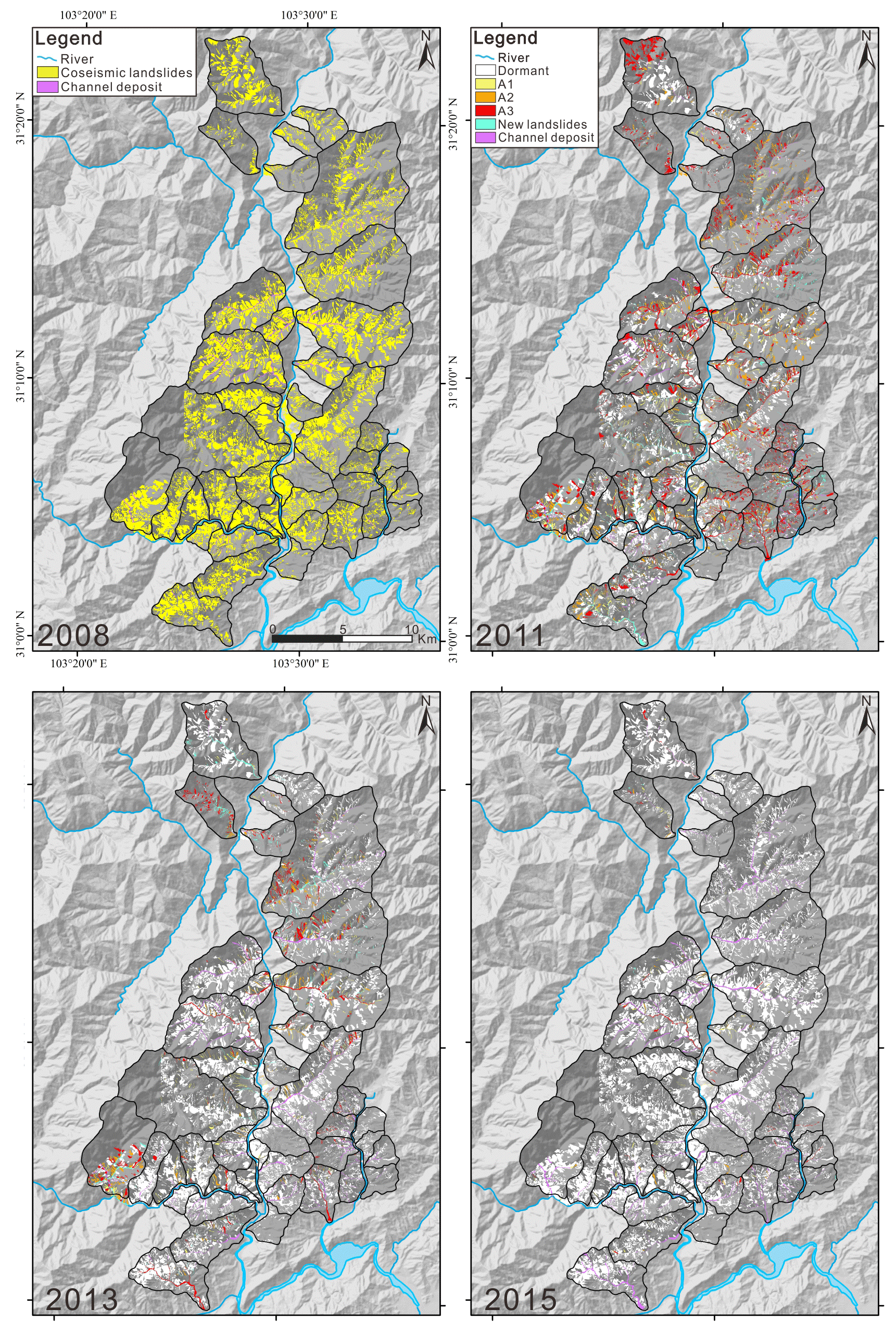
Figure 3Coseismic landslides, post-seismic remobilisation of coseismic landslide deposits and post-seismic landslides (new landslides) identified from remote-sensing images recorded in 2008, 2011, 2013, 2015, 2017 and 2018. For the remobilisations, the levels of activity are also indicated.
The landslide areas were differentiated into three types: slides, debris flows and channel deposits. Slides were mapped as if preferential movement paths could not be identified in their debris-covered deposition areas. This type comprises debris and rockslides and debris and rockfalls (see Hungr et al., 2014, for the definitions of the landslide types). This simplification derives from a lack of discernibility, in the remote-sensing images, between these types of movement and their combinations. In contrast, debris flows exhibited a finer material texture along a preferential movement path. They were found along the hillslopes (hillslope debris flows) and into small channels (channelised debris flows). Large amounts of accumulated debris were also found in the main channels. The source area of these materials is not known as they come from multiple debris flows and slides located upstream, and in many cases clear remobilisations could not be identified. Therefore, these deposits were mapped as channel deposits. They are very important source areas for subsequent debris flows initiated by run-off erosion during intense storms. Some examples of landslide types are given in Fig. 4.
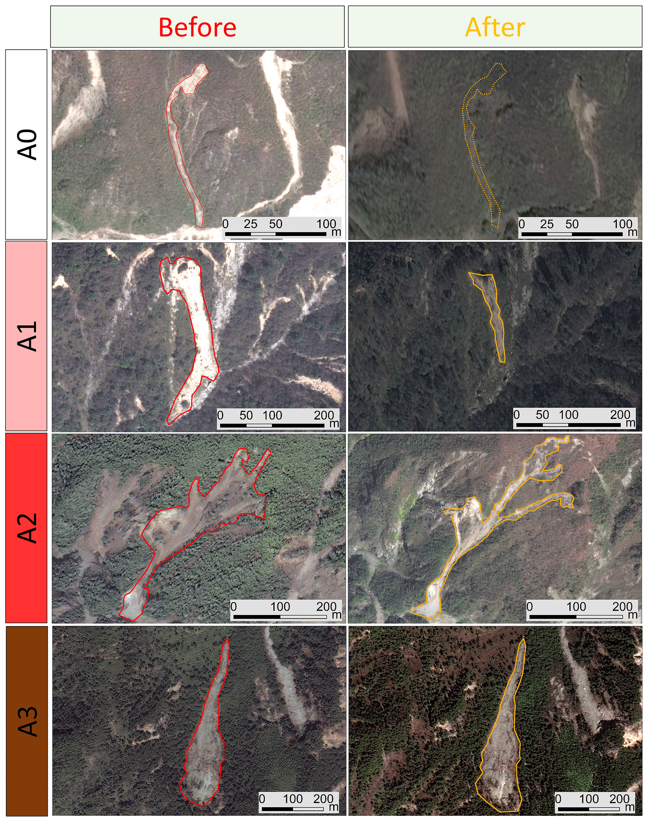
It is worth noting that, in contrast to earlier works (Tang et al., 2016; Yang et al., 2017; Zhang et al., 2016), we quantified changes of the level of activity based on the actual polygon-mapping of the remobilised areas (Fig. 5), discriminated between different types of landslides and their location and investigated a much larger and more representative area. Nevertheless, for ease of visualisation and comparison of some results (see Figs. 3 and 6), we defined four levels of activity to classify the landslide remobilisations, following Tang et al. (2016). A level of activity A1 was assigned if less than one-third of the coseismic or post-seismic landslide area displayed signs of remobilisation; a level A2 was assigned if the remobilisation involved between one-third and two-thirds of the area; a level A3 was assigned if the remobilisation involved more than two-thirds of the area. Finally, a level A0 was assigned if no remobilisations were identified (i.e. the landslide was dormant or its movement was too slow to produce changes that could be seen from the available imagery).
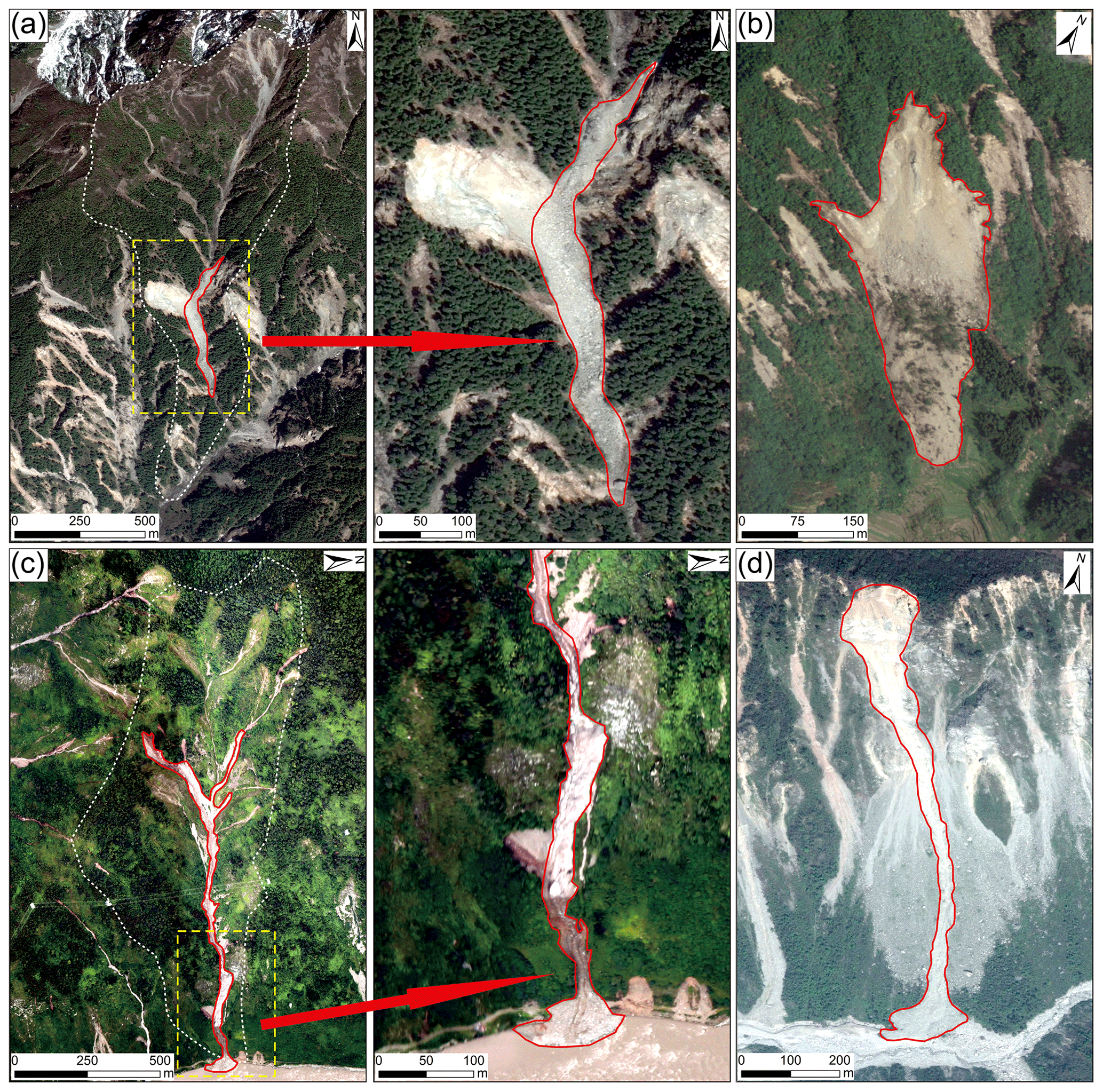
Figure 4Types of landslides and deposits mapped in the inventory: channel deposit (a), slide (b), debris flow in a channel (c) and debris flow on a hillslope (d).
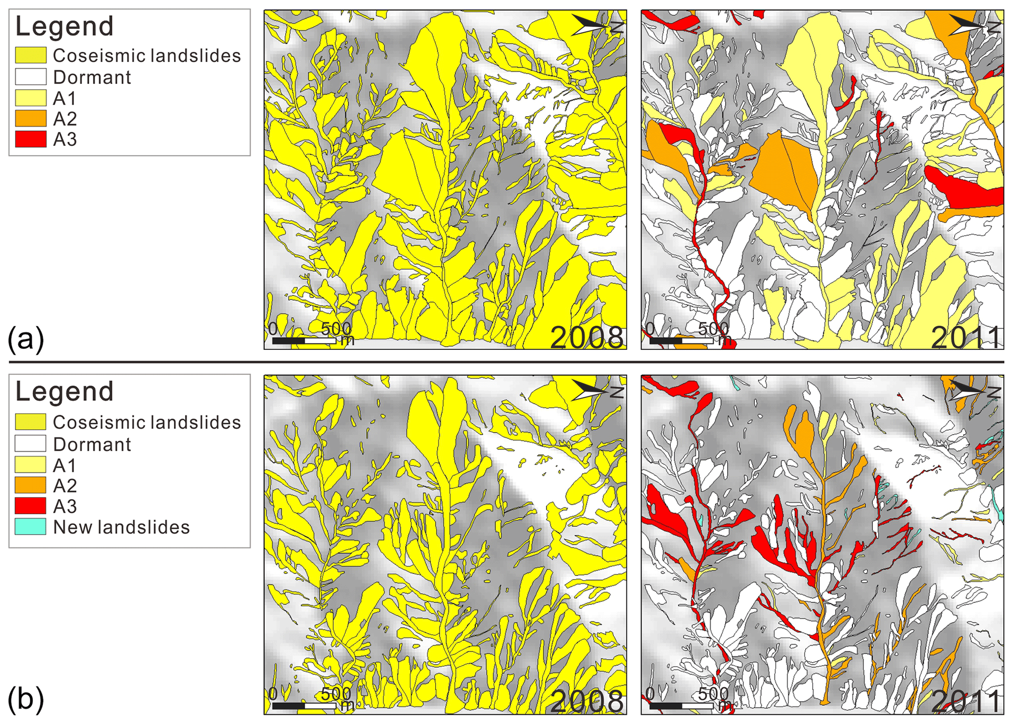
Figure 5Comparison between the landslide mapping by Tang et al. (2016) and that of the present work in a portion of the study area, using the remote-sensing scene recorded in 2011. Note that Tang et al. (2016) use the polygons delineating the coseismic landslides (2008 scene) and estimate the proportion of landslide area remobilised as of 2011, providing this estimation in the attributes table of the map. Conversely, in this work the remobilised areas were remapped with new polygons in each post-earthquake scene. In this way, not only can the remobilised area be calculated, but the spatial characteristics of the remobilisations can also be studied.
3.1.2 Uncertainties
The processes of manual mapping and discernment of landslide boundaries and types are obviously affected by unavoidable uncertainties due to stochastic errors and systematic biases, such as the variable quality of the remote-sensing images, and the variable experience of the mappers. Nevertheless, we preferred this approach because, on the other hand, semi-automatic and automatic methods of landslide identification do not necessarily offer better performances and can even lead to larger uncertainties when applied to very high-resolution images (van Westen et al., 2006; Guzzetti et al., 2012; Pawłuszek et al., 2017). Moreover, some semi-automatic techniques still need visual interpretation over a significant test area for calibration (e.g. Đurić et al., 2017), and automatic methods may require a combination of images of different portions of the spectrum or of satellite and aerial images that should be acquired within a narrow time window to be significant for a multi-temporal inventorying of fast-evolving features. Such techniques are not necessarily less time consuming than the manual interpretation (Santangelo et al., 2015).
Our mapping was carried out by five mappers, who worked on distinct areas with the same set of pre-agreed rules for the identification of the landslides and their types (see also Fan et al., 2018a). The mappers worked in close contact, interacting and discussing non-easily-discernible cases. Nonetheless, we evaluated the individual performances of the mappers to make an estimation of the mapping uncertainties and their propagation into further analyses. We selected a test area (a portion of a catchment), on which accurate mapping had been performed for one scene (2011), which was verified and improved during field investigation. We assumed the landslide inventory for this test area to be good enough to consider the uncertainties negligible, and we used it as a reference. We asked each mapper to produce, independently, an inventory of the same area, which we compared to the reference inventory (Fig. 7). We evaluated the matching degree between each mapper's inventory and the reference inventory, Mn, which we defined as follows:
where An is the landslide area delineated by the nth mapper, Ar is the respective area of the reference inventory, and An⋂Ar is the intersection of the two areas, i.e. the portion in which they match. We then calculated the average matching degree of the team as follows:
where N is the number of mappers in the team. A matching degree was evaluated in the test area. On average, the landslide areas matched those of the reference inventory by 76 %, and an average mapping uncertainty of ±19 % in terms of the total landslide area was calculated. If this same value of uncertainty is assumed for the entire study area, this will be a conservative estimate, as the uncertainties will tend to decrease with the landslide areas increasing, and the test area consisted mostly of small landslides. We believe that this uncertainty can be acceptable when performing regional-scale analyses, as it can be demonstrated that it does not affect the patterns of frequency-size distributions or potential controlling factors significantly (Fan et al., 2018a).

Figure 7Landslide inventory of a test area (remote-sensing image recorded in 2011): comparison between the reference, field-checked inventory with those produced by five mappers (a–e) independently, on the basis of the sole imagery and a common set of rules. Darker shades indicate areas in which most inventories overlap.
3.1.3 Descriptive statistics
We identified 133 and 71 landslides in the 2005 and 2007 (pre-earthquake) scenes, and 8917 coseismic landslides in the 2008 scene, of which 8259 were classified as slides, 571 as debris flows and 87 as channel deposits. We also delineated 832 new landslides in the 2011 scenes (589 slides, 193 debris flows, 50 channel deposits), 387 in the 2013 scene (254 slides, 106 debris flows, 27 channel deposits), 14 in the 2015 scene (7 slides, 1 debris flow, 6 channel deposits), 5 in the 2017 scenes (2 slides, 2 debris flows, 1 channel deposit), and 9 (all slides) in the 2018 scene. In the 2011, 2013, 2015, 2017 and 2018 scenes we identified 4099, 1152, 273, 22 and 29 remobilised landslides (having levels of activity A1–A3). More details are given in Table 2. Note that some of these numbers differ from those published by Fan et al. (2018a) for the period until 2015, even though they referred to the same study area, because the inventory has been refined and improved since then.
Table 2Landslides with no information (NI), channel deposits (cd), slides (s), debris flows (d), levels of activity (A0–A3) and new landslides (NL) in the inventory.

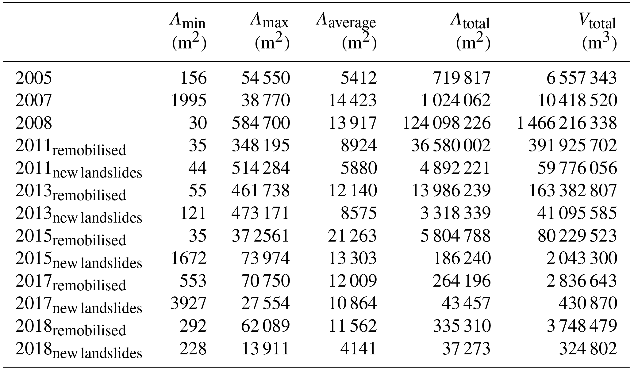
The number of coseismic deposits that were remobilised in each period, the area affected by the remobilisation and the number and areas of new failure (i.e. the post-seismic landslides) decreased significantly over time (Table 3). The coseismic landslides covered 124 km2; only 37 km2 had some activity (A1–A3) in 2011, while only 14 km2 was active in 2013, 6 km2 in 2015, 0.27 km2 in 2017 and 0.34 km2 in 2018. Furthermore, the degree of activity of the coseismic deposits rapidly decreased and, with time, the number and areas of active slides decayed faster than that of debris flows. A great number of remobilisations in the form of debris flows were identified within the first 3 years after the earthquake (2008–2011). Then (2013–2018), the number of debris flows decreased considerably, although a large amount of coseismic material was still present on the hillslopes (Fan et al., 2018a). This suggests that the effects of the earthquake on landslide rates might be smaller than what was initially expected (Huang and Fan, 2013). Some ongoing studies suggest that the changing properties of the coseismic deposits, such as in terms of grain size distribution, relative density and hydraulic conductivity, might play a key role.
Table 3Simple statistics of the landslides included in the multi-temporal inventory. Note that the volumes in this table were calculated according to the area–volume scaling proposed by Xu et al. (2016). Amin, Amax, Aaverage, Atotal and Vtotal are, respectively, the minimum, maximum, average and total area of landslides and their estimated total volume.
The frequency-size distribution analysis (e.g. Malamud et al., 2004) carried out with the dataset (Fig. 8) shows the patterns of pre- and coseismic landslides and post-seismic remobilisations for the period 2005–2018. The largest number of landslides was triggered by the earthquake, while the post-seismic rates of remobilisation decreased over the following years. This decrease mostly occurred for landslides with small areas, while the curves do not exhibit important changes in the range of landslides with a large area (A>105 m2). The shifting of the roll-over point towards higher landslide areas over time might indicate that the minimum sampling size (Malamud et al., 2004; Guzzetti et al., 2002) or the minimum area that can fail due to physical reasons (Turcotte et al., 2002) is increasing over time.
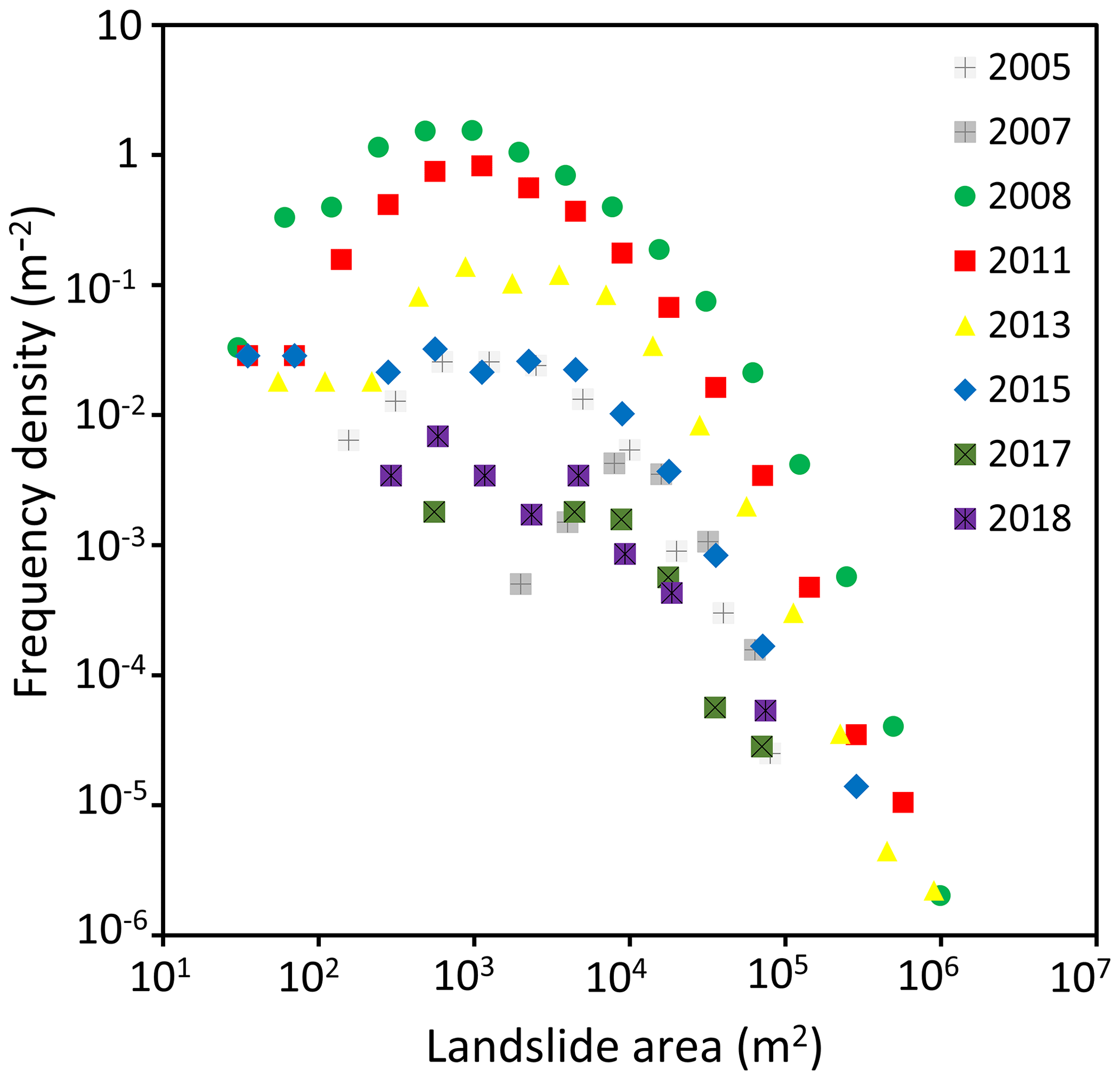
Figure 8Frequency density–size distributions of pre-seismic landslides (2005–2007), coseismic landslides (2008) and post-seismic remobilisations (2011–2018) in the landslide inventory. Note that the amount of data in 2007, 2017 and 2018 might be insufficient to delineate clear patterns and identify a roll-over point.
3.1.4 Comparison with existing inventories
Approaches used to compare landslide inventory maps can entail direct or indirect comparisons (Gorum et al., 2011). The former evaluate the degree of cartographic matching between two maps through a pairwise comparison (e.g. Galli et al., 2008), while the latter correlate the inventories through the landslide densities (e.g. Guzzetti et al., 2000), frequency–area statistics (e.g. Galli et al., 2008) or the resulting susceptibility or hazard maps (e.g. van Westen et al., 2009). Here we provide direct and indirect comparisons between our coseismic inventory and the portions of those presented by Dai et al. (2011), Xu et al. (2014) and Tang et al. (2016) that overlap with it.
The matching degrees (M; see Eq. 1) show a wide range. The worst overall match is with the Dai et al. (2011) inventory, with M=0.32. The match with the inventory by Xu et al. (2014) is 0.47, while the best match (M=0.82) is obtained with the inventory by Tang et al. (2016). Note that this matching degree is comparable to those obtained between the different mappers that produced our inventory. Through visual comparison, we can see that Dai et al. (2011) identified fewer landslides in our study area than we did. This might be partly explained by the lower aerial coverage of the images they used, compared to those we used. The images used by Xu et al. (2014) had comparable coverage to those we used. They identified a similar number of landslides in our study area. The mismatch with our inventory could be due to different criteria used in mapping. The matching degree has also been calculated for the other inventories. In such a case, the variability is smaller, as it ranges from 0.33 to 0.44. Tang et al. (2016) vs. Xu et al. (2014) show a higher correlation (M=0.44) and Dai et al. (2011) vs. Xu et al. (2014), and Tang et al. (2016) vs. Dai et al. (2011) 0.34 show the lowest, at M=0.33 and 0.34, respectively. These results suggest that our inventory and the one by Tang et al. (2016) are the most similar, and the one that presents the poorest correlation with the others is by Dai et al. (2011).
Table 4Matching degrees, calculated for each of the catchments delineated in our study area, between our coseismic inventory and those of Tang et al. (2016), Dai et al. (2011) and Xu et al. (2014). The catchment areas and the areas of landslides are also reported. See Fig. 2 for the CID.
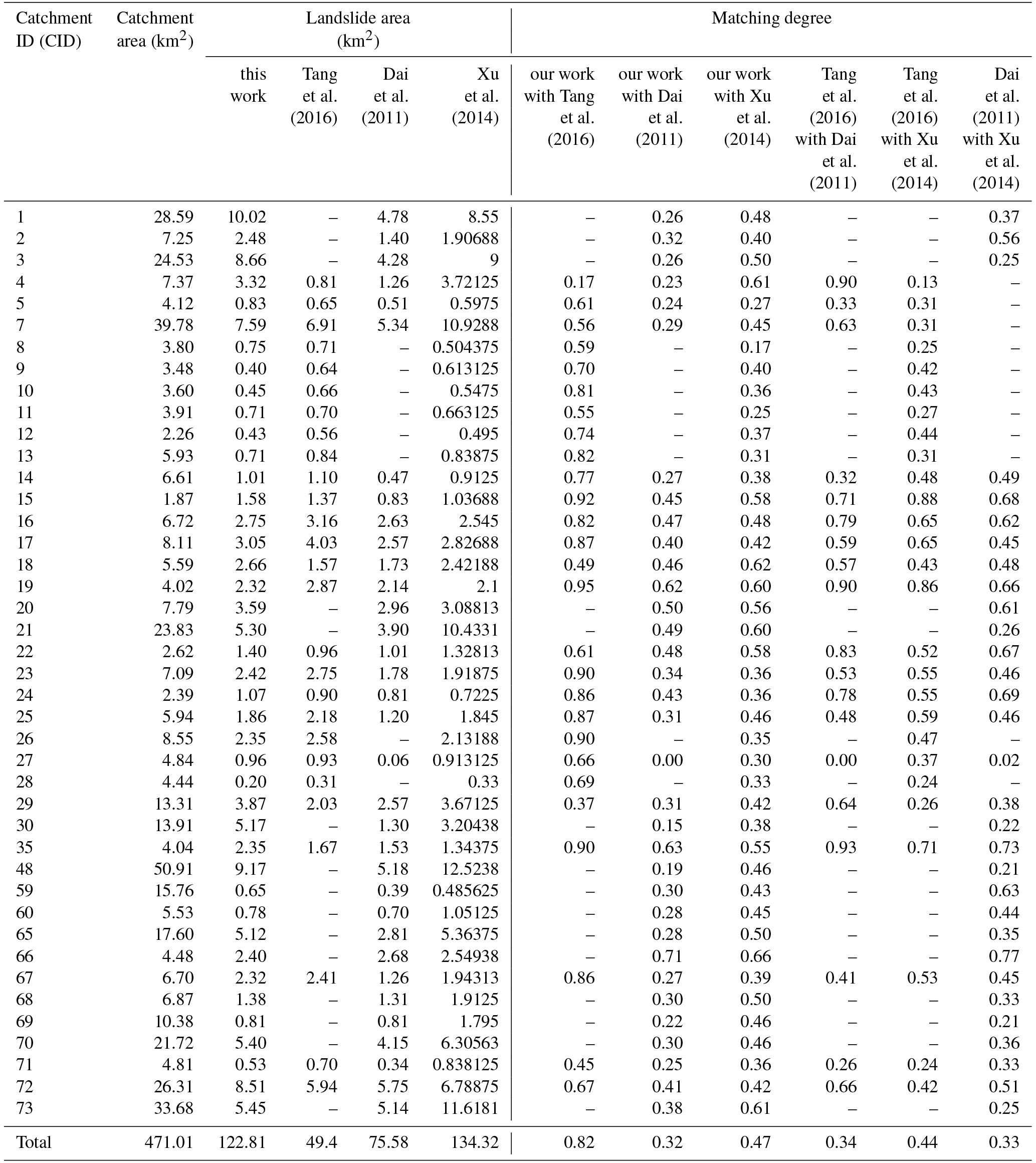
In order to verify the spatial variability of the matching degree, we repeated the analysis on the catchment scale, as reported in Table 4. The missing data for Tang et al. (2016) refer to those catchments that were not covered by their inventory. The results show that our inventory and that of Tang et al. (2016) are consistently similar in the areas in which they overlap, while the matching is much less spatially consistent with respect to the Dai et al. (2011) and Xu et al. (2014) inventories.
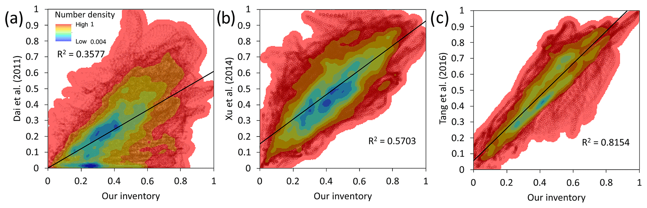
Figure 9Pixel-based spatial correlation of landslide densities. The comparisons between our inventory map and those obtained by Dai et al. (2011) (a), Xu et al. (2014) (b) and Tang et al. (2016) (c) are shown.
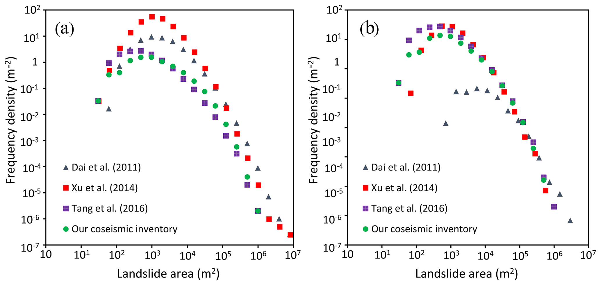
Figure 10Comparison of the frequency density – size distributions of the coseismic landslides mapped in the Wenchuan earthquake-affected area by Dai et al. (2011), Xu et al. (2014) and Tang et al. (2016). The relationship refers to the whole extension of each inventory in (a) and is limited to the area which is common to all the inventories in (b), i.e. the area mapped by Tang et al. (2016).
The comparison between the landslide density distributions yields the best correlation (R2=0.8154) with the inventory by Tang et al. (2016). Conversely, the lowest correlation is obtained with the Dai et al. (2011) inventory. This agrees with the result of the direct comparisons made through the matching degree.
Finally, in Fig. 10 we compare the frequency-density–size distributions of the four inventories. First, we compare the results referring to the entire areas covered by each inventory (Fig. 10a). The Dai et al. (2011) and Xu et al. (2014) inventories exhibit higher peak values of landslide density. This can depend on the extension of the mapped area, which can include or exclude areas with little or no landsliding. It also can be noted that the roll-over points of Dai et al. (2011) and Xu et al. (2014) inventories occur in correspondence to larger landslide areas than in our inventory and that of Tang et al. (2016). This can be in part explained by the predominantly small size of the landslides in our study area compared to those of other portions of the earthquake-affected region, and in part by a possible systematic undersampling of small landslides in Dai et al. (2011) and Xu et al. (2014). Undersampling seems particularly striking in Dai et al. (2011) when the same mapped area is used as the base of the comparison (Fig. 10b). To a lesser extent, it can be seen also in Xu et al. (2011) for small landslide areas (less than a few hundred m2). Our inventory and that of Tang et al. (2016) seem to suffer from undersampling with the same (possibly minimal) extent. Note also that Dai et al. (2011) show oversampling for large landslide areas, which might signal some systematic amalgamation of smaller landslide polygons.
For further comparison, we estimated the volume of the coseismic landslides through a set of empirical area–volume scaling relationships from the literature (Guzzetti et al., 2009; Larsen et al., 2010; Parker et al., 2011; Xu et al., 2016). These relationships provide a quick, first-order estimation of the landslide volumes from the mapped landslide areas. They were calibrated by their authors in different ways (i.e. using landslide depths measured in the field or differential DEM techniques on datasets of different sizes). Guzzetti et al. (2009) calibrated their relationship using data from 677 landslides of the slide type, with areas ranging from 2 to 109 m2; Larsen et al. (2010) employed a dataset of 4231 landslides, comprising soil and bedrock failures ranging from 1 to 107 m2; Parker et al. (2011) used field measurements of 41 coseismic landslides triggered by the 2008 Wenchuan earthquake but they did not provide information on the sizes of these landslides; Xu et al. (2016) used both field observations and remote-sensing analyses of 1415 coseismic landslides triggered by the 2008 Wenchuan earthquake, all having sizes exceeding 104 m2.
Table 5Comparison between the total volumes of coseismic landslides in the portion of the Wenchuan earthquake-affected area that was covered by all the inventories (i.e. our inventory and those of Dai et al., 2011; Xu et al., 2014; Tang et al. 2016), estimated through area–volume empirical relationships (Guzzetti et al., 2009; Larsen et al., 2010; Parker et al., 2011; Xu et al., 2016). The first value in each cell is the central value, while those in brackets result from the uncertainty (±1σ) of the calibrated parameters of the relationships.
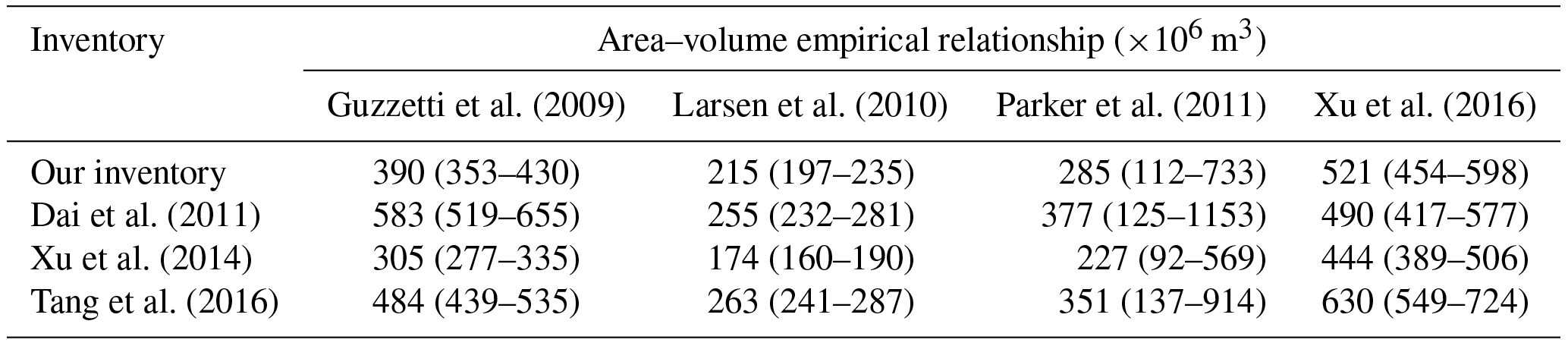
Table 6Structure of the dataset of debris flows and their triggering rainfalls. An additional shape file is provided to define the catchment boundaries with a simple characterisation (CID, catchment name and county, gradient and internal relief, drainage density and channel length).

Attributes: DF_ID is the identifier of the debris flow, CID is the identifier of the catchment to which the debris flow or the rain gauge belong, Gully_name is the name of the catchment, latitude is the latitude of the debris flow event (∘), longitude is the longitude of the debris flow event (∘), year is the year the debris flow event occurred, month is the month the debris flow event occurred, day is the day the debris flow event occurred, Time_24h_ is the time at which the debris flow occurred (24 h), T_Comment is specifications on the time of occurrence of the debris flow (initiation, deposition or range of days), Source_vol is available material during the initiation of the debris flow (m3), Depo_vol is the volume of debris flow deposited at the fan area (m3), list_of_RG is the list of rain gauges (identifier) located in proximity to the debris flow event that were actively recording throughout the time window of interest for that debris flow, monitoring specifies whether additional monitoring data are available for that event (Y is yes; N is no), number of dams specifies the number of dams built in each catchment as mitigation measures, and references are the source of each debris flow event. * One folder for each debris flow event is X, the debris flow event identifier (DF_ID). Each folder contains the rain gauges located within a distance of 5 km for a given event. A indicates the relative position of each rain gauge from the debris flow event in ascending order; B refers to the rain gauge identifier (RG_ID); C, D and E indicate the year, month and day of the debris flow event, and F refers to the starting time of the rain. Rain is expressed in millimetres. Each spreadsheet provides data from 7 days before to 1 day after the date associated with the debris flow event (DF_ID). Full data series are available from the authors upon request for further analysis.
These empirical relationships are expressed using a power law in the form: , where V is the individual landslide volume, A is the mapped individual landslide area, and α and γ are calibrated parameters. A higher value of γ underlies an abundance of deep bedrock landslides in the calibration dataset, while lower values of γ are more representative of shallow landslides, as discussed by Parker et al. (2011). The relationships, with the uncertainties (±1σ) in the calibrated parameters, as given by the respective authors, read as follows: (Guzzetti et al., 2009), (Larsen et al., 2010), (Parker et al., 2011), and (Xu et al., 2016).
The total landslide volume is, obviously, the sum of the individually computed landslide volumes. As noted by Parker et al. (2011), if the inventory includes amalgamated landslide polygons, there will be a systematic overestimation of the total volume. For our mapping we are confident, also in the light of the comparisons presented in Fig. 10, that the incidence of amalgamation is limited, as the polygon-based mapping was performed by visual interpretation with field-checking on high-resolution images, rather than by semi-automatic mapping techniques, which have been shown to be more susceptible to this kind of mapping error (e.g. Marc and Hovius, 2005). The results of the calculations using the various empirical relations applied to the landslide polygons (total areas of landslide, without differentiation between source, track and deposition areas) mapped in various inventories are reported in Table 5, with reference to the region that is covered by all the inventories (which corresponds to the region mapped by Tang et al., 2016). Note that the relationship by Larsen et al. (2010) consistently yields the smallest volumes for all the inventories, while the largest volumes are obtained either through Guzzetti et al. (2009) or Xu et al. (2016) relationships, depending on the inventory. Also note that, in the given study area, depending on the inventory map and the scaling relationship, volumes in a wide range (174–630×106 m3) can be estimated, to which the uncertainties in the scaling parameters and on the landslide boundaries also should be added. If the former are considered (in the form of ±1σ; see Table 5), the volume range will span over 1 order of magnitude (92–1153×106 m3). Quantifying the latter is more difficult, but has been attempted for our inventory (see Sect. 3.1.2, Fig. 7, and Fan et al., 2018a).
Table 7Released information on some well-monitored catchments.
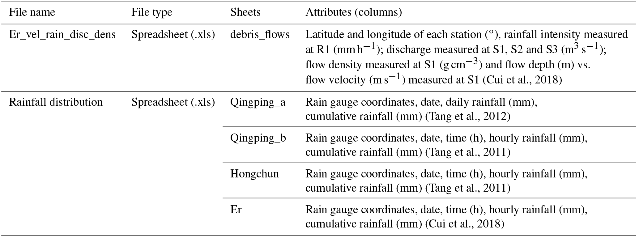
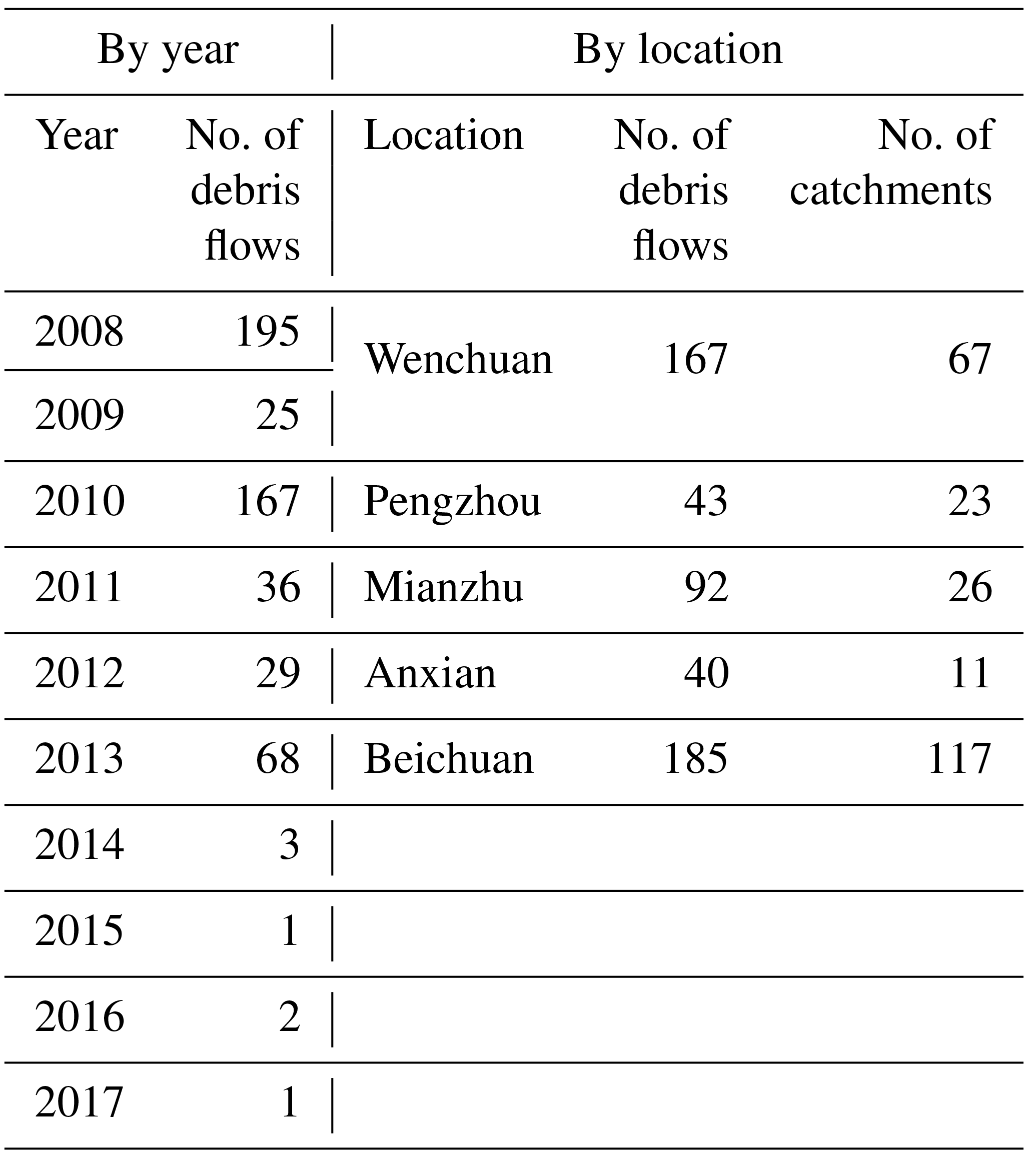
Table 8Simple statistics of the debris flows and their triggering rainfalls recorded in the dataset.
3.2 Inventory of debris flows and their triggering rainfalls
3.2.1 Data acquisition, structure of the dataset and attributes
We compiled a dataset of debris flows from the existing literature which occurred after the 2008 Wenchuan earthquake until the rainy season in summer 2017. These events are associated with the recordings of rain gauges and are spread over an area of 16 959 km2.
The structure of the dataset is summarised in Table 6. The dataset contains information on the locations, date and time of occurrence of debris flows and on the rainfall that triggered them. We included data not only for catastrophic and well-studied events (e.g. Tang et al., 2012; Xu et al., 2012), but also for smaller events that did not cause fatalities or heavy damage to the population and the infrastructure, but had sufficient run-out to approach or reach the catchment outlet. The material of these events can come from different slides, hillslope and channelised debris flows and, mainly, from the existing channel deposits, all of them presented in the multi-temporal inventory of landslides (Sect. 2.1 and 3.1). We used a 25 m resolution digital elevation model, provided by the Sichuan Bureau of Surveying and Mapping, to define the catchment boundaries. The rainfall data were obtained from the Meteorological Administration of China, from the Meteorological Bureau of Sichuan Province, from the bureau of land and resources of Chengdu and from the WebGIS monitoring network of the State Key Laboratory of Geohazard Prevention and Geoenvironment Protection (SKLGP, Chengdu, China; see Huang et al., 2015). These data were all recorded with automatic rain gauges.
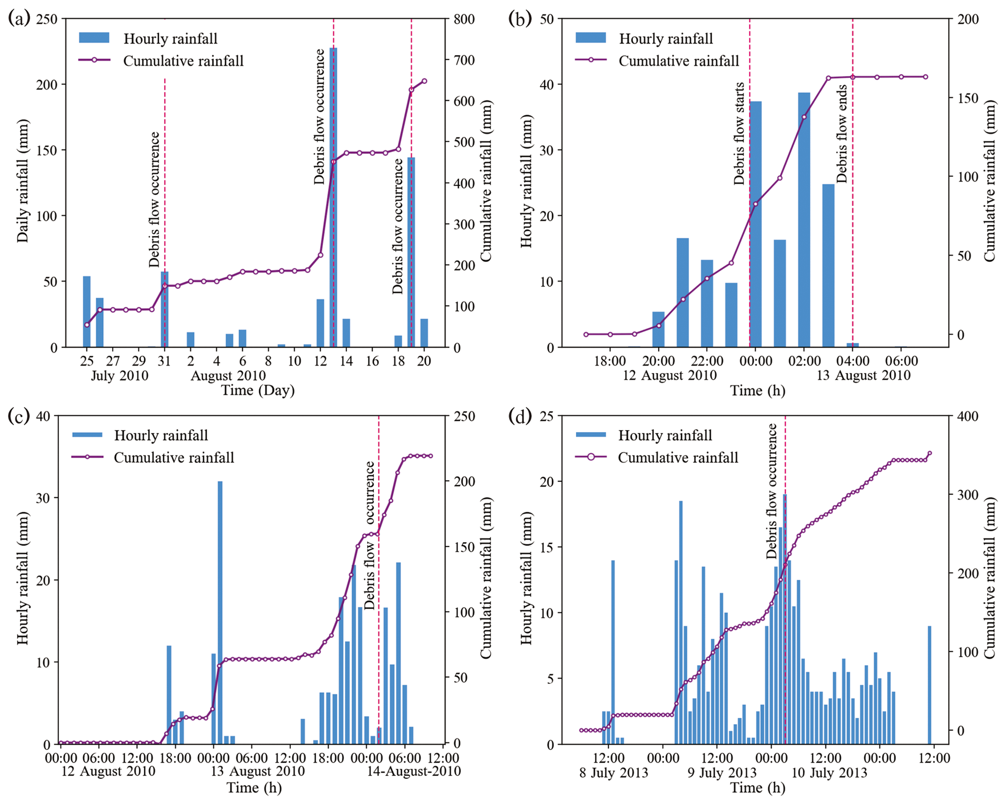
Figure 11(a) Daily and accumulated precipitation in Qingping (Wenjia gully, CID M9, Mianzhu County; no. 4 in Fig. 1c) during a period affected by the three debris flow events. The DF_ID of these events are, chronologically, 272, 302 and 273. Rainfall data were recorded by a rain gauge located in Nanmu (CID M22, lat 104.154533, long 31.48832, Yu et al., 2010). (b) Detail of the second debris flow (DF_ID 302) that occurred between 12 and 13 August 2010 in Qingping: hourly and accumulated precipitations and event start and end are represented. (c) Hourly and accumulated precipitation in Hongchun (CID W25, Wenchuan County; no. 2 in Fig. 1c). A debris flow occurred on 14 August 2010 (DF_ID 53). Rainfall data were recorded by a rainfall gauge located in Yingxiu (lat 103.4826, long 31.06417). (d) Hourly and accumulated precipitation in Er (CID W7, Wenchuan County; no. 1 in Fig. 1c). A debris flow occurred on 10 July 2013 (DF_ID 164). Rainfall data were recorded by a rainfall gauge located in Er (lat 103.46088, long 31.11679; R1 in Fig. 13a; Cui et al., 2018).
We verified most of the debris flows included in the dataset by reviewing 76 published works (see file named “References of data sources” in the repository). For the largest and most catastrophic events, we carried out field investigations and interviews with the local residents with a minimum of two surveyors. There is no fixed period of the year during which field inspections were carried out, as they mostly followed the occurrence of strong rainfall. We also collected information from the monitoring system that the SKLGP implemented in some catchments (see Fig. 1). The debris flows were geo-referenced through the latitude and longitude of the outlet of the catchment in which they occurred. Information on the rainfall that triggered each debris flow is provided for the rain gauges located in closest proximity to them (<5 km). In case no rain gauges were actively recording within this distance, data from the closest rain gauge are provided. There are 391 of 527 debris flow-affected catchments with rain gauges within 5 km from the locations of the catchment outlets. We chose to provide rainfall data with the highest resolution available (in most cases hourly rainfall, in some cases 10 min rainfall) for a time window starting from 1 week before to 1 day after the debris flow event. The choice of this window should allow for the inclusion of the significant antecedent rainfall in our setting that can be used for further analyses of the triggering conditions of the debris flows. If the reader requires them, rainfall series with wider time windows can be obtained from the authors upon request.
For one catchment (Er catchment; no. 1 in Fig. 1b; Table 7; Cui et al., 2018), we release data series of rainfall intensity, flow discharge, density and height. The Er catchment is administratively part of Yingxiu township and covers 39.4 km2 with a channel length of 11.5 km. The Ergou River flows within the catchment, which is a tributary of the Minjiang River. The headwater elevation of the catchments is 4120 m a.s.l. and the outlet is located at 990 m a.s.l. Rainfall intensity was obtained through rain gauges with 0.5 mm tipping buckets. Flow discharge was calculated as the product of the cross-sectional mean velocity and the cross-sectional area of the flow. The latter was calculated from the depth, obtained from the data measured by the ultrasonic stage meter, in combination with the detailed geometry of each section. The surface velocity of the flow was measured using automatic radar speed indicators and compared with video images (Yan et al., 2016). As flow velocity varies with depth, the relationship obtained by Takahashi (1991) was used. Flow depths were measured using ultrasonic stage meters TSS908, Beijing Guda instrument Co., Ltd.), with 1 min recording frequency, 0–30 m measurement range and ±10 mm error. For additional information, the reader is referred to Cui et al. (2018). For other well-monitored catchments (nos. 2, 3 and 4 in Fig. 1b), we release rainfall data for three important debris flow events (see Sect. 3.2.3, below), while full data series are available from the authors upon request.
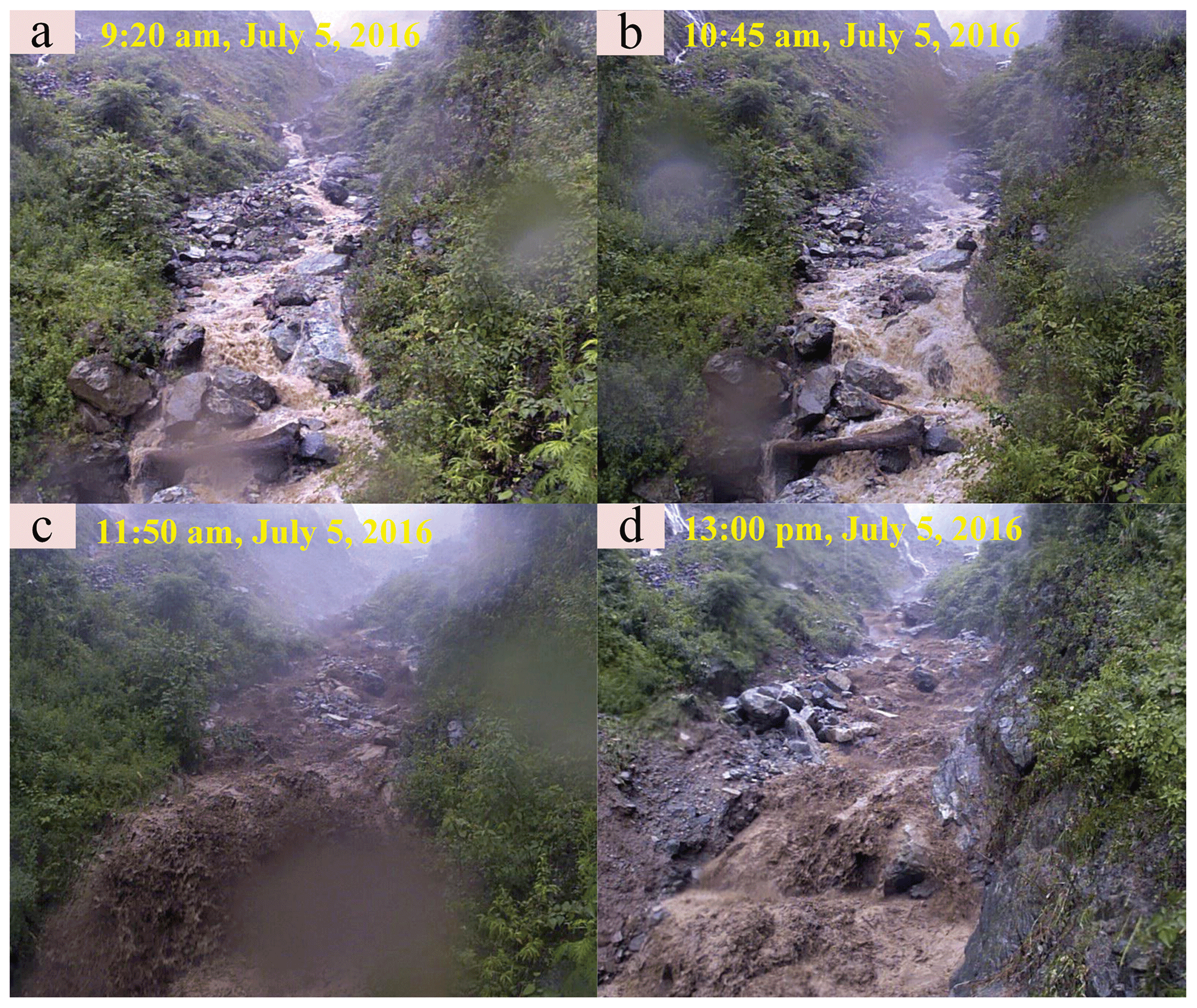
Figure 12Debris flow event recorded in Er (CID W7, Wenchuan County; no. 1 in Fig. 1c) on 5 July 2016 (Cui et al., 2018).
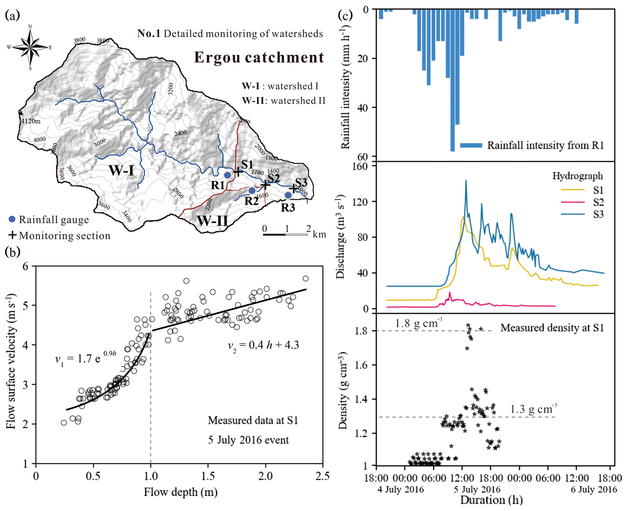
Figure 13Data analysis of the debris flow which occurred on 5 July 2016 (Fig. 12) in Er (CID W7, Wenchuan County; no. 1 in Fig. 1c; Cui et al., 2018). (a) Map of the catchment, (b) flow surface velocity vs. flow depth, and (c) rainfall intensity, flow discharge and flow density.
3.2.2 Uncertainties
Especially for minor debris flows, the time of debris flow occurrence may be uncertain, especially in those locations that lack proper instrumentation or eyewitnesses. Moreover, ambiguities in the definition of this time may occur, as the debris flow has a finite duration. In this work, the time refers to the arrival of the flow at the outlet of the catchment, unless otherwise stated.
Rainfall recordings from rain gauges located within or near a catchment in which a debris flow developed are not equally representative of the rainfall that actually triggered the debris flow and permitted its run-out. In our dataset we decided to be inclusive by using a wide buffer around the event location, so as not to discard some data series that may be useful for analyses of rainfall variability on a local scale and to perform interpolations. However, it is worth remembering that the spatio-temporal patterns of rainfall in mountainous areas can be extremely inhomogeneous (e.g. Nikolopoulos et al., 2014). Significant variations may exist even within the same catchment, over distances of a few kilometres or even just a few hundreds of metres (e.g. Smith et al., 2003; Panziera et al., 2011), in dependence, for instance, on the variability of the elevation, slope and aspect of the area, in combination with the local pattern of wind at the time of the rain event. Moreover, rain gauges are usually installed in valleys and channels, while debris flows originate high on the slopes (Stoffel et al., 2011), which can generate a systematic bias. The uncertainties that derive from imperfect choices of the representative rain gauge(s) for a debris flow event have been shown to lead to large underestimations of the debris flow-triggering thresholds and to strongly limit the performance of warning systems (Nikolopoulos et al., 2014; Guo et al., 2016, 2017). Therefore, these uncertainties should be carefully estimated and minimised with appropriate strategies whenever possible. Various studies, for instance, suggested the use of weather radar and satellite-based rainfall estimates to assess the representative rainfalls for debris flows (Kirschbaum et al., 2012; Rossi et al., 2012), but literature featuring methods to address the issue of rainfall variability systematically is still scarce (Guzzetti et al., 2007; Jakob et al., 2012).
3.2.3 Descriptive statistics
The dataset contains information about 527 debris flows which occurred in 244 catchments, and rainfall data from 91 rain gauges. Most of the debris flows occurred during the summertime heavy rainfalls of 2008, 2010 and 2013, particularly in the counties of Wenchuan and Beichuan (Table 8).
In Fig. 11, examples of rainfall data series are reported for well-monitored debris flow events in Qingping, Hongchun and Er catchments (see Table 7). In Figs. 12 and 13, the well-monitored debris flow event in Er catchment is shown (photographs, rainfall data, flow discharge, height and density).
The datasets are freely downloadable from https://doi.org/10.5281/zenodo.1405489 (Domènech et al., 2018). In addition to the data, the repository contains supplementary material (metadata files) that clarify the structures of the datasets, and a reference list for the data sources.
We presented a multi-temporal inventory of landslides in a portion of the area affected by the 2008 Wenchuan earthquake covering the period from 2005 to 2018 and an inventory of debris flows and their triggering rainfalls over a larger area covering the period from 2008 to 2017. The two datasets, which are freely available, can provide an insight into the spatial and temporal patterns of the enhanced mass wasting caused by a strong earthquake. We encourage other researchers to follow our example by sharing analogous datasets, so we can build an open collection of data and facilitate meta-analyses among multi-temporal datasets of mass wasting induced by earthquakes or other triggers.
XF designed the work together with GD and GS; GS wrote the manuscript; GD, LD and FY compiled the datasets and prepared the display items; GD, LD, and FY performed the mapping supervised by XF; XG and CH provided some of the data, and suggestions on some methods; XF, RH and QX acquired project funds and supervised the project; all authors revised and approved the datasets and the manuscript.
The authors declare that they have no conflict of interest.
The collection and processing of the data presented in this paper were funded
by the National Science Fund for Excellent Young Scholars of China (grant
no. 41622206), the Funds for Creative Research Groups of China (grant
no. 41521002), the Fund for International Cooperation (NSFC-RCUK_NERC),
Resilience to Earthquake-induced landslide risk in China (grant
no. 41661134010). We also want to thank the contribution of all the
experts in the group during the mapping.
Edited by: Giulio G. R. Iovine
Reviewed by: Alexander Strom, Theo W. J. van Asch, Tolga Gorum, and one
anonymous referee
Broeckx, J., Vanmaercke, M., Duchateau, R., and Poesen, J.: A data-based landslide susceptibility map of Africa, Earth-Sci. Rev., 185, 102–121, https://doi.org/10.1016/j.earscirev.2018.05.002, 2018.
Corominas, J., van Westen, C., Frattini, P., Cascini, L., Malet, J. P., Fotopoulou, S., Catani, F., Van Den Eeckhaut, M., Mavrouli, O., Agliardi, F., Pitilakis, K., Winter, M. G., Pastor, M., Ferlisi, S., Tofani, V., Hervás, J., and Smith, J. T.: Recommendations for the quantitative analysis of landslide risk, B. Eng. Geol. Environ., 73, 209–263, 2014.
Cui, P., Wei, F. Q., He, S. M., You, Y., Chen, X. Q., Li, Z. L., and Yang, C.L.: Mountain disasters induced by the earthquake of May 12 in Wenchuan and the disasters mitigation, J. Mt. Sci., 26, 280–282, 2008.
Cui, P., Chen, X. Q., Zhu, Y. Y., Su, F. H., Wei, F. Q., Han, Y. S., Liu, H. J., and Zhuang, J. Q.: The Wenchuan Earthquake (May 12, 2008), Sichuan Province, China, and resulting geohazards, Nat. Hazards, 56, 19–36, https://doi.org/10.1007/s11069-009-9392-1, 2011.
Cui, P., Guo, X., Yan, Y., Li, Y., and Ge, Y.: Real-time observation of an active debris flow watershed in the Wenchuan Earthquake area, Geomorphology, 321, 153–166 https://doi.org/10.1016/j.geomorph.2018.08.024, 2018.
Dadson, S. J., Hovius, N., Chen, H., Dade, W. B., Lin, J. C., Hsu, M. L., Lin, C. W., Horng, M. J., Chen, T. C., Milliman, J., and Stark, C. P.: Earthquake-triggered increase in sediment delivery from an active mountain belt, Geology, 32, 733–736, https://doi.org/10.1130/G20639.1, 2004.
Dai, F. C., Xu, X., Yao, X., Xu, L., Tu, X. B., and Gong, Q. M.: Spatial distribution of landslides triggered by the 2008 Ms 8.0 Wenchuan earthquake, China, J. Asian. Earth Sci., 40, 883–895, https://doi.org/10.1016/j.jseaes.2010.04.010, 2011.
Ding, H., Li, Y., Ni, S., Ma, G., Shi, Z., Zhao, G., Yan, L., and Yan, Z.: Increased sediment discharge driven by heavy rainfall after Wenchuan earthquake: A case study in the upper reaches of the Min River, Sichuan, China, Quatern. Int., 333, 122–129, https://doi.org/10.1016/j.quaint.2014.01.019, 2014.
Domènech, G., Yang, F., Guo, X., Fan, X., Scaringi, G., Dai, L., He, C., Xu, Q., and Huang, R.: Two multi-temporal datasets to track the enhanced landsliding after the 2008 Wenchuan earthquake, version 2, Zenodo, https://doi.org/10.5281/zenodo.1405489, 2018.
Đurić, D., Mladenović, A., Pešić-Georgiadis, M., Marianović, M., and Abolmasov, B.: Using multiresolution and multitemporal satellite data for post-disaster landslide inventory in the Republic of Serbia, Landslides, 14, 1467–1482, https://doi.org/10.1007/s10346-017-0847-2, 2017.
Fan, X., van Westen, C. J., Korup, O., Görüm, T., Xu, Q., Dai, F., Huang, R., and Wang, G.: Transient water and sediment storage of the decaying landslide dams induced by the 2008 Wenchuan earthquake, China, Geomorphology, 171–172, 58–68, https://doi.org/10.1016/j.geomorph.2012.05.003, 2012.
Fan, X., Xu, Q., Scaringi, G., Dai, L., Li, W., Dong, X., Zhu, X., Pei, X., Dai, K., and Havenith, H. B.: Failure mechanism and kinematics of the deadly June 24th 2017 Xinmo landslide, Maoxian, Sichuan, China, Landslides, 14, 2129–2146, https://doi.org/10.1007/s10346-017-0907-7, 2017a.
Fan, X., Xu, Q., van Westen, C. J., Huang, R., and Tang, R.: Characteristics and classification of landslide dams associated with the 2008 Wenchuan earthquake, Geoenvironmental Disasters, 4, 12, https://doi.org/10.1186/s40677-017-0079-8, 2017b.
Fan, X., Domènech, G., Scaringi, G., Huang, R., Xu, Q., Hales, T. C., Dai, L., Yang, Q., and Francis, O.: Spatio-temporal evolution of mass wasting after the 2008 Mw 7.9 Wenchuan Earthquake revealed by a detailed multi-temporal inventory, Landslides, 15, 2325–2341, https://doi.org/10.1007/s10346-018-1054-5, 2018a.
Fan, X., Juang, C. H., Wasowski, J., Huang, R., Xu, Q., Scaringi, G., van Westen, C. J., and Havenith, H. B.: What we have learned from the 2008 Wenchuan Earthquake and its aftermath: A decade of research and challenges, Eng. Geol., 241, 25–32, https://doi.org/10.1016/j.enggeo.2018.05.004, 2018b.
Fan, X., Scaringi, G., Xu, Q., Zhan, W., Dai, L., Li, Y., Pei, X., Yang, Q., and Huang, R.: Coseismic landslides triggered by the 8th August 2017 Ms 7.0 Jiuzhaigou earthquake (Sichuan, China): factors controlling their spatial distribution and implications for the seismogenic blind fault identification, Landslides, 15, 967–983, https://doi.org/10.1007/s10346-018-0960-x, 2018c.
Fan, X., Xu, Q., and Scaringi, G.: Brief communication: Post-seismic landslides, the tough lesson of a catastrophe, Nat. Hazards Earth Syst. Sci., 18, 397–403, https://doi.org/10.5194/nhess-18-397-2018, 2018d.
Galli, M., Ardizzone, F., Cardinali, M., Guzzetti, F., and Reichenbach, P.: Comparing landslide inventory maps, Geomorphology, 94, 268–289, https://doi.org/10.1016/j.geomorph.2006.09.023, 2008.
Gariano, S. L. and Guzzetti, F.: Landslides in a changing climate, Earth-Sci. Rev., 162, 227–252, https://doi.org/10.1016/j.earscirev.2016.08.011, 2016.
Gorum, T., Fan, X., van Westen, C. J., Huang, R., Xu, Q., Tang, C., and Wang G.: Distribution pattern of earthquake-induced landslides triggered by the 12 May 2008 Wenchuan earthquake, Geomorphology, 133, 152–167, https://doi.org/10.1016/j.geomorph.2010.12.030, 2011.
Guo, X., Cui, P., Li, Y., Ma, L., Ge, Y., and Mahoney, W. B.: Intensity-duration threshold of rainfall-triggered debris flows in the Wenchuan Earthquake affected area, China, Geomorphology, 253, 208–216, https://doi.org/10.1016/j.geomorph.2015.10.009, 2016.
Guo, X., Cui, P., Marchi, L., and Ge, Y.: Characteristics of rainfall responsible for debris flows in Wenchuan Earthquake area, Environ. Earth Sci., 76, 596, https://doi.org/10.1007/s12665-017-6940-y, 2017.
Guzzetti, F., Malamud, B. D., Turcotte, D. L., and Reichenbach, P.: Power-law correlations of landslide areas in Central Italy, Earth Planet. Sc. Lett., 195, 169–183, https://doi.org/10.1016/S0012-821X(01)00589-1, 2002.
Guzzetti, F., Peruccacci, S., Rossi, M., and Stark, C. P.: Rainfall thresholds for the initiation of landslides in central and southern Europe, Meteorol. Atmos. phys., 98, 239–267, https://doi.org/10.1007/s00703-007-0262-7, 2007.
Guzzetti, F., Ardizzone, F., Cardinali, M., Rossi, M., and Valigi, D.: Landslide volumes and landslide mobilization rates in Umbria, central Italy, Earth Planet. Sc. Lett, 279, 222–229, https://doi.org/10.1016/j.epsl.2009.01.005, 2009.
Guzzetti, F., Mondini, A. C., Cardinali, M., Fiorucci, F., Santangelo, M., and Chang, K.-T.: Landslide inventory maps: New tools for an old problem, Earth-Sci. Rev., 112, 42–66, https://doi.org/10.1016/j.earscirev.2012.02.001, 2012.
Harp, E. L., Keefer, D. K., Sato, H. P., and Yagi, H.: Landslide inventories: the essential part of seismic landslide hazard analyses, Eng. Geol., 122, 9–21, https://doi.org/10.1016/j.enggeo.2010.06.013, 2011.
Hovius, N., Meunier, P., and Ching-weei, L.: Prolonged seismically induced erosion and the mass balance of a large earthquake, Earth Planet. Sc. Lett., 304, 347–355, https://doi.org/10.1016/j.epsl.2011.02.005, 2011.
Hu, W., Scaringi, G., Xu, Q., Pei, G., van Asch, T. W. J., and Hicher, P. Y.: Sensitivity of the initiation and runout of flowslides in loose granular deposits to the content of small particles: An insight from flume tests, Eng. Geol., 231, 34-44, https://doi.org/10.1016/j.enggeo.2017.10.001, 2017.
Huang, J., Huang, R., Ju, N., Xu, Q., and He, C.: 3D WebGIS platform for debris flow early warning: A case study, Eng. Geol., 197, 57–66, https://doi.org/10.1016/j.enggeo.2015.08.013, 2015.
Huang, R. and Fan, X.: The landslide story, Nat. Geosci., 6, 325–326, https://doi.org/10.1038/ngeo1806, 2013.
Hungr, O., Leroueil, S., and Picarelli, L.: The Varnes classification of landslide types, an update, Landslides, 11, 167–194, https://doi.org/10.1007/s10346-013-0436-y, 2014.
Jakob, M., Owen, T., and Simpson, T.: A regional real-time debris flow warning system for the District of North Vancouver, Canada, Landslides, 9, 165–178, https://doi.org/10.1007/s10346-011-0282-8, 2012.
Kargel, J. S., Leonard, G. J., Shugar, D. H., Haritashya, U. K., Bevington, A., Fielding, E. J., Fujita, K., Geertsema, M., Miles, E. S., Steiner, J., Anderson, E., Bajracharya, S., Bawden, G. W., Breashears, D. F., Byers, A., Collins, B., Dhital, M. R., Donnellan, A., Evans, T. L., Geai, M. L., Glasscoe, M. T., Green, D., Gurung, D. R., Heijenk, R., Hilborn, A., Hudnut, K., Huyck, C., Immerzeel, W. W., Liming, J., Jibson, R., Kaab, A., Khanal, N. R., Kirschbaum, D., Kraaijenbrink, P. D. A., Lamsal, D., Shiyin, L., Mingyang, L., McKinney, D., Nahirnick, N. K., Zhuotong, N., Ojha, S., Olsenholler, J., Painter, T. H., Pleasants, M., Pratima, K. C., Yuan, Q. I., Raup, B. H., Regmi, D., Rounce, D. R., Sakai, A., Donghui, S., Shea, J. M., Shrestha, A. B., Shukla, A., Stumm, D., van der Kooij, M., Voss, K., Xin, W., Weihs, B., Wolfe, D., Lizong, W., Xiaojun, Y., Yoder, M. R., and Young, N. : Geomorphic and geologic controls of geohazards induced by Nepal's 2015 Gorkha earthquake, Science, 351, aac8353, https://doi.org/10.1126/science.aac8353, 2016.
Keefer, D. K.: Landslides caused by earthquakes, Geol. Soc. Am. Bull., 95, 406–421, https://doi.org/10.1130/0016-7606(1984)95<406:LCBE>2.0.CO, 1984.
Keefer, D. K.: The importance of earthquake-induced landslides to long-term slope erosion and slope-failure hazards in seismically active regions, Geomorphology, 10, 265–284, https://doi.org/10.1016/0169-555X(94)90021-3, 1994.
Keefer, D. K.: Investigating Landslides Caused by Earthquakes – A Historical Review, Surv. Geophys., 23, 473–510, https://doi.org/10.1023/A:1021274710840, 2002.
Kirschbaum, D., Adler, R., Hong, Y., Kumar, S., Peters-Lidard, C., and Lerner-Lam, A.: Advances in landslide nowcasting: evaluation of a global and regional modeling approach, Environ. Earth Sci., 66, 1683–1696, https://doi.org/10.1007/s12665-011-0990-3, 2012.
Koi, T., Hotta, N., Ishigaki, I., Matuzaki, N., Uchiyama, Y., and Suzuki, M.: Prolonged impact of earthquake-induced landslides on sediment yield in a mountain watershed: The Tanzawa region, Japan, Geomorphology, 101, 692–702, https://doi.org/10.1016/j.geomorph.2008.03.007, 2008.
Larsen, I. J., Montgomery, D. R., and Korup, O.: Landslide erosion controlled by hillslope material, Nat. Geosci., 3, 247–251, https://doi.org/10.1038/NGEO776, 2010.
Li, G., West, A. J., Densmore, A. L., Jin, Z., Parker, R. N., and Hilton, R. G.: Seismic Mountain building: Landslides associated with the 2008 Wenchuan earthquake in the context of a generalized model for earthquake volume balance, Geochem. Geophys. Geosyst., 15, 833–844, https://doi.org/10.1002/2013GC005067, 2014.
Li, G., West, A. J., Densmore, A. L., Jing, Z., Zhang, F., Wang, J., Clark, M., and Hilton, R. G.: Earthquakes drive focused denudation along a tectonically active mountain front, Earth Planet. Sc. Lett., 472, 253–265, https://doi.org/10.1016/j.epsl.2017.04.040, 2017.
Lin, C. W., Liu, S. H., Lee, S. Y., and Lu, C. C.: Impacts of the Chi-Chi earthquake on subsequent rainfall-induced landslides in central Taiwan, Eng. Geol., 86, 87–101, https://doi.org/10.1016/j.enggeo.2006.02.010, 2006.
Malamud, B. D., Turcotte, D. L., Guzzetti, F., and Reichenbach, P.: Landslide inventories and their statistical properties, Earth Surf. Proc. Land., 29, 687–711, 2014.
Marc, O. and Hovius, N.: Amalgamation in landslide maps: effects and automatic detection, Nat. Hazards Earth Syst. Sci., 15, 723–733, https://doi.org/10.5194/nhess-15-723-2015, 2015.
Marc, O., Hovius, N., Meunier, P., Uchida, T., and Hayashi, S.: Transient changes of landslide rates after earthquakes, Geology, 43, 883–886, https://doi.org/10.1130/G36961.1, 2015.
Marc, O., Hovius, N., and Meunier, P.: The mass balance of earthquakes and earthquake sequences, Geophys. Res. Lett., 43, 3708–3716, https://doi.org/10.1002/2016GL068333, 2016a.
Marc, O., Hovius, N., Meunier, P., Gorum, T., and Uchida, T.: A seismologically consistent expression for the total area and volume of earthquake-triggered landsliding, J. Geophys. Res.-Earth, 121, 640–663, https://doi.org/10.1002/2015JF003732, 2016b.
Marc, O., Meunier, P., and Hovius, N.: Prediction of the area affected by earthquake-induced landsliding based on seismological parameters, Nat. Hazards Earth Syst. Sci., 17, 1159–1175, https://doi.org/10.5194/nhess-17-1159-2017, 2017.
Meunier, P., Hovius, N., and Haines, J. A.: Topographic site effects and the location of earthquake induced landslides, Earth Planet. Sc. Lett. 275, 221–232, https://doi.org/10.1016/j.epsl.2008.07.020, 2008.
Nikolopoulos, E. I., Crema, S., Marchi, L., Marra, F., Guzzetti, F., and Borga, M.: Impact of uncertainty in rainfall estimation on the identification of rainfall thresholds for debris flow occurrence, Geomorphology, 221, 286–297, https://doi.org/10.1016/j.geomorph.2014.06.015, 2014.
Panziera, L., Germann, U., Gabella, M., and Mandapaka, P. V.: NORA–Nowcasting of Orographic Rainfall by means of Analogues, Q. J. Roy. Meteor. Soc., 137, 2106–2123, https://doi.org/10.1002/qj.878, 2011.
Parker, R. N., Densmore, A. L., Rosser, N. J., De Michele, M., Li, Y., Huang, R., Whadcoat, S., and Petley, D. N.: Mass wasting triggered by the 2008 Wenchuan earthquake is greater than orogenic growth, Nat. Geosci., 4, 449–452, https://doi.org/10.1038/ngeo1154, 2011.
Parker, R. N., Hancox, G. T., Petley, D. N., Massey, C. I., Densmore, A. L., and Rosser, N. J.: Spatial distributions of earthquake-induced landslides and hillslope preconditioning in the northwest South Island, New Zealand, Earth Surf. Dynam., 3, 501–525, https://doi.org/10.5194/esurf-3-501-2015, 2015.
Pawłuszek, K., Borkowski, A., and Tarolli, P.: Towards the optimal pixel size of DEM for automatic mapping of landslide areas, The International Archives of the Photogrammetry, Remote Sensing and Spatial Information Sciences, Vol. XLII-1/W1, 2017 ISPRS Hannover Workshop: HRIGI 17 – CMRT 17 – ISA 17 – EuroCOW 17, 6–9 June 2017, Hannover, Germany, https://doi.org/10.5194/isprs-archives-XLII-1-W1-83-2017, 2017.
Rodriguez, C. E., Bommer, J. J., and Chandler, R. J.: Earthquake-induced landslides: 1980–1997, Soil Dyn. Earthq. Eng., 18, 325–346, https://doi.org/10.1016/S0267-7261(99)00012-3, 1999.
Rossi, M., Kirschbaum, D., Luciani, S., Mondini, A. C., and Guzzetti, F.: TRMM satellite rainfall estimates for landslide early warning in Italy: preliminary results, P. SPIE, 8523, 85230D, https://doi.org/10.1117/12.979672, 2012.
Qi, S., Xu, Q., Lan, H., Zhang, B., and Liu, J.: Spatial distribution analysis of landslides triggered by 2008.5.12 Wenchuan Earthquake, China, Eng. Geol., 116, 95–108, https://doi.org/10.1016/j.enggeo.2010.07.011, 2010.
Santangelo, M., Marchesini, I., Bucci, F., Cardinali, M., Fiorucci, F., and Guzzetti, F.: An approach to reduce mapping errors in the production of landslide inventory maps, Nat. Hazards Earth Syst. Sci., 15, 2111–2126, https://doi.org/10.5194/nhess-15-2111-2015, 2015.
Scaringi, G., Fan, X., Xu, Q., Liu, C., Ouyang, C., Domènech, G., Yang, F., and Dai, L.: Some considerations on the use of numerical methods to simulate past landslides and possible new failures: the case of the recent Xinmo landslide (Sichuan, China), Landslides, 15, 1359–1375, https://doi.org/10.1007/s10346-018-0953-9, 2018.
Schmitt, R. G., Tanyas, H., Nowicki Jessee, M. A., Zhu, J., Biegel, K. M., Allstadt, K. E., Jibson, R. W., Thompson, E. M., van Westen, C. J., Sato, H. P., Wald, D. J., Godt, J. W., Görüm, T., Xu, C., Rathje, E. M., and Knudsen, K. L.: An open repository of earthquake-triggered ground-failure inventories, U.S. Geological Survey data release collection, https://doi.org/10.3133/ds1064, 2017.
Shieh, C. L., Chen, Y. S., Tsai, Y. J., and Wu, J. H.: Variability in rainfall threshold for debris flow after the Chi-Chi earthquake in central Taiwan, China, Int. J. Sediment. Res., 24, 177–188, https://doi.org/10.1016/S1001-6279(09)60025-1, 2009.
Smith, R. B., Jiang, Q., Fearon, M. G., Tabary, P., Dorninger, M., Doyle, J. D., and Benoit, R.: Orographic precipitation and air mass transformation: an Alpine example, Q. J. Roy. Meteor. Soc., 129, 433–454, https://doi.org/10.1256/qj.01.212, 2003.
Stoffel, M., Bollschweiler, M., and Beniston, M.: Rainfall characteristics for periglacial debris flows in the Swiss Alps: past incidences—potential future evolutions, Climatic Change, 105, 263–280, https://doi.org/10.1007/s10584-011-0036-6, 2011.
Takahashi, T.: Debris flow. Monograph of IAHR, AA Balkema, Rotterdam, 1991.
Tang, C., Zhu, J., Li, W. L., and Liang, J. T.: Rainfall-triggered debris flows following the Wenchuan earthquake, B. Eng. Geol. Environ., 68, 187–194, https://doi.org/10.1007/s10064-009-0201-6, 2009.
Tang, C., Zhu, J., Ding, J., Cui, X., Chen, L., and Zhang, J. S.: Catastrophic debris flows triggered by a 14 August 2010 rainfall at the epicenter of the Wenchuan earthquake, Landslides, 8, 485–497, https://doi.org/10.1007/s10346-011-0269-5, 2011.
Tang, C., van Asch, T.W J., Chang, M., Chen, G. Q., Zhao, X. H., and Huang, X. C.: Catastrophic debris flows on 13 august 2010 in the Qingping area, southwestern china: the combined effects of a strong earthquake and subsequent rainstorms, Geomorphology 139, 559–576, https://doi.org/10.1016/j.geomorph.2011.12.021, 2012.
Tang, C., Van Westen, C. J., Tanyas, H., and Jetten, V. G.: Analysing post-earthquake landslide activity using multi-temporal landslide inventories near the epicentral area of the 2008 Wenchuan earthquake, Nat. Hazards Earth Syst. Sci., 16, 2641–2655, https://doi.org/10.5194/nhess-16-2641-2016, 2016.
Tang, R., Fan, X., Scaringi, G., Xu, Q., van Westen, C. J., Ren, J., and Havenith, H. B.: Distinctive controls on the distribution of river-damming and non-damming landslides induced by the 2008 Wenchuan earthquake, B. Eng. Geol. Environ., https://doi.org/10.1007/s10064-018-1381-8, online first, 2018.
Tanyaş, H., van Westen, C. J., Allstadt, K. E., Nowicki Jessee, M. A., Görüm, T., Jibson, R. W., Godt, J. W., Sato, H. P., Schmitt, R. G., Marc, O., and Hovius, N.: Presentation and Analysis of a Worldwide Database of Earthquake-Induced Landslide Inventories, J. Geophys. Res.-Earth, 122, 1991–2015, https://doi.org/10.1002/2017JF004236, 2017.
Turcotte, D. L., Malamud, B. D., Guzzetti, F., and Reichenbach, P.: Self-organization, the cascade model, and natural hazards, P. Natl. Acad. Sci. USA, 19, 2530–2537, 2002.
van Westen, C. J., Seijmonsbergen, A. C., and Mantovani, F.: Comparing landslide hazard maps, Nat. Hazards, 20, 137–158, 1999.
van Westen, C. J., van Asch, T. W. J, and Soeters, R.: Landslide hazard and risk zonation—why is it still so difficult?, B. Eng. Geol. Environ., 65, 167–184, https://doi.org/10.1007/s10064-005-0023-0, 2006.
Wang, G., Huang, R., Lourenço, D. N., and Kamai, T.: A large landslide triggered by the 2008 Wenchuan (M8.0) earthquake in Donghekou area: Phenomena and mechanisms, Eng. Geol., 182, 148–157, https://doi.org/10.1016/j.enggeo.2014.07.013, 2014.
Wang, J., Jin, Z., Hilton, R. G., Zhang, F., Densmore, A. L., Li, G., and West, A. J.: Controls on fluvial evacuation of sediment from earthquake-triggered landslides, Geology, 43, 115–118, https://doi.org/10.1130/G36157.1, 2015.
Wang, W., Godard, V., Liu-Zeng, J., Scherler, D., Xu, C., Zhang, J., Xie, K., Bellier, O., Ansberque, C., de Sigoyer, J., and ASTER Team: Perturbation of fluvial sediments fluxes following the 2008 Wenchuan earthquake, Earth Surf. Proc. Land., 42, 2611–2622, https://doi.org/10.1002/esp.4210, 2017.
Xu, C., Xu, X., Yao, X., and Dai, F.: Three (nearly) complete inventories of landslides triggered by the May 12, 2008 Wenchuan Mw 7.9 earthquake of China and their spatial distribution statistical analysis, Landslides, 11, 441–461, https://doi.org/10.1007/s10346-013-0404-6, 2014.
Xu, C., Xu, X., Shen, L., Yao, Q., Tan, X., Kang, W., Ma, S., Wu, X., Cai, J., Gao, M., and Li, K.: Optimized volume models of earthquake-triggered landslides, Scientific Reports, 6, 29797, https://doi.org/10.1038/srep29797, 2016.
Xu, Q., Zhang, S., Li, W. L., and van Asch, Th. W. J.: The 13 August 2010 catastrophic debris flows after the 2008 Wenchuan earthquake, China, Nat. Hazards Earth Syst. Sci., 12, 201–216, https://doi.org/10.5194/nhess-12-201-2012, 2012.
Yan, Y., Cui, P., Guo, X. J., and Ge, Y. G.: Trace projection transformation: a new method for measurement of debris flow surface velocity fields, Front. Earth Sci., 10, 761–771, https://doi.org/10.1007/s11707-015-0576-6, 2016.
Yang, W., Qi, W., Wang, M., Zhang, J., and Zhang, Y.: Spatial and temporal analyses of post-seismic landslide changes near the epicentre of the Wenchuan earthquake, Geomorphology, 276, 8–15, https://doi.org/10.1016/j.geomorph.2016.10.010, 2017.
Yang, W., Qi, W., and Zhou, J.: Decreased post-seismic landslides linked to vegetation recovery after the 2008 Wenchuan earthquake, Ecol. Eng., 89, 438–444, https://doi.org/10.1016/j.ecolind.2017.12.006, 2018.
Yu, B., Ma, Y., and Wu, Y.: Investigation and study of debris flow disasters in Wenjiagou, Qingping Township, Mianzhu City, Sichuan Province, Journal of Engineering Geology, 18, 827–836, 2010 (in Chinese).
Yu, B., Wu, Y. F., and Chu, S. M.: Preliminary study of the effect of earthquakes on the rainfall threshold of debris flows, Eng. Geol., 182, 130–135, https://doi.org/10.1016/j.enggeo.2014.04.007, 2014.
Zhang, S. and Zhang, L. M.: Impact of the 2008 Wenchuan earthquake in China on subsequent long-term debris flow activities in the epicentral area, Geomorphology, 276, 86–103, https://doi.org/10.1016/j.geomorph.2016.10.009, 2017.
Zhang S, Zhang L. M., and Chen H. X.: Relationships among three repeated large-scale debris flows at Pubugou Ravine in the Wenchuan earthquake zone, Can. Geotech. J., 51, 951–965, https://doi.org/10.1139/cgj-2013-0368, 2014.
Zhang, S., Zhang, L., Lacasse, S., and Nadim, F.: Evolution of Mass Movements near Epicentre of Wenchuan Earthquake, the First Eight Years, Scientific Reports, 6, 36154, https://doi.org/10.1038/srep36154, 2016.