the Creative Commons Attribution 4.0 License.
the Creative Commons Attribution 4.0 License.
 | 09 Jan 2019
Daily measurements of near-surface humidity from a mesonet in the foothills of the Canadian Rocky Mountains, 2005–2010
Wendy H. Wood
Shawn J. Marshall
Shannon E. Fargey
Hourly near-surface relative humidity and temperature were monitored from 2005 to 2010 in a mesoscale network of 232 sites in the foothills of the Rocky Mountains in southwestern Alberta, Canada. The monitoring network covers a range of elevations from 890 to 2880 m above sea level and an area of about 18 000 km2, sampling a variety of topographic settings and surface environments with an average spatial density of one station per 78 km2. Having been combined with air pressure measurements from Calgary International Airport and adjusted for the site elevation, the hourly data form the basis of estimates of daily mean specific humidity, vapour pressure, and relative humidity at each site, available at https://doi.org/10.1594/PANGAEA.889435. Overall data coverage for the study period is 89 %. This paper describes the processing methods used to quality control and gap fill the data. Inverse-distance weighting techniques are used to estimate the missing 11 % of data, based on neighbourhood values of daily mean specific humidity. We also report monthly mean lapse rates of specific and relative humidity. Plots of seasonal and spatial humidity patterns in the region illustrate the relations between humidity variables and temperature, elevation, and longitude.
- Article
(2209 KB) - Full-text XML
- BibTeX
- EndNote


Atmospheric humidity has a strong influence on human, environmental, and ecological systems. There are several related measures of atmospheric humidity, including vapour pressure, ev (the partial pressure exerted by water vapour in the air, in hPa), specific humidity, qv (g of vapour per kg of air), mixing ratio, w (g of vapour per kg of dry air), and absolute humidity or vapour density, ρv (g of water vapour per m3 of air). Relative humidity, RH, is the most commonly reported humidity variable, but it is not a direct indication of the amount of water vapour. Rather, RH reports the amount of water vapour in air relative to the saturation vapour content at a given temperature, T, usually expressed as a percentage. For saturation vapour pressure es (T), RH . Saturation vapour pressure is defined with respect to pure water in RH measurements. Once air is saturated (RH = 100 %), any additional vapour generally condenses out, although supersaturation can occur where there is no surface on which condensation can occur. In this paper we use the general term “humidity” to refer collectively to all of these measures of atmospheric moisture, and use the precise term (e.g., specific or relative humidity) where our focus is on just one specific variable.
Humidity variables are used in different contexts in meteorological, hydrological, biological, and ecological applications. Specific or absolute humidity is used to calculate total precipitable water in an air column and to quantify water vapour transport in the atmosphere. This is also the appropriate variable with which to quantify the effects of humidity on incoming longwave radiation (i.e., the greenhouse effect of water vapour) (e.g., Ruckstuhl et al., 2007; Rangwala, 2013). Applications of boundary layer meteorology to disciplines such as agriculture and hydrology also require humidity data for calculation of turbulent latent heat fluxes from the near-surface gradient of specific humidity or vapour pressure (e.g., Marks and Dozier, 1992; Polonio and Soler, 2000). Humidity also affects human comfort. Several indices combine temperature and RH to provide a measure of heat stress under warm, humid conditions, such as the humidex (Masterson and Richardson, 1979), apparent temperature (Steadman, 1984), and the heat index (Epstein and Moran, 2006; Buzan et al., 2015). Vapour pressure deficit, the difference between saturation and actual vapour pressure (es−ev), is an important meteorological variable in landscape ecology, where it serves as a proxy for moisture stress on vegetation (e.g., Eamus et al., 2013; Zuliani et al., 2015; Sanginés de Cárcer et al., 2017). Forest fire hazard is also linked to aridity, with RH and vapour pressure deficit used as predictive variables in fire models (e.g., Pechony and Shindell, 2009; Silvestrini et al., 2011; Sedano and Randerson, 2014). Vapour pressure deficit is strongly associated with the likelihood of the ignition and burn area extent (Holden and Joly, 2011; Sedano and Randerson, 2014; Seager et al., 2015).
The amount of water vapour in the atmosphere is largely a property of the air mass and its provenance (e.g., maritime vs. continental air masses), modified by precipitation and evapotranspiration from local moisture sources such as open water and croplands. Humidity fluctuations associated with different weather systems are superimposed on a seasonal cycle that is broadly controlled by temperature; saturation vapour pressure decreases exponentially in cold air, so specific humidity is lower in the winter season in the extratropics. In addition, diurnal cycles in water vapour are often associated with daytime warming and evapotranspiration, adding moisture to the near-surface air (e.g., Segal et al., 1992; Lengfeld and Ament, 2012), and overnight condensation, which removes water vapour. Due to these processes, vapour pressure and specific humidity commonly increase during the day and decrease at night. This can drive daytime convective instability in the warm season, by decreasing near-surface air density and increasing the latent energy content of the air. Diurnal temperature cycles cause near-surface saturation conditions and RH to follow the opposite trend, decreasing during the day and increasing at night.
Spatial patterns of humidity and its variation across the landscape have been less studied, particularly in mountain environments. In operational meteorology, the dry line is a term for strong horizontal gradients in specific humidity, a marker of air mass fronts associated with severe convective weather (e.g., Ziegler et al., 1997; Hoch and Markowski, 2005; Johnson and Hitchens, 2018). Mesonets in the US Great Plains provide a detailed view of the dry line (e.g., Ziegler et al., 1997; Hoch and Markowski, 2005), and specific humidity and dry line structures were examined in the Alberta foothills as part of the UNSTABLE field campaign in July 2008 (Taylor et al., 2011). The latter study reports higher qv levels over agricultural croplands than the higher-elevation forested lands in the Alberta foothills. Johnson and Hitchens (2018) report similar findings in the US Great Plains, where the dry line position is associated with soil moisture.
This paper presents a data set of humidity measurements over a large range of elevations and surface environments in the Rocky Mountain foothills in southern Alberta, Canada. The data are derived from a mesonet of 232 near-surface temperature and RH loggers that were in place from 2005 to 2010. The temperature data are described in Wood et al. (2018a). The observations extend from prairie farmlands east of the city of Calgary to alpine sites along the continental divide of the Canadian Rocky Mountains, spanning elevations from 890 to 2880 m.
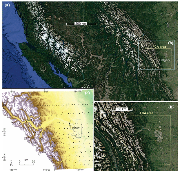
Figure 1Foothills Climate Array (FCA) study region. (a) Location within southwestern Canada, with the blue inset indicating (b) the study setting within the regional context of the Canadian Rocky Mountains and the yellow inset indicating (c) the FCA site network. Panels (a) and (b) are courtesy of Google Earth. Crosses are mountain sites and dots are prairie sites.
The data set contains the mean daily values of RH, qv, and ev over the 5-year study. The data set consists of 1826 days from 232 sites, giving a total of 423 362 records. Missing data are gap filled and flagged as “estimated”; this makes up 11 % of the data set. Section 2 describes the study area and instrument array in more detail. Sensor accuracy and quality control procedures are discussed in Sect. 3. Section 4 defines the humidity measures and discusses the calculation of daily mean values. Section 5 describes the gap-filling measures applied to the data set, and Sect. 6 summarizes the mean monthly data, its spatial patterns, and lapse rates of humidity in the study region. We summarize the data set in Sect. 8.
The Foothills Climate Array (FCA) was established in 2004 and 2005 in the foothills of the Rocky Mountains in southwestern Canada, at approximately 51∘ N and 114.5∘ W (Fig. 1). An area of roughly 18 000 km2 (120 km × 150 km) was instrumented with a two-dimensional network of automatic weather stations recording temperature, RH, and rainfall (Wood et al., 2018a). The FCA was set up in a series of east–west transects, spaced roughly 10 km apart and running from the continental divide on the western end of the study region to the flat, prairie grasslands on the eastern edge. Station spacing along the east–west transects was about 5 km in the mountains and 10 km for the sites, with lower relief on the eastern half of the study region.
The continental divide runs northwest–southeast along the western margin of the FCA. Elevations of the high peaks in the Canadian Rocky Mountains reach 3500 m, with the treeline at 2200–2600 m, depending on the aspect. The environment above the treeline consists of rock, talus, alpine lakes, and glacier cover, with sparse vegetation. Coniferous forest and alpine meadows are found below the treeline, transitioning to mixed forest (e.g., aspen) in the lower-elevation rolling hills of the Alberta foothills. This grades into shrub, grassland, and cultivated cropland in the prairies, where land use changes to ranching, farming, and urban areas. FCA sites are classified as mountain or prairie based on their elevation and terrain variability surrounding the site. Prairie sites are generally situated below 1250 m, with little terrain variability. Within this zone, nine sites are situated within the Calgary municipal boundary. Elevations drop to below 900 m at the eastern edge of the array. The study area and site locations therefore comprise a wide range of elevation, topography, and surface types.
Each FCA installation consisted of data-logging rainfall, temperature, and RH gauges mounted on a pole that was either pounded into the ground or supported with a cairn. Instantaneous T and RH were recorded every hour at the top of the hour, using SP-2000 data loggers manufactured by Veriteq Instruments Inc. (Veriteq has subsequently been bought out by Vaisala, which continues to make an adapted version of this data logger). The data loggers were mounted inside radiation shields manufactured by Onset Scientific Ltd. to protect the loggers from direct sunlight and allow air circulation. The manufacturer-reported measurement range for the RH sensors is 0 % to 95 %, with a 5-year accuracy of ±5 % between RH values of 10 % and 90 % at 25 ∘C.
Up to 244 stations were in operation during the main recording period from July 2005 to June 2010, with 232 sites having reliable data (see Sect. 3.2). Sites were visited once or twice per year for data download, instrument cleaning, and data logger replacement if required. Where possible, T and RH were recorded at a height of 1.5 m above the ground. At sites with significant snow accumulation (generally at elevations above 2000 m), pole extensions were used to keep the sensors above the winter snowpack and instrument heights were between 2 and 3 m, year-round. Sites do not conform to World Meteorological Organization (WMO) standards, which specify that climate recording sites should be level, away from vegetation and buildings, and not in areas of variable topography (WMO, 2008). This prescription is not consistent with the purpose of the study, which is to examine topographic and surface environmental influences on weather. By design, the array samples different slopes, aspects, and degrees of forest closure to quantify realistic, landscape-scale spatial variability. Examples of site locations and more details on the FCA design are provided in Wood et al. (2018a).
3.1 Sensor accuracy
Sensor calibration and quality control for the temperature data are described in detail in Wood et al. (2018a). Instruments were calibrated at the University of Calgary weather research station (WRS) before being set up in the field and on an ongoing basis during the study to assess systematic bias or drift of the sensors. This reference site records data at 1 min intervals.
For calibration tests, sensors were set to record instantaneous RH at 1, 2, or 5 min intervals for 1- to 2-week periods. To represent the actual field methodology, top-of-the hour measurements were extracted for each sensor and compared with top-of-the hour measurements at the University of Calgary WRS, which uses a Campbell Scientific HMP35CF sensor mounted in a ventilated, Gill Model 41004-5 12 plate radiation shield.
Where the mean absolute RH difference between a sensor and the WRS reference sensor is greater than 20 % (in RH, averaged over the calibration test), we assume that the sensor is malfunctioning and we exclude these data. After rejecting these sensors, the average RH difference for all calibration tests carried out from 2004 to 2011 is less than 1 %. There is variability between sensors, with WRS–Veriteq differences having a standard deviation of 6 % for all tests. Individual sensors have slightly different behaviour and some have biases of several percent, up to a maximum of 10 %. No bias or drift corrections were applied to the data as calibration tests do not show systematic bias or drift, and multiple data loggers were deployed at some sites due to sensor malfunction during the study period. Based on the calibration tests, uncertainties in RH are estimated to be 6 % (±1σ) for daily mean values, slightly greater than the instrumental accuracy. This 6 % uncertainty propagates through to the estimates of vapour pressure and specific humidity. Compounded with the uncertainty of ±0.2 ∘C in mean daily temperature (Wood et al., 2008a), through the calculation of saturation vapour pressure (Eq. 1), we estimate an accuracy of ±7 % in mean daily ev and qv. This estimate assumes that the WRS humidity data are perfectly accurate; in reality, the uncertainty will be higher.
3.2 Quality control (QC)
Erroneous temperature measurements from the Veriteq sensors are generally accompanied by unreliable RH measurements. Therefore, RH data are excluded for the 9 % of records with missing or faulty temperature measurements (see Wood et al., 2018a). Examination of the data indicates that RH can also be erroneous at times with valid temperature data. Further quality control tests were therefore carried out to exclude additional bad data due to sensors malfunctioning. While the range of the sensors is quoted as 0 %–95 %, measurements in the field ranged from 0 % to 100 %. WRS RH data ranged from 9 % to 100 % during the calibration tests. When the Veriteq sensors record RH values less than 10 %, the sensors commonly show limited variability throughout the day, likely indicating sensor malfunction. The study region is characterized by a dry, continental climate, but RH values below 10 % are deemed to be physically unlikely. Hourly values less than 10 % are therefore set to 10 %. Visual quality assessment during data downloads indicated other forms of sensor malfunction, e.g., a sensor recording a constant value while neighbouring sensors show variability or a sensor indicating extreme fluctuations compared with neighbouring sensors. These data are considered unreliable and are excluded. We also exclude days with the minimum value equal to the maximum value when not equal to 100 % and where values fluctuate repeatedly between 10 % and 100 %.
The final quality assessment test compares site daily mean and minimum values with those from a group consisting of the 30 nearest-neighbour stations. Daily maxima are not used as it was common for days to have 100 % as their maximum value. Neighbourhood means exclude sites with questionable data, based on sensors that failed any of our QC tests and days with less than 20 h of measurements. In addition, the site(s) within a group having the lowest or highest daily mean and minimum values are excluded from the neighbourhood means calculation. This step is meant to filter out anomalous local effects, which may be real but can be specific to local conditions. Site-days on which either the minimum or mean value exceeds the neighbourhood values by more than 3 standard deviations are excluded from the final data set.
The quality control steps result in the exclusion of ∼2 % of the data, in addition to the 9 % of the data that are rejected due to missing or faulty temperature readings. The final data set is 89 % complete, but missing data affect more than 90 % of the sites. We therefore estimate missing data (see Sect. 5) to allow more straightforward and reliable applications of this data set.
4.1 Calculation of vapour pressure and specific humidity
Following WMO (2008), saturation vapour pressure over water is calculated from
where T is the temperature in ∘C and the units of vapour pressure are hPa (mbar). Vapour pressure is then calculated from . Given the air pressure, P, vapour pressure can be converted to the mixing ratio, w, or specific humidity, qv. The assumption qv≈w is commonly adopted in atmospheric science (Tsonis, 2002, p. 94) and is accurate within 1 % for the range of vapour pressures in our study region (i.e., within the accuracy of our data). Specific humidity (g kg−1) is thus taken to be equivalent to the mixing ratio, calculated from
For a site with elevation z (m) and absolute temperature TK, we estimate hourly air pressure based on the assumption of a standard atmosphere, using Environment Canada data from Calgary International Airport, which has a reference elevation of z0=1099 m. For reference temperature T0 (K) and pressure P0 (hPa), pressure at each site is calculated from the hypsometric equation (e.g., Wallace and Hobbs, 1977):
Equation (3) accounts for the typical decrease in pressure with elevation. Using Eqs. (1)–(3), hourly ev and qv can be calculated from the in situ values of T and RH, along with the elevation-corrected air pressure. Uncertainties in pressure estimates from Eq. (3) are small relative to uncertainties in qv; for elevations of 2000 m, with an air pressure of ∼800 hPa, an error in P of 10 hPa results in an error in qv of 0.1 % for ev in the range 1–10 hPa.
4.2 Calculation of daily means
Due to the fact that RH is a constructed variable that depends non-linearly on both temperature and vapour pressure, calculation of mean daily humidity values is more complicated. Two different approaches are used here to calculate humidity values for the site-days having complete and valid data. The first method computes mean daily ev and qv from mean daily T and RH values. The second method calculates hourly ev and qv from the raw hourly T and RH data, then computes mean daily values of ev and qv from the arithmetic average of hourly data. Vapour pressure and specific humidity values that are computed from mean daily T and RH values are not identical to the mean of hourly ev and qv data over the day due to non-linearities in the saturation vapour pressure and the fact that RH saturates at 100 %. Method one gives mean daily values for ev and qv that are thermodynamically consistent with the mean daily temperature and RH data (Wood et al., 2018a), while method two gives a truer estimate of vapour pressure and specific humidity.
Differences between these two methods, , are plotted in Fig. 2 for all site-days as a function of mean daily temperature and daily temperature range. Differences are greatest for higher temperatures and when the diurnal temperature range is large. On days with mean temperature greater than 15 ∘C, the average Δqv is equal to 0.3 g kg−1. Saturation vapour pressure increases exponentially with temperature, so the maximum possible specific humidity during the cool hours of a day (typically overnight) is commonly an order of magnitude lower than that during the warmest hours of the day. On days with a large diurnal temperature range, low overnight values of qvh tend to decrease the average daily specific humidity. Hence, Δqvis generally positive for temperatures greater than 0 ∘C and increasingly so on warm days with a high diurnal range. This is also true for the percentage difference (Fig. 2c and d), where Δqv has a roughly linear relationship with both temperature and diurnal temperature amplitude across the full range of observed conditions (with exceptions to this behaviour). Relative differences vary from −10 % to +10 %. For mean daily temperatures of −10 to +10 ∘C, the effect is less than 3 %. Absolute differences are generally less than 0.1 g kg−1 on cold days ( ∘C), as specific humidity is low.
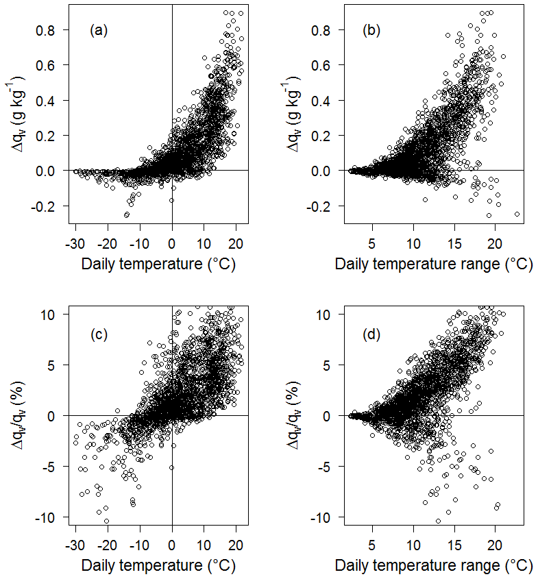
Figure 2Relation between Δqv and (a, c) daily mean temperature and (b, d) daily temperature range. Δqv is the difference in specific humidity calculated from daily mean T and RH (qvd) and from the mean of hourly qv data (qvh): . The top panels are actual differences, in g kg−1, and the lower panels are normalized by qvd, expressed as the percent difference.
The hourly data give truer values of daily mean vapour pressure and specific humidity: this is the most accurate estimate of how much water vapour is present on a given day. These values are recommended for applications that require daily mean values, such as calculations of precipitable water, parameterizations of incoming longwave radiation (Brutsaert, 1975; Sedlar and Hock, 2009), or latent heat flux calculations in boundary layer meteorology (e.g., Oke, 1987; Andreas, 2002). We recognize that these values of ev and qv are not thermodynamically consistent with the daily mean values of T and RH in our data set. Hence, we also provide daily mean estimates of ev and qv that are based on the daily average temperature and RH. These are recommended for some applications, e.g., those which use vapour pressure deficit, which require estimates of es from mean daily temperature.
Spatial interpolation methods such as inverse-distance weighting (IDW) or kriging can be used to interpolate spatially autocorrelated data (e.g., Ozelkan et al., 2015). For large areas with small variations in topography, a combination of multiple regression using horizontal location and elevation- and inverse-distance-squared weighted interpolation (gradient-plus-inverse distance squared or GIDS) has been used by Nalder and Wein (1998); however, there is variable topography in the FCA area and humidity does not always vary systematically with elevation, so this method is not suitable. Co-kriging, as used by Ishida and Kawashima (1993), explicitly controls for elevation by including elevation as a covariate. Apaydin et al. (2004) apply co-kriging with elevation for interpolating different meteorological variables in southeastern Turkey. They recommend co-kriging for spatial interpolation of most variables, including RH.
Using Eqs. (1)–(3), qv can be calculated from T, RH, and P. Mean daily temperature data used for the humidity calculations are complete, based on gap-filling strategies detailed in Wood et al. (2018a). Hourly temperature data are not available for the 11 % of site-days with missing data; therefore, humidity variables are calculated using mean daily values for the missing data. Spatial interpolation can be applied to either qvd or RH to estimate missing values. The resulting values are then used to calculate the other unknown (either qvd or RH); this is again required for thermodynamic consistency, as independent interpolations of both qvd and RH at a site give values that are inconsistent with the daily mean temperature.
In this study we tested IDW and kriging methods on both daily mean qv and RH. Both data sets exhibit positive spatial autocorrelation, with RH showing no correlation with elevation and qv moderately correlated with elevation. Leave-one-out cross validation was used to determine the best method and parameters for estimating missing data. With this method, the model is run as many times as there are data points, excluding a different data point for each run, and the remainder of the data are used to estimate the removed point. Using cross-validation, various error measures can be calculated by comparing predicted and observed values, e.g., root mean square errors (RMSEs) and mean absolute errors (MAEs).
The IDW technique considers a number of points within a neighbourhood of the target location, with contributions weighted inversely according to the distance between each point and the site of interest. The rate of decay can be varied by applying a power function to the separation distance. Higher powers increase the weighting of nearby points relative to more distant points. IDW interpolation models were run for each day, leaving each site out in turn and using the remaining sites to predict the omitted site. Models were run with the power parameter varying from 1 to 3.5 in 0.25 increments and using between 5 and 30 neighbours. Errors are calculated as the difference between the estimated and measured values. The MAE and RMSE are calculated for the 2006 data for each combination of power and number of neighbours. Interpolating qv and then calculating RH generates some unrealistic RH values, greater than 100 %. In this event, RH was set to 100 % and qv was recalculated. This gives physically consistent values of qv, temperature, pressure, and RH.
Kriging also considers a number of points within a neighbourhood, but the relative contributions are based on a semi-variogram, which models the distance–variance function calculated from all points within a predefined range. The co-kriging model included elevation as a covariate with qv, where neighbourhood weights are based on a cross-semi-variogram modelled on the covariance between elevation and qv. The spatial relationship can be modelled using different functions, e.g., spherical or exponential, and varying the values for the sill, nugget, and range parameters (e.g., Isaaks and Srivastava, 1989). The range represents the limit of correlation between sites, the sill represents the maximum variance between sites, and the nugget represents the minimum variance between close sites. The semi-variogram function groups sites into bins based on separation distance, and the variance between sites can differ on a daily basis. Semi-variogram models were produced for annual aggregated data (annual mean value for each site), monthly aggregated data (mean monthly value for each site), and for daily data. These models are used to estimate each site-day using leave-one-out cross-validation.
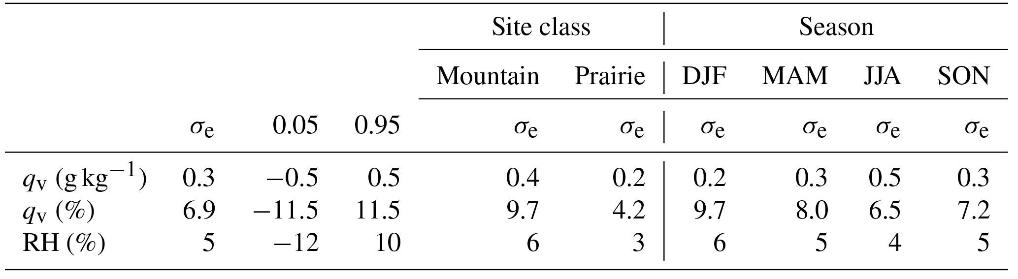
Table 1Spatial interpolation errors for qv and RH by site class (mountain vs. prairie site) and season. σe is the standard error (the standard deviation of the error distribution) and 0.05 and 0.95 are the 5th and 95th percentile values of the error.
Differences in MAE are small for the different interpolation methods (IDW and kriging), variables (qv and RH), and model parameters. The model with the lowest MAE for both qv and RH uses IDW interpolation with a power of 2. It is difficult to select which humidity variable is better to interpolate based on MAE only, although qv is intuitively favourable since it is a continuous variable and an actual physical field, rather than a construct of two different variables (temperature and vapour pressure), with a saturation point (100 %). As an additional test, Fig. 3 plots the frequency distribution of actual and interpolated qv and RH values. These plots are generated from the cross-validation data for the full data set, comparing interpolated and actual values for all known points. The two-sample Kolmogorov–Smirnov test determines whether two samples have similar cumulative probability distribution functions. Estimated and actual qv distributions are statistically similar at the 95 % significance level, but RH distributions differ, as is visible in the stronger mode at 100 % in the interpolated values (Fig. 3d). We cannot infer whether this is due to the saturation at 100 % or the non-linearities in the saturation vapour pressure (i.e., in hourly vs. daily estimates). These differences support the case for interpolating qv rather than RH. We therefore fill data gaps based on an IDW interpolation of daily mean T and qvd. Daily mean ev and RH are then calculated from the interpolated local values of T and qvd. The optimal IDW interpolation uses a power of 2 with 18 neighbours.
Table 2(a) Monthly means (and standard deviations) of temperature, relative humidity, vapour pressure, and specific humidity across all FCA sites. Standard deviation refers to the spatial variability in mean monthly values. (b) Mean monthly lapse rates of relative and specific humidity, based on a linear regression with elevation: and . R2 values from the linear regressions are given in brackets. Italicized values are statistically significant (p<0.01).
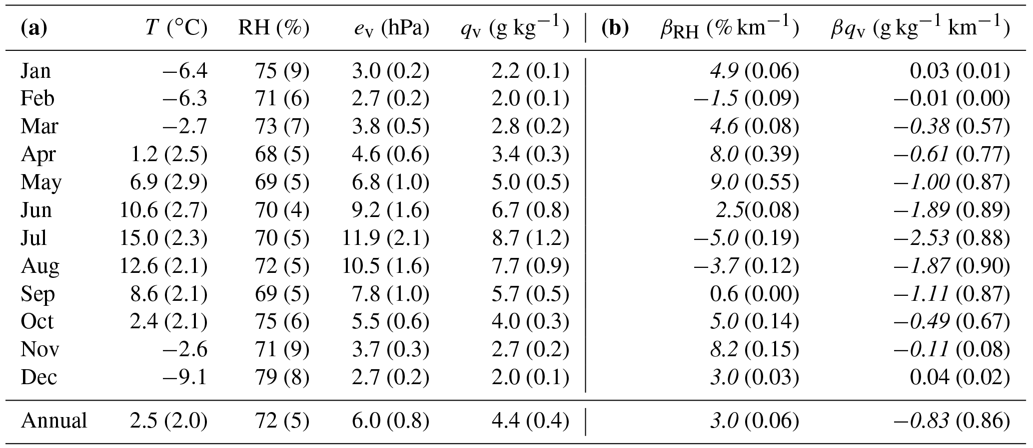
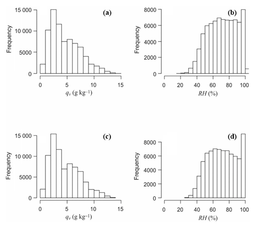
Figure 3Frequency distributions of (a, b) actual and (c, d) interpolated specific and relative humidity. Interpolated values are calculated from the optimized IDW model applied to all sites in the cross-validation (leave-one-out) experiments.
Table 1 summarizes the distribution of the validation interpolation errors for mountain and prairie sites and for all sites as a function of season. Average interpolation errors for qvd are 0.3 g kg−1, and 90 % of estimated qvd values are within ±0.5 g kg−1 of the actual values. Errors are greater for the mountain sites than in the prairies, and absolute errors increase with warmer temperatures, from 0.2 g kg−1 in winter to 0.5 g kg−1 in summer. As a percentage relative to the mean seasonal values, errors in qvd have the opposite relationship, at 10 % in the winter months and 6 % in the summer. For interpolations of RH, mean absolute errors average 5 %, with 90 % of values in the range −12 % to +10 %. Similarly to qvd, average errors at mountain sites are twice as large as in the prairies (6 % vs. 3 %) and are slightly higher in the winter season.
Table 2 summarizes the monthly mean values of temperature and each humidity variable over the study area, based on the hourly data. Spatial variability across the FCA is represented through the standard deviation in each value (N=232). Monthly mean values neglect the spatial richness of the data set, but they illustrate the mean climatology and seasonal cycle of humidity variables in this region. For reference, the average elevation of FCA sites is 1480 m. Figure 4 plots mean annual ev, qv, and RH vs. T at each FCA site, based on the 5-year averages. Each variable has a significant relation with temperature, with ev and qv decreasing with decreasing temperature and RH increasing. This accounts for much of the observed elevation dependence.
As seen in Table 2, RH has a moderate seasonal cycle, averaging 70 % in summer (JJA) and 75 % in winter (DJF), with greater spatial variability in the study region in the winter months (±5 % and ±8 % for the two seasons, respectively). Vapour pressure and specific humidity are strongly correlated, so we primarily discuss the latter. These two variables have a strong seasonal cycle associated with temperature controls on atmospheric moisture and increased warm-season evapotranspiration. Mean winter and summer values for qv are 2.1 and 7.7 g kg−1, with a maximum in July. Spatial variability is much greater in the warm season, with the standard deviation of mean monthly values across the FCA equal to 0.1 g kg−1 (5 %) in the winter and to 0.9 g kg−1 (12 %) in the summer (Table 2).
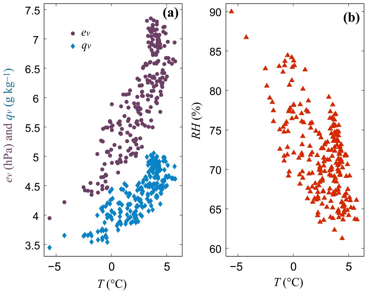
Figure 4Mean annual humidity data as a function of mean annual temperature at each FCA site. (a) Vapour pressure (brown circles) and specific humidity (blue diamonds). (b) Relative humidity (red triangles).
The gap-filled data set is used to visually examine spatial and seasonal patterns of qv and RH in the FCA. Figure 5 plots the spatial distribution of mean seasonal qv across the study region. This illustrates the relatively low spatial variance in winter. Locations in the foothills that are slightly drier in the winter season may be capturing the regional chinook belt (Nkemdirim, 1996; Cullen and Marshall, 2011), which runs northwest to southeast in the lee of the Rocky Mountains. The other three seasons are characterized by strong longitudinal and altitudinal gradients in specific humidity, with more humid conditions on the lower-elevation, agricultural lands in the eastern section of the FCA. The city of Calgary has no apparent influence on humidity patterns. There is a lot of spatial structure in the mountains in all seasons. In the autumn and winter, there is evidence of humid Pacific air masses that cross over the continental divide into the western part of the study area, particularly in the central region. The Bow River is also evident in these plots at the mountain sites, running eastwards between Banff and Calgary (see Fig. 1). More humid conditions are recorded at sites adjacent to the river, typically ∼1 g kg−1 greater than at neighbouring sites to the north and south. This indicates that the river provides a significant local source of near-surface moisture in the mountains. This influence is not discernible at the more humid prairie sites.
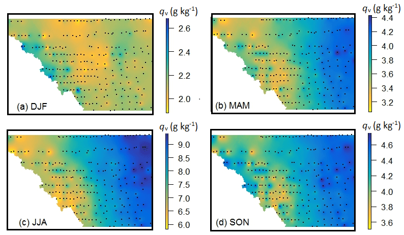
Figure 5Mean seasonal values of specific humidity over the study region (g kg−1): (a) winter (DJF), (b) spring (MAM), (c) summer (JJA), and (d) autumn (SON).
Figure 6 plots the seasonal relation between specific humidity, elevation, and longitude in the study region. Vertical gradients (lapse rates) of qv and RH are given in Table 2, calculated from a linear regression of mean monthly values vs. elevation. There is a strong elevational dependence from March to October, with significant regressions (p<0.01) and R2 values greater than 0.8 in all cases. The mean qv lapse rate in summer is −2.1 g kg−1 km−1, a strong decrease in qv with elevation. Relative to the mean summer value of 7.7 g kg−1 in the study area, this is a decline of 27 % per 1000 m of elevation. Specific humidity lapse rates in autumn and spring are also significant, but weaker (roughly −17 % per 1000 m). Autumn has more scatter (Fig. 6a), possibly because September has transitional summer to autumn weather patterns in the study region. Consistent with Fig. 5, there is no relationship between qv and elevation in the winter months.

Figure 6Mean seasonal specific humidity vs. (a) elevation and (b) longitude, for all sites. Values are a composite of 5 years in each seasonal record (i.e., average specific humidity at each site over 15 months). Winter (DJF) is shown in blue asterisks, spring (MAM) in green diamonds, summer (JJA) in red stars, and autumn (SON) in orange circles.
Relative humidity has a weaker relationship with elevation than qv, with a variable sign and lower R2 values (Table 2). Elevation explains only a small proportion of the variance in RH, from 0 % to 55 %, but most months still have statistically significant regression coefficients against elevation. Hence, elevation-based models would have weak predictive skill for modelling the spatial variation of RH in the study region, but there are underlying elevation trends. In most months RH increases with elevation, indicating conditions closer to saturation at high elevations in the study area. This is the particularly notable in April and May (average RH increase of 8.5 % km−1), when the RH regressions against elevation are strongest. Elevation regressions have the opposite sign in July and August, with an average RH lapse rate of −4.4 % km−1. Specific humidity also decreases strongly with elevation in these peak summer months. Summer evapotranspirative moisture sources in the grass- and croplands in eastern portions of the study area (Taylor et al., 2011) may contribute to higher low-elevation qv levels (Fig. 6b). It is difficult to separate the effects of elevation from longitude in the data, as these are strongly correlated (). Humidity patterns also reflect the regional temperature structure associated with thermodynamic limits on the amount of water vapour and the direct influence of temperature on RH (Fig. 4).
Daily humidity structure can be much more complex than the seasonal and annual mean patterns. Different air masses impact the study region, associated with synoptic- and regional-scale weather patterns that cover all or part of the FCA on a given day. Examples include extratropical cyclones that can stall at the mountain barrier, advecting mild, humid air from the southeast (e.g., Milrad et al., 2015); hot summer days that give rise to local- to regional-scale convective instability and dry line development (Taylor et al., 2011); continental polar air masses from the north (Cullen and Marshall, 2011); and chinook conditions that can occur under strong westerlies (Nkemdirim, 1996). Each of these weather types can be expected to have characteristic humidity patterns.
As examples, Fig. 7 shows daily mean qv and RH structure across the FCA for each of the weather systems outlined above. The cyclonic system in Fig. 7a and b gives a good representation of elevation and temperature controls on specific humidity, as RH is ∼100 % over the entire domain. Cloud cover and precipitation extend over the region and there is a strong source of moisture advection, so there are primarily thermodynamic constraints on specific humidity (saturation). The example in Fig. 7c and d is for a hot summer day with localized thunderstorm activity. There is a strong contrast between mountain and prairie sites, and qv and RH are highly correlated. Evapotranspiration in the prairie croplands may be providing a source of near-surface moisture on the eastern portion of the domain. Relative to the surrounding agricultural areas, the city of Calgary has lower qv and RH levels.
The bottom four panels in Fig. 7 are for winter weather systems. These illustrate the contrasting influences of a cold, continental air mass that pushes into the region from the northeast (Fig. 7e and f) and chinook winds from the west (Fig. 7g and h). For both examples, qv and RH increase with elevation in the western portion of the study region. The humidity–elevation relationships are opposite in sign to the summer systems (Fig. 7a to d). The continental polar air mass that sits over the prairies in Fig. 7e and f is cold ( ∘C), dry (qv<2 g kg−1), and near saturation, with RH ≈90 %. Conditions are exceptionally uniform over the prairies. The western section of the study area was under the influence of a westerly (Pacific) air mass on this day. This brought mixed rain and snow to the mountain sites on this day, with qv∼5 g kg−1 and an average temperature of 0.7 ∘C in Banff, Alberta. A clear transition zone in the foothills separates the Pacific and Arctic air masses, with intermediate values of qv, milder temperatures than the prairies, and lower RH.
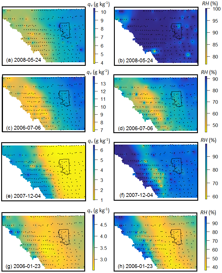
Figure 7Examples of daily specific (a, c, e, g) and relative (b, d, f, h) humidity structure in the study area. (a, b) A cyclonic precipitation event on 24 May 2008. (c, d) A day with afternoon thunderstorm activity on 6 July 2006. (e, f) A continental polar air mass over the study area on 4 December 2007. (g, h) Chinook conditions on 23 January 2006.
The chinook day in Fig. 7g and h features high humidity levels along the continental divide and low values (qv<2 g kg−1 and RH <50 %) across the foothills and prairies. Chinook winds are associated with dry-adiabatic descent in the lee of the Rockies, bringing warm and dry conditions. Figure 7g and h are classic examples of this, with the chinook belt evident over an ∼80 km wide swath that parallels the continental divide. High-elevation sites near the continental divide are experiencing cloud cover, strong winds, and intermittent precipitation. Chinook effects weaken east and north of Calgary, with higher qv and RH. Conditions like these two winter examples are frequent in the cold season, with moist Pacific air masses penetrating over the continental divide and reaching high-elevation sites on the western portion of the grid. The contrast with cold, dry continental air over the prairies creates a humidity inversion with altitude.
The examples in Fig. 7 demonstrate the richness of the data set and its potential value for different meteorological, ecological, hydrological, and agricultural applications. While there is systematic structure in the seasonal and annual humidity patterns, daily humidity patterns can deviate strongly from this. Additional studies are needed to analyse the interaction of weather systems with terrain and surface cover in the study region, but humidity patterns can help to understand this interaction. These examples also reveal the importance of considering daily weather systems as well as seasonal cycles in algorithms, which downscale humidity distributions over the terrain, e.g., from climate model reanalyses or projections (e.g., Abatzoglou, 2013; Pierce and Cayan, 2016).
Data described are available on the PANGAEA repository, https://doi.org/10.1594/PANGAEA.889435 (Wood et al., 2018b), with links to the associated temperature data (Wood et al., 2017). Mean daily temperature, pressure, vapour pressure, relative humidity, and specific humidity data are available at each of the 232 sites for the period 1 July 2005 to 30 June 2010. Site latitude, longitude, elevation, land surface type, and sensor height above ground are also noted, and there is a flag to mark whether humidity data for each site-day are directly measured or estimated (interpolated). Where measured data are available, we provide daily mean vapour pressure and specific humidity estimates calculated using both hourly and daily measurements (see Sect. 4.2).
The Foothills Climate Array (FCA) offers a unique collection of high-density, multi-year observations in complex mountain terrain. These data provide a detailed view of near-surface humidity patterns, lapse rates, and their temporal variability, with potential applications in hydrological, ecological, or agricultural models that require surface energy balance calculations or humidity estimates in complex terrain. The data also provide a detailed view of regional weather system interactions and their interaction in mountain terrain, e.g., dry line and front propagation; chinook structure. This paper presents the data set, quality control, and gap-filling strategies used to process the data, and basic characteristics of the data set, including monthly means of specific and relative humidity and their relation with temperature, elevation, and longitude in the study area.
The Veriteq relative humidity instruments used in this study performed well, with some variability between sensors. Quality control procedures were successful in identifying and removing questionable data, resulting in 11 % of missing data. We gap filled the data that are available here using spatial interpolation, with a flag to denote data that have been estimated. Validation of our gap-filling method for sites with known data indicates average errors of ±7 % in the interpolated qv and RH data. Errors are higher in the winter (±10 %).
Errors also result from the method chosen to calculate daily means, but in this case the errors can be systematic (i.e., a consistent bias). Specifically, specific humidity calculated using mean daily T and RH can deviate by up to ±10 % from the “true” daily means that are calculated using hourly data. This effect is greatest for high temperatures and when there is a large diurnal temperature range. We present daily mean ev and qv using both methods: (i) hourly means of ev and qv and (ii) daily means calculated from mean daily T and RH. The former are recommended as they provide a better estimate of actual atmospheric water vapour over the day, but we note that the resulting values of mean daily ev and qv are not thermodynamically consistent with the mean daily T and RH. In addition, values from method (i) are not available for the gap-filled records.
Monthly mean specific and relative humidity have significant relations with temperature, elevation, and longitude in our study area. Sites on the eastern portion of our grid have higher qv in all seasons but winter, with the strongest contrasts in the summer. The average annual qv gradient with elevation is −0.83 g kg−1 km−1, reflecting the cooler, drier air at higher altitudes. Summer lapse rates average −2.1 g kg−1 km−1, spring and autumn values average −0.7 g kg−1 km−1, and there is no relation between qv and elevation from November to February due to frequent humidity inversions in the study region. Relative humidity has statistically significant relations with elevation in most months, with a general trend of increasing RH with elevation and an average annual gradient of +3 % km−1. However, elevation explains only a small amount of the variance in RH and this relation changes sign in the summer, with RH decreasing with elevation in July and August.
Depending on the weather system and air mass that are in the region, spatial humidity patterns in the daily data can diverge markedly from the average seasonal and annual patterns. This is a significant challenge for downscaling or interpolating humidity fields in complex terrain. For applications requiring daily data, it may be fruitful to consider humidity structure as a function of the prevailing weather system. As an intermediate step to resolve some of the systematic spatial and temporal humidity structure, downscaling of humidity fields could be done using monthly or seasonal elevation gradients (lapse rates). For interpolation and downscaling of humidity fields, we recommend working with specific humidity and temperature, then calculating RH from the results, as these are more primary physical variables.
The authors declare that they have no conflict of interest.
This article is part of the special issue “Water, ecosystem, cryosphere, and climate data from the interior of western Canada and other cold regions”. It is not associated with a conference.
The Foothills Climate Array was funded by the Canada Foundation for
Innovation, the Natural Sciences and Engineering Research Council (NSERC) of
Canada, and the Canada Research Chairs programme. We thank Rick Smith at the
University of Calgary weather research station for his invaluable help over
the lifetime of the FCA study. Graduate and undergraduate students, summer
research assistants, friends, and volunteers that contributed to the FCA
study are too numerous to list, but prominent within this group are Terri Whitehead, Kara Przeczek, and Bridget Linder. We could not have managed this
study without their dedication and enthusiasm. We thank the managing editor,
Warren Helgason, along with Paul Whitfield and an anonymous reviewer for
their comments and suggestions, which have improved this manuscript.
Edited by: Warren D. Helgason
Reviewed by: Paul Whitfield and one anonymous referee
Abatzoglou, J. T.: Development of gridded surface meteorological data for ecological applications and modelling, Int. J. Climatol., 33, 121–131, https://doi.org/10.1002/joc.3413, 2013.
Andreas, E. L.: Parameterizing scalar transfer over snow and ice: a review, J. Hydrometeorol., 3, 417–432, 2002.
Apaydin, H., Sonmez, F. K., and Yildirim, Y. E.: Spatial interpolation techniques for climate data in the GAP region in Turkey, Clim. Res., 28, 31–40, 2004.
Brutsaert, W.: On a derivable formula for long-wave radiation from clear skies, Water Resour. Res., 11, 742–744, 1975.
Buzan, J. R., Oleson, K., and Huber, M.: Implementation and comparison of a suite of heat stress metrics within the Community Land Model version 4.5, Geosci. Model Dev., 8, 151–170, https://doi.org/10.5194/gmd-8-151-2015, 2015.
Cullen, R. M. and Marshall, S. J.: Mesoscale temperature patterns in the Rocky Mountains and foothills region of southern Alberta, Atmos. Ocean, 49, 189–205, https://doi.org/10.1080/07055900.2011.592130, 2011.
Eamus, D., Boulain, N., Cleverly, J., and Breshears, D. D.: Global change-type drought-induced tree mortality: vapor pressure deficit is more important than temperature per se in causing decline in tree health, Ecol. Evol., 3, 2711–2729, https://doi.org/10.1002/ece3.664, 2013.
Epstein, Y. and Moran, D. S.: Thermal comfort and the heat stress indices, Indust. Health, 44, 388–398, 2006.
Hoch, J. and Markowski, P.: A climatology of springtime dryline position in the U.S. Great Plains region, J. Climate, 18, 2132–2137, 2005.
Holden, Z. A. and Joly, W. M.: Modeling topographic influences on fuel moisture and fire danger in complex terrain to improve wildland fire management decision support, Forest Ecol. Manag., 262, 2133–2141, https://doi.org/10.1016/j.foreco.2011.08.002, 2011.
Isaaks, E. H. and Srivastava, R. M.: An Introduction to Applied Geostatistics, Oxford University Press, New York, USA, 1989.
Ishida, T. and Kawashima, S.: Use of Cokriging to Estimate Surface Air-Temperature from Elevation, Theor. Appl. Climatol., 47, 147–157, 1993.
Johnson, Z. F. and Hitchens, N. M.: Effects of soil moisture on the longitudinal dryline position in the southern Great Plains, J. Hydrometeor., 19, 273–287, https://doi.org/10.1175/JHM-D-17-0091.1, 2018.
Lengfeld, K. and Ament, F.: Observing local-scale variability of near-surface temperature and humidity using a wireless sensor network, J. Appl. Meteorol. Clim., 51, 30–41, https://doi.org/10.1175/JAMC-D-11-025.1, 2012.
Marks, D. and Dozier, J.: Climate and energy exchange at the snow surface in the alpine region of the Sierra Nevada. 2. Snow cover energy balance, Water Resour. Res., 28, 3043–3054, 1992.
Masterson, J. M. and Richardson, F. A.: Humidex, a method of quantifying human discomfort due to excessive heat and humidity, Environment Canada, Atmospheric Environment Service, Downsview, Ontario, Canada, CLI 1-79, 1979.
Milrad, S. M., Gyakum, J. R,. and Atallah, E. H.: A meteorological analysis of the 2013 Alberta flood: Antecedent large-scale flow pattern and synoptic–dynamic characteristics, Mon. Weather Rev., 143, 2817–2841, https://doi.org/10.1175/MWR-D-14-00236.1, 2015.
Nalder, I. and Wein, R.: Spatial interpolation of climatic Normals: test of a new method in the Canadian boreal forest, Agr. Forest Meteorol., 92, 211–225, 1998.
Nkemdirim, L.: Canada's chinook belt, Int. J. Climatol., 16, 441–462, 1996.
Oke, T. R.: Boundary Layer Climates, 2nd Ed, Psychology Press, New York, USA, 435 pp., 1987.
Ozelkan, E., Bagis, S., Ozelkan, E. C., Ustundag, B. B., Yucel, M., and Ormeci, C.: Spatial interpolation of climatic variables using land surface temperature and modified inverse distance weighting, Int. J. Remote Sens., 36, 1000–1025, 2015.
Pechony, O. and Shindell, D. T.: Fire parameterization on a global scale, J. Geophys. Res.-Atmos., 114, D16115, https://doi.org/10.1029/2009JD011927, 2009.
Pierce, D. W. and Cayan, D. R.: Downscaling humidity with Localized Constructed Analogs (LOCA) over the conterminous United States, Clim. Dynam., 47, 411–431, https://doi.org/10.1007/s00382-015-2845-1, 2016.
Polonio, D. and Soler, M.: Surface fluxes estimation over agricultural areas. Comparison of methods and the effects of land surface inhomogeneity, Theor. Appl. Climatol., 67, 65–79, https://doi.org/10.1007/s007040070016, 2000.
Rangwala, I.: Amplified water vapour feedback at high altitudes during winter, Int. J. Climatol., 33, 897–903, https://doi.org/10.1002/joc.3477, 2013.
Ruckstuhl, C., Philipona, R., Morland, J., and Ohmura, A.: Observed relationship between surface specific humidity, integrated water vapor, and longwave downward radiation at different altitudes, J. Geophys. Res., 112, D03302, https://doi.org/10.1029/2006JD007850, 2007.
Sanginés de Cárcer, P., Vitasse, Y., Peñuelas, J., Jassey, V. E. J., Buttler, A., and Signarbieux, C.: Vapor-pressure deficit and extreme climatic variables limit tree growth, Glob. Change Biol., 24, 1108–1122, https://doi.org/10.1111/gcb.13973, 2017.
Seager, R., Hooks, A., Williams, A. P., Cook, B., Nakamura, J., and Henderson, N.: Climatology, variability, and trends in the U.S. vapor pressure deficit, an important fire-related meteorological quantity, J. Appl. Meteorol. Clim., 54, 1121–1141, https://doi.org/10.1175/JAMC-D-14-0321.1, 2015.
Sedano, F. and Randerson, J. T.: Multi-scale influence of vapor pressure deficit on fire ignition and spread in boreal forest ecosystems, Biogeosciences, 11, 3739–3755, https://doi.org/10.5194/bg-11-3739-2014, 2014.
Sedlar, J. and Hock, R.: Testing longwave radiation parameterizations under clear and overcast skies at Storglaciären, Sweden, The Cryosphere, 3, 75–84, https://doi.org/10.5194/tc-3-75-2009, 2009.
Segal, M., Kallos, G., Brown, J., and Mandel, M.: Morning temporal variations of shelter-level specific humidity, J. Appl. Meteorol., 31, 74–85, 1992.
Silvestrini, R. A., Soares, B. S., Nepstad, D., Coe, M., Rodrigues, H., and Assuncao, R.: Simulating fire regimes in the Amazon in response to climate change and deforestation, Ecol. Appl., 21, 1573–1590, 2011.
Steadman, R. G.: A universal scale of apparent temperature, J. Climatol. Appl. Meteorol., 23, 1674–1687, 1984.
Taylor, N. M., Sills, D. M., Hanesiak, J. M., Milbrandt, J. A., Smith, C. D., Strong, G. S., Skone, S. H., McCarthy, P. J., and Brimelow, J. C.: The Understanding Severe Thunderstorms and Alberta Boundary Layers Experiment (UNSTABLE) 2008, B. Am. Meteorol. Soc., 92, 739–763, https://doi.org/10.1175/2011BAMS2994.1, 2011.
Tsonis, A. A.: An Introduction to Atmospheric Thermodynamics, Cambridge University Press, Cambridge, UK, 2002.
Wallace, J. M. and Hobbs, P. V.: Atmospheric Science: An Introductory Survey, Academic Press, London, UK, 55–57, 1977.
Wood, W. H., Marshall, S. J., Fargey, S. E., and Whitehead, T. L.: Daily temperature data from the Foothills Climate Array mesonet, Canadian Rocky Mountains, 2005–2010, PANGAEA, https://doi.org/10.1594/PANGAEA.880611, 2017.
Wood, W. H., Marshall, S. J., Whitehead, T. L., and Fargey, S. E.: Daily temperature records from a mesonet in the foothills of the Canadian Rocky Mountains, 2005–2010, Earth Syst. Sci. Data, 10, 595–607, https://doi.org/10.5194/essd-10-595-2018, 2018a.
Wood, W. H., Marshall, S. J., Fargey, S. E., and Whitehead, T.L.: Near-surface atmospheric humidity data from a mesoscale meteorological network in the foothills of the Canadian Rocky Mountains, 2005–2010, PANGAEA, https://doi.org/10.1594/PANGAEA.889435, 2018b.
World Meteorological Organization: Guide to meteorological instruments and methods of observations, 7th edn., World Meteorological organization, Geneva, Switzerland, 2008.
Ziegler, C. L., Lee, T. J., and Pielke Sr., R. A.: Convection initiation at the dryline: A modeling study, Mon. Weather Rev., 125, 1001–1026, 1997.
Zuliani, A., Massolo, A., Lysyk, T., Johnson, G., Marshall, S., Berger, K., and Cork, S. C.: Modelling the northward expansion of Culicoides Sonorensis (Diptera Ceratopogonidea) under future climate scenarios, PLoS ONE, 10, e0130294, https://doi.org/10.1371/journal/pone.0130294, 2015.