Comprehensive aerosol and gas data set from the Sydney Particle Study

The Sydney Particle Study involved the comprehensive measurement of meteorology, particles and gases at a location in western Sydney during February–March 2011 and April–May 2012. The aim of this study was to increase scientific understanding of particle formation and transformations in the Sydney airshed. In this paper we describe the methods used to collect and analyse particle and gaseous samples, as well as the methods employed for the continuous measurement of particle concentrations, particle microphysical properties, and gaseous concentrations. This paper also provides a description of the data collected and is a metadata record for the data sets published in Keywood et al. (2016a, https://doi.org/10.4225/08/57903B83D6A5D) and Keywood et al. (2016b, https://doi.org/10.4225/08/5791B5528BD63).

1 Introduction

Atmospheric particles adversely effect human health, impacting mortality and morbidity (Pope et al., 2002), and are a significant contributor to outdoor air pollution as well as recognized by the World Health Organization as carcinogenic to humans (Lim et al., 2012). Atmospheric particles are derived from a wide range of natural and anthropogenic sources, and hence are made up of a range of sizes and chemical compositions. This makes reduction of particle concentrations in the atmosphere by source regulation very challenging. In particular, reduction of secondary particles, which can be an important component of total particle exposure (Brook et al., 2010), is generated by photochemical reactions in the atmosphere and hence requires control mechanisms that consider the relevant gas-phase precursors to these particles.

In the most recent Australian State of the Environment Report, air quality standards were most often exceeded for fine particles in the capital cities, whilst ozone and nitrogen dioxide standards were not exceeded (Keywood et al., 2017). Currently, the highest episodes of particle pollution in Sydney can be ascribed to the presence of bushfire and dust plumes in the Sydney airshed (e.g. Johnston et al., 2011). However, significant increases in the frequency of hot days, drought, and high-fire-risk weather have been projected for New South Wales, Australia (Whetton et al., 2015). The increased frequency of hot and sunny days has been linked to photochemical smog severity (Schnell and Prather, 2017). Thus projected warmer conditions are likely to have implications for air pollution and health in New South Wales, Australia.

Comprehensive chemical transport modelling tools can be used to assist in the development of a long-term control strategy for particles in the Sydney airshed. Such models should encompass comprehensive three-dimensional simulations of the atmosphere, sources, and multi-phase chemistry that occur and should be informed by understanding of the contribution made by both local and remote particle sources to total particle exposure within the region. Ultimately such understanding should be underpinned by detailed and high-quality experimental studies.

The Sydney Particle Study (SPS) aimed to increase scientific knowledge of the processes leading to particle formation and transformations in Sydney through two comprehensive observation programmes. The groups that contributed to these observation programmes included CSIRO, NSW Office of Environment and Heritage, ANSTO, Queensland University of Technology, the Shanghai Institute of Applied Physics, and the University of Wollongong. Observations made included the collection of samples for chemical analysis (aerosol composition, acid–alkaline gases, speciated volatile organic compounds (VOCs) including alkanes, aromatics, carbonyls, isoprene and monoterpenes). In addition, continuous or semi-continuous measurements were made of aerosol number size distributions, aerosol mass, aerosol light scattering, aerosol composition, and the gaseous criteria pollutants, oxides of nitrogen, carbon monoxide, sulfur dioxide, and ozone (NO_x, CO, SO₂, O₃). Measurements were also made of meteorological parameters (wind speed, wind direction, temperature, relative humidity, radiation, boundary layer height) and atmospheric radon-222 (radon) concentration.

2 Measurement site

Measurements were made at the Westmead air quality station operated by the New South Wales Office of Environment and Heritage, located 24 km to the west of Sydney, Australia. The population of Sydney was 4.61 million in 2011 (ABS, 2011), making Sydney the largest urban centre in Australia. Sydney is a coastal city with coastline to its east and elevated forested terrain (up to 1000 m) to the north, west, and south. The climate is temperate with uniform rainfall, warm summers, and cool winters.

The SPS observations occurred in two time periods: summer 2011 (5 February–7 March 2011 SPS-I) and autumn 2012 (16 April–14 May 2012 SPS-II).

3 Instruments and methods

The sampling programme included the measurement of aerosols; criteria gases including NO_x, CO, SO₂, and ozone; acid–alkaline gases including NH₃, SO₂, HCl and HNO₃; speciated VOCs (including carbonyls); and meteorological parameters, including temperature, relative humidity (RH), wind speed–direction, and boundary layer height. Aerosols were measured with continuous or semi-continuous methods, including the measurement of aerosol mass, light scattering, and number size distributions as well as integrated measurements of aerosol composition. Atmospheric radon concentrations were also measured and provided as an indicator of transport and vertical mixing processes as described in Chambers et al. (2019).

Two integrated samples (particles, VOCs, and acid–alkaline gas) were collected each day (morning 05:00 to 10:00 and afternoon 11:00–19:00). Note that these times were local time (GMT+11 for SPS-I, GMT+10 for SPS-II). In addition, a third VOC sample was collected between 19:00 and 05:00 (i.e. overnight).

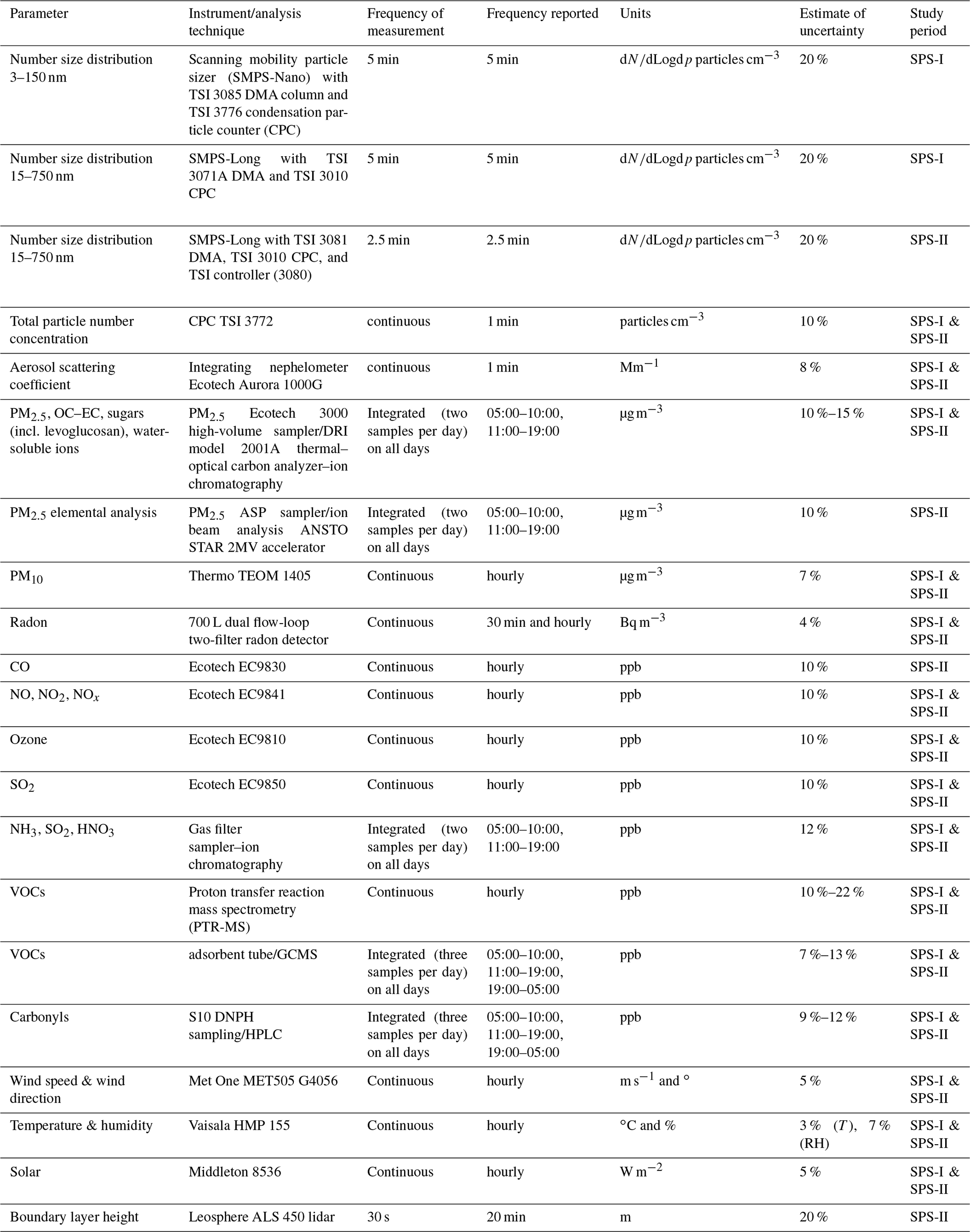
Table 1 provides a summary of the parameter measured and the instrument used to measure the parameter. The frequency at which the measurement of each parameter was made is also listed in the table, ranging from continuous to one measurement every few minutes to the collection of a sample over several hours (integrated). The frequency at which the data are reported is also included in Table 1 as well as the units that the measurements are reported in, and estimates of the uncertainty of the measurements and whether the measurements were made during SPS-I, SPS-II, or during both periods are included.

Table 1 Measurements made at Westmead during SPS-I and SPS-II along with the instrument or analytical technique employed, the measurement and reporting resolution, and the measurement units. Frequency of measurement is the frequency with which the data are collected. Frequency reported is the frequency at which the data are reported (may be an average of the frequency of measurement).

3.1 Continuous and semi-continuous measurements

3.1.1 Aerosol microphysical measurements

Aerosol size distributions were measured by different instruments during SPS-I and SPS-II. During SPS-I two instruments were used: a scanning mobility particle sizer (SMPS) which was custom built and included a long differential mobility analyser (DMA, TSI 3071A) column and condensation particle counter (CPC, TSI 3010) (Long-SMPS) and a nano-SMPS which was also custom built and consisted of a short DMA (TSI 3085) column and CPC (TSI 3776) (Nano-SPMS). Both the Long-SMPS and Nano-SMPS were run with aerosol flows of 0.30±0.03 L min⁻¹ and sheath flows of 3.0±0.3 L min⁻¹ resulting in distribution of particles between 15 and 736 nm being measured with the Long-SMPS and the distribution of particles between 4.6 and 156 nm being measured with the Nano-SMPS. Size distribution scans occurred over 5 min intervals and polystyrene latex (PSL) spheres were used to determine the sizing accuracy of both SMPS systems (±2 %). Data were collected using TSI Aerosol Instrument Manager Software and analysed and processed using SMPS Loading and Processing Functions Version 1.8.8 authored by Tim Onasch from Aerodyne Research, Inc.

Comparison of the total number concentrations of particles greater than 10 nm measured with the Nano-SMPS to the particle number concentration measured using the CPC TSI3772 determined the counting efficiency of the Nano-SMPS and a scaling factor was determined which was then used to scale the Nano-SMPS size distributions. The Nano-SMPS and Long-SMPS had an overlap between 15 and 156 nm. The relationship between the concentrations measured in the overlapping size ranges was used to scale the Long-SMPS concentrations to the Nano-SMPS concentrations. Merging of the Long-SMPS and Nano-SMPS data sets produced a distribution between 4.6 and 736 nm.

During SPS-II aerosol size distributions were measured using an SMPS, which included a long DMA column (DMA, TSI 3081) column and CPC (TSI 3010) and the TSI controller (3080). The SMPS was run with aerosol flows of 0.30±0.03 L min⁻¹ and sheath flows of 3.0±0.3 L min⁻¹ resulting in the distribution of particles between 15 and 736 nm. Size distributions scans occurred over 2.5 min intervals and polystyrene latex (PSL) spheres were used to determine the sizing accuracy of both SMPS systems (±2 %). The counting efficiency of the SMPS was determined by comparing the total number concentration of particles greater than 14 nm with the particle number concentration measured using the CPC TSI3772 and a scaling factor was determined. The SMPS concentrations were then scaled to the scaling factor.

The estimated uncertainty listed in Table 1 was determined from the propagation of relative uncertainty of the aerosol and sheath flow rates, diameter calibration, uncertainty in the inversion procedures (estimated to be 10 %), and uncertainty in the CPC counts (determined from the precision of several CPCs during intercomparison experiments). Figure 1 shows the time series of particle concentration as a function of diameter (particle size distribution) for SPS-I and SPS-II.

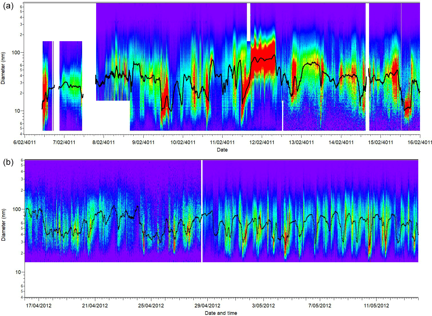
Figure 1 Time series of aerosol size distribution for SPS-I (a) and SPS-II (b). The black line on each plot is the mode diameter. Contour plots were produced using SMPS Loading and Processing Functions version 1.8.8 authored by Tim Onasch from Aerodyne Research, Inc.

3.1.2 Aerosol scattering coefficient

During SPS-I and SPS-II aerosol scattering was measured at 525 nm using an integrating nephelometer (Ecotech Aurora 1000G). In this instrument, air is drawn into a chamber with a light beam at 525 nm and a photomultiplier detector set at right angles to the light beam. Particles in the air scatter the light beam. The detector measures the scattered light beam in the forward and backward directions. The nephelometer was operated according to the Australian standard method for an integrated nephelometer (AS/NZS 3580.12.1:2015, 2015). The inlet to the nephelometer was heated to ensure the relative humidity of the sample stream was less than 40 %. Daily zero air and span gas checks were carried out and the nephelometer was calibrated using CO₂ every 3 months. The estimated uncertainty listed in Table 1 was determined from the propagation of relative uncertainty in the calibration gas accuracy and uncertainties in humidity, temperature, and pressure measurements specified in AS/NZS 3580.12.1:2015 (2015). Figure 2 shows the time series of aerosol scattering coefficient during SPS-I and SPS-II.

Figure 2 Time series of hourly averaged aerosol scattering coefficients during SPS-I (a) and SPS-II (b).

3.1.3 PM₁₀

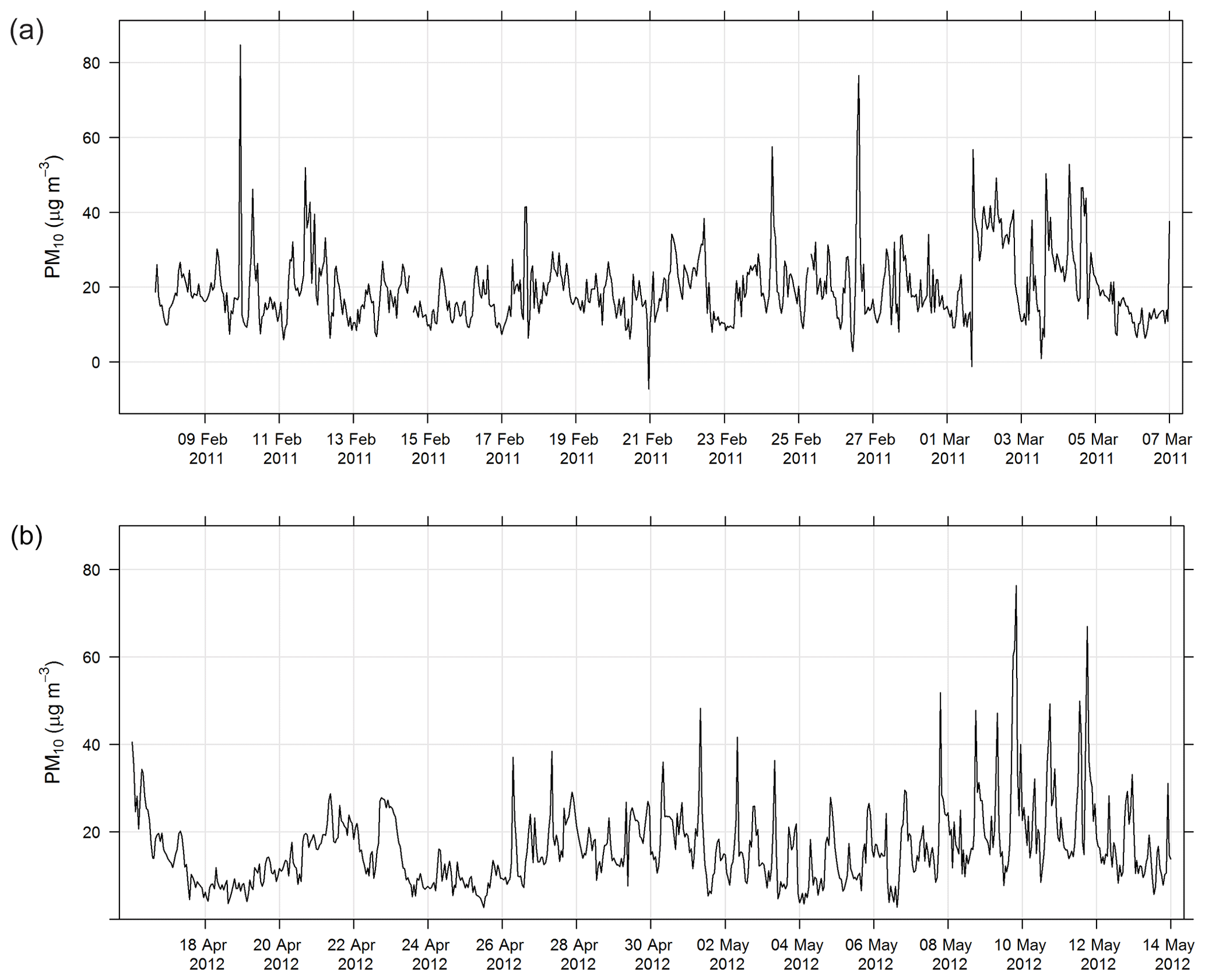
During SPS-I and SPS-II the concentration of PM₁₀ was measured using a tapered element oscillating microbalance (Thermo TEOM1405). Air was drawn through a PM₁₀ impactor and a filter sitting on an oscillating microbalance. As mass loaded onto the filter, the frequency of oscillation changed and mass was recorded. The inlet to the TEOM was heated to 50 ^∘C and the TEOM was operated according to Australian standards for PM₁₀ continuous direct mass using a tapered element oscillating microbalance analyser (AS/NZ 3580.9.8-2008, 2008). The estimated uncertainty listed in Table 1 was determined from the propagation of relative uncertainties for flow rates, temperature, mass flow controllers, and standard filter mass accuracy specified in AS/NZ 3580.9.8-2008 (2008). Figure 3 shows the time series of PM₁₀ during SPS-I and SPS-II.

Figure 3 Time series of hourly averaged PM₁₀ concentrations during SPS-I (a) and SPS-II (b).

3.1.4 Proton-transfer-reaction mass spectrometer

Proton-transfer-reaction mass spectrometry (PTR-MS) is a chemical ionization mass spectrometry technique capable of quantifying volatile organic compounds (VOCs) in a gaseous sample at time resolutions down to a fraction of a second. The major constituents of air, oxygen, nitrogen, etc. are not detected. PTR-MS is suitable for the measurement of a range of atmospheric VOCs including aromatics, oxygenates, organo-sulfurs, and terpenes.

The PTR-MS instrument operates with the aid of a custom-built auxiliary rack that regulates the flow of air in the sample inlet and controls whether the PTR-MS instrument is sampling ambient or zero air or calibration gas. During this study zero readings and calibrations against certified gas standards were performed on the PTR-MS instrument several times per day. Four calibration standards were used during the study, diluted to atmospheric concentrations using a set of mass flow controllers and a mixing chamber in the auxiliary rack. The PTR-MS instrument was calibrated for formaldehyde, acetaldehyde, acrolein, methacrolein, acetone, methyl ethyl ketone, methanol, ethyl acetate, benzene, xylene, trimethyl benzene, isoprene, a-pinene, 1,8 cineole, dimethyl sulfide, acetonitrile, and the mono-, di-, and trichlorobenzenes. Only m∕z values that were detected above the method detection limit (MDL) greater than 25 % of the time, and had peak-to-noise ratios greater than 5 (95th percentile/MDL), were reported.  Further details are available in Galbally et al. (2007) and Dunne et al. (2012, 2018). The estimated uncertainty listed in Table 1 was taken from Dunne et al. (2018). The time series of benzene, α-pinene, and formaldehyde measured during SPS-I and SPS-II are shown in Figs. 4 and 5.

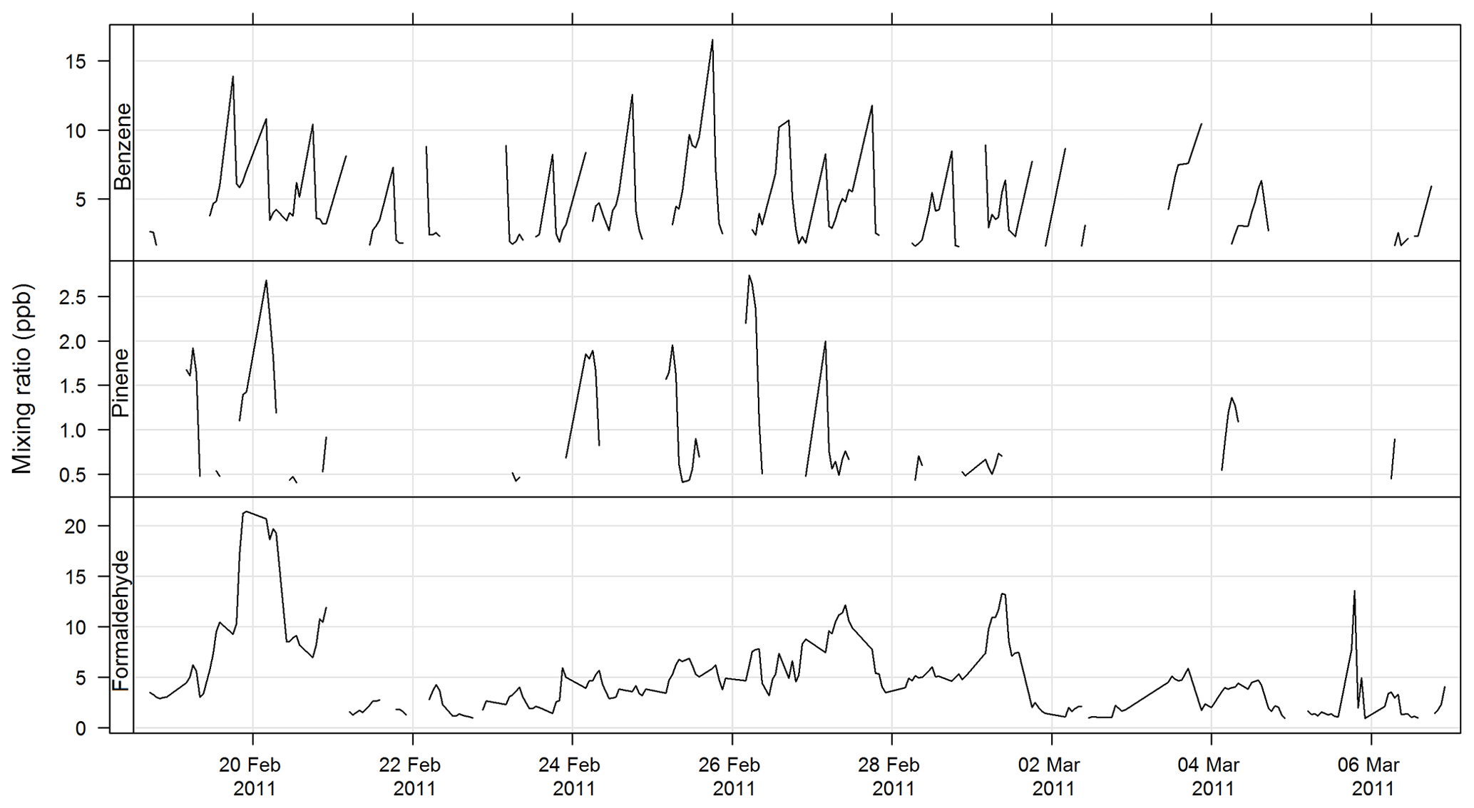
Figure 4 Time series of ambient benzene, α-pinene, and formaldehyde mixing ratios during SPS-I measured with the PTR-MS instrument.

Figure 5 Time series of ambient benzene, α-pinene, and formaldehyde mixing ratios during SPS-II measured with the PTR-MS instrument.

3.1.5 Radon

Radon concentration was measured using a dual-flow-loop two-filter detection method (Whittlestone and Zahorowski, 1998; Chambers et al., 2014). The detector used for SPS-I and SPS-II was a 700 L model, which sampled at 40 L min⁻¹ from 2 m above ground level (45 min response time, 40–50 mBq m⁻³ lower detection limit). Operation followed the approach described by Chambers et al. (2011). An on-site calibration was carried out using a NIST traceable Pylon Ra-226 source (118.19±4 % kBq), and instrumental background checks were carried out pre- and post-deployment.

In addition to the raw detector output, a time series of the atmospheric radon concentration was computed by deconvolving the detector output, thereby correcting for the slow detector response (Griffiths et al., 2016). The deconvolved time series has larger statistical uncertainty than the uncorrected detector output, but is a better representation of the atmospheric radon concentration during periods when it is changing rapidly (e.g. during the morning transition between nocturnal and convective boundary layers). Figure 6 shows the time series of radon measured during SPS-I and SPS-II.

Figure 6 Time series radon concentrations during SPS-I and SPS-II.

3.1.6 Criteria gases

Carbon monoxide (CO) was measured using a nondispersive infrared CO analyser (Ecotech ML9830 CO trace gas analyser). In this instrument, sample air is drawn into a cell where a beam of infrared light is passed through it to a photodetector. The amount of light absorbed by CO in the sample is proportional to the number of molecules present, and the concentration of CO is determined by comparing the intensity of light measured by the photodetector with a cell containing a reference gas. The CO analyser was operated according to the Australian standard method for the determination of CO with a direct-reading instrumental method (AS/NZS 3580.7.1:2011, 2011). The estimated uncertainty listed in Table 1 is taken from AS/NZS 3580.7.1:2011 (2011).

Oxides of nitrogen were measured using a chemiluminescent analyser (Ecotech EC9841 NO_x trace gas analyser). In this instrument, nitric oxide (NO) in the sample air reacts with ozone (produced from an ultraviolet light) within a reaction chamber, producing chemiluminescence in the wavelength range 600–3000 nm. The concentration of NO is proportional to the light intensity measured by a photomultiplier tube. In a second sample stream, total nitrogen oxides (NO_x) are reduced to NO using a selective converter. The concentration of nitrogen dioxide (NO₂) is assumed to be the difference between total NO_x and NO. The analyser was operated according to the Australian standard method for the determination of oxides of nitrogen with a direct-reading instrumental method (AS/NZS 3580.5.1:2011, 2011). The estimated uncertainty listed in Table 1 is taken from AS/NZS 3580.5.1:2011 (2011).

Ozone (O₃) was measured using an ultraviolet spectrometer (Ecotech EC9810). In this instrument, a beam of ultraviolet light is passed through the sample air within a cell containing an ultraviolet detector. The amount of light absorbed in the sample is proportional to the number of O₃ molecules present and the decrease in light intensity determines the O₃ concentration in the sample. The analyser was operated according to the Australian standard method for the determination of O₃ with a direct-reading instrumental method (AS/NZS 3580.6.1:2011, 2011). The estimated uncertainty listed in Table 1 is taken from AS/NZS 3580.6.1:2011 (2011).

Sulfur dioxide (SO₂) was measured by a pulsed fluorescence spectrophotometer (Ecotech EC9850). A stream of sample air is drawn through a cell where it is exposed to pulsed ultraviolet light, resulting in excitation of SO₂ molecules. These molecules subsequently fluoresce, by re-emitting light at a different wavelength. The intensity of the fluorescent light measured by a photomultiplier tube is proportional to the concentration of SO₂ in the sample air. The analyser was operated according to the Australian standard method for the determination of SO₂ with a direct-reading instrumental method (AS/NZS 3580.4.1:2008, 2008). The estimated uncertainty listed in Table 1 is taken from AS/NZS 3580.4.1:2008 (2008).

The time series for CO, NO_x, O₃, and SO₂ for SPS-I and SPS-II are shown in Figs. 7 and 8.

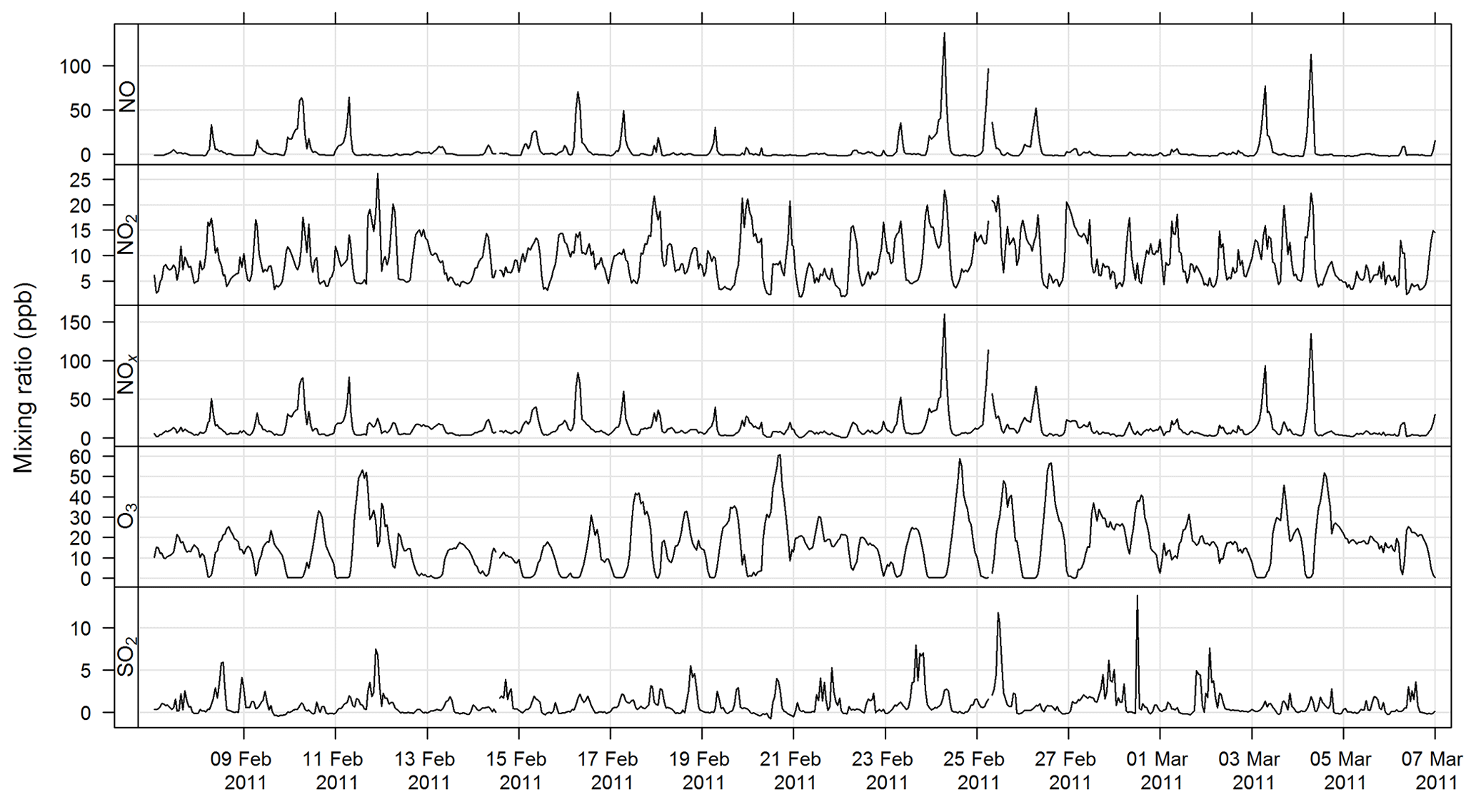
Figure 7 Time series of hourly averaged mixing ratios of criteria gases NO, NO₂, NO_x, O₃, and SO₂ during SPS-I.

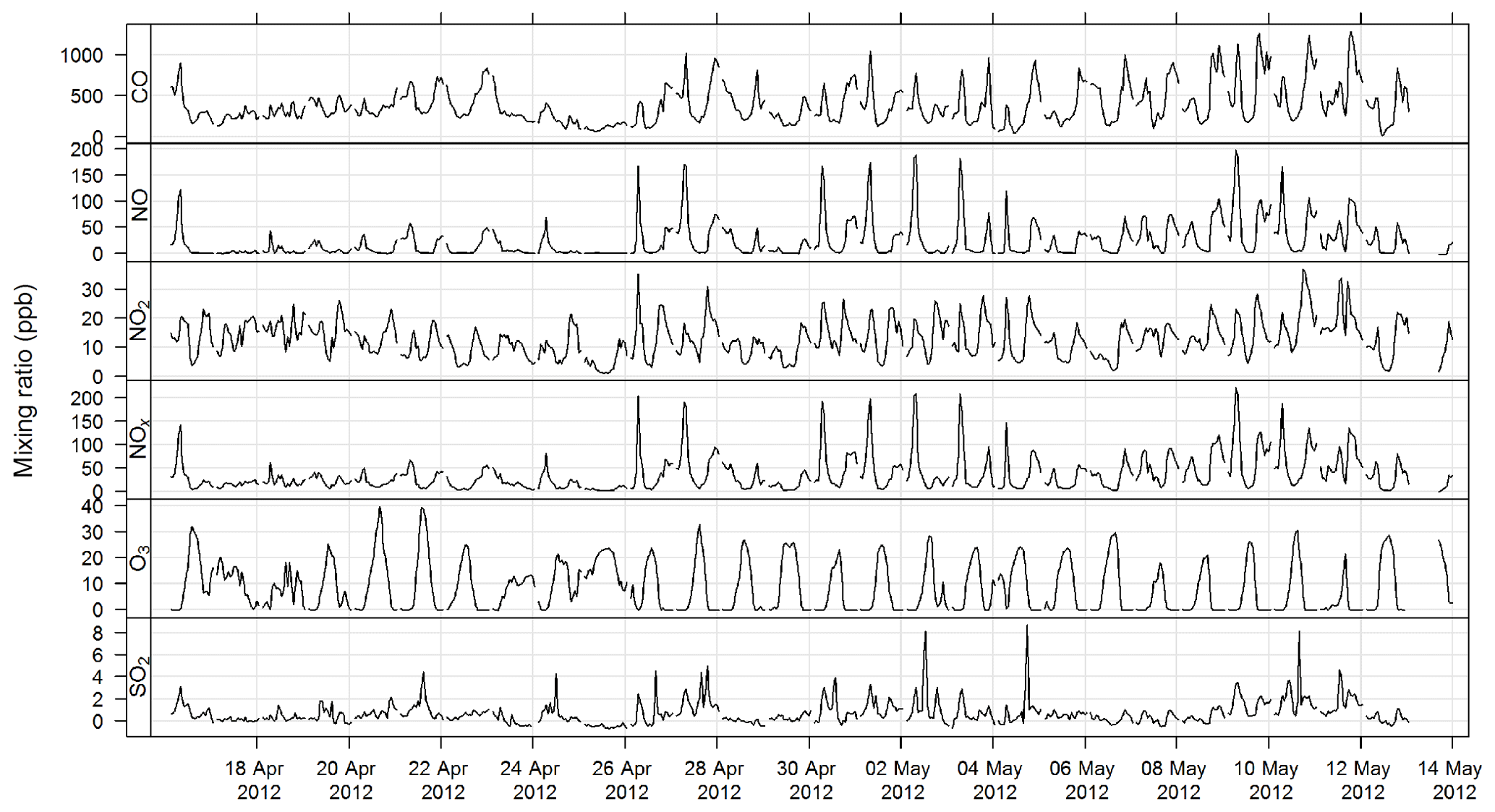
Figure 8 Time series of hourly averaged mixing ratios of criteria gases CO, NO, NO₂, NO_x, O₃, and SO₂ during SPS-II.

3.1.7 Meteorology

An ultrasonic sensor (Met One MET505) was used to measure wind speed and wind direction. Temperature and relative humidity were measured using a temperature and humidity probe (Vaisala HMP 155). Solar radiation was measured using a pyranometer (Middleton 8536). All instruments were sited and operated according to the Australian standard method for meteorological monitoring for ambient air quality monitoring applications (AS/NZS 3580.14:2014, 2014). The estimated uncertainties listed in Table 1 are taken from AS/NZS 3580.14:2014 (2014).

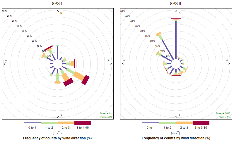
The time series of temperature and relative humidity are shown for SPS-1 in Fig. 9; in addition solar radiation is also shown for SPS-II in Fig. 10. The frequencies of wind speeds as a function of wind direction for SPS-I and SPS-II are shown in Fig. 11.

Figure 9 Time series of ambient temperature and relative humidity during SPS-I.

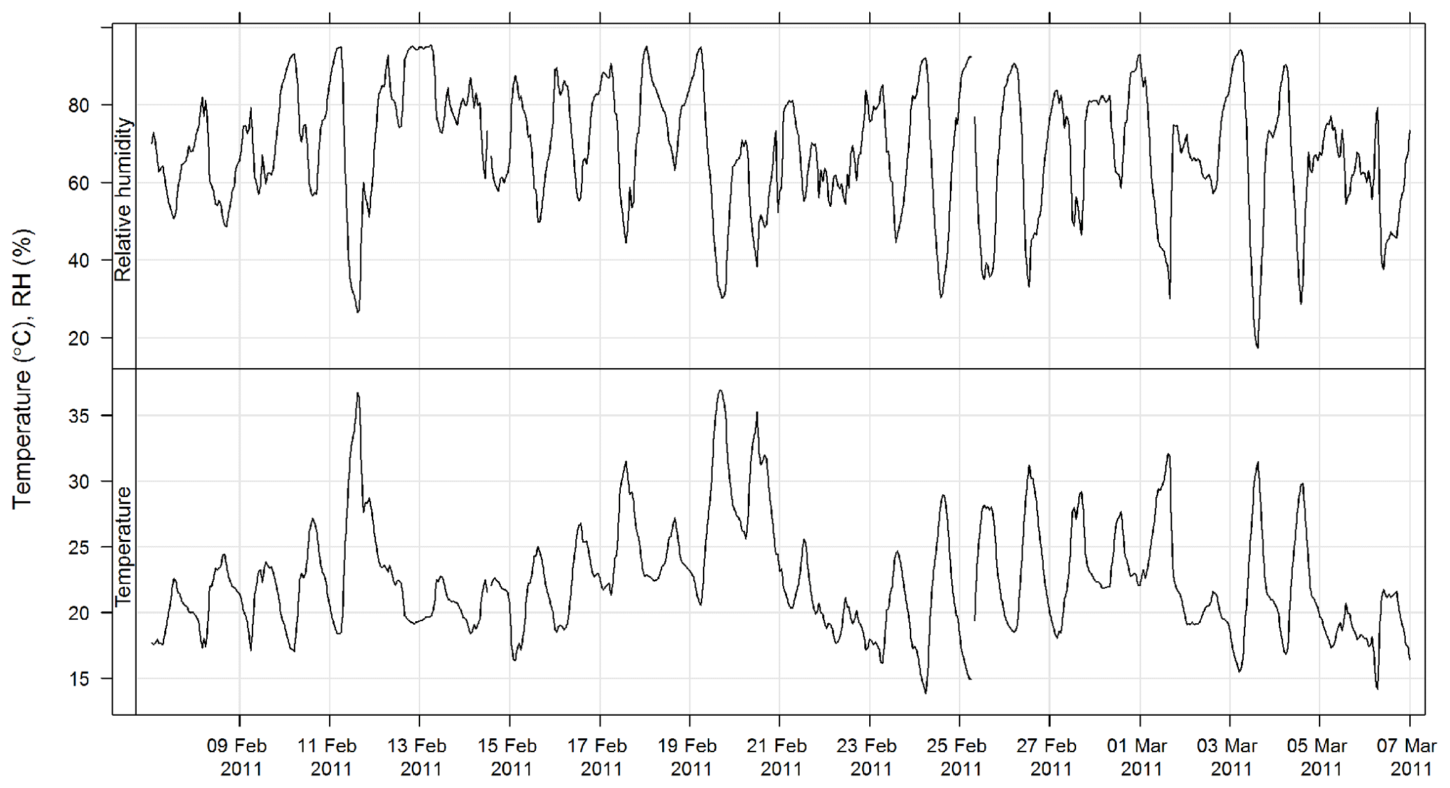
Figure 10 Time series of ambient temperature, relative humidity, and solar radiation during SPS-II.

Figure 11 Wind roses during SPS-I in 2011and SPS-II in 2012.

3.1.8 Lidar and boundary layer detection

A Leosphere ALS 450 lidar was used to estimate cloud base, cloud top (for optically thin clouds), and the height of the boundary layer. The lidar incorporated a 355 nm UV laser that scattered light in the column of air back to a receiver. Raw data have a spatial resolution of 15 m and a temporal resolution of 30 s covering a range from about 200 to 20 km. The physical basis for lidar remote sensing is described by Weitkamp (2005).

The conditions under which the lidar could determine the depth of the boundary layer included (1) the top of the boundary layer being deeper than about 200 m and (2) accompanied by a sudden decrease in aerosol concentration. These conditions were most often met during daylight hours with clear skies or some fair weather cumulus.

Two approaches were combined in order to filter out periods with ambiguous retrievals of the boundary layer depth. The first method was an automated method, called STRAT-2D (Haeffelin et al., 2012), which used the Canny edge detection algorithm to detect discontinuities in the backscatter signal as a function of time and range. It is implemented in the STRAT analysis toolkit (Morille et al., 2007). The second method was a manual technique, in which the boundary layer top was detected by visual identification of the inflection point in a plot of log (Sr²)∼r, where S is the received backscatter and r is the range from the lidar.

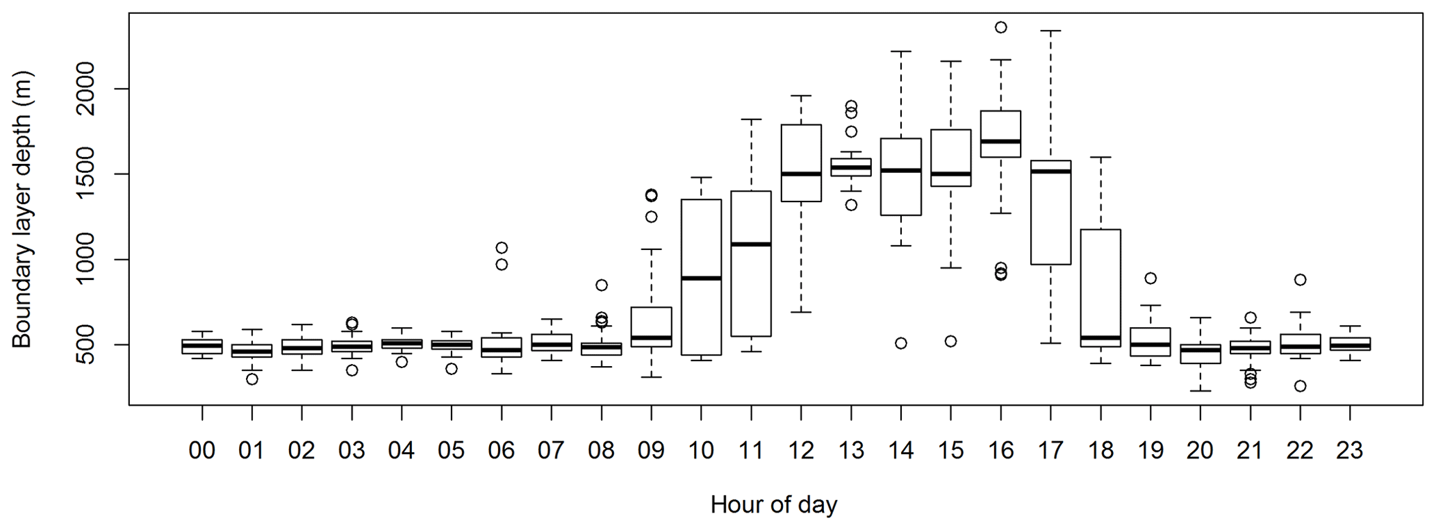
Based on the two estimates above, the boundary layer depth was computed by taking the average of the two estimates and assigning an uncertainty given by the range between the two estimates. Figure 12 shows the diurnal cycle in boundary layer depth measured during SPS-II.

Figure 12 Boundary layer depth as a function of hour of the day for SPS-II.

3.2 Integrated measurements

3.2.1 High-volume sampler

In both SPS-I and SPS-II aerosol samples were collected using an Ecotech 3000 high-volume sampler with a PM_2.5 size-selective inlet (flow rate 67.8 m³ h⁻¹ controlled with a mass flow controller, ambient temperature, and pressure monitored so that both the ambient volumetric and standard flow rates were determined). Quartz membrane filters (250 mm ×200 mm Pall tissue quartz p/n 7204 prebaked at 600 ^∘C for 4 h to reduce adsorbed organic vapours) were used to collect samples and were stored in a freezer within sealed containers before and after sampling.

Throughout the study field blank samples (five for SPS-I and nine for SPS-II) were collected by running a pre-baked filter in the high-volume sampler for 1 min. Filter handling and analysis procedures were consistent for the field blanks and sample filters. In addition, to correct for sampling artefacts on the organic carbon (OC) and elemental carbon (EC) concentrations, two filters were placed in the filter holder in sequence (front filter and back filter) for 20 of the SPS-I samples. The adsorption of volatile gases onto the filter material results in positive artefacts, while degassing of semi-volatile compounds from the collected aerosol on the front filter, which may then be absorbed onto the back filter, results in negative artefacts (Chow et al., 2010).

The filters were analysed for soluble ions using the method described in Sect. 3.3.1 and for OC and EC the method described in Sect. 3.3.3.

3.2.2 Low-volume sampler

PM_2.5 samples were collected using a sampler from the ANSTO Aerosol Sampling Program, which includes a PM_2.5 cyclone (flow rate 22 L min⁻¹). The cyclone is the same as that used in the U.S. EPA IMPROVE network (http://vista.cira.colostate.edu/Improve/, last access: 4 October 2019). Thin 25 mm stretched Teflon filters were used to collect samples coincidentally with the high-volume sampler to allow comparison of data during SPS-II. Samples were analysed for elemental concentrations using the method described in Sect. 3.3.2.

3.2.3 VOC and carbonyl sequencer

The VOC and carbonyl sequencer is an automatic continuous air sampler for sampling of VOC and carbonyls simultaneously. It has two channels: one for VOC and the other one for carbonyls. Each channel contains a sample inlet, nine sampling ports, four solenoid valves, and a sampling pump. A new sequencer was built for SPS-II that included a cooling system to keep the carbonyl tubes at 5–7 ^∘C as well as extra sampling ports.

Samples were collected three times per day (05:00–10:00, 11:00–19:00, and 19:00–05:00) and during SPS-I a field blank (unopened tube) was collected each day. The new sequencer used in SPS-II incorporated additional sampling ports that were used to load extra sampling tubes that did not have any air sampled through them. These were then used as field blanks. The tubes were analysed for VOC concentrations using the method described in Sect. 3.3.5 and for carbonyls using the method described in Sect. 3.3.4.

3.2.4 Acid–alkaline gas sampler

The acid–alkaline gas sampler drew air through a three-stage 47 mm filter pack at an ambient flow rate of 10 L min⁻¹. The first stage of the three-stage filter pack contained a Teflon filter (Millipore fluoropore p/n FALP04700) to remove particles from the air stream, the second stage contained a sodium-hydroxide-coated quartz filter (Pall tissue quartz p/n 7202) to trap acidic gases, and the final stage contained a citric-acid-coated quartz filter to trap alkaline gases. The filters were extracted in de-ionized water and analysed for soluble ion concentrations using the method described in Sect. 3.3.1.

3.3 Analysis methods

3.3.1 Ion chromatography

Suppressed ion chromatography (IC) and high-performance anion-exchange chromatography with pulsed amperometric detection (HPAEC-PAD) were used to measure water-soluble ions and anhydrous sugars including levoglucosan on a 6.25 cm² a portion of each quartz high-volume sampler filter. De-ionized water (10 mL of 18.2 mΩ) was used to extract the quartz filter portions, which were then preserved using 0.1 mL of chloroform. The acid and alkaline gas filter samples were also analysed by IC and the 47 mm filters were extracted in 3 mL of 18.2 mΩ de-ionized water and preserved with 0.03 mL of chloroform.

A Dionex ICS-3000 ion chromatograph was used to determine soluble ion (anion and cation) concentrations. The system included a Dionex AS17c analytical column (2×250 mm), an ASRS-300 suppressor, and a gradient eluent of 0.75 to 35 mM potassium hydroxide to separate the anions and a Dionex CS12a column (2×250 mm), CSRS-300 suppressor, and an isocratic eluent of 20 mM methanesulfonic acid to separate the cations. The species analysed were

• chloride (Cl⁻)

• nitrate (${\mathrm{NO}}_{\mathrm{3}}^{-}$)

• sulfate (${\mathrm{SO}}_{\mathrm{4}}^{\mathrm{2}-}$)

• oxalate (${\mathrm{C}}_{\mathrm{2}}{\mathrm{O}}_{\mathrm{4}}^{-}$)

• formate (HCOO⁻)

• acetate (CH₃COO⁻)

• phosphate (${\mathrm{PO}}_{\mathrm{4}}^{\mathrm{3}-}$)

• methanosulfonate (MSA⁻)

• sodium (Na⁺)

• ammonium (${\mathrm{NH}}_{\mathrm{4}}^{+}$)

• magnesium (Mg²⁺)

• calcium (Ca²⁺)

• potassium (K⁺).

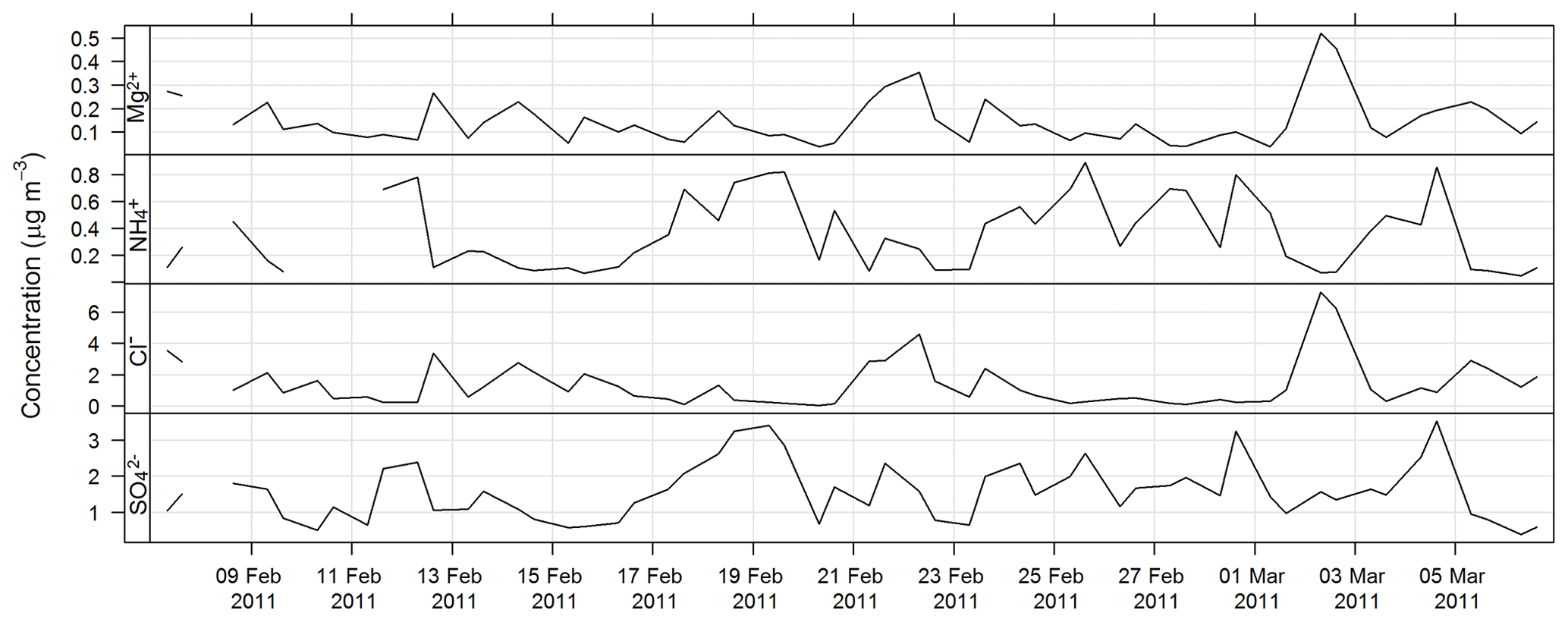
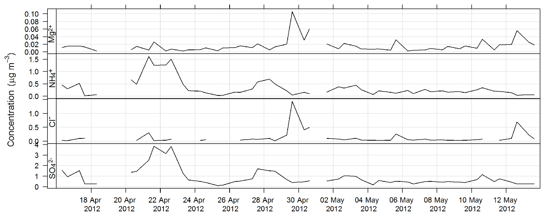
The estimated uncertainty listed in Table 1 was determined from the propagation of relative uncertainty associated with the collection of samples on the high-volume sampler and the analytical method described here. The time series for Mg²⁺, Cl⁻ ${\mathrm{NH}}_{\mathrm{4}}^{+}$, and ${\mathrm{SO}}_{\mathrm{4}}^{\mathrm{2}-}$ during SPS-I are shown in Fig. 13 and those during SPS-II in Fig. 14.

Figure 13 Time series of Mg²⁺, Cl⁻ ${\mathrm{NH}}_{\mathrm{4}}^{+}$, and ${\mathrm{SO}}_{\mathrm{4}}^{\mathrm{2}-}$ during SPS-I in 2011.

Figure 14 Time series of Mg²⁺, Cl⁻ ${\mathrm{NH}}_{\mathrm{4}}^{+}$, and ${\mathrm{SO}}_{\mathrm{4}}^{\mathrm{2}-}$ during SPS-II in 2012.

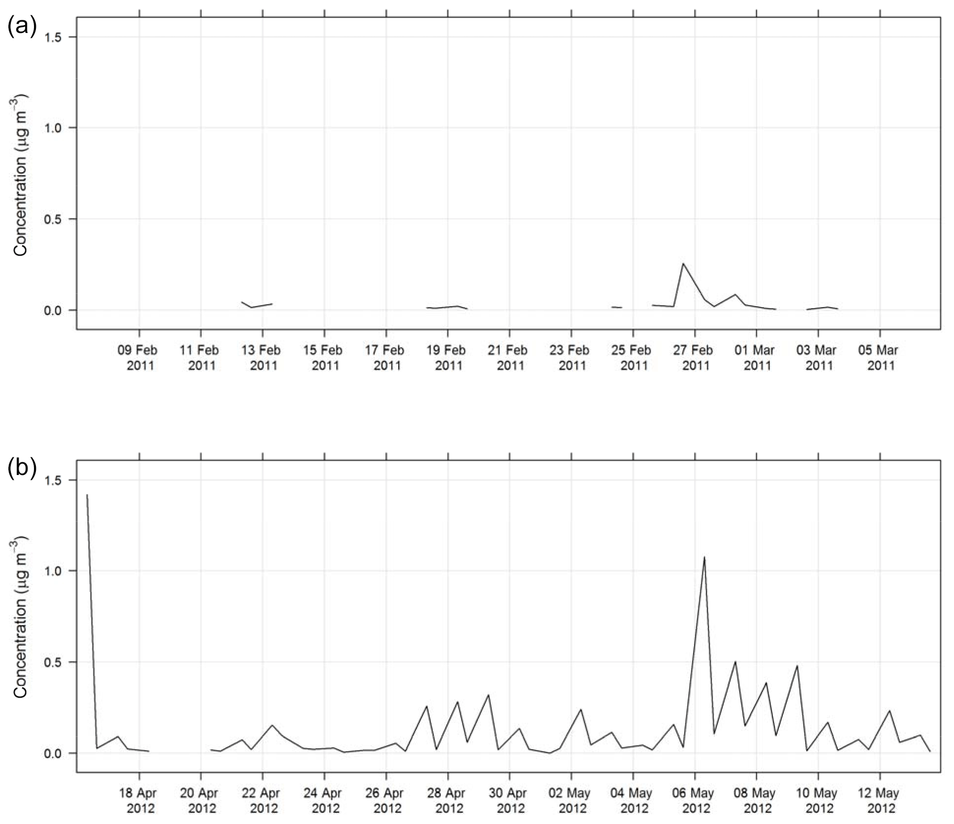
An HPAEC-PAD with a Dionex ICS-3000 chromatograph with electrochemical detection was used to determine anhydrous sugar concentrations. The system was operated in the integrating (pulsed) amperometric mode using the carbohydrate (standard quad) waveform and utilizing disposable gold electrodes. A Dionex CarboPac MA1 analytical column (4 mm × 250 mm) with a gradient eluent of 300 to 550 mM sodium hydroxide was used to separate the anhydrous sugars (Iinuma et al., 2009). The species analysed were levoglucosan (C₆H₁₀O₅, an anhydrous sugar – woodsmoke tracer) and mannosan (C₆H₁₀O₅, an anhydrous sugar – woodsmoke tracer). The time series of levoglucosan during SPS-I and SPS-II are shown in Fig. 15.

Figure 15 Time series of levoglucosan concentrations during SPS-I (a) and SPS-II (b).

3.3.2 Ion beam analysis

Nuclear ion beam analysis (IBA) techniques employing the nondestructive ANSTO STAR 2MV accelerator were used to determine the concentration of elements on the 25 mm Teflon filters collected by the low-volume sampler. Analysis of aluminium to lead was carried out using proton-induced X-ray emission (PIXE; see Cohen, 1993, for details), analysis of light elements such as fluorine and sodium was carried out by proton-induced gamma-ray emission (PIGE; see Cohen, 1998, for details), and analysis of hydrogen was carried out using proton elastic scattering analysis (PESA; see Cohen et al., 1996 for details). Uncertainties reported in Cohen et al. (1996) include ±14 % for sodium, ±10 % for silicon, and ±7 % for hydrogen.

The elements determined were

• hydrogen (H)

• sodium (Na)

• aluminium (Al)

• silicon (Si)

• phosphorous (P)

• sulfur (S)

• chlorine (Cl)

• potassium (K)

• calcium (Ca)

• titanium (Ti)

• vanadium (V)

• chromium (Cr)

• manganese (Mn)

• iron (Fe)

• cobalt (Co)

• nickel (Ni)

• copper (Cu)

• zinc (Zn)

• bromine (Br)

• lead (Pb).

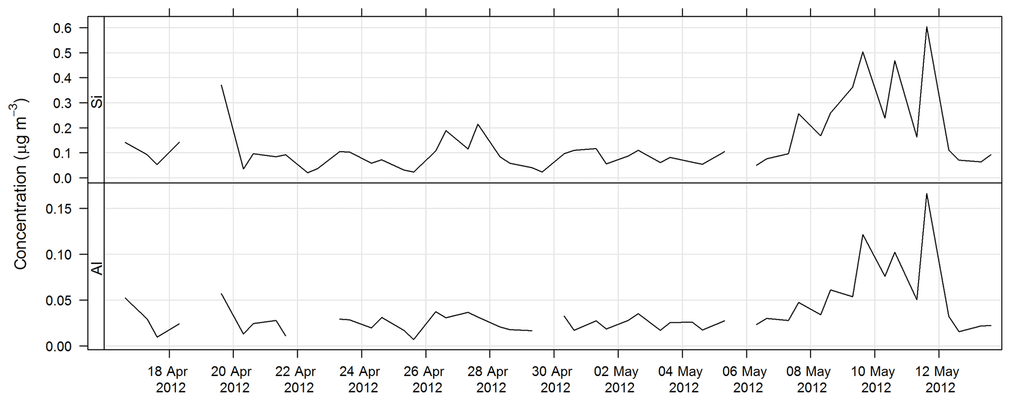
The time series of Al and Si for SPS-II are shown in Fig. 16.

Figure 16 Time series of Al and Si during SPS-II.

3.3.3 Organic carbon and elemental carbon analysis

A Desert Research Institute model 2001A thermal–optical carbon analyser was used to determine the concentration of elemental carbon (EC) and organic carbon (OC) on a portion of the quartz filters collected using a PM_2.5 high-volume sampler. The IMPROVE-A temperature protocol (Chow et al., 2007) was employed and included using laser reflectance to correct for charring. Before analysis the oven was baked to 910 ^∘C for 10 min to remove residual carbon and system blank levels were then tested until <0.20 µg C cm⁻² was reported (with repeat oven baking if necessary). Calibration checks were performed twice daily to monitor possible catalyst degeneration. The analyser is reported to measure carbon concentrations between 0.05 and 750 µg C cm⁻², with uncertainties in OC and EC of ±10 %.

Figure 17 Time series of OC and EC during SPS-I in 2011.

Figure 18 Time series of OC and EC during SPS-II in 2012.

Four OC fractions at four non-oxidizing heat ramps (OC1 =140 ^∘C, OC2 =280 ^∘C, OC3 =480 ^∘C, OC4 =580 ^∘C) and three EC fractions at three oxidizing heat ramps (EC1 =580 ^∘C, EC2 =740 ^∘C, EC3 =840 ^∘C) are measured in the IMPROVE-A carbon method. The sum of the different OC fractions and the OCpyro (the OC that was pyrolysed and was measured from the reflectance of the filter) determined total OC. The sum of the EC fractions minus OCpyro determined total EC.

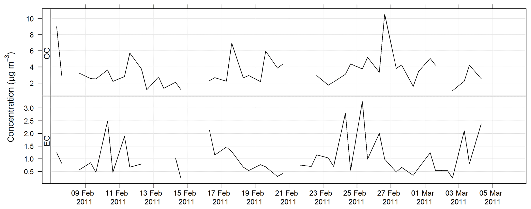
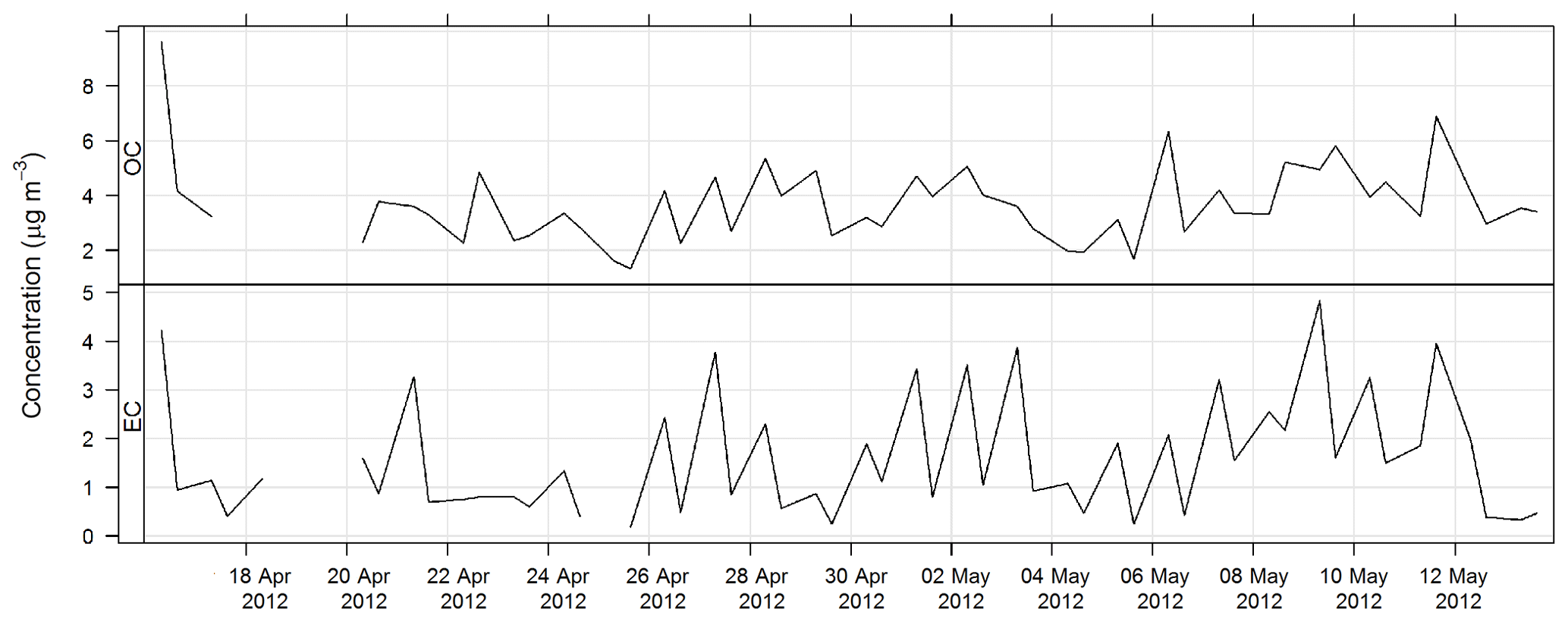
The time series for OC and EC during SPS-I are shown in Fig. 17 and the time series for OC and EC during SPS-II are shown in Fig. 18.

3.3.4 Carbonyls analysis

Carbonyls were collected by the sequencer onto cartridges (Supelco LpDNPH S10 p/n 21014) containing high-purity silica adsorbent coated with 2,4-dinitrophenylhydrazine (DNPH), where they were converted to the hydrazone derivatives. Samples were refrigerated immediately after sampling until analysis. The derivatives were extracted from the cartridge in 2.5 mL of acetonitrile and analysed by high-performance liquid chromatography (HPLC) with diode array detection (DAD). The DAD enables the absorption spectra of each peak to be determined. The difference in the spectra highlights which peaks in the chromatograms are mono- or dicarbonyl DNPH derivatives and, along with retention times, allows the identification of the dicarbonyls glyoxal and methylglyoxal. Further details of this method can be found in Lawson et al. (2015). The estimated uncertainty listed in Table 1 was taken from Dunne et al. (2018). The time series of methylglyoxal and formaldehyde for SPS-I is shown in Fig. 19 and time series of methylglyoxal and formaldehyde during SPS-II are shown in Fig. 20.

Figure 19 Time series of ambient formaldehyde and methylglyoxal mixing ratios during SPS-I.

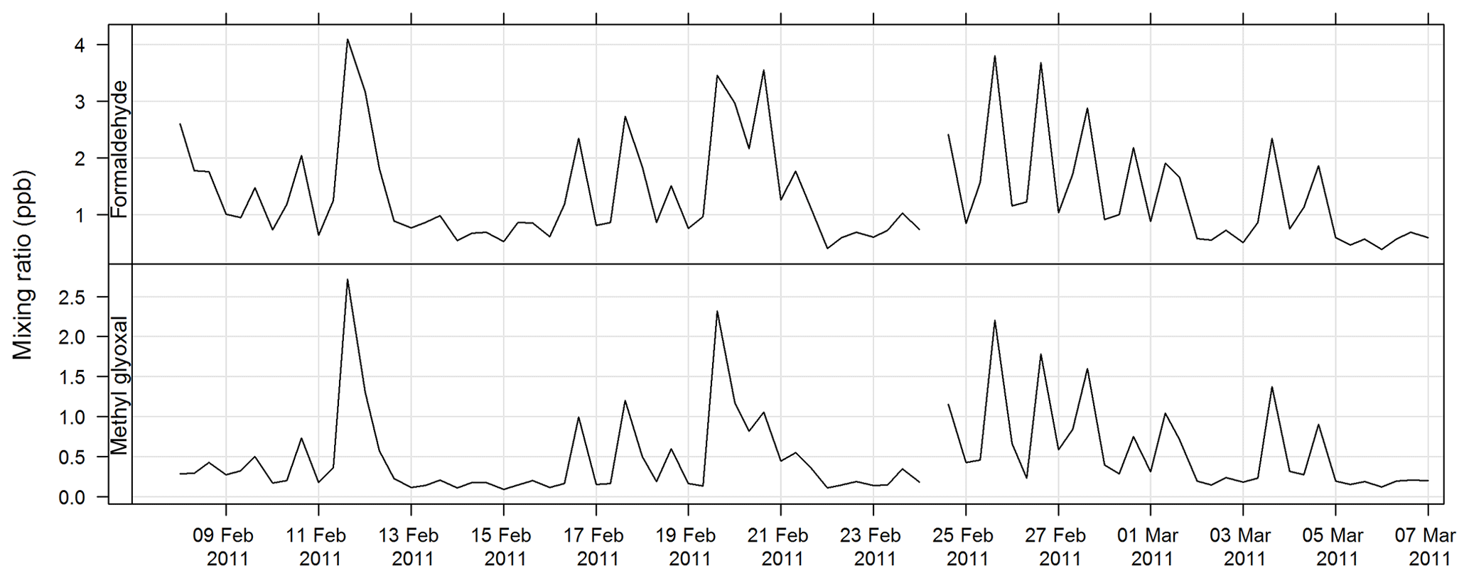
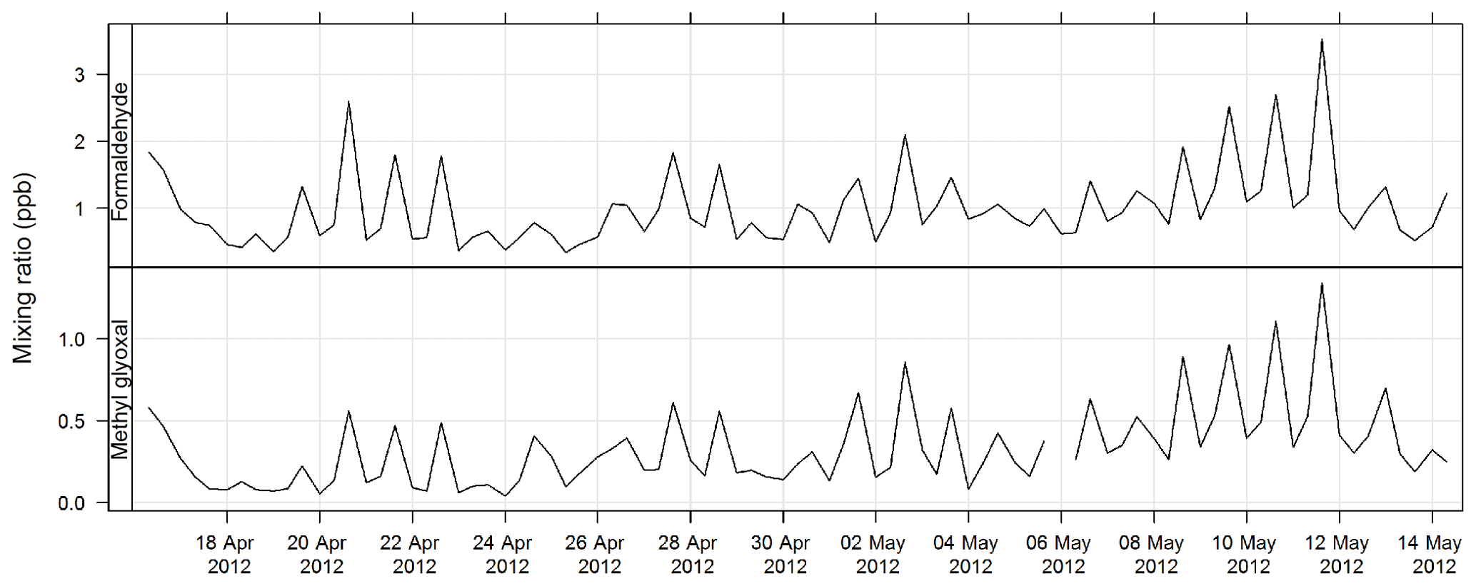
Figure 20 Time series of ambient formaldehyde and methylglyoxal mixing ratio concentrations during SPS-II.

3.3.5 Volatile organic compound analysis

An automatic volatile organic compound (VOC) sampler was used to collect VOC samples by actively drawing air through two adsorbent tubes in series (Markes Carbograph 1TD/Carbopack X), which were then analysed by a PerkinElmer TurboMatrix^™ 650 ATD (automated thermal desorber) and a Hewlett Packard 6890A gas chromatograph (GC) equipped with a flame ionization detector (FID) and a mass selective detector (MSD). Calibration was via certified BTEX (benzene, toluene, ethylbenzene, and xylenes), TO 15/17, terpenes, alcohols, and PAM gas standards (Cheng et al., 2016). The method of AT (adsorbent tube) VOC sampling and analysis in this study was compatible with ISO16017-1:2000 (ISO 2000) and according to U.S. EPA Compendium method TO-17 (USEPA TO-17). The estimated uncertainty listed in Table 1 was taken from Dunne et al. (2018). The time series for total alkane, aromatic, and terpene concentrations for SPS-I are shown in Fig. 21 and for SPS-II in Fig. 22.

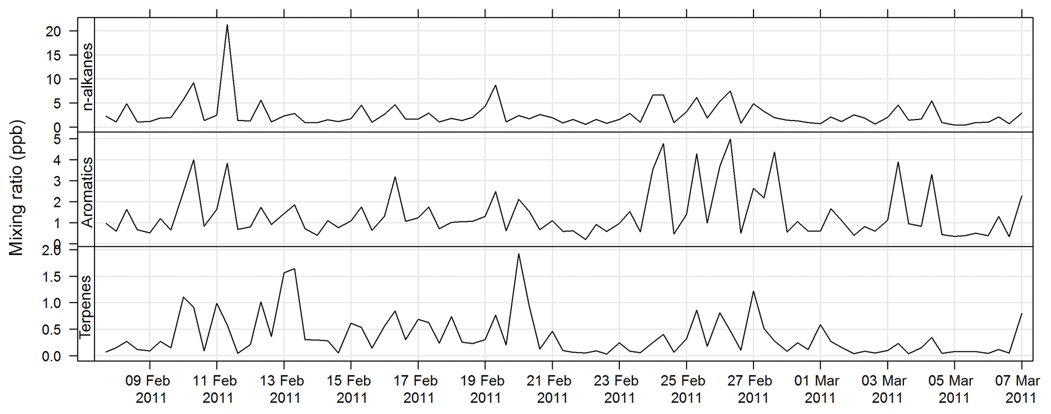
Figure 21 Time series of total alkane, total aromatics, and total terpene mixing ratios during SPS-I in 2011 measured on absorbent tubes.

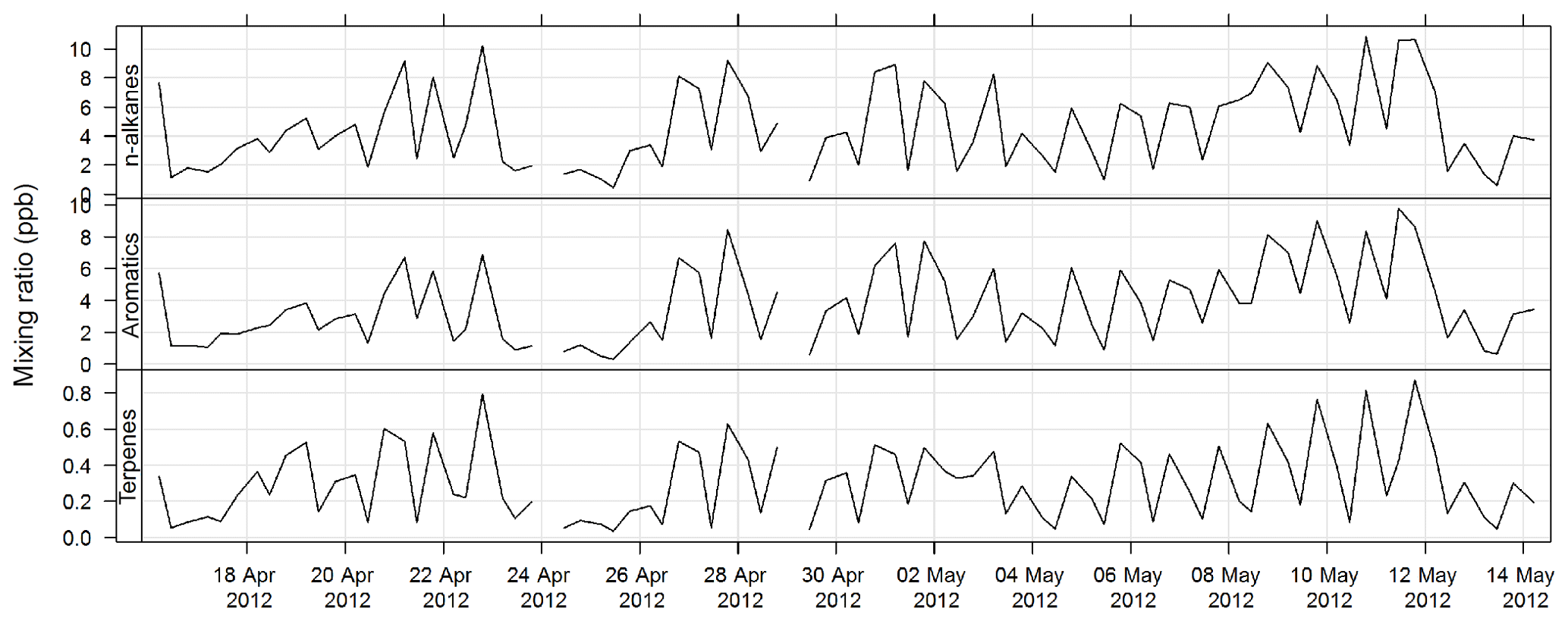
Figure 22 Time series of total alkane, total aromatics, and total terpene mixing ratios during SPS-II in 2012 measured on absorbent tubes.

4 Data availability

The data sets for both SPS-I and SPS-II are stored on the Commonwealth Scientific and Industrial Research Organisation (CSIRO) data access portal. The SPS-I data set is available at Keywood et al. (2016a, https://doi.org/10.4225/08/57903B83D6A5D) and the SPS-II data set is available at Keywood et al. (2016b, https://doi.org/10.4225/08/5791B5528BD63).

5 Aerosol composition

The factors that determine the composition of aerosols are the source of the aerosols (or precursor gases) and subsequent transformations that occur in the atmosphere or within the aerosol themselves. As such the sources of aerosols may be inferred from the chemical composition of the aerosol samples. A detailed analysis of the aerosol composition data is beyond the scope of a paper in this journal. Instead, presented here are the data for some species that can be used as markers for different aerosol sources.

Table 2 lists the markers that can be used to trace different aerosol sources. In some instances, a chemical species is a unique tracer for a source. For example, levoglucosan is a unique tracer for biomass burning (Simoneit et al., 1999; Simoneit, 2002). The time series of levoglucosan for both sampling periods is shown in Fig. 15. Concentrations were generally greater in SPS-II than SPS-I, indicating a greater contribution of biomass burning, most likely wood heaters used for domestic heating during autumn in Sydney in SPS-II.

Table 2 Sources and their indicator species.

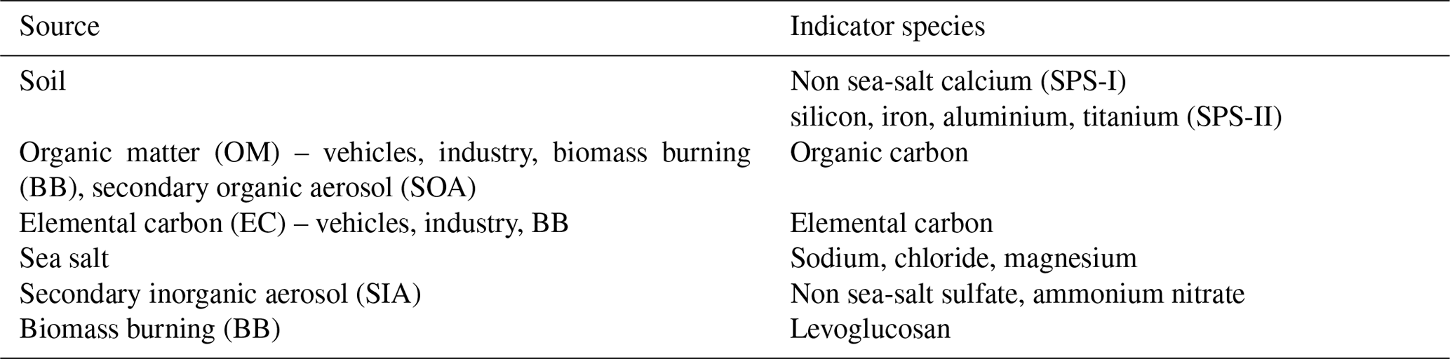
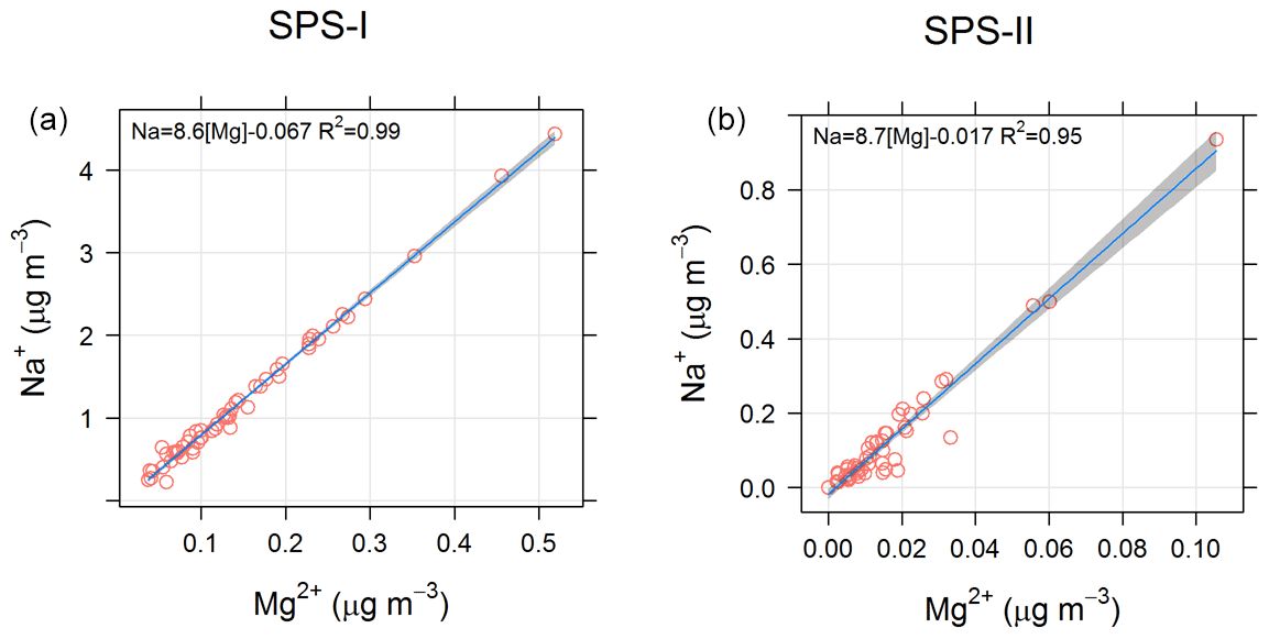
In addition the ratios of different species may provide information about an aerosol source. For example a sea-salt source may be indicated by a [${\mathrm{Na}}^{+}/{\mathrm{Mg}}^{\mathrm{2}+}$] ratio close to 8.3 (Millero et al., 2008), and an Australian crustal dust source may be indicated by a [Si∕Al] ratio of close to 3.08 (Radhi et al., 2010). Figure 23 shows the relationship between Na⁺ and Mg²⁺ for SPS-I and SPS-II, suggesting that the ratio of these species is close to that of sea salt. Figure 24 shows the relationship between Si and Al for SPS-II. The slope of 4 shown in the regression line is similar to that measured by Radhi et al. (2010), indicative of Australian dusts.

Figure 23 Scatter plot of Mg and Na for SPS-1 (a) and SPS-II (b).

Many compounds, however, may be derived from more than one source (e.g. EC can be present in vehicle emissions, industrial emissions, and biomass burning), and when sufficient sample numbers allow (generally more than 100) receptor modelling methodologies can be used to apportion sources to the aerosol loadings (Norris et al., 2008). During both SPS-I and SPS-II 30 samples were collected in the mornings and 30 in the afternoons. Hence with only 60 samples for each sampling period, we are restricted to a qualitative and rudimentary assessment of aerosol sources utilizing information on relationships between some key marker species and the timing of their occurrence.

The time series for EC, OC, ${\mathrm{SO}}_{\mathrm{4}}^{\mathrm{2}-}$, Mg²⁺, and Ca²⁺ are shown above. The average concentrations for SPS-I and SPS-II for each of these species are shown in Fig. 25. A marker for sea salt, Mg²⁺, and a marker for soil, non sea-salt Ca²⁺, show higher concentrations during SPS-I (summer). Higher non sea-salt sulfate concentrations during SPS-1 (summer), a marker for secondary aerosol during summer, may indicate greater secondary aerosol production during summer. Levoglucosan (the marker for woodsmoke) and EC show the highest concentrations during SPS-II (autumn). The average OC concentration is not significantly different between SPS-I and SPS-II.

Figure 24 Scatter plot of Al and Si for SPS-II.

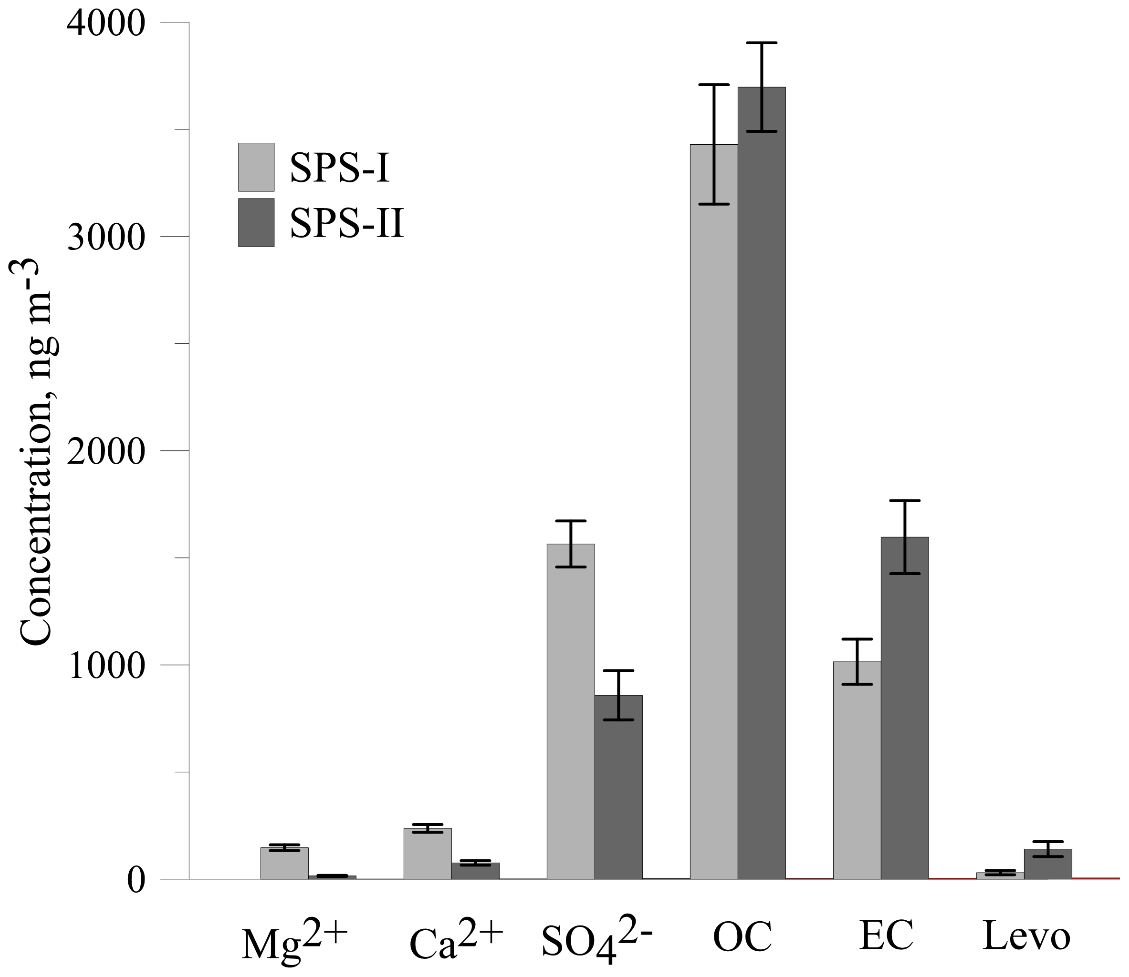
Figure 25 Comparison of average concentrations of Mg²⁺ (a marker for sea-salt), Ca (a marker for soil), ${\mathrm{SO}}_{\mathrm{4}}^{\mathrm{2}-}$ (a marker for secondary aerosol), OC, EC and levo = levoglucosan (biomass burning marker) during SPS-I and SPS-II. Error bars represent standard error (standard deviation/square root of number of observations). Mg²⁺, Ca²⁺, and ${\mathrm{SO}}_{\mathrm{4}}^{\mathrm{2}-}$ are significantly greater during SPS-I (p≪0.05), OC is not significantly different between SPS-I and SPS-II (p=0.4), EC and levoglucosan are significantly greater during SPS-II (p=0.003 EC and p=0.004 levoglucosan).

Higher sea salt and soil marker species in summer than autumn may be due to higher wind speeds observed during SPS-I since both sea salt and dust are mechanically produced aerosol. Figure 11 also showed there to be a greater recent oceanic fetch in summer; and during summer soils in rural regions are drier, and covered with less vegetation, so therefore more mobile. Higher secondary aerosol marker species in summer may indicate more photochemical aerosol production in summer, while higher biomass burning marker species in autumn may represent a greater contribution from wood heaters to the aerosol loading during this time of the year. Converse to the higher wind speeds during summer, the lower wind speeds during autumn are conducive to the build-up of pollutants during autumn which will also influence the concentrations of EC and levoglucosan during autumn. As noted above, a quantitative assessment of aerosol sources influencing the airshed during SPS-I and SPS-II could be carried out using a receptor modelling approach if more samples had been collected.