Global distribution of nearshore slopes with implications for coastal retreat

Nearshore slope, defined as the cross-shore gradient of the subaqueous profile, is an important input parameter which affects hydrodynamic and morphological coastal processes. It is used in both local and large-scale coastal investigations. However, due to unavailability of data, most studies, especially those that focus on continental or global scales, have historically adopted a uniform nearshore slope. This simplifying assumption could however have far-reaching implications for predictions/projections thus obtained. Here, we present the first global dataset of nearshore slopes with a resolution of 1 km at almost 620 000 points along the global coastline. To this end, coastal profiles were constructed using global topo-bathymetric datasets. The results show that the nearshore slopes vary substantially around the world. An assessment of coastline recession driven by sea level rise (SLR) (for an arbitrary 0.5 m SLR) with a globally uniform coastal slope of 1 : 100, as carried out in previous studies, and with the spatially variable coastal slopes computed herein shows that, on average, the former approach would underestimate coastline recession by about 40 %, albeit with significant spatial variation. The final dataset has been made publicly available at https://doi.org/10.4121/uuid:a8297dcd-c34e-4e6d-bf66-9fb8913d983d (Athanasiou, 2019).

1 Introduction

A total of 10 % of the world's population lives in low-lying coastal areas, i.e., less than 10 m above the current mean sea level (MSL) (McGranahan et al., 2007). In the future, the population density in these areas is expected to increase even more due to high rates of population growth and urbanization (Neumann et al., 2015). At the same time, coastal areas are exposed to a number of marine hazards that can lead to flooding or erosion. As the coastline comprises various different landforms (e.g., sandy coasts, rocky cliffs) and land uses (e.g., heavily urbanized or natural), the response to these hazards can vary significantly both spatially and temporally. One of the most vulnerable coastal types is sandy coasts, which are highly dynamic and can change in response to extreme marine events (McCall et al., 2010), long-term trends in MSL (Zhang et al., 2004), natural gradients in alongshore sediment transport (Antolínez et al., 2018), or human interventions (Giardino et al., 2018a; Luijendijk et al., 2018; Mentaschi et al., 2018).

Local, regional, or global studies that seek to quantify natural or human-induced coastal change require high-quality nearshore bathymetry and subaerial topography data. However, as such data are rarely available, previous studies, especially at the regional or global scale, have had to rely on a number of limiting assumptions, such as globally uniform nearshore or beach slopes (Hinkel et al., 2013; Melet et al., 2018). The nearshore area is here defined as the part of the cross-shore profile between the depth of closure d_c (i.e., the depth seaward of which there is no significant change in bottom elevation) and the shoreline (MSL). The nearshore slope (the ratio of the d_c over the horizontal distance between the d_c and the shoreline) modulates the wave transformation (Battjes, 1974) and the total water levels (Serafin et al., 2019), while it is associated with geomorphological processes at various temporal scales (Bruun, 1962; Wright and Short, 1984; Dean, 1991). Therefore, a global assumption of uniform slope likely hides the spatial variability of coastal hydro- and morphodynamics.

Accurate information on the offshore limit of the nearshore area (i.e., the depth of closure d_c) and the nearshore slope is important for numerous coastal engineering applications. For example, when behavior-oriented models are employed, the depth of closure and the nearshore slope are crucial model inputs (Larson et al., 2004; Ruggiero et al., 2010; Hanson, 2014). At data-poor locations, when bathymetric data are not available, an equilibrium bathymetric profile (Dean, 1991) is often assumed and the local d_c is needed to define the offshore profile limit (Udo and Takeda, 2017). Various assessments of future coastal recession due to sea level rise (SLR) have used the Bruun rule (Bruun, 1962) to quantify coastal retreat (Zhang et al., 2004; Hinkel et al., 2013; Baron et al., 2014; Monioudi et al., 2017; Udo and Takeda, 2017; Ballesteros et al., 2018; Giardino et al., 2018b), an approach which is very sensitive to the nearshore slope. The most common approach to estimate d_c is using empirical formulae (Hallermeier, 1978; Birkemeier, 1985; Nicholls et al., 1998) that relate d_c to wave parameters. This has been employed in several studies at both the global scale (Hinkel et al., 2013) and regional scale (Brutsché et al., 2016; Toimil et al., 2017).

Against the foregoing background, the present study sets out to provide the first ever global database of nearshore slopes and their associated depths of closure, which can be used in local, regional, or global studies which aim to quantify coastal response to natural (i.e., marine extremes and climate change) or human-induced phenomena. Our methods utilize available open-source global datasets of topography, bathymetry, and shoreline location in order to create a seamless representation of coastal morphology. Furthermore, global wave statistics are used to estimate d_c. The resulting dataset consists of an estimation of the local nearshore slopes at ∼ 620 000 points along the global coastline.

This paper is structured as follows: Sect. 2 describes the methods used for the creation of the seamless coastal morphology map, the calculation of the global depths of closure, the definition of the coastal profiles, and the calculation of the nearshore slopes. Section 3 presents the results of the analysis, consisting of a global dataset of depths of closure and nearshore slopes while Sect. 4 compares the results versus observed data at several locations around the world. The paper concludes with a discussion of key points, including a global analysis of the sensitivity of coastal recession estimates using the Bruun rule to the nearshore slopes, and the main conclusions.

2 Materials and methods

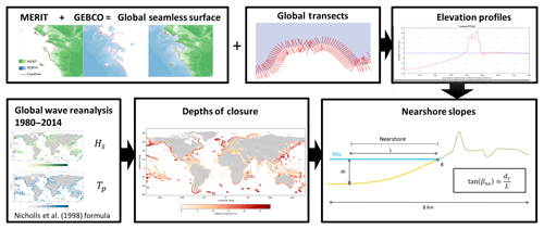
2.1 Workflow to obtain nearshore slopes

The estimation of nearshore slope required the following steps (Fig. 1). First, a seamless topo-bathymetric map was created (Sect. 2.2.1), and then cross-shore transects were drawn with an accompanying elevation profile (Sect. 2.2.2). Using global wave data the depths of closure were determined (Sect. 2.3), after which the nearshore slopes could be determined (Sect. 2.4).

Figure 1 Work flow followed for the calculation of the nearshore slopes worldwide.

2.2 Coastal profiles

2.2.1 Global topo-bathymetric data

A cross-shore contiguous representation of the coastal profile is needed in order to accurately derive geometrical parameters such as the nearshore slope. Presently, elevation data are separated between topographic, i.e., representing the subaerial surface of the Earth, and bathymetric, i.e., representing the subaqueous seabed. Here we merge two of these datasets in order to create a seamless elevation layer with a smooth transition between land and water.

The topographic layer that was used is the MERIT digital elevation model (DEM) (Yamazaki et al., 2017), which is an improved version of the existing spaceborne DEMs SRTM3 v2.1 (Farr et al., 2007) and AW3D-30m v1 (Tadono et al., 2015), after removing multiple error components (i.e., absolute bias, stripe noise, speckle noise, and tree height bias). It represents the terrain elevations at a 3 arcsec resolution (∼ 90 m at the Equator) and covers land areas between 90^∘ N and 60^∘ S, referenced to the EGM96 geoid. The bathymetric layer was obtained from the General Bathymetric Chart of the Oceans (https://www.gebco.net, last access: 15 September 2018), which is based on ship track soundings with interpolation between soundings guided by satellite-derived gravity data. The version used was the GEBCO_2014 Grid (Weatherall et al., 2015), which has a 30 arcsec resolution (∼ 900 m at the Equator) and it is generated by the aggregation of heterogeneous data types assuming all of them to be referred to MSL.

As the two datasets might overlap, the Open Street Map (OSM) (OpenStreetMap contributors, 2015) coastline was used to create a mask for land and water. For the final elevation dataset, a common grid was used, with a resolution corresponding to the higher resolution of the MERIT DEM dataset. Subsequently, the bathymetric data were interpolated only at the cells seaward of the OSM coastline. This was performed by a linear interpolation of the values at neighboring grid points in the x and y dimensions. One of the key elements when merging bathymetry and elevation data is to create a smooth transition between land and water. We have applied a low-pass filter to decrease disparities between pixel values by averaging nearby pixels. The smoothing technique was applied only on the cells along the coastline. For each cell the vertical offset Δz was computed (as the difference in elevation with respect to its neighboring cell). For the smoothing procedure different windows (i.e., number of grid cells around the grid cell to be smoothed) were used according to Δz. Smoothing window sizes of 3×3 were applied at areas where Δz was up to 10 m, 5×5 grid cells where Δz was higher than 10 m, and 9×9 in a few geographic areas where topography data present a big discrepancy with respect to the bathymetry.

2.2.2 Global elevation transects

The global coastline was defined using the OSM dataset of 2016. Since the full-scale coastline was found to be too detailed for the purposes of the present work, the level 8 generalized version of the dataset was used, which is a smoothed version that removes small details and has been previously used in global coastal assessments (Luijendijk et al., 2018). About 1 000 000 cross-shore transects were defined along the OSM coastline, spaced at 1 km intervals. To ensure a globally consistent spacing and length of the transects, the coastline was re-projected to the local UTM projection, before creating the transects. The middle point of each transect was defined at the OSM location, with a 4 km extension in both the landward and seaward directions. The profile length was chosen after testing different lengths to ensure that the active coastal profile is captured while minimizing data storage. The 1 km spacing was chosen in order to have a good coverage of the alongshore variability of the coastal profiles, while keeping the computational costs at a feasible level. Along each transect, a set of equidistant points was defined at an interval of 25 m, while flagging the locations where the elevation values were extracted from the global grid. For each transect the longitude and latitude of the extraction points were used to sample from the global merged elevation grid and create a continuous elevation profile.

The global transects (∼ 1 000 000) were first filtered to exclude transects located along coasts covered with ice, river inlets, or major ports, using the global transects of Luijendijk et al. (2018). This reduced the total number of transects to about 780 000 transects. Additionally, and specifically for the application described in Sect. 4.2, the sandy beach location data from Luijendijk et al. (2018) were used in order to identify the transects that were sandy, resulting in about 215 000 sandy transects. Note that gravel beaches are included in this dataset and are herein referred to as sandy.

2.3 Calculation of the depth of closure

The depth of closure was calculated using the formulation of Nicholls et al. (1998):

$$\begin{array}{}\text{(1)}& d_{\text{c}}=\mathrm{2.28}{H}_{\text{e},t}-\mathrm{68.5}\left({\displaystyle \frac{H_{\text{e},t}^{\mathrm{2}}}{g{T}_{\text{e},t}^{\mathrm{2}}}}\right),\end{array}$$

where H_e,t is the significant wave height that is exceeded only 12 h per t years, T_e,t is the associated wave period, and g is the gravitational acceleration. The selection of the length of the time series t in this formula is directly associated with the temporal scale of the application of the depth of closure. This means that, for example, applications that consider temporal scales on the order of decades (i.e., coastline models, Bruun rule) should use a t that is consistent with the assessment scale. Naturally, the temporal extent of the time series is dictated by the length of the available observations or modeling results. For example, Udo and Takeda (2017) applied Eq. (1) for SLR-induced coastal recession assessments along the Japanese coast taking into account the effects of timescale for their 100-year Bruun rule application by using the maximum wave heights in their 5-year-long wave record.

Here we applied Eq. (1) using the full time series of significant wave heights H_s and peak wave periods T_p from the global reanalysis covering the period between 1980 and 2014 presented by Vousdoukas et al. (2017). Waves were simulated using the third-generation spectral wave model WW3. The model has been extensively validated and detailed information can be found in the reference provided. The wave parameters were available every 3 h at offshore locations covering the ice-free coasts. Following Nicholls et al. (1998) here we calculate H_e,t as the wave height that is not exceeded more than 12 h over the full 34-year time series. This approach is expected to lead to larger d_c values than taking the yearly statistics, as larger waves will be included in the time series.

2.4 Estimation of the nearshore slope

For each of the transects, the cross-shore location of the depth of closure d_c was identified using the elevation profile and the d_c value derived as described in this section. The location of the depth of closure was calculated by finding the first (i.e., moving from the most offshore point towards land) point, which was shallower than the d_c and then linearly interpolating in between the adjacent cross-shore points along the transect. Then the cross-shore location of the shoreline (MSL) point was estimated using a similar method. In case of multiple shoreline points (e.g., barrier islands) the point that was located closer to the OSM defined point was chosen. The cross-shore distance between these two points was used as the horizontal length of the nearshore area L. The nearshore slope tan (β_ns) was then calculated as the ratio $\frac{d_{\text{c}}}{L}$ .

At locations in which the calculation could not be carried out as described above, an error code was assigned to describe the cause of the calculation failure (Figs. S1–S2 in the Supplement). For example, as the OSM coastline does not represent the open coast only, but includes a substantial number of areas with elevation that is far from the conventional profile presented in Fig. 1, the calculation of the slope in this way was not always successful. This was typically the case for coastlines dominated by fjord features (e.g., Norway, Chile). Furthermore, some transects did not have any offshore point in close proximity for the calculation of the depth of closure. The transects of which the nearshore slope could not be calculated were about 160 000 of the total 780 000. Almost 20 % out of these 160 000 transects were identified as sandy.

At some other locations (mostly embayed or protected areas) the depth of closure point was located seaward of the most offshore profile point. Therefore, the deepest point was taken as the depth of closure d_c. Additionally, due to the merging process of the bathymetric and topographic elevation data, elevation steps close to the shoreline were observed in some transects. These transects were determined by identifying abrupt changes of the slope close to the shoreline. A warning code was also assigned to such transects (Figs. S1–S2).

3 Results

3.1 Global depths of closure

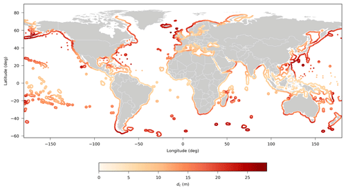
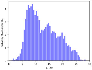
The resulting global distribution of d_c (Fig. 2) showed that on open-ocean coasts, d_c generally increased with latitude because of the wave height, while d_c was smaller along the shores of more wave-sheltered seas. The global average value of d_c was approximately 13 m, while it reached values of more than 20 m at some areas at higher latitudes (Fig. 3).

Figure 2 Depths of closure d_c along the global coastline using the formulation by Nicholls et al. (1998) (Eq. 1).

Figure 3 Histogram of the probability of occurrence of d_c globally (using bins of 0.5 m).

3.2 Nearshore slopes

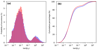
The calculated nearshore slopes (Athanasiou, 2019) showed high spatial variability globally (Fig. 4 with continental zooms in Figs. S3–S8). The histogram of the calculated nearshore slopes (Fig. 5a) revealed that the most commonly computed nearshore slopes were around 0.005. Additionally, there was a high probability of occurrence of nearshore slopes larger than 0.2 due to the high number of transects at fjords and other steep coastlines. Furthermore, we detected several mildly sloping locations (i.e., nearshore slope lower than 0.002). Such mildly sloping coastlines are mostly characterized by high tidal range and/or muddy coastlines (e.g, northwest Australia). The median nearshore slope worldwide was 0.007, while the 10th and 90th percentiles were 0.001 and 0.565, respectively (Fig. 5b). When only the sandy transects were considered (see Sect. 2.2.2), the most common nearshore slope shifted to 0.01, which corresponds with the globally uniform profile slope assumed in previous global-scale studies (Hinkel et al., 2013).

The nearshore slope value is dependent on various geological and hydrodynamic factors, such as wave characteristics, sediment size, sediment supply, and large-scale geological and tectonic processes, among others. For that reason we aggregated the nearshore slopes along various regions around the world, defined heuristically considering geographical proximity and their corresponding oceans or seas. A distinct variation in the nearshore slopes can be seen among regions (Fig. 6). The three regions with the on average steeper slopes were the Pacific Islands, the Norwegian Sea, and the Mediterranean Sea with median values of 0.025, 0.020, and 0.014, respectively. On the other hand, the three regions with the mildest nearshore slopes were northern Australia, the eastern US, and the Gulf of Mexico and Southeast Asia with median values of 0.001, 0.002, and 0.003, respectively. The variance of the aggregated nearshore slopes per region (defined as the logarithmic difference between the 5th and 95th percentile) varied, with western South America and northern Australia showing the highest and lowest variance, respectively.

4 Comparison with local observations

4.1 Depth of closure

Different methods exist to estimate the d_c and therefore the validation of this parameter can be quite challenging at a global scale. A thorough validation of the estimated depths of closure would demand various local bathymetrical surveys with good spatial resolution and sufficiently long temporal resolution and extent (i.e., 34 years of data). This kind of information is not readily available. Therefore, here we compare our results with a study at the US coast (Brutsché et al., 2016), which employed various formulas to calculate d_c, including Eq. (1). We compared the d_c at the offshore locations of the US coast (Fig. 2) with the d_c of the closest point from Brutsché et al. (2016), calculated using the same formula (Eq. 1). Our predicted d_c showed skill in capturing the spatial variation as calculated by Brutsché et al. (2016) (Fig. S9), but presented a positive bias of 3.34 m (Fig. S10). This can be attributed to the different location and temporal scale of the wave statistics (i.e., Brutsché et al. (2016) used nearshore transformed wave time series of a 20-year hindcast).

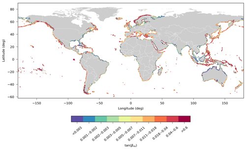
Figure 4 Global map of nearshore slopes. Red colors indicate steeper slopes while blue colors indicate milder slopes. Note that in the color scale the slopes have been grouped in non-equidistant increments in order to highlight the spatial differences.

Figure 5 (a) Histogram of the probability of occurrence of nearshore slopes. (b) Cumulative probability distribution of nearshore slopes. The graphs have been plotted for all transects (blue) and only for sandy transects (red). Note that the x axis is plotted on a log scale.

4.2 Nearshore slopes

The computed slopes were validated both qualitatively and quantitatively. The former was performed regionally using coastal classifications of the European and the Mediterranean coastlines, while the latter employed observations at sandy beaches derived from local surveys at eight study sites around the world.

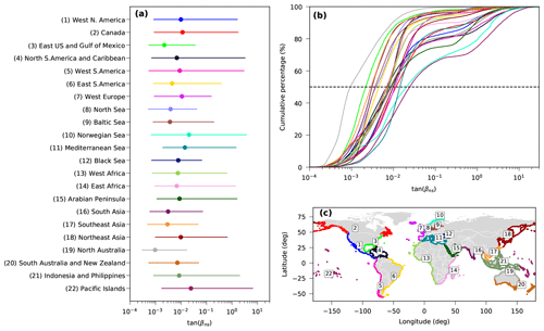
Figure 6 (a) Nearshore slope statistics per region. Dots indicate the median, while lines indicate the range between the 5th and 95th percentiles. (b) Cumulative probability distribution of nearshore slopes per region. Dashed line indicates the 50 % line. (c) Global map with the defined regions with their respective color and ID. Note that (a) and (b) use the color scheme indicated by (c). The x axis of (a) and (b) are plotted at a log scale.

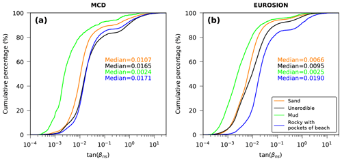
Figure 7 Cumulative probability distribution of nearshore slopes per coastal type for the (a) MCD dataset and (b) EUROSION dataset. The median values per coastal types are plotted with their respective colors as indicated in the legend. Note that the x axis is plotted on a log scale.

4.2.1 Qualitative validation

Two coastal classification datasets were used to inspect the computed nearshore slopes grouped according to geomorphological coastal types. One was the Mediterranean coastal database (MCD) (Wolff et al., 2018), which classifies the Mediterranean coastline in four classes: (1) sandy beaches, (2) unerodible coasts, (3) muddy coastlines, and (4) rocky coasts with pocket beaches. The other was the EUROSION geomorphological classification (EUROSION, 2004) of the countries of the European Union (EU), which includes 20 different coastal types. The latter was reclassified to the four classes of the MCD database in order to reduce the total number of classes (Fig. S11)

The calculated nearshore slopes followed the expected variability between the different coastal typologies for both classification datasets (Fig. 7). For example, muddy coastlines had relatively milder nearshore slopes (median values of 0.0024 and 0.0025 for MCD and EUROSION datasets, respectively). Sandy coastlines had a median nearshore slope of 0.0107 and 0.0066, respectively, for the MCD and EUROSION datasets, which relates to the steeper sandy beach slopes observed along the Mediterranean coastline. Unerodible and rocky coastlines had on average relatively steeper slopes.

Table 1 Validation case study descriptions.

Figure 8 Field sites used for validation of the estimated global nearshore slopes.

4.2.2 Quantitative validation

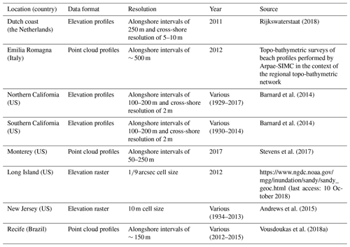
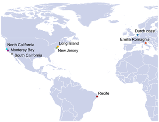
The study sites for the quantitative validation were selected according to data availability and a criterion of having at least 20 transects overlapping with the derived global dataset to enable the computation of error statistics per site. The validation focused only on sandy coastline transects that are not adjacent to morphologically complex areas (e.g., inlets, river mouths) determined using satellite imagery. The ground truth sites (Fig. 8; Table 1) represent different coastal geomorphologies with varying hydrodynamic forcing and span across different continents. We performed the validation on the basis of the nearshore slopes, using the d_c values that were derived from the global analysis of wave data described in Sect. 2.2.2, for both local and global nearshore slope estimation. The local nearshore slope was calculated using the methodology described in Sect. 2.3.

Table 2 Error statistics per validation site on the basis of the nearshore slopes tan (β_ns).

When the elevation was represented by locally defined profiles, the comparison was performed using the closest globally derived transect. When point cloud data were available, they were first interpolated on a common grid and then the elevation was extracted along the global transects. The same process was performed when an elevation raster was available.

For a quantitative evaluation of the accuracy of the globally predicted slope values against the locally observed ones, various statistical parameters were calculated per site, as well as globally. This included the coefficient of determination R², the normalized mean bias (NMB) and the normalized root-mean-square error (NRMSE). Note that there is no temporal coherence between the predicted and observed data since the global elevation dataset is a merged product from temporally varying bathymetric sources (see Sect. 2.2.1) and the observed data were taken at different times. Therefore, it is expected that part of the calculated errors are due to potential temporal differences of the estimated and observed elevation data.

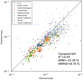
Figure 9 Linear regression between globally predicted nearshore slopes and nearshore slopes observed from local data for all study sites. Note that both axes are on a log scale.

A regression analysis performed over all of the available global observations resulted in a normalized mean bias of almost −25 % and an R² value of 0.44 (Fig. 9), implying that extracted nearshore slopes captured the spatial variability of the ground truth data. The negative overall bias indicated that the calculated global slopes were on average milder than those observed.

The error statistics per validation site (Table 2) showed that overall, R² values were above 0.6 except for northern California, Recife, and southern California where poorer agreement was found (i.e., 0.38, 0.25, and 0.3, respectively). At all validation sites (except Monterey Bay) a negative bias was observed. The NRMSE varied per study site, with values lower than 35 % for five out of the eight validation sites. The high NRMSE at Emilia Romagna can be attributed to the quite high bias, but nevertheless the spatial variability was captured correctly (R²=0.7). It should be noted that the number of overlapping sandy transects differed significantly between sites as the spatial extent of the available local surveys differed. For example, at Emilia Romagna and Monterey Bay there were only 25 and 27 overlapping transects, while at southern California there were 382.

5 Discussion

5.1 Spatial variation in nearshore slopes

As discussed in the previous section the results of the present study revealed a quite pronounced spatial variation in nearshore slopes worldwide (Fig. 4). For example, the west coast of North and South America had on average steeper slopes in comparison to the east, which can be attributed to the swell-dominated wave climate along the former (the same holds for the west and east coasts of Africa). The classification of the coasts with respect to the plate tectonics (Inman and Nordstrom, 1971) seems to be relevant to nearshore slope distribution as well. Trailing edge coast with wider continental shelf width (e.g., North Sea, east coast of North and South America, North Australia) appeared to have milder nearshore slopes than leading edge coasts (e.g., west coast of North and South America and the biggest part of the Mediterranean). Sediment grain size can play an important role as well in the shape and slope of the nearshore profile (Dean, 1991). The coasts of the Gulf of Mexico and South and Southeast Asia showed on average mild nearshore slopes, which can be attributed to the large (historic) sediment supplies by some major rivers therein. The local slope values are ultimately the results of the combination of all the physical processes mentioned previously. At sedimentary coasts the upper nearshore profile is mainly influenced by waves while the lower one is influenced by tectonics, sediment supply, or major storm events.

5.2 Improvements in estimations of SLR-induced retreat of sandy coasts

Similarly to the overall dataset (including non-sandy coasts), the subset of nearshore slopes of sandy coasts displays a considerable spatial variation, even though the commonly used 1 : 100 nearshore slope assumption (Hinkel et al., 2013) lies in the most probable range (Fig. 5). Using the Bruun rule (Bruun, 1962), we investigated the effect of applying the spatial variation in the nearshore slope on the estimation of shoreline retreat due to sea level rise, in comparison with applying a uniform 1 : 100 slope as commonly done for sandy beaches.

The Bruun rule is a simple two-dimensional mass conservation principle, which predicts a landward and upward response of sandy profiles as a response to SLR. It is expressed as (Bruun, 1962)

$$\begin{array}{}\text{(2)}& R={\displaystyle \frac{L}{d_{\mathrm{c}}}}S,\end{array}$$

where R is the horizontal coastal recession, d_c is the depth of closure, L is the horizontal length from the shoreline to the depth of closure, and S is the SLR. While used extensively for lack of a more efficient method, its use has been a controversial matter in literature during the last years (Cooper and Pilkey, 2004; Ranasinghe and Stive, 2009), as it is based on a number of assumptions and simplifications (i.e., equilibrium profile existence, cross-shore sediment balance). Nevertheless it is the only method that can deal with coastal recession due to SLR at a large scale in a computationally feasible manner. Since $\tan \left({\mathit{\beta }}_{\text{ns}}\right)=\frac{d_{\text{c}}}{L}$ this makes Eq. (2)

$$\begin{array}{}\text{(3)}& R={\displaystyle \frac{\mathrm{1}}{\tan \left({\mathit{\beta }}_{\text{ns}}\right)}}S.\end{array}$$

Physically, there are limits of the nearshore slopes that can be encountered at sandy beaches related to the angle of repose of granular materials. For our dataset, the sandy transects (Luijendijk et al., 2018) were found to lie beyond these ranges in some cases. This can be attributed to local effects of geology and sediment budget but also to data and methodological artefacts. Therefore, we applied upper and lower limits of 0.2 and 0.001 for the sandy nearshore slopes and constrained the slopes that lie beyond these limits to the limit values.

Following the linear relationship between the coastal recession R and the nearshore slope in Eq. (3), the differences in the coastal recession under a given SLR scenario can show significant spatial variations. In order to highlight this, the ratio between the coastal recession R_calc (i.e., using the nearshore slopes presented herein) and R₁₀₀ (i.e., using a 1∕100 nearshore slope globally) was estimated globally for all sandy transects (Fig. 10). The results indicate that for a large number of areas around the world the assumption of 1 : 100 nearshore slopes underestimates the potential coastal recession with a median $\frac{R_{\mathrm{calc}}}{R_{\mathrm{100}}}$ of 1.39. However, it should be noted that there are also several locations with steeper slopes, where the 1 : 100 assumption overestimates the SLR-induced erosion.

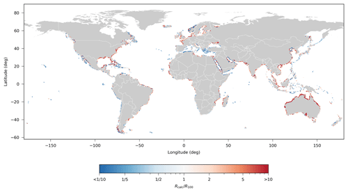
Figure 10 Global map of $\frac{R_{\mathrm{calc}}}{R_{\mathrm{100}}}$ where red colors indicate locations where the $\tan \left({\mathit{\beta }}_{\text{sf}}\right)=\mathrm{1}:\mathrm{100}$ assumption underestimates the coastal recession while blue colors indicate locations where it overestimates it. Note that the color bar uses a log scale.

In order to highlight the potential impact of this effect, a coastal recession estimate was computed for all transects of each region (see Fig. 6) using Eq. (3) for an arbitrary SLR of 0.5 m across the global coastline. The median value of the coastal recession of all transects per region was calculated as a robust description of its central tendency (Fig. 11) and compared with the value of 50 m (which is the recession that would be calculated for a SLR of 0.5 m using the 1 : 100 slope assumption). The results show that, in most of the defined regions the assumption of a 1 : 100 nearshore slope would result in the underestimation of coastal recession, especially in northern Australia, South and Southeast Asia, and the eastern US and Gulf of Mexico regions. However in some of the regions, such as the Mediterranean and Norwegian seas and the west coast of North and South America, the 1:100 slope assumption would lead to an overestimation due to the steeper nearshore slopes encountered on average there.

5.3 Limitations

The global scale of the present work introduced inevitable limitations related to data availability, computational efficiency, and methodological constraints. Merging bathymetric and topographic data at a global scale can be quite challenging. This is associated with differences in spatial resolution and potential overlaps or differences in the vertical datum. Here we tried to resolve these issues by using the OSM coastline as the MSL to differentiate between sea and land and connect the elevation data. Although other available coastline datasets exist, either they have a coarser resolution, therefore not allowing for a correct representation of the separation between land and water, or they do not have a global coverage. The importance of the coastline and DEM data has been previously highlighted with respect to statistics of exposure information (Lichter et al., 2011). We expect that the choice of the coastline can have an effect in the elevation profiles, especially in areas with a high tidal range.

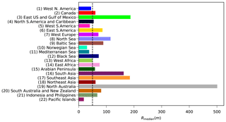
Figure 11 Median coastal recession in meters, calculated per region for the sandy transects assuming 0.5 m of SLR across the global coastline. The vertical dashed line indicates the recession of 50 m, which would be the result if a 1∕100 nearshore slope was assumed.

Additionally, GEBCO is a combination of bathymetric data derived from variable sources and different techniques and in some cases might have differences in the vertical datum (Weatherall et al., 2015). This might introduce regional differences in the trustworthiness of the results. The smoothing procedure that was applied to the bathymetric and topographic data may have affected the nearshore slope values, especially at cliffed coastlines, where the computed slopes may be milder than the reality. Nevertheless, cliffed transects retained quite steep values as can be seen by the second peak in the global slope distribution (Fig. 5). Furthermore, we expect that at locations where the nearshore slopes are steep, the resolution of the bathymetry is not high enough to capture a large number of bathymetry points between the shoreline and the depth of closure, hiding the details of the profile. We believe that when bathymetrical datasets with better resolution and accuracy become available in the future, the presented technique can be applied to update the global nearshore slope estimations.

The wave statistics that were used to determine the depth of closure across the global transects of the present study were taken from the closest offshore point of the wave reanalysis output (see Sect. 2.3). Ideally, the wave time series of the 28 years used here should be transformed to nearshore conditions at a location just offshore of the depth of closure using Snell's law. This would require an assumption of a nearshore slope, then the calculation of d_c, and then the recalculation of the nearshore slope using an iterative approach until the slopes converge. This was deemed to be outside the scope of this study, considering the large number of transects. Nevertheless, we found that the nearshore slopes were not very sensitive to small changes in the depth of closure.

With respect to the comparison of the dataset compiled in the present study with available observations (Sect. 4), it should be mentioned that due to the scale of the study, it is quite challenging to perform a direct validation with the same spatiotemporal conditions. For example the comparison of the estimated d_c was performed against the results of a study that used the same formula, but employing wave statistics with different temporal extent and at different locations (Sect. 4.1). Additionally, the local surveys used for the quantitative comparison of the nearshore slopes had various sources, used different measuring techniques, and were collected at different times (Sect. 4.2.2). Naturally, it is expected that these spatiotemporal differences had an impact on the error statistics computed herein. More long-term coastal profile datasets, including coastal sites in diverse coastal environments, are needed to ensure a thorough validation of our dataset. The wealth of long-term satellite data combined with the constantly evolving remote sensing techniques can potentially be an avenue to consider in the future.

In this study the nearshore slope was defined from the depth of closure until the shoreline. This could be a deviation from certain Bruun rule implementations that define the active profile slope from the depth of closure until the dune or berm crest (Zhang et al., 2004; Hinkel et al., 2013; Toimil et al., 2017; Udo and Takeda, 2017). Given that the available global topographic datasets lack the resolution to resolve dunes or berms (Vousdoukas et al., 2018b), their inclusion in the analysis was not feasible, potentially resulting in an underestimation of the active profile slope (from the depth of closure to the top of the dune) along beaches with prominent dune systems. Nevertheless, since our dataset includes the nearshore slope and the depth of closure, one could calculate the slope from depth of closure to the dune or berm height if this information is available locally.

Another important matter is the sensitivity of the estimated nearshore slopes to the depth of closure values used in this study. In order to test the robustness of our dataset, and how different wave statistics or depth of closure formulae could affect our estimations, we varied the previously calculated d_c values (Sect. 2.3). Changes of −20 %, −10 %, 10 %, and 20 % of the originally estimated d_c were tested. The normalized differences of the estimated nearshore slopes had moderate sensitivity to the depth of closure variation (Fig. S12). When the depth of closure was increased and decreased by 10 %, at almost 70 % of the transects, the nearshore slope changed by the same percentage. On the other hand, with an increase and decrease in the d_c by 20 %, the nearshore slope difference was on the order of 20 % at about 75 % of the transects. The number of transects with changes up to 20 % was higher when only the sandy transects were considered. In general, the largest increase in the nearshore slope was observed when d_c was decreased. The spatial distribution of the relative nearshore slope changes showed that in most cases the sensitivity was low. The most sensitive areas to changes in d_c were areas with steep slopes (e.g., fjord areas in Norway, Chile, and others) (Fig. S13).

6 Data availability

The final output data provide the location of each of the ∼ 780 000 points along the global coastline together with (a) the depth of closure d_c, (b) the nearshore slope tan (β_ns) and (c) an error/warning code in case the slope was not calculated or limitations in the profile were spotted. These data are given as a comma-separated value file. The data can be downloaded via https://doi.org/10.4121/uuid:a8297dcd-c34e-4e6d-bf66-9fb8913d983d (Athanasiou, 2019).

7 Conclusions

A dataset of the global distribution of nearshore slopes at an alongshore resolution of 1 km is presented, using global elevation datasets and wave statistics. Depths of closure d_c were estimated worldwide using an empirical formulation and long-term wave statistics derived from 34-year wave reanalysis. The average d_c globally was almost 13 m, attaining larger values at higher latitudes. The global median nearshore slope was 0.007, while most values were in the range 0.001 to 0.565 (10th and 90th percentiles, respectively). The most commonly computed nearshore slope was about 0.005, which increased to 0.01 when only sandy coasts were considered. However, the computed nearshore slopes exhibited substantial spatial variability, potentially corresponding with spatial variations in hydrodynamic forcing and geological conditions. The dataset captured expected qualitative nearshore slope patterns when compared to available coastal classification datasets. Additionally, it captured the spatial variability of the nearshore slopes of sandy beaches at eight validation sites from around the world, but with a negative bias of 25 % (milder slopes than the observed ones).

The assessment of SLR-driven coastline recession (for an arbitrary 0.5 m SLR) with globally uniform coastal slopes, as performed in many previous studies, and the spatially variable nearshore slopes computed herein showed large differences between the recession amounts projected by the two approaches. Worldwide, the median coastline recession calculated with the nearshore slopes computed here was almost 40 % larger than that computed by assuming a globally uniform 1 : 100 coastal slope, with the ratio between the two estimates varying substantially around the world. We believe that this dataset is a first step towards capturing the spatial variability of coastal profile characteristics and enabling a correct spatial representation of coastal impacts.