the Creative Commons Attribution 4.0 License.
the Creative Commons Attribution 4.0 License.
 | 02 Aug 2019
GRACE-REC: a reconstruction of climate-driven water storage changes over the last century
Vincent Humphrey
Lukas Gudmundsson
The amount of water stored on continents is an important constraint for water mass and energy exchanges in the Earth system and exhibits large inter-annual variability at both local and continental scales. From 2002 to 2017, the satellites of the Gravity Recovery and Climate Experiment (GRACE) mission have observed changes in terrestrial water storage (TWS) with an unprecedented level of accuracy. In this paper, we use a statistical model trained with GRACE observations to reconstruct past climate-driven changes in TWS from historical and near-real-time meteorological datasets at daily and monthly scales. Unlike most hydrological models which represent water reservoirs individually (e.g., snow, soil moisture) and usually provide a single model run, the presented approach directly reconstructs total TWS changes and includes hundreds of ensemble members which can be used to quantify predictive uncertainty. We compare these data-driven TWS estimates with other independent evaluation datasets such as the sea level budget, large-scale water balance from atmospheric reanalysis, and in situ streamflow measurements. We find that the presented approach performs overall as well or better than a set of state-of-the-art global hydrological models (Water Resources Reanalysis version 2). We provide reconstructed TWS anomalies at a spatial resolution of 0.5∘, at both daily and monthly scales over the period 1901 to present, based on two different GRACE products and three different meteorological forcing datasets, resulting in six reconstructed TWS datasets of 100 ensemble members each. Possible user groups and applications include hydrological modeling and model benchmarking, sea level budget studies, assessments of long-term changes in the frequency of droughts, the analysis of climate signals in geodetic time series, and the interpretation of the data gap between the GRACE and GRACE Follow-On missions. The presented dataset is published at https://doi.org/10.6084/m9.figshare.7670849 (Humphrey and Gudmundsson, 2019) and updates will be published regularly.
- Article
(9856 KB) - Full-text XML
-
Supplement
(1347 KB) - BibTeX
- EndNote


Because the amount of freshwater available on land controls the development of natural ecosystems as much as human activities, terrestrial water storage (TWS) represents a critical variable of the Earth system. Changes in TWS can be caused by both anthropogenic and natural processes. Natural variability in ocean and atmospheric circulation, such as the El Niño–Southern Oscillation (ENSO), is responsible for anomalies in precipitation which strongly influence water storage (Ni et al., 2017), leading to regional droughts and floods with large impacts on human activities (Veldkamp et al., 2015). At the global scale, climate-driven fluctuations in the total amount of water stored on land have been linked to a wide range of geophysical phenomena, including changes in global mean sea level (Cazenave et al., 2014; Reager et al., 2016; Rietbroek et al., 2016; Dieng et al., 2017), changes in global carbon uptake by land ecosystems (Humphrey et al., 2018), and the motion of the Earth's rotational axis (Adhikari and Ivins, 2016; Youm et al., 2017). In addition to climate-driven natural variability, human activities also influence terrestrial water storage, for instance through groundwater depletion (Rodell et al., 2009; Chen et al., 2016), building of dams (Chao et al., 2008), or the impact of anthropogenic climate change on land ice (Jacob et al., 2012).
From 2002 to 2017, changes in terrestrial water storage (TWS) have been measured by the GRACE satellites with an unprecedented accuracy. Because these observations integrate both natural and anthropogenic effects across all water reservoirs (i.e., soil moisture, groundwater, snow, lakes, wetlands, rivers, and land ice), isolating the contribution of specific reservoirs or the relative importance of natural versus anthropogenic effects is still relatively uncertain and has been the focus of several recent publications (Reager et al., 2016; Eicker et al., 2016; Wada et al., 2016; Fasullo et al., 2016; Felfelani et al., 2017; Getirana et al., 2017; Pan et al., 2017; Andrew et al., 2017; Rodell et al., 2018; Hanasaki et al., 2018; Khaki et al., 2018; WCRP Global Sea Level Budget Group, 2018). In this context, one critical aspect is to model the effect of climate variability on TWS changes. At this time, only global hydrological models and land surface models can provide long-term estimates of natural TWS variability; however, they are usually not calibrated against GRACE measurements and sometimes exhibit large biases in TWS amplitude (Schellekens et al., 2017; Zhang et al., 2017; Scanlon et al., 2018). Typically, only a small number of such model runs is available and exploring the uncertainty related to the use of different meteorological forcing datasets is not possible. With this paper, we aim to address these shortcomings with a computationally cheap alternative. Unlike hydrological models which represent physical processes and model water reservoirs individually (e.g., snow, soil moisture, lakes), we train a statistical model to directly reconstruct the total TWS changes from precipitation and temperature information.
The primary objective of this paper is to provide long and consistent time series of climate-driven TWS variability. Although the temporal coverage of GRACE observations will be extended by the GRACE Follow-On mission launched on 22 May 2018, there will be a temporal gap of approximately 1 year between the two missions. The reconstruction provided here is calibrated against GRACE measurements and can be used to interpret this data gap and reconcile the two datasets. In addition, we provide a century-long TWS reconstruction that can be used to study past natural TWS variability. We expect that this product will be relevant to sea level budget studies (Chambers et al., 2016; Cheng et al., 2017; Frederikse et al., 2018; WCRP Global Sea Level Budget Group, 2018), the analysis of climate signals in geodetic time series (in GRACE or in ground GNSS measurements, for example), development of daily hydrological loading models (Dill and Dobslaw, 2013; Moreira et al., 2016), and global to regional assessments of the recurrence of extreme hydrological droughts and their impact on ecosystems (Sheffield and Wood, 2007; Sheffield et al., 2012; Beguería et al., 2014; Griffin and Anchukaitis, 2014; Kusche et al., 2016; Dai and Zhao, 2016; Spinoni et al., 2017; Heim, 2017; Rudd et al., 2017; Sinha et al., 2017; Haslinger and Blöschl, 2017; Um et al., 2017; Bento et al., 2018; D'Orangeville et al., 2018; Huang et al., 2018; Markonis et al., 2018; Anderegg et al., 2018; Gao et al., 2018).
2.1 GRACE products
The two different monthly GRACE solutions used here (Table 1) are obtained using the so-called mass concentration (mascon) technique. This technique provides estimates of mass changes over small predefined regions, which are referred to as mascons. The two solutions differ in terms of the employed processing algorithms and also in terms of the models used to correct for the effect of glacial isostatic adjustment (GIA). For more general information on the GRACE mission, gravity recovery techniques and processing, we refer the reader to the reviews of Wouters et al. (2014) or Wahr (2015).

2.2 Precipitation and temperature
We use three different precipitation products which are aimed to address the needs of various user communities (Table 2). The multisource weighted-ensemble precipitation dataset (MSWEP) merges a large number of existing precipitation products, including satellite-based, rain-gauge-based and reanalysis products (Beck et al., 2017, 2018). We expect this dataset to provide a best estimate for the period 1979–2016. The Global Soil Wetness Project Phase 3 (GSWP3) forcing dataset (Kim, 2017) is based on the 20th Century Reanalysis (20CR) version 2c (Compo et al., 2011). The original 20CR precipitation fields produced at a resolution of 2∘ are dynamically downscaled using spectral nudging and bias-corrected using observations from the Global Precipitation Climatology Project (GPCP) and the Climatic Research Unit (CRU). With this dataset, we aim to provide a homogeneous long-term reconstruction of climate-driven TWS changes over the period 1901–2014. Third, we use precipitation estimates from the European Centre for Medium-Range Weather Forecasts (ECMWF) re-analysis (ERA5), which cover the period 1979–present. With this dataset, we aim to provide frequent updates of reconstructed TWS anomalies which can, for instance, be used to investigate the data gap between the GRACE mission (decommissioned in October 2017) and the GRACE Follow-On mission launched in May 2018. For temperature, we use ERA5 air temperature in combination with MSWEP and ERA5 precipitation, and GSWP3 air temperature in combination with GSWP3 precipitation. We note that sensitivity analyses have shown that the choice of the temperature dataset has very little influence on the final product (not shown).

2.3 Modeling approach
2.3.1 Model formulation
A simple statistical model is calibrated at each GRACE mascon individually, meaning that model parameters are space-dependent. One model is calibrated for each combination of the two GRACE products (Table 1) with the three precipitation products (Table 2). The meteorological forcing is always spatially averaged over the spatial footprint of the GRACE mascons. Because the model described here does not have any explicit constraint in terms of mass or energy conservation, we refer to it as a statistical model; however its formulation is largely inspired from basic principles of hydrological modeling. Assuming a linear water store model, water outputs are directly proportional to the storage and to the residence time of the water store (e.g., Beven, 2012), so that the temporal evolution of the storage can be approximated as
where t is a daily time vector, TWS(t) is the storage, P(t) is the precipitation input, and τ(t) is the residence time of the water store.
Small (large) values of the residence time indicate that water inputs tend to leave the reservoir quickly (slowly), through either runoff or evapotranspiration. Here we introduce seasonal changes in residence time (e.g., related to snow accumulation during the cold season or increased evaporative demand during the warm season) using a temperature-dependent relationship. The residence time used in Eq. (1) is formulated as a function of de-trended daily air temperature:
where a and b are calibrated model parameters with a positive sign and TZ(t) is a transformation of the original de-trended daily air temperature T(t). The purpose of this transformation is to first make τ only sensitive to changes in temperature when temperature is higher than 0 ∘C,
and to moderate the influence of extreme temperature values by applying a sigmoid transform to the standardized temperature:
As a result of this transformation, TZ approaches a value of 1 (0) when temperature gets colder (warmer) and thus the residence time increases (decreases) (Eq. 2). Note that different or more complex formulations (e.g., also involving net radiation) were tested but did not yield significant improvement compared to the relatively simple approach presented here. The result of this model is illustrated in Fig. 1a, which depicts the temperature-dependent residence time (red line), the daily precipitation input (blue bars) and the resulting terrestrial water storage time series (blue line).
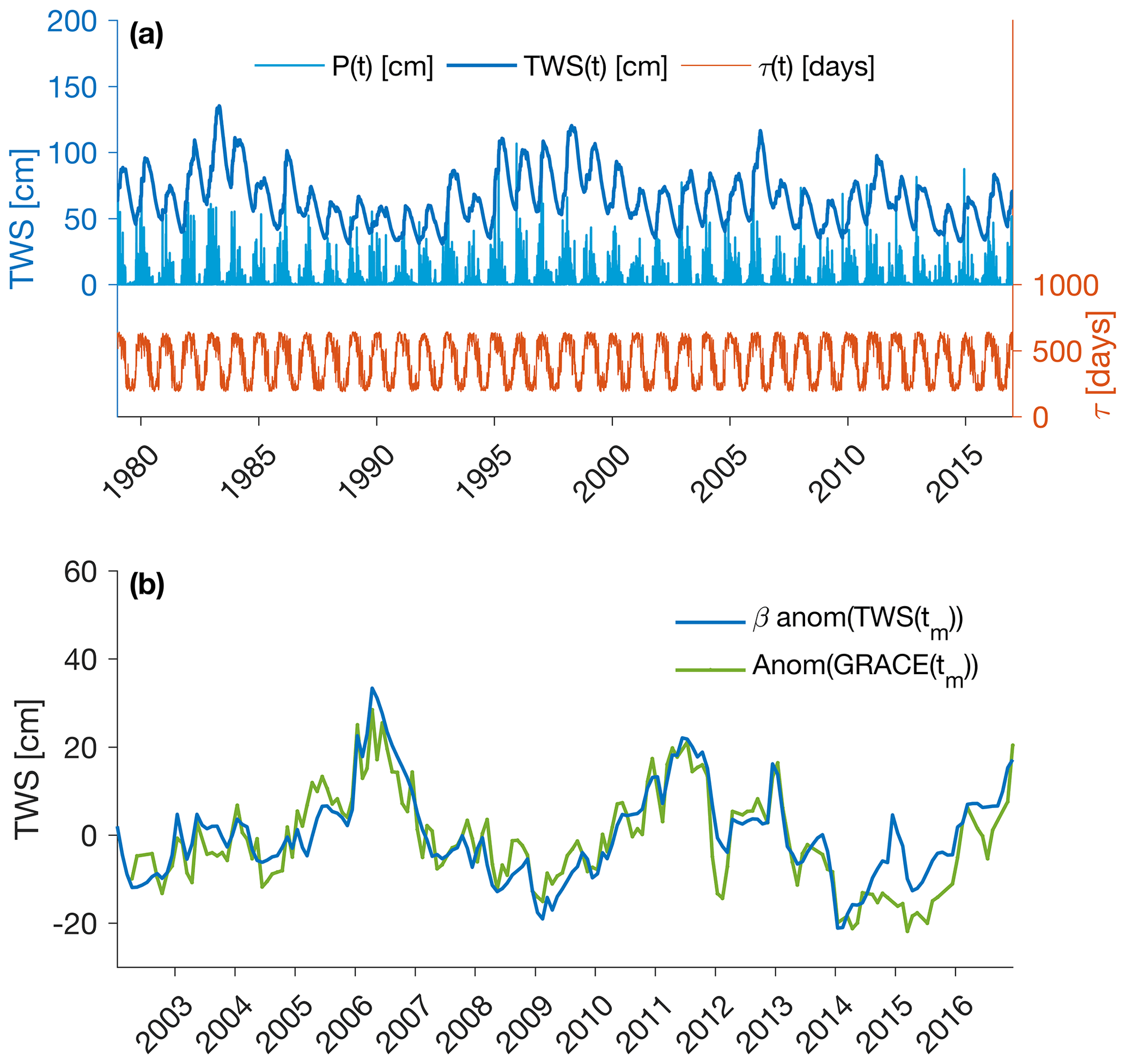
Figure 1Illustration of the GRACE reconstruction at one given mascon (located in California). (a) Input daily precipitation time series P(t), temperature-dependent residence time τ(t), and the resulting daily TWS time series TWS(t). (b) Agreement between GRACE and GRACE-REC after subtracting the seasonal cycle and long-term trend (zoomed over the period 2002–2017).
The initial value of the storage (TWS(t) at t=0) is computed from the analytical solution for the equilibrium state of Eq. (1) given the mean precipitation input and the mean residence time:
The initial value of the storage is thus obtained as the ratio between the mean rate of water input and the mean rate of water loss (also see the full development in the Supplement). Using this solution (Eq. 5) requires the assumption that the storage is close to equilibrium at the start of the reconstruction but avoids the loss of 6 years for model spin-up as was done in previous work (Humphrey et al., 2017). Still, we note that reconstructed TWS anomalies at the very beginning of the time series (typically the first year) should be interpreted with care.
2.3.2 Model calibration
The daily water storage time series (Eq. 1) is averaged to monthly temporal resolution (tm) in order to make it comparable with the monthly GRACE time series. Calibration is conducted at a monthly scale against de-seasonalized and de-trended GRACE TWS observations (Fig. 1b), such that
where β is a calibrated scaling factor, ε corresponds to an error term, and anom() is an operator indicating that the seasonal cycle and the linear trend are removed as mentioned above. The trends are removed during model calibration because many trends in GRACE are caused by anthropogenic activities (Humphrey, 2017; Rodell et al., 2018), which our climate-driven model cannot explain by definition. We note that as a result, the choice of the GIA model used in GRACE processing (Table 1) does not impact the model calibration. Removing the seasonal cycle lets the model focus on capturing the inter-annual variability correctly. The three model parameters (a, b: Eq. 2 and β: Eq. 6) are calibrated at each mascon using a Markov chain Monte Carlo (MCMC) procedure minimizing the sum of squares of the residuals between the predicted and observed monthly TWS anomalies (Haario et al., 2006; Humphrey et al., 2017). The MCMC procedure provides distributions of equally acceptable parameter sets which are later used in the generation of ensemble members (Sect. 2.4).
2.4 Generation of ensemble members at monthly resolution
2.4.1 Rationale for the generation of model ensembles
The empirical residuals (ε) in Eq. (6) correspond to the difference between observed and predicted water storage anomalies. They include measurement and leakage errors from GRACE, structural model errors, and errors introduced by the imperfect meteorological forcing. In this section, we aim to quantify and communicate the magnitude of these errors to end users in a practical way. A classical approach is to provide the standard error σε for every mascon (Fig. 2a):
Because it can be shown in our case that the residuals are normally distributed (Fig. 2b), it is relatively safe to use the standard error to estimate the predictive uncertainty (and any confidence interval) over a given mascon. However, in many applications, predictions from individual mascons need to be aggregated, for instance to compute basin-scale averages or global means. In this case, obtaining an error estimate for the aggregated value is not trivial because the spatial covariance of the errors needs to be taken into account during the error propagation (Bevington and Robinson, 2003). Because errors are spatially and temporally correlated, any averaging operation (in the time or space domain) potentially requires that error covariance is taken into account.
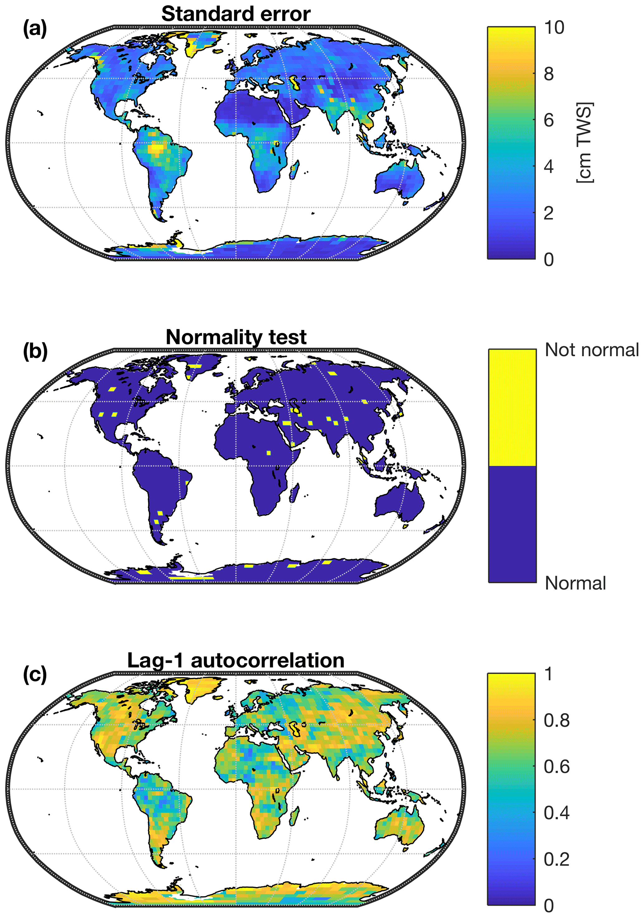
Figure 2Characterization of the empirical model residuals for the GRACE-REC dataset based on MSWEP precipitation and ERA5 air temperature, calibrated with the JPL mascons. (a) Standard model error. (b) Result of a Kolmogorov–Smirnov test for normality on the model errors (p<0.05); (c) lag-1 serial autocorrelation of the model errors.
To provide a practical solution to this problem, we generate ensemble members which incorporate the spatial and temporal covariance structure of the residuals. These ensembles can be easily averaged over any larger area, and once averaged they provide a predictive spread that is representative of the aggregated error. In order to generate these ensembles, we present hereafter a spatial autoregressive (SAR) noise model (Cressie and Wikle, 2011), which aims at reproducing the spatial and temporal autocorrelation structure found in the empirical residuals (ε). The SAR model is used to generate random realizations of these residuals (hereafter denoted ) which have a spatial and temporal autocorrelation structure that is comparable to that of the empirical residuals (ε). De-seasonalized ensemble members (GRACEREC) are obtained by combining the monthly water storage predictions (from Eq. 6) with the randomly generated residuals .
2.4.2 Generation of random residuals
In the SAR model (Cressie and Wikle, 2011), residuals (), hereafter noted at a given monthly time step are represented as the sum of (1) the product of the residual of the antecedent month () with a local (mascon-specific) autoregressive parameter (φ) and (2) spatially autocorrelated innovations (η) that are randomly generated from a multivariate Gaussian with zero mean and covariance matrix Qn:
where corresponds to the mascon index and squared brackets indicate a n×1 vector. An equivalent vector notation yields
where , , φ and η are n×1 vectors, Qn is a n×n spatial covariance matrix and ∘ denotes the Hadamard product (i.e., pair-wise multiplication).
The local autoregressive parameters are estimated at each mascon from the lag-1 temporal autocorrelation of the empirical residuals (ε) (φ illustrated in Fig. 2c) (Wilks, 2011). To estimate the spatial covariance matrix of the innovations (Qn), we employ the following procedure. First, an isotropic exponential decay autocorrelation function (Eq. 11) is fitted at each individual mascon (Fig. 3a, b) to represent the spatial autocorrelation (AC) of the empirical residuals, such that
where d is the distance and k is the parameter to fit. Locations with high (low) values of k (Fig. 3c) indicate regions where the residuals have a strong (weak) spatial autocorrelation. The calibrated AC functions are then used to construct the spatial autocorrelation matrix Pn, which approximates the structure of the spatial autocorrelation matrix of the empirical residuals. From this, the covariance matrix for the innovations is obtained by definition as
where ση is a n×1 vector containing the standard deviation of the innovations at each mascon estimated from (Cressie and Wikle, 2011)
where σε is the empirical standard error of each mascon (Eq. 7, Fig. 2a). The multiplication with scales the empirical standard error under the assumption of an autoregressive process of order 1 (Cressie and Wikle, 2011). This accounts for the fact that the variance of an autoregressive process (σε) is larger than that of the driving white noise process (ση). In the special case where the first residual in Eq. (10) ( at tm=1) is generated and does not exist yet, the multiplication with is not necessary and the following formulations are used instead of Eqs. (10) and (12).
To summarize, a first residual is generated with Eq. (14) and subsequent residuals are generated from Eq. (10).
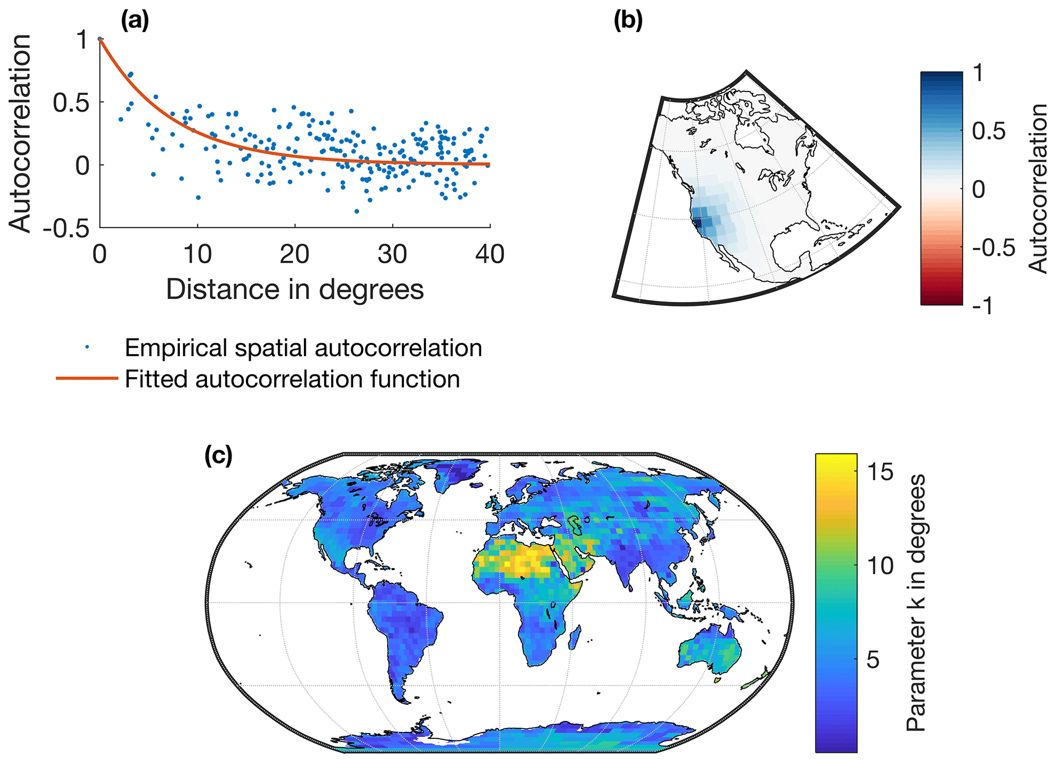
Figure 3Illustration of the spatial autocorrelation of the empirical model residuals and their representation in the SAR model (for the GRACE-REC product based on MSWEP and calibrated with JPL mascons). (a) Empirical and fitted spatial autocorrelation functions for the model residuals at a given mascon in California. (b) Fitted spatial autocorrelation at that mascon. (c) Fitted parameter k (Eq. 11), which conditions the steepness of the autocorrelation function (high values are equal to high autocorrelation length of the residuals).
As mentioned in Sect. 2.3, the Markov chain Monte Carlo (MCMC) procedure for model parameter estimation additionally provides a distribution of equally acceptable model parameters (a, b, and β). Each parameter set provides one ensemble member for which the entire procedure described here is repeated. Thus, ensemble members combine (1) a model parameter uncertainty arising from the distribution of calibrated model parameters and (2) an estimate of the predictive uncertainty. Here, we provide 100 randomly sampled ensemble members. This number was chosen as a compromise between the size of the final dataset and the minimum number of ensemble members required to derive a reasonable estimate of the 90 % confidence interval.
2.4.3 Evaluation of ensemble members
The result of the above-described procedure is briefly illustrated and evaluated in Fig. 4. For illustration, Fig. 4a shows the empirical residuals (ε) for the month of April 2002 and Fig. 4b shows one instance of the randomly generated residuals . As expected, both the empirical and the randomly generated residuals exhibit spatial autocorrelation. The generated residuals also have approximately the same variance (Fig. 4c) and lag-1 temporal autocorrelation (Fig. 4d) as that of the empirical residuals. The confidence intervals derived at a regional- or basin-scale level reliably cover the actual GRACE-based regional average, which was the initial motivation for the presented approach (illustrated for the Mississippi basin in Fig. 4e). We evaluate the overall reliability of the ensemble hindcast for regional averages over 90 large (>500 000 km2) river basins using a rank histogram (or Talagrand diagram) (Fig. 4f). In the ideal case (perfect reliability), the observed TWS ranks lower than the pth percentile of the reconstruction only p percent of the time (for instance, GRACE observations should be lower than the fifth percentile of the reconstruction only 5 % of the time). According to this first-order metric (see, e.g., Hamill, 2001, for a discussion), we conclude that regional averages of the ensemble members provide reliable forecasts (Fig. 4f), with only a minor tendency to miss extreme positive TWS anomalies.
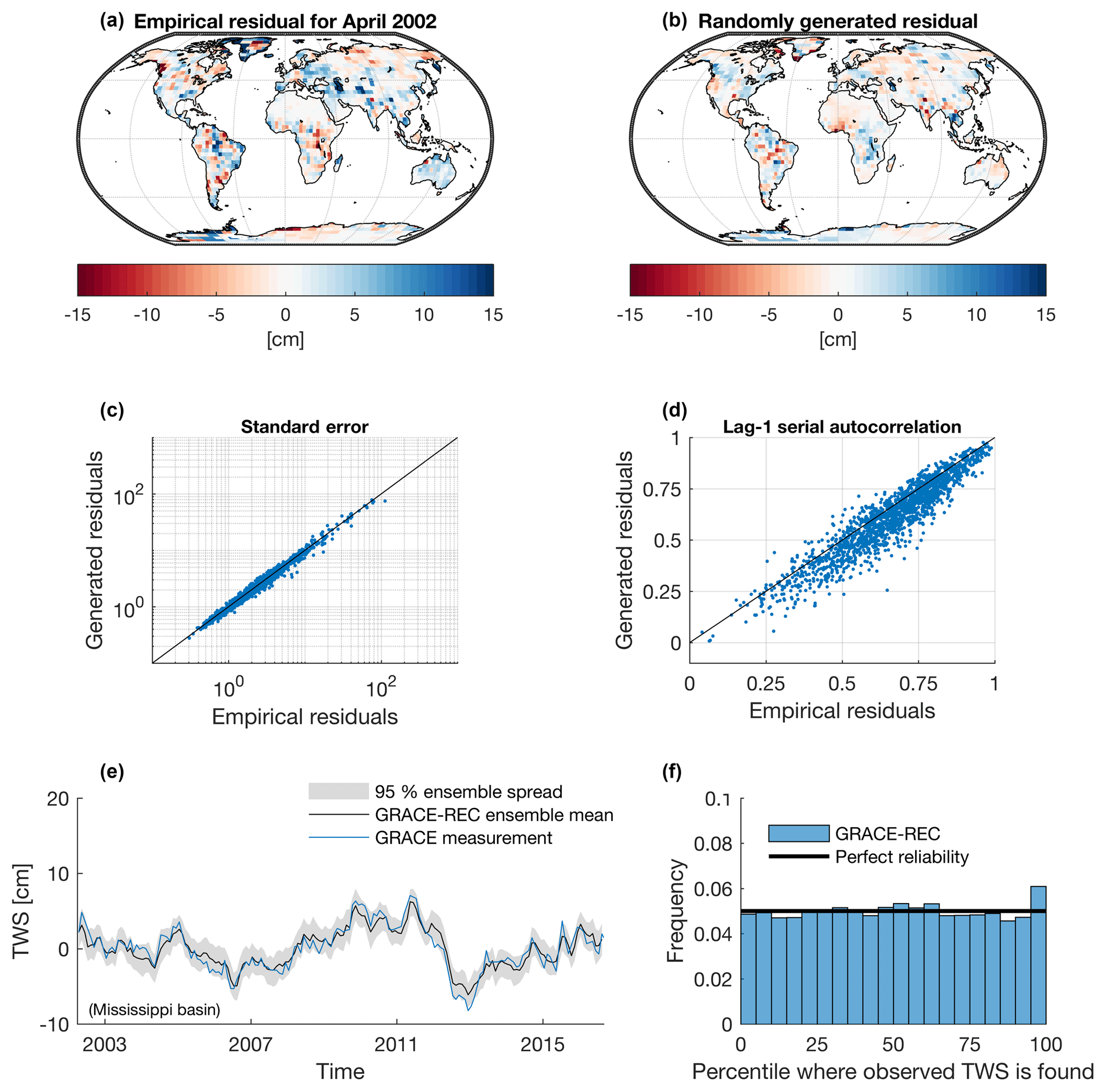
Figure 4Output of the SAR model for the generation of random noise realizations that have a spatiotemporal structure similar to that of the empirical model residuals (for the GRACE-REC product based on MSWEP and calibrated with JPL mascons). (a) Empirical model residual at a given time step. (b) Residual randomly generated by the SAR model. (c) Agreement between the standard deviation of the empirical versus generated residuals (each point represents one mascon). (d) Agreement between the lag-1 autocorrelation of the empirical versus generated residuals (each point represents one mascon). (e) Illustration of the resulting ensemble spread for a basin-scale average. (f) Rank histogram using 5 % bins, combining the data for 90 large (>500 000 km2) basins (from 2003 to 2014), used to evaluate the reliability of ensemble forecasts.
The presented method represents one amongst many possible approaches to the generation of ensemble members. This method has the advantage of reflecting the uncertainty of the reconstruction (compared to GRACE measurements) and mimics the empirical spatiotemporal autocorrelation structure of the errors while only requiring a minimal degree of model complexity and parameterization. We note that while the SAR model also represents errors coming from the GRACE solution itself, it does not include any anisotropic error structure (e.g., due to striping) due to the isotropic nature of Eq. (11). The uncertainty related to the choice of the input precipitation or training GRACE dataset can be explored independently by comparing the six different versions of GRACE-REC (see Table 3).
Table 3List of the six GRACE-REC datasets available at monthly and daily scales.
Finally, we note that our modeling approach could in principle be evaluated with a cross-validation experiment, using only a subset of the data to calibrate the model parameters and then evaluate the performance against the other unused data (as done in Humphrey et al., 2017). However, this would go beyond the scope and objective of this paper, which is to document the generation of the GRACE-REC product. We prefer to evaluate the ability of the final product to extrapolate beyond the model calibration period in later sections by comparing the model predictions with fully independent datasets (Sect. 4.3 to 4.5).
3.1 Definition of GRACE-REC TWS datasets
The GRACE-REC data provide de-seasonalized terrestrial water storage (TWS) anomalies in units of millimeters of water (kg m−2) (Eq. 8). Thus, GRACE-REC does not include a reconstructed seasonal TWS cycle. Because some applications also require the seasonal signals, we provide the GRACE-based TWS seasonal cycle (Humphrey et al., 2017), which can directly be added to the GRACE-REC TWS anomalies if needed. As a caveat, note that this GRACE-based TWS seasonal cycle is kept constant over time, which might potentially be unrealistic (Hamlington et al., 2019).
3.2 Monthly products with ensemble members
Using two different training GRACE datasets (Table 1) and three different precipitation forcing datasets (Table 2), we produce a total of six different GRACE-REC datasets with 100 ensemble members each. For convenience, we also provide smaller summary files which only contain the ensemble mean and 90 % confidence interval.
3.3 Daily products
For the daily TWS reconstructions, we only provide the ensemble mean of each GRACE-REC product in order to limit the data size. This ensemble mean is based on ensemble members which sample the parameter uncertainty only (Sect. 2.3.2). The reason for this is that no SAR model (Sect. 2.4.2) can be reliably calibrated at daily resolution as the two training GRACE datasets have monthly resolution. The format is identical to that of the monthly data (Table 3).
3.4 Global land averages
For global-scale applications, we provide global averages of the TWS time series. Global averages are weighted by mascon area and include all land mascons with or without Greenland and Antarctica (both options are available). This format is especially suited for sea level and global water budget studies and units are gigatons of water. To convert gigatons back to millimeters of global land water, total land area values of 148 940 000 and 132 773 914 km2 can be used for each option, respectively. The evaluation of global means in Sect. 4.1.2 and 4.3 can guide the choice between the different versions of GRACE-REC.
3.5 Interpretation of multi-decadal trends
Although linear trends are removed during model calibration (Eq. 6), potential TWS trends caused by decadal variability and long-term changes in precipitation are not removed from the final dataset (Eq. 8) and can be substantial. By definition, any trend found in the reconstructed TWS products is caused by a trend in the underlying precipitation forcing (since the time-varying residence time uses de-trended temperature and there is no limit to storage capacity). Thus the reconstructed TWS trends mainly depend on the trends initially present in the driving precipitation data (see Sect. 4.1.2 for an example at global scale).
With these elements in mind, it should be clear that there will be differences between the trends found in GRACE and the trends found in the reconstruction. Such discrepancies are expected because the reconstruction does not represent several sources of long-term changes in TWS, including for instance, land ice melt, dams, anthropogenic water depletion (Reager et al., 2016; Felfelani et al., 2017; Rodell et al., 2018), or long-term changes in evaporative demand. Consequently, trends in GRACE-REC cannot be directly evaluated against the trends from GRACE itself. Thus, when we compute trends over the period 2003–2014 (Figs. S2 and S3 in the Supplement), we find that reconstructed trends are consistent with GRACE trends only over certain regions, likely due to the reasons mentioned above (linear trends simulated by the WRR2 models are also shown in Fig. S4).
As illustrated in Humphrey et al. (2017), the reconstruction can be used to remove the precipitation-driven variability from the original GRACE time series in order to better isolate and quantify other sources of long-term changes (such as anthropogenic impacts). However, users interested in computing long-term TWS trends from this dataset should always proceed with caution as the dataset was not evaluated for trends. For regional analyses, we recommend using the model ensembles to obtain a range of possible trends and thus better assess the uncertainty. More generally, we highlight that the quality of the reconstruction is strongly dependent on the quality of the input precipitation forcing and on the adequateness of an exponential decay model for representing water storage behavior. For instance, routing of water through the river system is not represented and might be important over certain regions. Section 4.1 provides global maps of model performance that can guide regional applications.
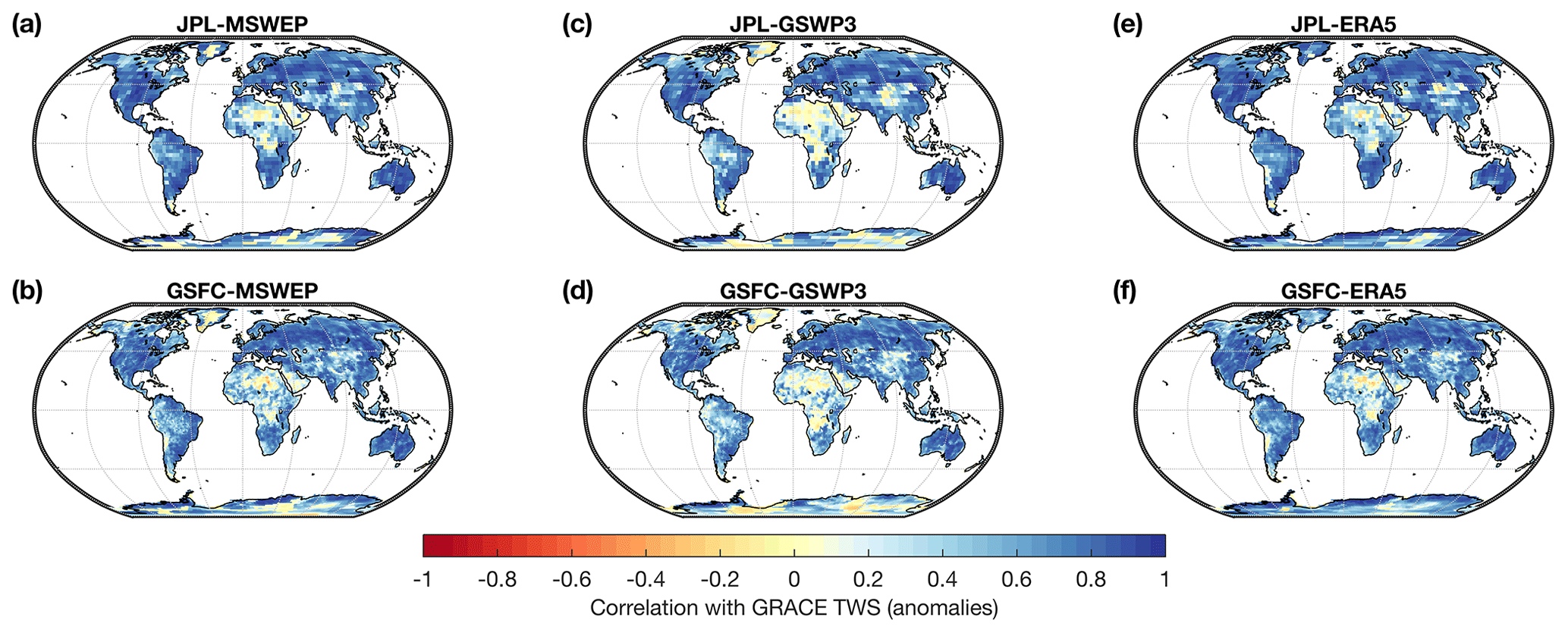
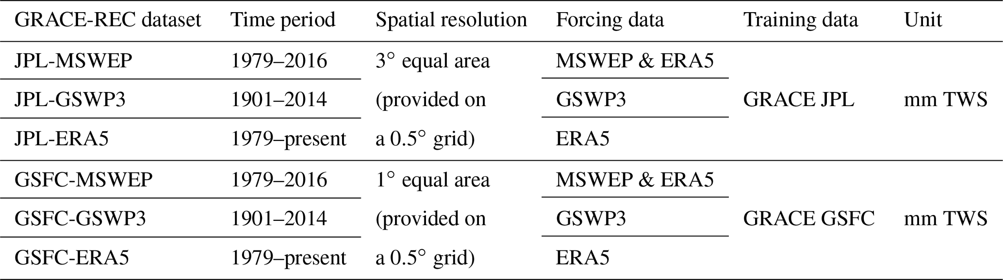
Figure 5Correlation (of de-seasonalized, de-trended anomalies) between GRACE-REC and GRACE JPL mascons (a, c, e) or GRACE GSFC mascons (b, d, f). Three different precipitation forcing datasets are tested: MSWEP (a, b), GSWP3 (c, d), and ERA5 (e, f). Values closer to 1 correspond to a higher model performance.
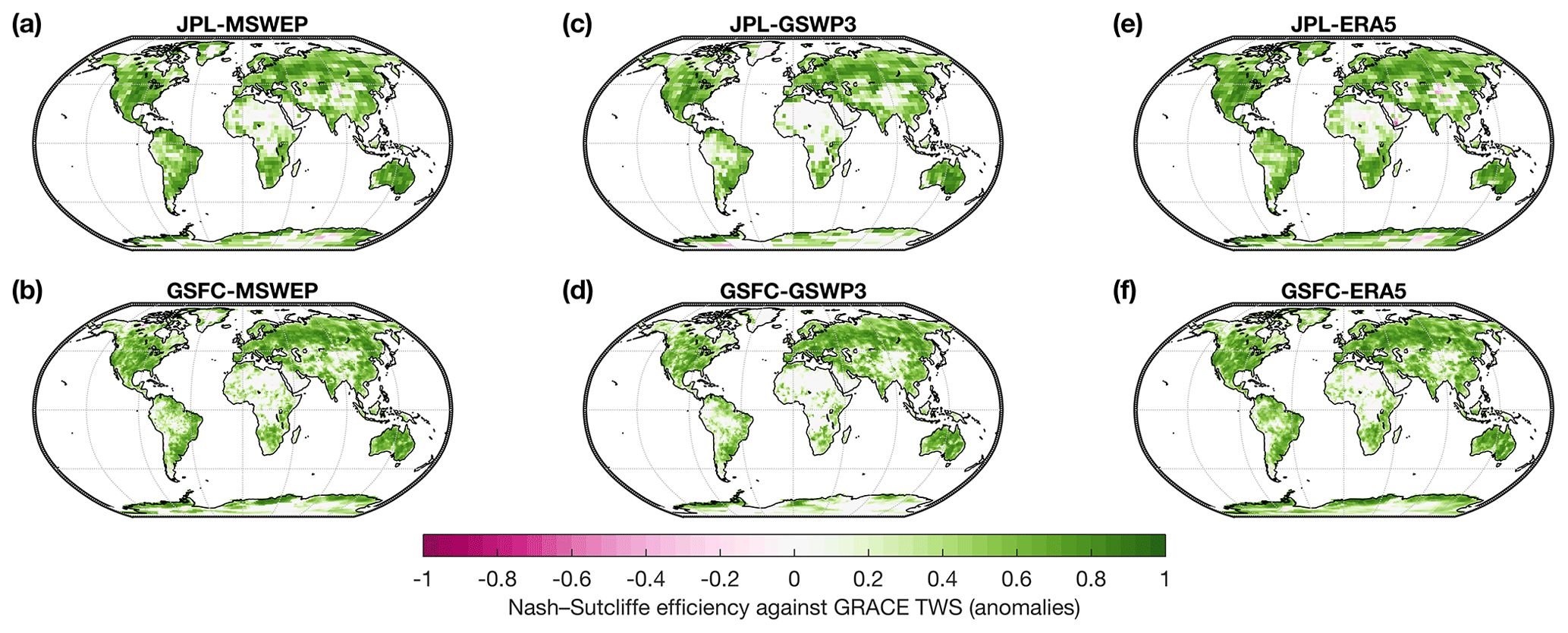
Figure 6Nash–Sutcliffe efficiency (of de-seasonalized, de-trended anomalies) between GRACE-REC and GRACE JPL mascons (a, c, e) or GRACE GSFC mascons (b, d, f). Three different precipitation forcing datasets are tested: MSWEP (a, b), GSWP3 (c, d), and ERA5 (e, f). Values closer to 1 correspond to a higher model performance.
4.1 Comparison with de-seasonalized monthly GRACE
4.1.1 Mascon scale
In this section, the ensemble mean of GRACE-REC is compared against GRACE observations. Note that this does not constitute an independent evaluation because GRACE-REC is calibrated with GRACE data (comparisons with independent sources are provided in Sect. 4.3 to 4.5). We evaluate model performance with the Pearson correlation coefficient (Fig. 5) and the Nash–Sutcliffe efficiency (Fig. 6). Model performance is highest especially in regions with dense meteorological observing systems (e.g., Europe, western Russia, North America, India, Australia) where we expect precipitation datasets to have the highest accuracy. Over South America and central Africa, the performance of the century-long reconstruction (GSWP3-based products, Figs. 5c, d and 6c, d) is slightly inferior to that of multisource and reanalysis precipitation datasets such as MSWEP and ERA5. Interestingly, there is no clear difference in performance when GRACE-REC is calibrated with the 3∘ JPL mascons (top row) or the 1∘ GSFC mascons (bottom row). We conclude that in terms of model performance, the choice of the GRACE product used to calibrate GRACE-REC is of secondary importance compared to the accuracy of the input precipitation datasets.
We compare these performance metrics with the scores obtained by hydrological models and land surface models of the Water Resources Reanalysis version 2 (WRR2) (Schellekens et al., 2017; Dutra et al., 2017), which were also forced with MSWEP precipitation. Compared to the simple modeling approach used in GRACE-REC, WRR2 models are forced with additional meteorological information (such as radiation and humidity), were calibrated using various data streams, sometimes including GRACE observations (Dutra et al., 2017; Decharme et al., 2011, 2012, 2016; Vergnes et al., 2014; Krinner et al., 2005; de Rosnay et al., 2002; Van Der Knijff et al., 2010; Döll et al., 2009; Sutanudjaja et al., 2011, 2014; van Beek and Bierkens, 2008; van Beek et al., 2011; Wada et al., 2011, 2014; van Dijk et al., 2013, 2014), and are potentially able to resolve more complex processes that are relevant for TWS, such as snow dynamics, the effect of vegetation phenology on evapotranspiration, and runoff routing through the river system. We calculate TWS in WRR2 models by summing over all simulated water reservoirs (this includes soil moisture, snow, groundwater, and surface waters whenever these are represented in the models). It is important to underline that unlike WRR2 models, GRACE-REC is directly calibrated to reproduce GRACE observations. Therefore, GRACE-REC should be interpreted here as a benchmark, indicative of the performance that is at least achievable for a given precipitation dataset. In terms of Nash–Sutcliffe efficiency, GRACE-REC often obtains better scores than the WRR2 models (Fig. 7a). This is because the reconstruction better fits the local amplitude and variance of the observed TWS signal, as already diagnosed in previous work (Humphrey et al., 2017). We note that the reconstructions driven with ERA5 precipitation are most often superior to those driven with the other two precipitation datasets.

Figure 7Global-area-weighted box plots of the performance metrics shown in Figs. 5 and 6 for GRACE-REC datasets (blue), and comparison with the performance of global hydrological models participating in the Earth2Observe Water Resources Reanalysis version 2 (WRR2) (orange). Dark colors indicate the performance obtained when comparing against JPL mascons, and against GSFC mascons for light colors. Note that WRR2 models are driven with MSWEP precipitation and all model outputs are aggregated to the resolution of the corresponding GRACE dataset. Greenland and Antarctica are always excluded.
4.1.2 Global scale
Global averages of all GRACE-REC products are illustrated in Fig. 8a. Differences caused by different precipitation forcing datasets are much greater than the differences related to different GRACE training datasets. This is particularly true for long-term (>20 years) trends as we find that, over the overlapping period 1979–2014, the two MSWEP-based products both produce a positive climate-driven TWS trend while GSWP3-based and ERA5-based products yield a negative TWS trend. As mentioned above (see Sect. 3.5), discrepancies in long-term trends in GRACE-REC largely depend on the trends initially present in the driving precipitation data and also do not incorporate effects such as groundwater depletion or potential long-term changes in evaporative demand.

Figure 8(a) Global average of TWS anomalies for the six GRACE-REC datasets (excluding Greenland and Antarctica) with an artificial vertical offset added for better visual comparison. (b) Comparison of the three GRACE-REC datasets calibrated with GRACE JPL against GRACE JPL (de-trended anomalies). (c) Same as (b) but for GRACE GSFC.
Comparisons with the de-trended GRACE global average are shown in Fig. 8b, c. We find that all GRACE-REC products produce a very similar inter-annual variability at the global scale and compare well against actual global mean GRACE, without applying any global constraint to the locally calibrated statistical model. Correlations between global means of GRACE-REC and global means of GRACE are larger than 0.75 (Fig. 9a) (evaluated over the common period 2003–2014). Compared to global means from the WRR2 models, GRACE-REC is on average better correlated (Fig. 9a) to the observed GRACE global mean and has a lower root-mean-square error (Fig. 9b), regardless of the GRACE dataset used for evaluation.
Figure 9Agreement of the global average of different TWS model estimates (from GRACE-REC, blue, and WRR2 models, orange) with the observed TWS anomalies from JPL (squares) and GSFC (crosses) solutions.
4.2 Comparison with de-seasonalized daily GRACE
We compare the daily GRACE-REC products with a Kalman smoothed daily GRACE solution named ITSG-Grace2018 (Kurtenbach et al., 2012; Mayer-Gürr et al., 2018). While this daily GRACE solution contains significant information on the sub-monthly variability of TWS, the increased temporal resolution is at the cost of spatial resolution, which is on the order of 500 km for this particular product (note that the solution is also correlated in time as a result of the Kalman smoothing). As illustrated in Fig. 10a, there can be a good agreement between GRACE-REC and ITSG-Grace2018 for sub-monthly variability when daily averages are computed over large regions (here the Mississippi basin). Figure 10b, c provide a summary of the agreement between GRACE-REC and ITSG-Grace2018 at a daily scale, as well as a comparison with the performance of WRR2 models. Due to the coarse resolution of the ITSG-Grace2018 product, the comparison (Fig. 10b, c) is conducted at a spatial resolution of 5∘. We find that, even though the performance of all products is lower than at monthly resolution, the GRACE-REC products agree on average as well as or better with ITSG-Grace2018 than most models of the WRR2 ensemble.
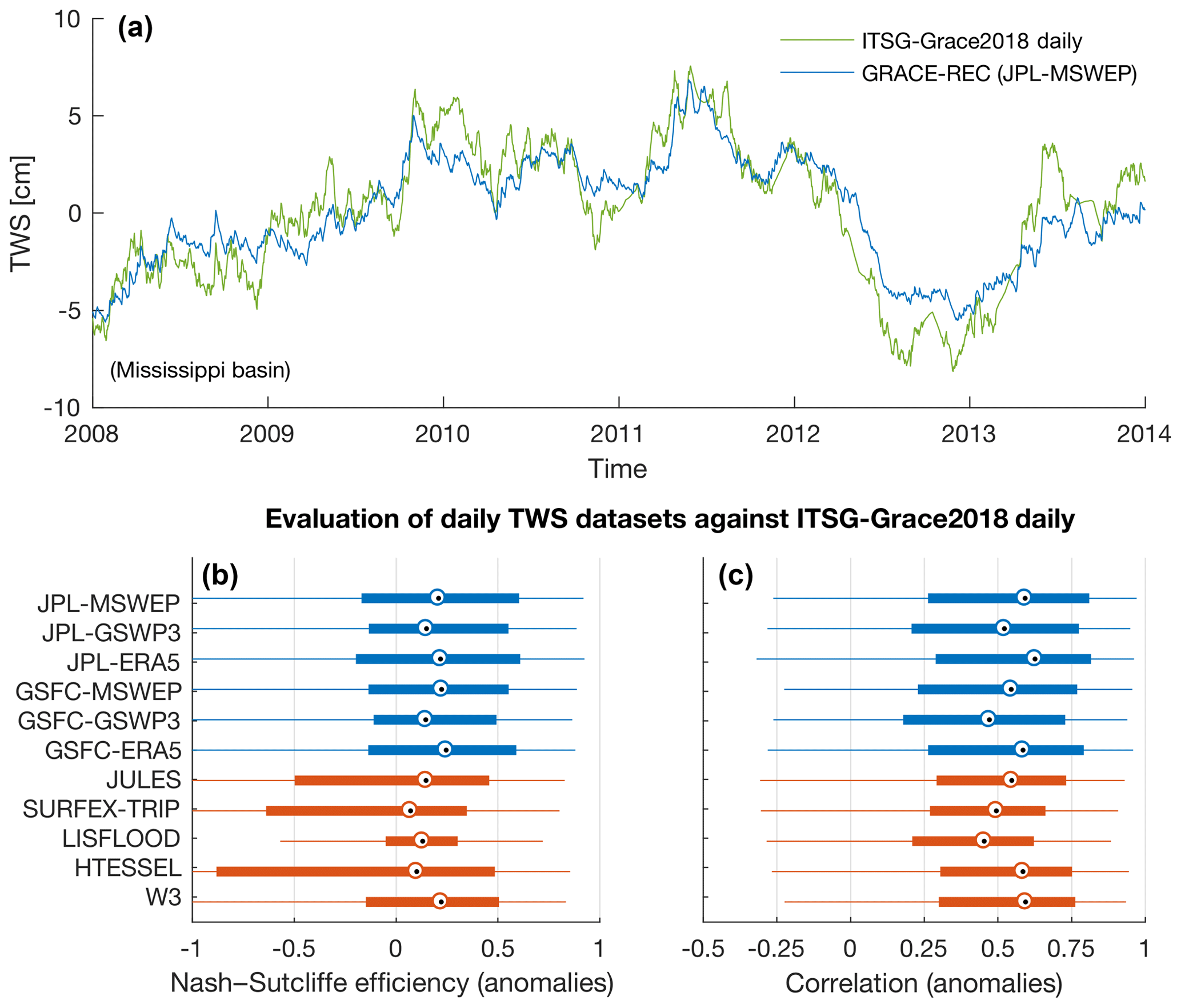
Figure 10(a) Comparison between the GRACE-REC daily TWS reconstruction (JPL-MSWEP dataset) and the daily GRACE ITSG-Grace2018 solution for the Mississippi basin (focused over the period 2008–2014 to improve readability of the high-frequency fluctuations). (b–c) Global-area-weighted box plots of the performance metrics of the daily TWS datasets when compared with ITSG-Grace2018 at a spatial resolution of 5∘. Note that some WRR2 models are not included because not all water storage variables were available to us at daily frequency. Greenland and Antarctica are excluded.
4.3 Comparison with the de-seasonalized and de-trended sea level budget
Together with changes in ocean heat content, changes in the amount of water stored on land are responsible for a large fraction of the year-to-year variability in global mean sea level (Boening et al., 2012; Cazenave et al., 2014; WCRP Global Sea Level Budget Group, 2018). Because changes in land water storage result in opposite changes in ocean mass, the sea level budget provides an independent mean of evaluating various estimates of global mean TWS variability. Here we assess the ability of terrestrial water storage products (GRACE, GRACE-REC, and the WRR2 models) to close the sea level budget at the inter-annual timescale. We use de-seasonalized and de-trended global mean sea level (GMSL) from satellite altimetry (Beckley et al., 2017) and steric height estimates (GMSLsteric) based on observations of Argo floats (Roemmich and Gilson, 2009; Llovel et al., 2014). From the sea level budget, we obtain an estimate of inter-annual changes in ocean mass (Eq. 16, black line in Fig. 11a), which we compare against global mean TWS estimates. We use this budget-based ocean mass to provide an independent evaluation of all TWS products (i.e., not based on any GRACE data), although GRACE-based ocean mass is obviously also available since 2002 (e.g., Watkins et al., 2015). Greenland and Antarctica are excluded from the TWS averages to enable a consistent comparison among all products (hydrological models typically do not represent these regions).
We find that, although all considered products are significantly correlated with the budget-based ocean mass (GMSLocean mass), GRACE and GRACE-REC estimates are clearly better correlated and yield a lower root-mean-square error (Fig. 11b, c). Surprisingly, GRACE-REC products also yield better results than the two original GRACE datasets (JPL and GSFC). We hypothesize that this might occur because the global mean GRACE TWS is more susceptible to non-compensating continental-scale errors (e.g., caused by errors in low-degree spherical harmonics or residual longitudinal stripes) compared to climate-driven reconstructions, which yield smoother global averages (as seen in Fig. 8b, c).
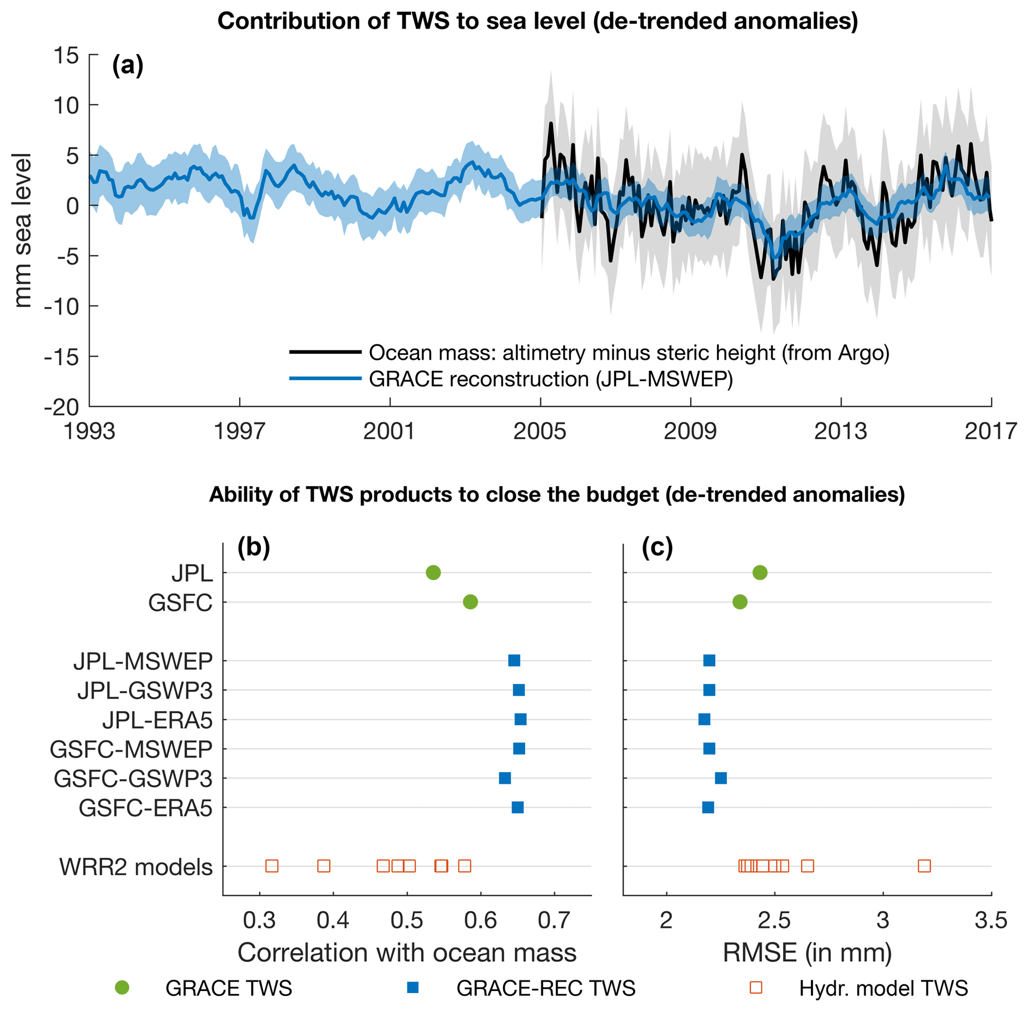
Figure 11(a) Comparison of the global mean TWS reconstructed by GRACE-REC (converted to equivalent mm sea level) against the ocean mass derived from the sea level budget. (b–c) Evaluation of the ability of various TWS datasets to close the sea level budget (GRACE estimates in green, GRACE-REC datasets in blue, and WRR2 models in orange).
4.4 Comparison with de-seasonalized basin-scale water balance
Over moderately large river basins (>100 000 km2), TWS changes can be estimated by combining streamflow measurements with moisture fluxes from an observation-assimilating atmospheric reanalysis system (Oki et al., 1995; Seneviratne et al., 2004). This approach provides relatively independent estimates of TWS changes over large basins, which has been used to evaluate distributed hydrological models and land surface models. Here, we aim to use such estimates to also evaluate the quality of the reconstruction during the period when no GRACE data are available (i.e., prior to 2002).
We evaluate TWS products using a recently updated basin-scale water balance dataset (BSWB) (Hirschi and Seneviratne, 2017), which covers 341 catchments and is based on ERA-Interim reanalysis data (Dee et al., 2011) and runoff observations from the Global Runoff Data Centre (GRDC). The temporal coverage of BSWB estimates at each river basin thus depends on the availability of runoff data and does not always cover the GRACE time period. As a caveat, we note that BSWB should not be viewed as entirely independent of WRR2 models or as a ground truth. This is because moisture fluxes from ERA-Interim are not only influenced by the assimilated atmospheric profile information but are also dependent on the underlying land surface model (TESSEL), which is similar to WRR2 models in many aspects. All WRR2 models also used ERA-Interim as forcing data for all meteorological variables except for precipitation.
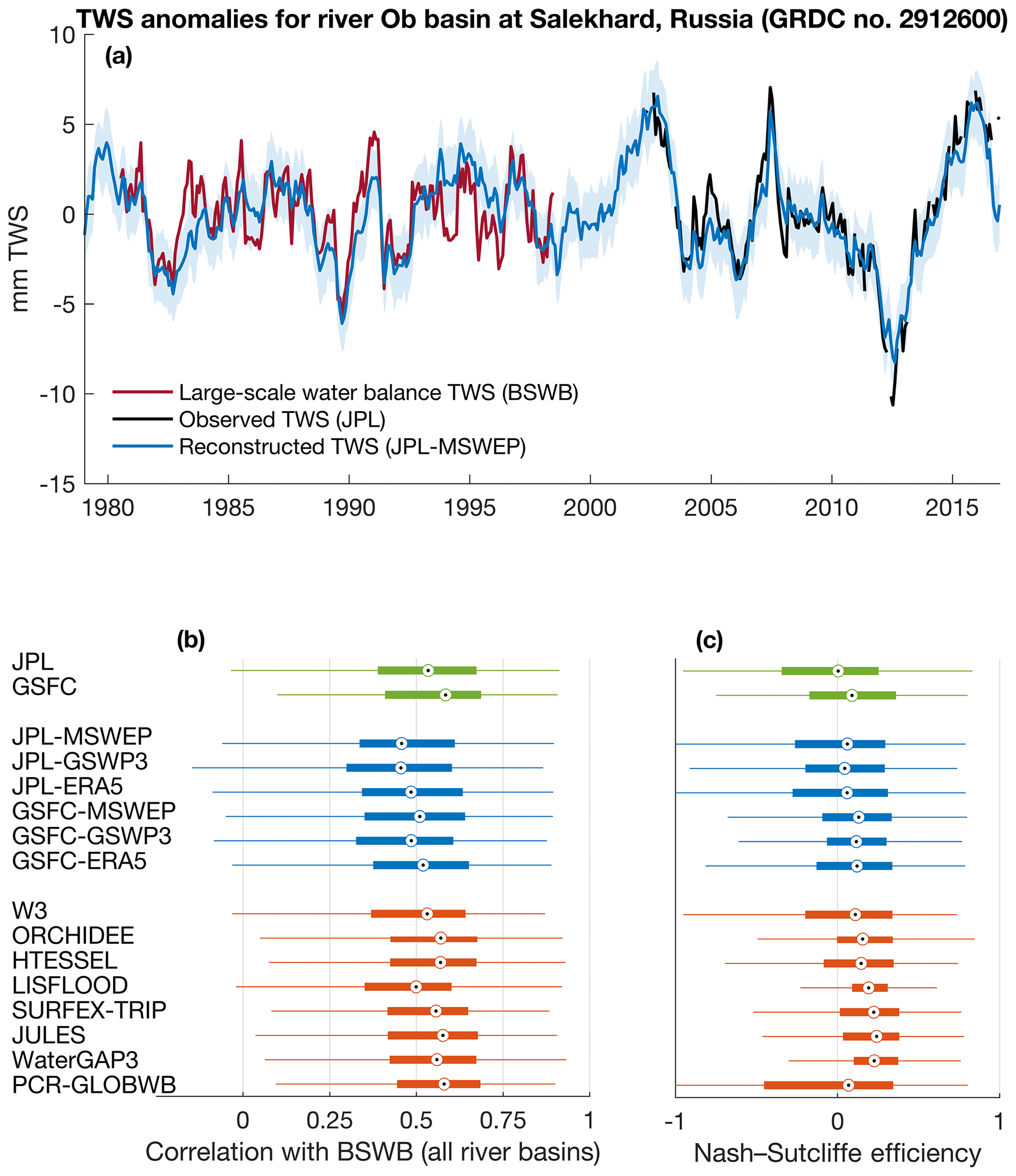
Figure 12(a) Comparison between TWS anomalies derived from atmospheric basin-scale water balance (BSWB), GRACE observations (JPL), and the GRACE reconstruction (JPL-MSWEP dataset). (b–c) Global box plots of the agreement between various TWS products and BSWB estimates (based on the performance metrics at 341 large basins). The scale factors were applied to the JPL data for this specific analysis.
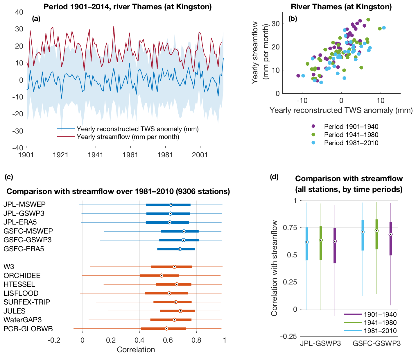
Figure 13(a) Comparison between century-long measurements of streamflow and the TWS anomalies reconstructed at this location (GSFC-GSWP3 dataset). (b) Scatter plot of the data in (a), by time period. (c) Global box plots of the performance of GRACE-REC and WRR2 models when compared with yearly streamflow anomalies. (d) Global box plots of the performance of the JPL-GSWP3 and GSFC-GSWP3 products when compared with yearly streamflow anomalies, by time period (n=1274, 8065, and 9306 for 1901–1940, 1941–1980, and 1981–2010 respectively).
As illustrated in Fig. 12a for the Ob basin, we find that the reconstructed TWS compares relatively well with BSWB estimates. Overall, all TWS products considered here (including the GRACE data) seem to compare relatively well with BSWB (Fig. 12b, c). We note that GRACE-REC products calibrated on GSFC seem to compare slightly better with BSWB than the JPL-based products. This might be because of the higher spatial sampling of the GSFC mascons (1∘ instead of 3∘ for JPL), which might enable a better separation between mass changes located inside or outside the river basin boundaries. This mainly occurs because the meteorological forcing is aggregated at a resolution of 1∘ in the case of GSFC-based products, allowing the GSFC reconstructions to provide a slightly more localized signal.
4.5 Comparison with annual streamflow measurements
In this section, we compare reconstructed TWS against streamflow observations over the period 1901 to 2010. Streamflow and TWS of course represent different variables with different units; however, we expect that their temporal dynamics will correlate at the yearly scale, as illustrated for the river Thames in Fig. 13a, b. Because observed streamflow is one of the few water cycle variables available prior to 1980, it provides an independent and useful means of evaluating the century-long reconstruction. We use streamflow observations collected by the Global Streamflow Indices and Metadata Archive (GSIM) (Do et al., 2018a; Gudmundsson et al., 2018). From the 30 959 available stations, we keep stations with a basin size smaller than 10 000 km2 and with at least 10 years of available data (discarding any year where less than 50 % of the daily values were available to compute the yearly mean), leaving 12 496 stations for analysis. The reason for focusing on small basins is that a much larger number of them are available in the early century (compared to the number of large basins, which are the focus of Sect. 4.4). We note that the unavoidable mismatch in resolution between large-scale mass changes and local catchment runoff dynamics is to some extent alleviated by the spatial coherence of yearly anomalies in weather patterns.
We find that TWS anomalies from both WRR2 models and GRACE-REC compare well with yearly streamflow variability over the period 1980–2010 (Fig. 13c). Reconstructions based on the GSFC products tend to perform slightly better, again likely because of their higher spatial sampling (1∘) compared to the JPL-based reconstructions (3∘). When evaluating the century-long reconstruction (GSWP3-driven products), we find that the correlation between yearly TWS anomalies and yearly runoff only slightly degrades for the earliest time period (1901–1940) but is otherwise relatively stable over time (Fig. 13d). This indicates that, even though GRACE-REC was calibrated over the years 2002–2016, the model is still able to reproduce past water cycle variability and does not overfit to the period of the GRACE mission. In addition, we note that the quality of the century-long reconstruction is of course dependent on the accuracy of the GSWP3 precipitation and temperature forcing, which likely degrades towards the beginning of the century as fewer observations are available.
The presented dataset is publicly available (https://doi.org/10.6084/m9.figshare.7670849, Humphrey and Gudmundsson, 2019) and updates of the two reconstructions driven by ERA5 will be published when needed. We note that because including additional GRACE months only barely improves the quality of the model fit, no systematic recalibration of the models is planned at this stage. The data can be freely used provided this paper is acknowledged.
All datasets used in this paper are available at the following locations: GSWP3 (https://doi.org/10.20783/DIAS.501), GRACE JPL mascons (https://grace.jpl.nasa.gov/data/get-data/jpl_global_mascons/, last access: 18 July 2019), GRACE GSFC (https://neptune.gsfc.nasa.gov/gngphys/index.php?section=470, last access: 18 July 2019), MSWEP V2 (http://www.gloh2o.org/, last access: 18 July 2019), ERA5 (https://cds.climate.copernicus.eu/\#!/search?text=ERA5&type=dataset, last access: 18 July 2019), ITSG-Grace2018 (http://icgem.gfz-potsdam.de/series, last access: 18 July 2019), NASA Sea Level Change Portal (https://sealevel.nasa.gov/, last access: 18 July 2019), BSWB (https://doi.org/10.5905/ethz-1007-82, Hirschi and Seneviratne, 2016), GRDC Reference Dataset (https://www.bafg.de/GRDC, last access: 18 July 2019), GSIM (https://doi.org/10.1594/PANGAEA.887477, Do et al., 2018b), WRR2 (http://wci.earth2observe.eu/thredds/catalog-earth2observe-model-wrr2.html, last access: 18 July 2019), and the Earth2Observe project (http://www.earth2observe.eu/, last access: 18 July 2019).
We present a statistical reconstruction of climate-driven terrestrial water storage changes at daily and monthly resolution in six different configurations which cover three different time periods (Table 3). We evaluate the performance of this reconstruction and show that its overall accuracy is reasonable compared to other estimates of TWS variability available from global hydrological models. We also highlight the versatility and robustness of our approach by comparing our estimates with independent observations of Earth system variables outside of the calibration period.
The supplement related to this article is available online at: https://doi.org/10.5194/essd-11-1153-2019-supplement.
VH and LG developed the approach. VH performed the analyses, produced the dataset and wrote the paper with feedback from LG.
The authors declare that they have no conflict of interest.
We thank Sonia Seneviratne for critical feedback and support of this work. We thank Hyungjun Kim for developing the GSWP3 forcing and providing us with early access to the data. We thank Richard Wartenburger for technical support. Model developers and data providers are also gratefully acknowledged for sharing their data.
This research has been supported by the European Research Council (DROUGHT-HEAT (grant no. 617518)) and by the Swiss National Science Foundation (grant no. P400P2_180784).
This paper was edited by Christian Voigt and reviewed by three anonymous referees.
A, G., Wahr, J., and Zhong, S.: Computations of the viscoelastic response of a 3-D compressible Earth to surface loading: an application to Glacial Isostatic Adjustment in Antarctica and Canada, Geophys. J. Int., 192, 557–572, https://doi.org/10.1093/gji/ggs030, 2013.
Adhikari, S. and Ivins, E. R.: Climate-driven polar motion: 2003–2015, Science Advances, 2, e1501693, https://doi.org/10.1126/sciadv.1501693, 2016.
Anderegg, W. R. L., Konings, A. G., Trugman, A. T., Yu, K., Bowling, D. R., Gabbitas, R., Karp, D. S., Pacala, S., Sperry, J. S., Sulman, B. N., and Zenes, N.: Hydraulic diversity of forests regulates ecosystem resilience during drought, Nature, 561, 538–541, https://doi.org/10.1038/s41586-018-0539-7, 2018.
Andrew, R., Guan, H., and Batelaan, O.: Estimation of GRACE water storage components by temporal decomposition, J. Hydrol., 552, 341–350, https://doi.org/10.1016/j.jhydrol.2017.06.016, 2017.
Beck, H. E., van Dijk, A. I. J. M., Levizzani, V., Schellekens, J., Miralles, D. G., Martens, B., and de Roo, A.: MSWEP: 3-hourly 0.25∘ global gridded precipitation (1979–2015) by merging gauge, satellite, and reanalysis data, Hydrol. Earth Syst. Sci., 21, 589–615, https://doi.org/10.5194/hess-21-589-2017, 2017.
Beck, H. E., Wood, E. F., Pan, M., Fisher, C. K., Miralles, D. G., van Dijk, A. I. J. M., McVicar, T. R., and Adler, R. F.: MSWEP V2 global 3-hourly 0.1∘ precipitation: methodology and quantitative assessment, B. Am. Meteorol. Soc., 100, 473–500, https://doi.org/10.1175/bams-d-17-0138.1, 2018.
Beckley, B. D., Callahan, P. S., Hancock, D. W., Mitchum, G. T., and Ray, R. D.: On the “Cal-Mode” Correction to TOPEX Satellite Altimetry and Its Effect on the Global Mean Sea Level Time Series, J. Geophys. Res.-Oceans, 122, 8371–8384, https://doi.org/10.1002/2017jc013090, 2017.
Beguería, S., Vicente-Serrano, S. M., Reig, F., and Latorre, B.: Standardized precipitation evapotranspiration index (SPEI) revisited: parameter fitting, evapotranspiration models, tools, datasets and drought monitoring, Int. J. Climatol., 34, 3001–3023, https://doi.org/10.1002/joc.3887, 2014.
Bento, V. A., Gouveia, C. M., DaCamara, C. C., and Trigo, I. F.: A climatological assessment of drought impact on vegetation health index, Agr. Forest Meteorol., 259, 286–295, https://doi.org/10.1016/j.agrformet.2018.05.014, 2018.
Beven, K. J.: Rainfall-Runoff Modelling: The Primer, 2nd edn., John Wiley & Sons, Chichester, 2012.
Bevington, P. R. and Robinson, D. K.: Data reduction and error analysis for the physical sciences, 3rd edn., McGraw-Hill, Boston, 320 pp., 2003.
Boening, C., Willis, J. K., Landerer, F. W., Nerem, R. S., and Fasullo, J.: The 2011 La Nina: So strong, the oceans fell, Geophys. Res. Lett., 39, L19602, https://doi.org/10.1029/2012GL053055, 2012.
Cazenave, A., Dieng, H. B., Meyssignac, B., von Schuckmann, K., Decharme, B., and Berthier, E.: The rate of sea-level rise, Nat. Clim. Change, 4, 358–361, https://doi.org/10.1038/nclimate2159, 2014.
Chambers, D. P., Cazenave, A., Champollion, N., Dieng, H., Llovel, W., Forsberg, R., von Schuckmann, K., and Wada, Y.: Evaluation of the Global Mean Sea Level Budget between 1993 and 2014, Surv. Geophys., 38, 309–327, https://doi.org/10.1007/s10712-016-9381-3, 2016.
Chao, B. F., Wu, Y. H., and Li, Y. S.: Impact of Artificial Reservoir Water Impoundment on Global Sea Level, Science, 320, 212–214, https://doi.org/10.1126/science.1154580, 2008.
Chen, J., Famiglietti, J. S., Scanlon, B. R., and Rodell, M.: Groundwater storage changes: present status from GRACE observations, Surv Geophys, 37, 397–417, https://doi.org/10.1007/s10712-015-9332-4, 2016.
Cheng, L., Trenberth, K. E., Fasullo, J., Boyer, T., Abraham, J., and Zhu, J.: Improved estimates of ocean heat content from 1960 to 2015, Science Advances, 3, e1601545, https://doi.org/10.1126/sciadv.1601545, 2017.
Compo, G. P., Whitaker, J. S., Sardeshmukh, P. D., Matsui, N., Allan, R. J., Yin, X., Gleason, B. E., Vose, R. S., Rutledge, G., Bessemoulin, P., Brönnimann, S., Brunet, M., Crouthamel, R. I., Grant, A. N., Groisman, P. Y., Jones, P. D., Kruk, M. C., Kruger, A. C., Marshall, G. J., Maugeri, M., Mok, H. Y., Nordli, Ø., Ross, T. F., Trigo, R. M., Wang, X. L., Woodruff, S. D., and Worley, S. J.: The Twentieth Century Reanalysis Project, Q. J. Roy. Meteor. Soc., 137, 1–28, https://doi.org/10.1002/qj.776, 2011.
Cressie, N. A. C. and Wikle, C. K.: Statistics for spatio-temporal data, Wiley series in probability and statistics, Wiley, Hoboken, N.J., 588 pp., 2011.
Dai, A. and Zhao, T.: Uncertainties in historical changes and future projections of drought. Part I: estimates of historical drought changes, Climatic Change, 144, 519–533, https://doi.org/10.1007/s10584-016-1705-2, 2016.
Decharme, B., Boone, A., Delire, C., and Noilhan, J.: Local evaluation of the Interaction between Soil Biosphere Atmosphere soil multilayer diffusion scheme using four pedotransfer functions, J. Geophys. Res., 116, D20126, https://doi.org/10.1029/2011JD016002, 2011.
Decharme, B., Alkama, R., Papa, F., Faroux, S., Douville, H., and Prigent, C.: Global off-line evaluation of the ISBA-TRIP flood model, Clim. Dynam., 38, 1389–1412, 2012.
Decharme, B., Brun, E., Boone, A., Delire, C., Le Moigne, P., and Morin, S.: Impacts of snow and organic soils parameterization on northern Eurasian soil temperature profiles simulated by the ISBA land surface model, The Cryosphere, 10, 853–877, https://doi.org/10.5194/tc-10-853-2016, 2016.
Dee, D. P., Uppala, S. M., Simmons, A. J., Berrisford, P., Poli, P., Kobayashi, S., Andrae, U., Balmaseda, M. A., Balsamo, G., Bauer, P., Bechtold, P., Beljaars, A. C. M., van de Berg, L., Bidlot, J., Bormann, N., Delsol, C., Dragani, R., Fuentes, M., Geer, A. J., Haimberger, L., Healy, S. B., Hersbach, H., Hólm, E. V., Isaksen, L., Kållberg, P., Köhler, M., Matricardi, M., McNally, A. P., Monge-Sanz, B. M., Morcrette, J. J., Park, B. K., Peubey, C., de Rosnay, P., Tavolato, C., Thépaut, J. N., and Vitart, F.: The ERA-Interim reanalysis: configuration and performance of the data assimilation system, Quarterly J. Roy. Meteor. Soc., 137, 553–597, https://doi.org/10.1002/qj.828, 2011.
de Rosnay, P., Polcher, J., Bruen, M., and Laval, K.: Impact of a physically based soil water flow and soil-plant interaction representation for modeling large-scale land surface processes, J. Geophys. Res., 107, 4118, https://doi.org/10.1029/2001JD000634, 2002.
Dieng, H. B., Cazenave, A., Meyssignac, B., and Ablain, M.: New estimate of the current rate of sea level rise from a sea level budget approach, Geophys. Res. Lett., 44, 3744–3751, https://doi.org/10.1002/2017gl073308, 2017.
Dill, R. and Dobslaw, H.: Numerical simulations of global-scale high-resolution hydrological crustal deformations, J. Geophys. Res.-Sol. Ea., 118, 5008–5017, https://doi.org/10.1002/jgrb.50353, 2013.
Do, H. X., Gudmundsson, L., Leonard, M., and Westra, S.: The Global Streamflow Indices and Metadata Archive (GSIM) – Part 1: The production of a daily streamflow archive and metadata, Earth Syst. Sci. Data, 10, 765–785, https://doi.org/10.5194/essd-10-765-2018, 2018a.
Do, H. X., Gudmundsson, L., Leonard, M., and Westra, S.: The Global Streamflow Indices and Metadata Archive – Part 1: Station catalog and Catchment boundary, PANGAEA, https://doi.org/10.1594/PANGAEA.887477, 2018b.
Döll, P., Fiedler, K., and Zhang, J.: Global-scale analysis of river flow alterations due to water withdrawals and reservoirs, Hydrol. Earth Syst. Sci., 13, 2413–2432, https://doi.org/10.5194/hess-13-2413-2009, 2009.
D'Orangeville, L., Maxwell, J., Kneeshaw, D., Pederson, N., Duchesne, L., Logan, T., Houle, D., Arseneault, D., Beier, C. M., Bishop, D. A., Druckenbrod, D., Fraver, S., Girard, F., Halman, J., Hansen, C., Hart, J. L., Hartmann, H., Kaye, M., Leblanc, D., Manzoni, S., Ouimet, R., Rayback, S., Rollinson, C. R., and Phillips, R. P.: Drought timing and local climate determine the sensitivity of eastern temperate forests to drought, Glob. Change Biol., 24, 2339–2351, https://doi.org/10.1111/gcb.14096, 2018.
Dutra, E., Balsamo, G., Calvet, J., Munier, S., Burke, S., Fink, G., van Dijk, A., Martinez-de la Torre, A., van Beek, R., and de Roo, A.: Report on the improved Water Resources Reanalysis, EartH2Observe, Report No.: D.5.2., 94 pp., 2017.
Eicker, A., Forootan, E., Springer, A., Longuevergne, L., and Kusche, J.: Does GRACE see the terrestrial water cycle “intensifying”?, J. Geophys. Res.-Atmos., 121, 733–745, 2016.
Fasullo, J. T., Lawrence, D. M., and Swenson, S. C.: Are GRACE-era Terrestrial Water Trends Driven by Anthropogenic Climate Change?, Adv. Meteorol., 2016, 4830603, https://doi.org/10.1155/2016/4830603, 2016.
Felfelani, F., Wada, Y., Longuevergne, L., and Pokhrel, Y. N.: Natural and human-induced terrestrial water storage change: A global analysis using hydrological models and GRACE, J. Hydrol., 553, 105–118, https://doi.org/10.1016/j.jhydrol.2017.07.048, 2017.
Frederikse, T., Jevrejeva, S., Riva, R. E. M., and Dangendorf, S.: A Consistent Sea-Level Reconstruction and Its Budget on Basin and Global Scales over 1958–2014, J. Climate, 31, 1267–1280, https://doi.org/10.1175/jcli-d-17-0502.1, 2018.
Gao, S., Liu, R., Zhou, T., Fang, W., Yi, C., Lu, R., Zhao, X., and Luo, H.: Dynamic responses of tree-ring growth to multiple dimensions of drought, Glob. Change Biol., 24, 5380–5390, https://doi.org/10.1111/gcb.14367, 2018.
Getirana, A., Kumar, S., Girotto, M., and Rodell, M.: Rivers and Floodplains as Key Components of Global Terrestrial Water Storage Variability, Geophys. Res. Lett., 44, 10359–310368, https://doi.org/10.1002/2017gl074684, 2017.
Griffin, D. and Anchukaitis, K. J.: How unusual is the 2012–2014 California drought?, Geophys. Res. Lett., 41, 9017–9023, https://doi.org/10.1002/2014gl062433, 2014.
Gudmundsson, L., Do, H. X., Leonard, M., and Westra, S.: The Global Streamflow Indices and Metadata Archive (GSIM) – Part 2: Quality control, time-series indices and homogeneity assessment, Earth Syst. Sci. Data, 10, 787–804, https://doi.org/10.5194/essd-10-787-2018, 2018.
Haario, H., Laine, M., Mira, A., and Saksman, E.: DRAM: Efficient adaptive MCMC, Stat. Comput., 16, 339–354, https://doi.org/10.1007/s11222-006-9438-0, 2006.
Hamill, T. M.: Interpretation of Rank Histograms for Verifying Ensemble Forecasts, Mon. Weather Rev., 129, 550–560, https://doi.org/10.1175/1520-0493(2001)129<0550:iorhfv>2.0.co;2, 2001.
Hamlington, B. D., Reager, J. T., Chandanpurkar, H., and Kim, K. Y.: Amplitude Modulation of Seasonal Variability in Terrestrial Water Storage, Geophys. Res. Lett., 46, 4404–4412, https://doi.org/10.1029/2019gl082272, 2019.
Hanasaki, N., Yoshikawa, S., Pokhrel, Y., and Kanae, S.: A global hydrological simulation to specify the sources of water used by humans, Hydrol. Earth Syst. Sci., 22, 789–817, https://doi.org/10.5194/hess-22-789-2018, 2018.
Haslinger, K. and Blöschl, G.: Space-Time Patterns of Meteorological Drought Events in the European Greater Alpine Region Over the Past 210 Years, Water Resour. Res., 53, 9807–9823, https://doi.org/10.1002/2017wr020797, 2017.
Heim, R. R.: A Comparison of the Early Twenty-First Century Drought in the United States to the 1930s and 1950s Drought Episodes, B. Am. Meteorol. Soc., 98, 2579–2592, https://doi.org/10.1175/bams-d-16-0080.1, 2017.
Hersbach, H. and Dee, D.: ERA5 reanalysis is in production, ECMWF newsletter, No. 147, 2016.
Hirschi, M. and Seneviratne, S. I.: BSWB v2016, Institute for Atmospheric and Climate Science, ETH Zürich, https://doi.org/10.5905/ethz-1007-82, 2016.
Hirschi, M. and Seneviratne, S. I.: Basin-scale water-balance dataset (BSWB): an update, Earth Syst. Sci. Data, 9, 251–258, https://doi.org/10.5194/essd-9-251-2017, 2017.
Huang, M., Wang, X., Keenan, T. F., and Piao, S.: Drought timing influences the legacy of tree growth recovery, Glob. Change Biol., 24, 3546–3559, https://doi.org/10.1111/gcb.14294, 2018.
Humphrey, V.: Terrestrial water storage: large-scale variability and the global carbon cycle, Diss ETH 24696, Zürich, 156 pp., 2017.
Humphrey, V. and Gudmundsson, L.: GRACE-REC: a reconstruction of climate-driven water storage changes over the last century, Dataset, figshare, https://doi.org/10.6084/m9.figshare.7670849, 2019.
Humphrey, V., Gudmundsson, L., and Seneviratne, S. I.: A global reconstruction of climate-driven subdecadal water storage variability, Geophys. Res. Lett., 44, 2300–2309, https://doi.org/10.1002/2017GL072564, 2017.
Humphrey, V., Zscheischler, J., Ciais, P., Gudmundsson, L., Sitch, S., and Seneviratne, S. I.: Sensitivity of atmospheric CO2 growth rate to observed changes in terrestrial water storage, Nature, 560, 628–631, https://doi.org/10.1038/s41586-018-0424-4, 2018.
Jacob, T., Wahr, J., Pfeffer, W. T., and Swenson, S.: Recent contributions of glaciers and ice caps to sea level rise, Nature, 482, 514–518, 2012.
Khaki, M., Forootan, E., Kuhn, M., Awange, J., van Dijk, A. I. J. M., Schumacher, M., and Sharifi, M. A.: Determining water storage depletion within Iran by assimilating GRACE data into the W3RA hydrological model, Adv. Water Resour., 114, 1–18, https://doi.org/10.1016/j.advwatres.2018.02.008, 2018.
Kim, H. J.: Global Soil Wetness Project Phase 3 Atmospheric Boundary Counditions (Experiment 1), Data Integration and Analysis System (DIAS), https://doi.org/10.20783/DIAS.501, 2017.
Krinner, G., Viovy, N., de Noblet-Ducoudre, N., Ogee, J., Polcher, J., Friedlingstein, P., Ciais, P., Sitch, S., and Prentice, I. C.: A dynamic global vegetation model for studies of the coupled atmosphere-biosphere system, Global Biogeochem. Cy., 19, GB1015,, https://doi.org/10.1029/2003GB002199, 2005.
Kurtenbach, E., Eicker, A., Mayer-Gürr, T., Holschneider, M., Hayn, M., Fuhrmann, M., and Kusche, J.: Improved daily GRACE gravity field solutions using a Kalman smoother, J. Geodyn., 59–60, 39–48, https://doi.org/10.1016/j.jog.2012.02.006, 2012.
Kusche, J., Eicker, A., Forootan, E., Springer, A., and Longuevergne, L.: Mapping probabilities of extreme continental water storage changes from space gravimetry, Geophys. Res. Lett., 43, 8026–8034, https://doi.org/10.1002/2016gl069538, 2016.
Llovel, W., Willis, J. K., Landerer, F. W., and Fukumori, I.: Deep-ocean contribution to sea level and energy budget not detectable over the past decade, Nat. Clim. Change, 4, 1031–1035, https://doi.org/10.1038/nclimate2387, 2014.
Luthcke, S. B., Sabaka, T. J., Loomis, B. D., Arendt, A. A., McCarthy, J. J., and Camp, J.: Antarctica, Greenland and Gulf of Alaska land-ice evolution from an iterated GRACE global mascon solution, J. Glaciol., 59, 613–631, https://doi.org/10.3189/2013JoG12J147, 2013.
Markonis, Y., Hanel, M., Máca, P., Kyselý, J., and Cook, E. R.: Persistent multi-scale fluctuations shift European hydroclimate to its millennial boundaries, Nat. Commun., 9, 1767, https://doi.org/10.1038/s41467-018-04207-7, 2018.
Mayer-Gürr, T., Behzadpour, S., Ellmer, M., Kvas, A., Klinger, B., Strasser, S., and Zehentner, N.: ITSG-Grace2018 – Monthly, Daily and Static Gravity Field Solutions from GRACE, GFZ DataServices, https://doi.org/10.5880/ICGEM.2018.003, 2018.
Moreira, D. M., Calmant, S., Perosanz, F., Xavier, L., Rotunno Filho, O. C., Seyler, F., and Monteiro, A. C.: Comparisons of observed and modeled elastic responses to hydrological loading in the Amazon basin, Geophys. Res. Lett., 43, 9604–9610, https://doi.org/10.1002/2016gl070265, 2016.
Ni, S., Chen, J., Wilson, C. R., Li, J., Hu, X., and Fu, R.: Global Terrestrial Water Storage Changes and Connections to ENSO Events, Surv. Geophys., 39, 1–22, https://doi.org/10.1007/s10712-017-9421-7, 2017.
Oki, T., Musiake, K., Matsuyama, H., and Masuda, K.: Global atmospheric water balance and runoff from large river basins, Hydrol. Process., 9, 655–678, https://doi.org/10.1002/hyp.3360090513, 1995.
Pan, Y., Zhang, C., Gong, H., Yeh, P. J. F., Shen, Y., Guo, Y., Huang, Z., and Li, X.: Detection of human-induced evapotranspiration using GRACE satellite observations in the Haihe River basin of China, Geophys. Res. Lett., 44, 190–199, https://doi.org/10.1002/2016gl071287, 2017.
Peltier, W. R., Argus, D. F., and Drummond, R.: Space geodesy constrains ice age terminal deglaciation: The global ICE-6G_C (VM5a) model, J. Geophys. Res.-Sol. Ea., 120, 450–487, 2015.
Reager, J. T., Gardner, A. S., Famiglietti, J. S., Wiese, D. N., Eicker, A., and Lo, M. H.: A decade of sea level rise slowed by climate-driven hydrology, Science, 351, 699–703, 2016.
Rietbroek, R., Brunnabend, S.-E., Kusche, J., Schröter, J., and Dahle, C.: Revisiting the contemporary sea-level budget on global and regional scales, P. Natl. Acad. Sci. USA, 113, 1504–1509, https://doi.org/10.1073/pnas.1519132113, 2016.
Rodell, M., Velicogna, I., and Famiglietti, J. S.: Satellite-based estimates of groundwater depletion in India, Nature, 460, 999–1002, 2009.
Rodell, M., Famiglietti, J. S., Wiese, D. N., Reager, J. T., Beaudoing, H. K., Landerer, F. W., and Lo, M. H.: Emerging trends in global freshwater availability, Nature, 557, 651–659, https://doi.org/10.1038/s41586-018-0123-1, 2018.
Roemmich, D. and Gilson, J.: The 2004–2008 mean and annual cycle of temperature, salinity, and steric height in the global ocean from the Argo Program, Prog. Oceanogr., 82, 81–100, https://doi.org/10.1016/j.pocean.2009.03.004, 2009.
Rudd, A. C., Bell, V. A., and Kay, A. L.: National-scale analysis of simulated hydrological droughts (1891–2015), J. Hydrol., 550, 368–385, https://doi.org/10.1016/j.jhydrol.2017.05.018, 2017.
Scanlon, B. R., Zhang, Z., Save, H., Sun, A. Y., Müller Schmied, H., van Beek, L. P. H., Wiese, D. N., Wada, Y., Long, D., Reedy, R. C., Longuevergne, L., Döll, P., and Bierkens, M. F. P.: Global models underestimate large decadal declining and rising water storage trends relative to GRACE satellite data, P. Natl. Acad. Sci. USA, 115, E1080–E1089, https://doi.org/10.1073/pnas.1704665115, 2018.
Schellekens, J., Dutra, E., Martínez-de la Torre, A., Balsamo, G., van Dijk, A., Sperna Weiland, F., Minvielle, M., Calvet, J.-C., Decharme, B., Eisner, S., Fink, G., Flörke, M., Peßenteiner, S., van Beek, R., Polcher, J., Beck, H., Orth, R., Calton, B., Burke, S., Dorigo, W., and Weedon, G. P.: A global water resources ensemble of hydrological models: the eartH2Observe Tier-1 dataset, Earth Syst. Sci. Data, 9, 389–413, https://doi.org/10.5194/essd-9-389-2017, 2017.
Seneviratne, S. I., Viterbo, P., Lüthi, D., and Schär, C.: Inferring Changes in Terrestrial Water Storage Using ERA-40 Reanalysis Data: The Mississippi River Basin, J. Climate, 17, 2039–2057, https://doi.org/10.1175/1520-0442(2004)017<2039:icitws>2.0.co;2, 2004.
Sheffield, J. and Wood, E. F.: Projected changes in drought occurrence under future global warming from multi-model, multi-scenario, IPCC AR4 simulations, Clim. Dynam., 31, 79–105, https://doi.org/10.1007/s00382-007-0340-z, 2007.
Sheffield, J., Wood, E. F., and Roderick, M. L.: Little change in global drought over the past 60 years, Nature, 491, 435–438, 2012.
Sinha, D., Syed, T. H., Famiglietti, J. S., Reager, J. T., and Thomas, R. C.: Characterizing Drought in India Using GRACE Observations of Terrestrial Water Storage Deficit, J. Hydrometeorol., 18, 381–396, https://doi.org/10.1175/jhm-d-16-0047.1, 2017.
Spinoni, J., Naumann, G., and Vogt, J. V.: Pan-European seasonal trends and recent changes of drought frequency and severity, Global Planet. Change, 148, 113–130, https://doi.org/10.1016/j.gloplacha.2016.11.013, 2017.
Sutanudjaja, E. H., van Beek, L. P. H., de Jong, S. M., van Geer, F. C., and Bierkens, M. F. P.: Large-scale groundwater modeling using global datasets: a test case for the Rhine-Meuse basin, Hydrol. Earth Syst. Sci., 15, 2913–2935, https://doi.org/10.5194/hess-15-2913-2011, 2011.
Sutanudjaja, E. H., van Beek, L. P. H., de Jong, S. M., van Geer, F. C., and Bierkens, M. F. P.: Calibrating a large-extent high-resolution coupled groundwater-land surface model using soil moisture and discharge data, Water Resour. Res., 50, 687–705, https://doi.org/10.1002/2013WR013807, 2014.
Um, M.-J., Kim, Y., and Kim, J.: Evaluating historical drought characteristics simulated in CORDEX East Asia against observations, Int. J. Climatol., 37, 4643–4655, https://doi.org/10.1002/joc.5112, 2017.
van Beek, L. P. H. and Bierkens, M. F. P.: The Global Hydrological Model PCR-GLOBWB: Conceptualization, Parameterization and Verification, available at: http://vanbeek.geo.uu.nl/suppinfo/vanbeekbierkens2009.pdf (last access: 18 July 2019), 2008.
van Beek, L. P. H., Wada, Y., and Bierkens, M. F. P.: Global monthly water stress: 1. Water balance and water availability, Water Resour. Res., 47, W07517, https://doi.org/10.1029/2010WR009791, 2011.
Van Der Knijff, J. M., Younis, J., and De Roo, A. P. J.: LISFLOOD: a GIS-based distributed model for river basin scale water balance and flood simulation, Int. J. Geogr. Inf. Sci., 24, 189–212, 2010.
van Dijk, A. I. J. M., Peña-Arancibia, J. L., Wood, E. F., Sheffield, J., and Beck, H. E.: Global analysis of seasonal streamflow predictability using an ensemble prediction system and observations from 6192 small catchments worldwide, Water Resour. Res., 49, 2729–2746, https://doi.org/10.1002/wrcr.20251, 2013.
van Dijk, A. I. J. M., Renzullo, L. J., Wada, Y., and Tregoning, P.: A global water cycle reanalysis (2003–2012) merging satellite gravimetry and altimetry observations with a hydrological multi-model ensemble, Hydrol. Earth Syst. Sci., 18, 2955–2973, https://doi.org/10.5194/hess-18-2955-2014, 2014.
Veldkamp, T. I. E., Eisner, S., Wada, Y., Aerts, J. C. J. H., and Ward, P. J.: Sensitivity of water scarcity events to ENSO–driven climate variability at the global scale, Hydrol. Earth Syst. Sci., 19, 4081–4098, https://doi.org/10.5194/hess-19-4081-2015, 2015.
Vergnes, J. P., Decharme, B., and Habets, F.: Introduction of groundwater capillary rises using subgrid spatial variability of topography into the ISBA land surface model, J. Geophys. Res.-Atmos., 119, 11065–11086, 2014.
Wada, Y., van Beek, L. P. H., Viviroli, D., Dürr, H. H., Weingartner, R., and Bierkens, M. F. P.: Global monthly water stress: 2. Water demand and severity of water stress, Water Resour. Res., 47, W07518, https://doi.org/10.1029/2010wr009792, 2011.
Wada, Y., Wisser, D., and Bierkens, M. F. P.: Global modeling of withdrawal, allocation and consumptive use of surface water and groundwater resources, Earth Syst. Dynam., 5, 15–40, https://doi.org/10.5194/esd-5-15-2014, 2014.
Wada, Y., Reager, J. T., Chao, B. F., Wang, J., Lo, M.-H., Song, C., Li, Y., and Gardner, A. S.: Recent Changes in Land Water Storage and its Contribution to Sea Level Variations, Surv. Geophys., 38, 131–152, https://doi.org/10.1007/s10712-016-9399-6, 2016.
Wahr, J.: Time-Variable Gravity from Satellites, in: Treatise on Geophysics, Second Edition ed., edited by: Schubert, G., Elsevier, Oxford, 193–213, 2015.
Watkins, M. M., Wiese, D. N., Yuan, D. N., Boening, C., and Landerer, F. W.: Improved methods for observing Earth's time variable mass distribution with GRACE using spherical cap mascons, J. Geophys. Res.-Sol. Ea., 120, 2648–2671, https://doi.org/10.1002/2014JB011547, 2015.
WCRP Global Sea Level Budget Group: Global sea-level budget 1993–present, Earth Syst. Sci. Data, 10, 1551–1590, https://doi.org/10.5194/essd-10-1551-2018, 2018.
Wiese, D. N., Landerer, F. W., and Watkins, M. M.: Quantifying and reducing leakage errors in the JPL RL05M GRACE mascon solution, Water Resour. Res., 52, 7490–7502, https://doi.org/10.1002/2016WR019344, 2016.
Wilks, D. S.: Statistical methods in the atmospheric sciences, 3rd edn., International Geophysics Series, Academic Press, 100, 704 pp., 2011.
Wouters, B., Bonin, J. A., Chambers, D. P., Riva, R. E. M., Sasgen, I., and Wahr, J.: GRACE, time-varying gravity, Earth system dynamics and climate change, Rep. Prog. Phys., 77, 116801, https://doi.org/10.1088/0034-4885/77/11/116801, 2014.
Youm, K., Seo, K.-W., Jeon, T., Na, S.-H., Chen, J., and Wilson, C. R.: Ice and groundwater effects on long term polar motion (1979–2010), J. Geodyn., 106, 66–73, https://doi.org/10.1016/j.jog.2017.01.008, 2017.
Zhang, L., Dobslaw, H., Stacke, T., Güntner, A., Dill, R., and Thomas, M.: Validation of terrestrial water storage variations as simulated by different global numerical models with GRACE satellite observations, Hydrol. Earth Syst. Sci., 21, 821–837, https://doi.org/10.5194/hess-21-821-2017, 2017.