Daily temperature records from a mesonet in the foothills of the Canadian Rocky Mountains, 2005–2010

Near-surface air temperatures were monitored from 2005 to 2010 in a mesoscale network of 230 sites in the foothills of the Rocky Mountains in southwestern Alberta, Canada. The monitoring network covers a range of elevations from 890 to 2880 m above sea level and an area of about 18 000 km², sampling a variety of topographic settings and surface environments with an average spatial density of one station per 78 km². This paper presents the multiyear temperature dataset from this study, with minimum, maximum, and mean daily temperature data available at https://doi.org/10.1594/PANGAEA.880611. In this paper, we describe the quality control and processing methods used to clean and filter the data and assess its accuracy. Overall data coverage for the study period is 91 %. We introduce a weather-system-dependent gap-filling technique to estimate the missing 9 % of data. Monthly and seasonal distributions of minimum, maximum, and mean daily temperature lapse rates are shown for the region.

1 Introduction

Air temperature is a critical environmental variable across a wide range of disciplines and processes, affecting physical, ecological, and human systems. While temperature fields can be relatively homogeneous in simple topography and surface environments, the same generalizations cannot be made over complex terrain, such as mountain environments and where there are strong horizontal gradients in topography or surface cover. However, it is commonly necessary to estimate or model temperature in such environments, where direct data are unavailable. As examples, catchment-scale hydrological models require temperature estimates to calculate snow melt (e.g., Förster et al., 2014) and glacier mass balance (Hock, 2005), landscape models of vegetation phenology or agricultural yield need distributed temperature fields (e.g., Jochner et al., 2016; Schönhart et al., 2016), and temperature is one of the regulators of species range (e.g., Logan and Powell, 2001; Deutsch et al., 2008; Comte et al., 2014). Applications such as these foster tremendous interest in landscape-scale temperature patterns and their structure under different weather systems.

Temperature variability across the landscape also needs to be understood to support the growing demand to model climate change impacts on Earth systems (e.g., Thomas et al., 2006; Deutsch et al., 2008; Clarke et al., 2015; Zuliani et al., 2015; Yospin et al., 2015; Franklin et al., 2016). General circulation models that are used for climate change scenarios or global climate reanalyses typically operate on scales of tens to hundreds of kilometres (e.g., Dee et al., 2011; Taylor et al., 2012; Murakami et al., 2016). Grid-cell temperatures from these models need to be distributed over the subgrid terrain for local- or regional-scale ecological, hydrological, or climate change impact analyses. Typically, few ground control stations are available on this subgrid scale to inform the interpolation schemes or the accuracy of such downscaling efforts.

These considerations motivated the establishment of the Foothills Climate Array (FCA) in the foothills of the Rocky Mountains in southwestern Alberta, Canada. An area of roughly 18 000 km² (120 km × 150 km) was instrumented with a network of automatic weather stations recording near-surface temperature, relative humidity, and rainfall. The FCA was set up in a series of east–west transects, spaced roughly 10 km apart and running from the continental divide on the western end of the study region to the flat, prairie grasslands on the eastern edge (Fig. 1). Station spacing along the east–west transects was about 5 km in the mountains and 10 km for the prairie sites. The grid was designed to be roughly the size of a global climate model (GCM) grid cell.

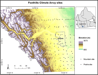
Figure 1 Foothills Climate Array study area. Crosses indicate mountain sites and dots are prairie sites. The City of Calgary municipal boundary is shown as a black outline. Sites within the boundary are classified as urban sites.

The main objective with the FCA was to understand and quantify spatial patterns of temperature as a function of elevation, topographic characteristics, surface type, and weather systems in this region. This includes conventional air temperature lapse rates (the change in minimum, maximum, and mean daily temperature with elevation) and their daily and geographic variability, but also other coherent patterns of temperature variance, to inform interpolation and downscaling models of temperature as a function of terrain and weather conditions. The FCA covers a large range of remote environments, with a high spatial density and 5 years of relatively complete data, spanning an elevation range of 890 to 2880 m. We are not aware of other mesonet arrays with this kind of spatial and temporal coverage in a mountain environment.

Here we present this unique multiyear temperature dataset, to support the public availability of this data and illustrate its relevance for environmental modelling and temperature downscaling. We describe the quality control and processing methods used to clean and filter the data, assess its accuracy, and present the distribution of daily temperature lapse rates in the region as a function of month and season. These lapse rate results can improve hydrological, ecological, or glaciological modelling applications in the region, where there is a need for distributed temperature estimates based on climate models or low-elevation reference stations.

2 Study region, design, and instrumentation

The FCA study area extends from the continental divide of the Rocky Mountains in the west to the relatively flat prairie farmlands about 50 km east of the city of Calgary, Alberta, centred on approximately 51^∘ N and 114.5^∘ W (Fig. 1). The Rocky Mountains, with altitudes up to 3500 m, straddle the border between British Columbia and Alberta in this region with a northwest-to-southeast alignment. The Bow River is a major river basin in the study area, cutting a southeast path through the mountains before turning east and exiting the mountains east of Canmore, Alberta. In the mountains, the floor of the Bow Valley has an altitude between 1300 and 1600 m, with peaks rising more than 1000 m on either side. There are also numerous alpine lakes and low-order creeks and tributaries of the Bow River that drain the steep mountain valleys.

Table 1 The number of sites having different elevation, slope, aspect, and land surface types.

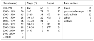
The upper slopes of the mountains are above the treeline and consist of rock and rubble, with sparse vegetation (see Table 1). Coniferous forest and alpine meadows occur below the treeline. The foothills are comprised of lower-elevation rolling hills, with coniferous and aspen forests interspersed with grassy meadows. The prairies are mostly shrub, grassland, and cultivated cropland, with farming the dominant land use. Sites are classified as mountain or prairie based on their elevation and terrain variability surrounding the site. Prairie sites are generally situated below 1250 m with little terrain variability. A total of nine sites are situated within the Calgary municipal boundary. Elevations drop to below 900 m at the eastern edge of the survey. Thus the area and site locations comprise a wide range of elevation, topography, and surface types, including grassland, cultivated farmland, urban, forest, shrub, meadow, and bare rock.

Each FCA installation consisted of rainfall, temperature, and relative humidity data-logging sensors mounted on a pole that was either pounded into the ground or supported with a cairn. Rainfall was recorded using HOBO RG2 tipping bucket rain gauges manufactured by Onset Computer Corporation. Temperature and relative humidity (RH) were recorded at 1 h intervals, with instantaneous measurements taken at the top of the hour, using SP-2000 temperature-relative humidity data loggers manufactured by Veriteq Instruments Inc¹. Daily mean temperatures are calculated as the arithmetic mean of hourly values. The data loggers were mounted inside radiation shields manufactured by Onset Scientific Ltd to protect the loggers from direct sunlight and allow air circulation. The manufacturer-reported accuracy for the sensors is ±0.25 ^∘C between −25 and +70 ^∘C, with a resolution of 0.02 ^∘C at +25 ^∘C. Where possible, temperature and RH were recorded at a height of 1.5 m above the ground. At sites in areas of significant snow accumulation (commonly at elevations above 2000 m), pole extensions were added to help keep the sensors above the winter snowpack and instrument heights were between 2 and 3 m.

Between 200 and 230 stations were in operation during the main recording period from July 2005 to June 2010. Site locations sampled the varying topography and land surfaces of the area, with an attempt to establish sites on a grid that would lead to a representative sampling of the landscape. Logistical realities meant that the FCA realization was not a perfectly regular grid. The local farming and ranching communities were co-operative, but permission to establish FCA sites on private land in the eastern part of the domain was not always granted, leading to gaps and irregularities. There are also numerous irregularities and gaps in coverage for the mountain sites, as some locations on the grid were inaccessible. Nonetheless, the sites effectively capture a range of elevations, slopes, aspects, and surface types (Table 1) and are statistically representative of the terrain in the region (Cullen and Marshall, 2011).

Given the remote environment, the FCA design criteria necessitated portable data-logging sensors that could be left in place for many years. We included sites that could be reached within a day's travel on foot or on bike (or commonly a combination of the two), and most of the mountain sites involved an off-trail approach from the nearest trail or road. It required about 160 person-days per year (80 days for a team of two) to complete the annual rounds. The infrequent site visits and sometimes hostile conditions (e.g., high winds, tree-fall, avalanches, flooding, vandalism, snow burial, wildlife interference) led to some challenges with data quality and missing data. The next section discusses data-processing and quality control procedures in detail.

The FCA installation began in spring 2004 and was completed in summer 2005. Data recording continued until autumn 2010, when all of the stations were taken down except for line 4, an east–west transect through the city of Calgary. Prairie sites were more accessible and were visited twice annually for site maintenance and data downloads, during the spring and autumn field seasons. Mountain sites were only visited once per year. Site maintenance included data collection, battery replacement, exchange of data-loggers as needed, instrument cleaning, and basic maintenance as required (e.g., reinstalled fallen or leaning instruments). The rain gauges, radiation shields, and sensors become dirty over time through exposure to dust, pollen, insects, and forest detritus (e.g., pine needles). Field notes and photographs were taken to document the physical location and condition of the sites during each visit.

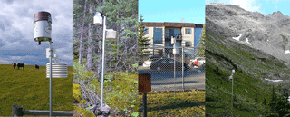
Sites do not conform to World Meteorological Organization (WMO) standards, which specify that climate recording sites should be level, away from vegetation and buildings, and not in areas of variable topography (WMO, 2008). This prescription is not consistent with the purpose of the study, which is to examine topographic and surface environmental influences on weather. In fact, it was part of the project design to sample different slopes, aspects, and degrees of forest closure, to quantify deviances from flat, open control settings. This contributes to the complex patterns of spatial temperature variability that we recorded, but in a manner that is realistic with respect to landscape-scale temperature modelling. Examples of site locations are shown in Fig. 2.

Figure 2 Site location examples: prairie, forest, urban, and mountain.

3 Sensor accuracy and quality control

3.1 Instrument calibration

Instruments were tested at the University of Calgary weather research station (WRS) before being set up in the field, and on an ongoing basis during the study to assess systematic bias or drift of the sensors. These tests were to determine whether it was necessary to apply bias or drift corrections to any sensors. Calibration tests consisted of sensors set up at the WRS and recording instantaneous temperature at 1, 2, or 5 min intervals for 1- to 2-week periods. Data were aggregated to hourly intervals and compared with aggregated hourly temperature measurements at the WRS reference station, which uses a Campbell Scientific HMP35CF sensor mounted in a ventilated, Gill Model 41004-5 12 plate radiation shield and records data at 1 min intervals. We used more frequent sampling which was then aggregated, in order to reduce the impact of once-off erratic readings which may have an undue influence during the short testing period.

Table 2 Test result statistics by year showing the total number of tests performed, the average difference between the hourly logger and WRS temperatures for all hours 00:00 to 24:00 MST, between 10:00 and 16:00 MST, and 00:00 and 06:00 MST.

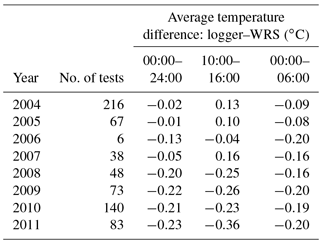
Average hourly differences were calculated for all sensors for all hours in a day (24 h), for hours between 00:00 and 06:00 MST (night), and between 10:00 and 16:00 MST (day). During the test period, if no absolute value of the hourly temperature difference between logger and WRS exceeded 3 ^∘C, a test was considered “good” and no further investigation of sensor performance was required. This was the result for 94 % of calibration runs. Average differences by year are shown in Table 2. The average difference between the Veriteq loggers and WRS is −0.1 ^∘C.

To more closely represent the actual data recording methodology, a similar analysis was performed whereby instantaneous measurements were extracted for each sensor and compared with corresponding WRS values. From the instantaneous measurements, daily minimum, maximum, and mean temperatures were extracted for each sensor and compared with WRS temperatures. The average differences between the Veriteq loggers and WRS are −0.26, −0.17, and −0.16 ^∘C for daily maximum, mean, and minimum temperatures, respectively. The average daily mean difference using instantaneous measurements was −0.2 ^∘C, compared with −0.1 ^∘C using aggregated hourly measurements.

Calibration tests after 2007 show more negative offsets relative to the earlier WRS values, possibly due to more tests being conducted during winter, where there may be less daytime heating effect or an overnight cooling effect in the naturally ventilated sensors. However, there was no apparent significant drift for individual sensors, nor did any sensors show consistent bias. Therefore, no corrections were applied.

Daytime heating can be an issue in naturally ventilated radiation shields, with a potential warm bias under calm, sunny conditions (Nakamura and Mahrt, 2005). Temperature sensors and shields have different associated errors, depending on the design of the shield, the type of sensor, and environmental conditions. The design of the shield should ensure that the air within the shield is at the same temperature as the surrounding air (WMO, 2008). Shields may rely on natural ventilation from prevailing winds or may be artificially ventilated using a fan.

Studies have investigated the magnitude of temperature differences for naturally vs. artificially ventilated sensors under different wind and solar radiation conditions (e.g., Georges and Kaser, 2002; Huwald et al., 2009). Daytime temperature differences are the greatest, due to solar heating, and can be problematic at wind speeds less than 1 m s⁻¹. This heating effect may be from direct radiative heating of the sensor or indirect heating of the shield, which then heats the air inside the shelter. We performed an experiment at the University of Calgary WRS from October 2012 to September 2013 to quantify the effect of using naturally ventilated sensors, as used in the FCA study, compared to a mechanically ventilated sensor used at the WRS. The Veriteq loggers were set to record instantaneous temperature at 5 min intervals, and hourly averages were calculated.

Table 3 The average hourly temperature difference (^∘C) between Veriteq loggers and the WRS temperature sensor at different wind speeds and incoming shortwave radiation values.

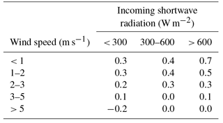
For this set of loggers, the average difference between hourly average logger and WRS temperatures was 0.1 ^∘C for the test period. Differences averaged for the whole year for the combined wind speed and incoming shortwave radiation categories are shown in Table 3. The maximum difference of 0.7 ^∘C occurs at high solar radiation (greater than 600 W m⁻²) and winds speeds less than 1 m s⁻¹. For high wind speeds and low solar radiation, the average difference is −0.2 ^∘C. Results in Table 3 are systematic and point to a relatively simple correction if hourly shortwave radiation and wind data are available. These are not available at the FCA sites, so this is a source of error that we must tolerate. However, the mean error in hourly temperature associated with the worst-case conditions is +0.7 ^∘C, and the daily average errors associated with naturally ventilated sensors are much less (solar radiation is less than 600 W m⁻² for most of the day, and throughout the winter). This source of error is likely insignificant for daily mean and minimum (overnight) temperatures, but it might affect maximum temperature measurements in sheltered locations. Sheltered sites may experience additional warming relative to exposed locations due to reduced ventilation, particularly in the summer months, but differences are expected to seldom exceed 1 ^∘C.

In the 6 % of calibration tests with suspect logger performance, the logger was flagged for further examination and field records for these loggers were manually inspected. Calibration experiments exhibited a common form of sensor failure associated with periods of heavy rainfall and sustained high humidity. Under these circumstances, some sensors experienced errant, short-term behaviour, typically recording temperatures that were too high for a period of hours to days, then returning to normal. Careful examination confirms that values before and after the observed aberrations are reliable, so we retain these sensors, but quality control measures described below are designed in part to identify this behaviour. The sensors are adequately sheltered, such that rainfall itself (liquid water) is not likely the problem; rather, we suspect that water vapour diffuses into the data loggers and internal condensation can compromise the circuit board, until such time as humidity drops and the sensor dries out.

3.2 Quality control

Assessment of data quality prior to data analysis is an essential step to ensure that only valid data are used. While sensors generally functioned well, periodically they malfunctioned or were damaged in the field, resulting in unreliable data. One challenge in identifying questionable data is to differentiate between extreme events and actual compromised data. Wade (1987) identified four general sources of measurement error, namely: instrument failure, drift, bias, and random error. Calibration tests identified that loggers do not show significant bias or drift, so these were not corrected for. Instrument failure is readily identifiable as missing data or unrealistic values. Random errors are more difficult to identify. We introduced a multi-step quality control/quality assurance (QC/QA) procedure for objective detection of errors.

Durre et al. (2010) detail comprehensive automated quality assurance procedures for daily meteorological measurements, as are being applied operationally in the Global Historical Climatology Network (GHCN). Quality control procedures are designed to identify as many errors as possible with few false positives (that is, valid data flagged as unreliable data). Tests used in the procedure include the following: (i) physically reasonable bounds; (ii) internal consistency – the daily value should be within statistical bounds for that day in the year; (iii) external consistency – the value should lie within reasonable limits of surrounding stations; (iv) multiple duplicate or repetitive values; (v) unusually large changes in daily minimum and maximum values. We use similar tests in this study.

Quality control procedures for the FCA data include a sequence of automated (A) and manual (M) data checks applied to an entire file, hourly, daily, or monthly data, and run in the order shown below.

• Field checks (M – entire file)

• Time shifts (M – hourly)

• Spikes (A – hourly)

• Snow burial (A/M – monthly)

• Neighbourhood consistency (A/M – daily)

• Review questionable loggers based on field notes and calibration tests (M – daily/hourly)

• Final review (M – daily/hourly)

3.2.1 Field checks

During the download process, each logger's data was compared with one or more near neighbours. Downloads were characterized as “good”, “some bad”, or “bad” using this comparison. Where a download was characterized as bad, the entire file was excluded. Files characterized as “some bad” were included and sections readily identified as erroneous based on a visual review were deleted.

3.2.2 Time shifts

The loggers adopt the start and end time from the computer doing the setup and download. The Spectrum v3.7c software uses the computer download time to assign a time to each measurement. Multiple machines were used for field downloads and at times the clocks were set to the wrong time zone, or alternated between daylight savings time (DST) and mountain standard time (MST). Times were commonly out by several minutes. In addition, on occasion some loggers malfunctioned and missed recording data for hours or days at a time, as seen in comparisons with neighbours. This was noted in the field notes.

The data loggers are able to store approximately 18 months of data recorded at 1 h intervals. If the time between site visits was too long, or a logger was inadvertently set to record at a shorter time interval, the memory filled up and no more data were recorded. By comparing multiple neighbours, and reviewing field notes which included the actual download time and whether time was DST or MST, files with time shifts and missing data were identified. Once the data were loaded into the database, the necessary time shifts were applied. Where possible, periods of missing data were identified and measurement times adjusted to align data with neighbours.

3.2.3 Spikes

A directional step test used by Hall et al. (2008) identifies consecutive measurements exceeding a user-defined limit. Limits vary by location (climate region), measurement interval, and direction (rise or fall). Temperature changes of up to 9 ^∘C in 5 min have been observed in the Oklahoma mesonet. Due to such events, Graybeal et al. (2004) found step tests were capturing actual frontal events, whereas data problems were predominantly 1 h spikes rather than step changes in the data. In southern Alberta, chinook winds and cold fronts cause both large rises and falls in hourly temperature measures, but these conditions usually persist after the step change. Temperature swings of greater than 30 ^∘C in a day have been observed at the onset of chinook winds (Nkemdirim, 1988).

A review of FCA data identified by step tests indicates spikes, either up or down, lasting 1 h or more can be real errors. A brief spike may not influence daily mean values enough to be identified as unusual relative to neighbours (cf. neighbourhood consistency check described later), but spikes lasting 4 h or more will. Therefore, a spike test to identify spikes lasting from 1–3 h was applied to FCA data. A spike was defined as a value exceeding subsequent or previous measures up to 3 h apart by 5 ^∘C, either up or down.

3.2.4 Snow burial

Some of the high mountain sites were prone to burial by snow during late winter. Snow burial is apparent through a small diurnal temperature range. For the snow burial test, we flag entire months where at least 25 days have a diurnal range of less than 3 ^∘C. Days on either side of the flagged months are examined for snow burial signal and manually flagged. Commonly, snow burial was identified during field checks, and blocks of data were deleted based on a visual comparison with neighbouring sites.

3.2.5 Neighbourhood consistency

Neighbourhood consistency checks are used to identify unusual values at a site relative to neighbouring stations. The method, threshold values, and number of stations used depend on station density, topography of the area, and the weather variable being checked. In all cases, estimated values calculated from neighbouring sites are compared to observed values and large deviations are flagged as potential errors.

Shafer et al. (2000) use a weighted average of neighbouring stations to calculate a value for the station being checked, with differences exceeding 3 standard deviations flagged as suspicious. In mountain regions, Lanzante (1996) suggests using vertical neighbours (closest station with a similar elevation) as an alternative to horizontal proximity.

As a means of identifying the most appropriate neighbours, we specified two spatial neighbourhoods for the FCA data. A horizontal-proximity neighbourhood was defined using all sites within a 25 km radius of a site (50 km for sites at the edge of the survey), and a vertical neighbourhood was defined using sites in 200 m elevation bands, e.g., 1400 to 1600 m, 1600 to 1800 m. All sites above 2200 m are grouped together; therefore, this group includes the two high-elevation sites above 2800 m, with the remainder of the sites being less than 2500 m. In all cases, groups consist of at least 10 sites.

The spatial proximity test accounts for local variability and the elevation band accounts for elevation consistency. The test examines daily minimum, maximum, and mean values for each site compared to the average and standard deviations calculated from all sites within elevation and horizontal-proximity neighbourhoods. In calculating the neighbourhood average and standard deviation for each day, the site(s) with the lowest and highest values within the group are excluded, as are all site-days flagged as errors in previous quality control tests.

As an initial screening procedure, site-days are flagged as suspect if their daily minimum, maximum, or mean value differs from both horizontal-proximity and elevation-band neighbourhood means by more than 5 standard deviations. All suspect site-days are then manually reviewed and flagged as either natural variability or unreliable data. For sites identified as unreliable data, manual review generally indicated erratic sensor performance, and the threshold for questionable data was reduced to 3 standard deviations. All days for these sites are flagged as unreliable where any of the daily minimum, maximum, or mean exceeds the group mean values by 3 or more standard deviations.

3.2.6 Manual review of field notes

Field notes indicated any obvious issues with the site itself or unusual data. For instance, stations were sometimes found to have fallen or been knocked over. In this situation, station data were examined in relation to elevation and proximity neighbours as in the neighbour consistency check, to identify the time at which the station fell over. Sensors at ground level record too-high maxima and too-low minima during summer, and would typically become snow-buried during the winter. All data from the time of station compromise were removed.

3.2.7 Final review

Apart from entire files or obvious bad data blocks excluded from the compiled file, data are flagged as bad rather than being deleted. A different flag is assigned for each quality control test failure. The final review looks at groups of data with flags turned on or off to verify that tests have correctly identified errant data, and no suspect data remains. Any further bad data identified in this final review, most commonly seen in days on either side of failed test days or very few days remaining in a month, are flagged.

As the topography of the FCA and the climate of southwestern Alberta show high variability, quality control checks were applied leniently in order to retain interesting data; therefore, some questionable data may be retained as well. On average, 91 % of data were good and 9 % of data were flagged as unreliable and excluded from the analysis. Missing data are distributed randomly in the study area, with missing or suspect data affecting 70 % of the sites.

4 Gap-filling of missing data and monthly lapse rates

While overall data coverage is excellent, given the remote nature of the FCA and the infrequent site visits, missing data do compromise the utility of the dataset, e.g., in determination of monthly or annual means. Stooksbury et al. (1999) show that 3-day data gaps can result in errors of ±1 ^∘C in the calculation of monthly means, with larger errors during winter and in continental interior locations. Missing or erroneous data can also cause poor performance such as spatial or temporal discontinuities in interpolation or modelling of temperature surfaces. We therefore introduce gap-filling measures for the 9 % of the data that is missing, to make for straightforward and reliable application of this dataset.

Approaches to gap-filling depend on the environment and the neighbourhood of stations that are available for modelling of missing data. Nkemdirim (1996) created monthly regression equations using closely correlated stations to recreate daily minimum and maximum temperatures in southern Alberta. Eischeid and Pasteris (2000) used between one and four most closely correlated neighbouring stations to estimate daily minimum and maximum temperatures for the western United States, using a version of the general linear least squares regression estimation with least absolute deviations criteria. Both studies calculated correlations on a monthly basis. However, Courault and Monestiez (1999) note that station correlations vary with wind direction and topographic location, indicating that the most correlated station may vary during any month.

We tested gap-filling methods using the most closely correlated stations, calculated by month and by weather type for each of daily mean, minimum, and maximum temperatures. The latter requires a classification system for regional weather systems, which we describe briefly below. Days are grouped by month and by weather type. For each group, correlation coefficients are calculated between all possible station pairs for each of daily mean, minimum, and maximum temperatures. For each station, temperature measure, and group (month or weather type), neighbour stations are ordered by correlation with the target station from high to low and the most highly correlated neighbour station for each target station and group is identified. Station temperatures are highly correlated, but the coefficients and most highly correlated station do vary by month and weather type. A regression–prediction equation is generated for each station–neighbour pair for each group. Missing daily temperature measures are calculated using the prediction equation for the group to which the day belongs (month and weather type), and, for each station, the most highly correlated neighbour station with available data is used to calculate the missing temperature. The next two sections briefly describe the weather classification system and the accuracy of the gap-filling methods. Readers are referred to Wood (2017) for further details.

Table 4 Selected qualitative surface meteorological characteristics associated with different weather types in southern Alberta.

4.1 Weather system classification

We classify daily weather type based on a discriminant function analysis (DFA), seeded with the surface characteristics of the primary weather patterns that occur in our study region (Table 4). Daily weather conditions are characterized from the long-term data available at the Meteorological Service of Canada station at Calgary International Airport (Environment Canada, 2015). We explored a wide array of daily weather variables, including temperature, pressure, humidity, wind speed, and 500 hPa geopotential height, along with measures of the 24 h trends and variance in these variables (Wood, 2017). Mean daily conditions for the period 1970–2010 are calculated using an 11-day moving window. Daily weather anomalies are then calculated from these mean values in order to remove the influence of seasonal cycles and provide a year-round classification system (Wood, 2017).

The control groups for the DFA weather types are based on manually classified daily weather conditions from October 2013 to September 2014. DFA provides a multivariate method to characterize a given weather type in our region, based on daily weather conditions. There is an implicit assumption that a given weather type, e.g., a chinook or an anticyclonic ridge over the region, will have similar weather anomalies throughout the year, and from one year to the next. The DFA classification can then be applied across time. The period used for creating the discriminant functions does not overlap with the FCA data collection period, but these periods are only a few years apart, so mean climate conditions are not expected to have changed much and the discriminant functions should still be appropriate. The DFA method also requires that the dominant weather-system types are all represented in the calibration period (2013–2014), as per our seed groups. Exotic weather types during the FCA period will not be captured through this approach, but our interest here is to characterize the most common regional weather systems. The identified weather classes include the following: (i) cold, dry (i.e., continental polar) air masses (CD); (ii) chinook conditions (Ch); (iii) cool, wet (cyclonic) weather systems (CW); (iv) warm, high-pressure conditions (Ht); (v) cold-front transition days (Tr); and (vi) normal conditions (Nl), which are defined as days with surface weather characteristics within 1 standard deviation of their long-term mean value. Selected characteristics of these weather types are listed in Table 4. Wood (2017) provides additional details.

The accuracy for the final DFA model is 81 % using jackknife cross-validation, where each day is left out in turn; prediction functions are calculated with the remaining data, and these functions are used to predict the omitted day. The CD and Nl types are consistently well-predicted, with accuracies between 80 and 90 %, while the remaining types vary from 50 to 90 % accuracy, with transition days proving to be the most difficult to capture.

The spatial characteristics of weather systems were found to vary seasonally, so weather types were further divided into seasonal subgroups. Three seasons were defined as follows: winter (November to February), summer (May to August), and autumn–spring (September, October, March, April). As the normal weather type (Nl) comprises more than 50 % of days, and correlations and topographic influences show an annual cycle, correlations were also calculated for Nl days grouped by month.

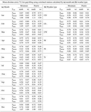
Table 5 Estimated gap-filling errors shown as mean absolute temperature errors (^∘C) calculated as the difference between actual temperature and temperature estimated using the most highly correlated station by month (mnth) and weather type (wt), shown for each (a) month and (b) weather type for prairie and mountain sites.

4.2 Accuracy of the gap-filling models

Errors associated with the gap-filling models are shown in Table 5. Mean absolute errors by month and weather type are shown for minimum (T_min), maximum (T_max), and mean daily (T_mean) temperatures. Values are further divided into mountain and prairie subsets of the data. Weather-type estimates are better than those based on monthly correlations, with T_mean having the lowest errors, followed by T_max and T_min. Errors for all temperature measures are larger in the cold months, November to February. Although there is still a lot of inherent variability within weather types, seasonal-weather-type correlations improve estimates by ∼ 7 % over monthly correlations. Error reductions based on weather type are most significant for cold-front transition, cool–wet, and chinook days.

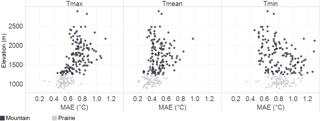
Missing temperature data in the FCA are gap-filled using regression equations generated using the most closely correlated station for each site, where correlations are calculated by seasonal weather type. The accuracy of the gap-filling equations was assessed using jackknife cross-validation, where daily temperature measures for each site and day with data are estimated from temperatures from the most closely correlated station using regression equations. Mean absolute errors based on seasonal-weather-type correlations range from 0.40 ^∘C (T_mean in the prairies) to 0.84 ^∘C (T_min in the prairies). Of site-day errors for all methods, 90, 95, and 98 % are less than 2 ^∘C for T_min, T_max, and T_mean, respectively. Figure 3 plots mean site error estimates vs. elevation. Errors in T_max and T_mean increase with elevation and are lowest for the prairie sites. Errors for T_min show a weaker negative relationship with elevation.

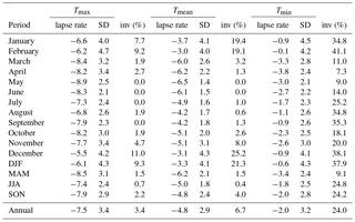
Table 6 Mean and standard deviation (SD) of temperature lapse rates (^∘C km⁻¹) and inversion frequency (%) for daily minimum, maximum, and mean temperature, by month and season.

Figure 3 Estimated gap-filling errors shown as mean absolute error (MAE) for each site as a function of elevation. Errors are calculated as the differences between the actual temperature and the temperature estimated from the most closely correlated station.

4.3 Monthly lapse rates in the foothills region

Temperature lapse rates are commonly required in ecological and hydrological models and for downscaling of scenarios from climate models. The FCA data provide a 5-year record of daily temperature lapse rates, calculated from regressions of T_min, T_max, and T_mean vs. elevation for the FCA mountain data. Mean values and standard deviations are summarized in Table 6. Monthly values are based on the mean of individual days; over 5 years, this gives N ≈ 150 for each month in Table 6. Inversion frequency is also reported for each period and temperature measure, calculated from the percentage of days with positive lapse rates. The strength of the linear regression (R² value) for monthly lapse rates gives an indication of how well a linear lapse rate represents the data, and this varies systematically by season and by temperature measure. Mean values vary from 0.5 to 0.8 for T_max, 0.4 to 0.8 for T_mean, and 0.15 to 0.4 for T_min and are weakest during the winter months. R² is also weak during summer months for T_min.

There are significant differences in lapse rate between minimum, mean, and maximum temperatures and the monthly inversion frequencies for each. Maximum temperature has the steepest lapse rates in all months and is the least prone to inversions with altitude. Monthly values range from −5.5 to −8.9 ^∘C km⁻¹ and are steepest in the spring and autumn. On average, maximum temperature inversions occur only 1.5 % of the time outside of the winter months (i.e., from March through November), and 9.3 % of the time from December through February (DJF). Winter inversions are common in this region in association with cold, continental polar air masses (Cullen and Marshall, 2011), and these air mass inversions are sometimes strong enough to persist through the day, affecting the maximum temperatures. Under these conditions, comparatively warm, westerly air commonly overrides the shallow, cold air mass that is in place, supporting the inversion structure.

Mean and minimum temperatures show similar seasonal structure to maximum temperatures, with the steepest and shallowest values in spring and winter, respectively. Inversion frequency and lapse rate variability are much greater in the winter season, and are lowest in the summer. Monthly lapse rates for mean temperature vary from −3.0 to −6.5 ^∘C km⁻¹, with an annual mean of −4.8 ^∘C km⁻¹. Regional-scale inversions occur on 21 % of days in the winter season, but are relatively rare in the spring, summer, and autumn (2 % of days). Minimum temperature lapse rates are shallower, varying from −0.1 to −3.8 ^∘C km⁻¹, with an annual mean of −2.0 ^∘C km⁻¹. This is a large departure from free-air lapse rates, and is driven by the overnight development of cold-air drainage and pooling at lower elevations, as well as the prevalence of cold, shallow air masses in the study region, particularly in the winter season. Minimum temperature inversions are observed on 38 % of days in the winter months and 24 % of days annually and are common in all seasons.

5 Data availability

Data described are available on the PANGAEA repository https://doi.org/10.1594/PANGAEA.880611 (Wood et al., 2017). Minimum, maximum, and mean daily temperature data are available as well as site attributes – latitude, longitude, elevation, land surface type, site type, sensor height above ground, and whether the temperature values are measured or estimated.

6 Summary

Data gathered within the Foothills Climate Array offer a unique collection of high-density, multiyear observations in complicated mountain terrain. These data provide a detailed three-dimensional view of the near-surface temperature structure and its temporal variability as a function of season and weather type.

The Veriteq temperature instruments used in this study performed exceptionally well, with high accuracy and no drift over time. Multistage quality control procedures were successful in identifying and removing questionable data. In total, 9 % of data collected at the ∼ 230 sites between 2005 and 2010 are missing or unreliable. Missing and unreliable data are distributed randomly in the study area. While the dense station network provides some redundancy and the percentage of missing data is not high, gap-filling to create a complete dataset has benefits for applications requiring monthly means or for creating interpolated temperature surfaces. We therefore gap-filled the data that is presented here, with a flag to denote that these data have been estimated.

Daily temperature lapse rates in the southwestern Alberta foothills show a strong seasonal cycle, with shallower values and greater variability in the winter months. Lapse rates of maximum temperature are steeper and are similar to free-air lapse rate values (e.g., −7.5 ^∘C km⁻¹) that are commonly used in temperature downscaling or extrapolation in mountainous terrain, but lapse rates of mean and minimum temperature are much shallower, with mean annual values of −4.8 and −2.0 ^∘C km⁻¹, respectively. Minimum temperature inversions are frequent year-round, and are present on 38 % of days in the winter months.

The temperature and lapse rate structure reported here are specific to our region, but the general behaviour of temperature variations over the terrain and the observation of systematic daily and seasonal lapse rate variability are expected to be relevant to all mountain regions. In mid-latitude regions like our study area, there is additional complexity due to air mass and frontal interactions, and their interaction with the terrain. These effects will be examined in more detail elsewhere, through consideration of daily weather types and their influence on regional temperature patterns and lapse rates.