Environmental conditions of a salt-marsh biodiversity experiment on the island of Spiekeroog (Germany)

Field experiments investigating biodiversity and ecosystem functioning require the observation of abiotic parameters, especially when carried out in the intertidal zone. An experiment for biodiversity–ecosystem functioning was set up in the intertidal zone of the back-barrier salt marsh of Spiekeroog Island in the German Bight. Here, we report the accompanying instrumentation, maintenance, data acquisition, data handling and data quality control as well as monitoring results observed over a continuous period from September 2014 to April 2017. Time series of abiotic conditions were measured at several sites in the vicinity of newly built experimental salt-marsh islands on the tidal flat. Meteorological measurements were conducted from a weather station (WS, https://doi.org/10.1594/PANGAEA.870988), oceanographic conditions were sampled through a bottom-mounted recording current meter (RCM, https://doi.org/10.1594/PANGAEA.877265) and a bottom-mounted tide and wave recorder (TWR, https://doi.org/10.1594/PANGAEA.877258). Tide data are essential in calculating flooding duration and flooding frequency with respect to different salt-marsh elevation zones. Data loggers (DL) for measuring the water level (DL-W, https://doi.org/10.1594/PANGAEA.877267), temperature (DL-T, https://doi.org/10.1594/PANGAEA.877257), light intensity (DL-L, https://doi.org/10.1594/PANGAEA.877256) and conductivity (DL-C, https://doi.org/10.1594/PANGAEA.877266) were deployed at different elevational zones on the experimental islands and the investigated salt-marsh plots. A data availability of 80 % for 17 out of 23 sensors was achieved. Results showed the influence of seasonal and tidal dynamics on the experimental islands. Nearby salt-marsh plots exhibited some differences, e.g., in temperature dynamics. Thus, a consistent, multi-parameter, long-term dataset is available as a basis for further biodiversity and ecosystem functioning studies.

1 Introduction

Biodiversity is changing at an unprecedentedly high rate (Mace et al., 2005), reflecting the anthropogenic alteration of Earth's ecosystems (Rockström et al., 2009). As a consequence, research on biodiversity–ecosystem function (BEF) relationships has become a major facet of ecology and evolutionary biology (Balvanera et al., 2006; Cardinale et al., 2006; Hillebrand and Matthiessen, 2009; Cadotte et al., 2008; Gravel et al., 2011). Research on BEF has been dominated by experimental studies manipulating the number of species in a trophic group (Hillebrand and Matthiessen, 2009). However, the change in the number of species is not the predominant pattern in biodiversity change, which more frequently comprises altered dominances and species turnover (Hillebrand et al., 2017). Moreover, the mechanisms involved in altering species composition, i.e., immigration and extinction, are usually experimentally prohibited in most BEF studies, e.g., via weeding. On the other hand, there have been recent advances in understanding the interaction between regional community assembly, local dynamics and the biodiversity-functioning aspects (Hodapp et al., 2016; Leibold et al., 2017) that should be incorporated in BEF experiments.

The intertidal zone represents an interface between terrestrial and marine processes and biodiversity. This area is sensitive to climate change and is heavily impacted by anthropogenic activities (Cooley and Doney, 2009; Ekstrom et al., 2015; Haigh et al., 2015; Mathis et al., 2015). Within the intertidal environment, salt marshes have increasingly gained attention in times of sea-level rise (Kirwan and Megonigal, 2013; Balke et al., 2016), but studies on meta-community dynamics remain scarce.

Based on this backdrop the project BEFmate “Biodiversity–Ecosystem Functioning across marine and terrestrial ecosystems” was conducted in March 2014–December 2017, aiming to quantify the dynamics of biodiversity and the associated functions of salt marsh and tidal flat ecosystems. For this purpose, a series of experimental islands were set up in September 2014 on the back-barrier tidal flat of Spiekeroog island in the German East Frisian Wadden Sea (Balke et al., 2017) and were mirrored by salt-marsh enclosed plots located within the nearby salt marsh. Here we report abiotic parameters observed from 23 sensors installed either near the experimental islands, within the island structures themselves or within the nearby salt marsh as well as meteorological data from a locally installed weather station. We describe the instrumentation, data handling and results observed over a period of 32 months starting from the middle of September 2014. We further discuss the data and results with respect to validity and potential limitations of the observational setup.

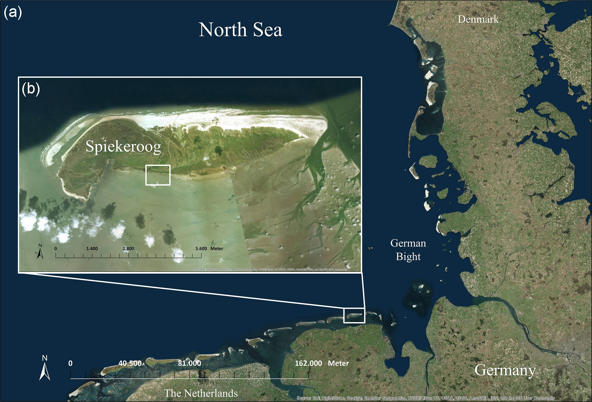
Figure 1 (a) Island of Spiekeroog located in the German Bight (North Sea). (b) The study site is located south of Spiekeroog (white box).

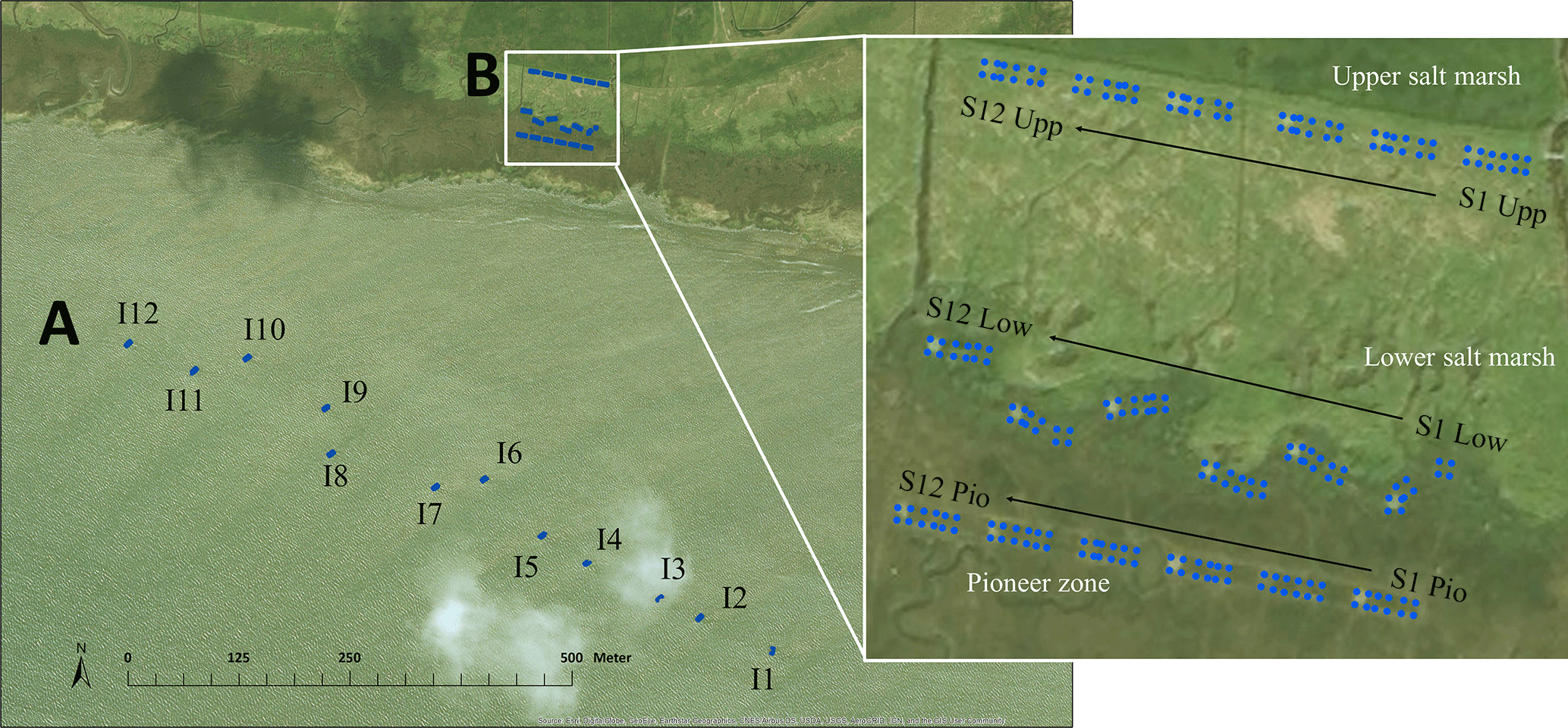
Figure 2 Experiment setup with (a) experimental islands in the back-barrier tidal flat and (b) salt-marsh control plots at different elevational zones in the salt marsh. Both, island and salt-marsh experimental plots are numbered from 1 to 12 from east to west.

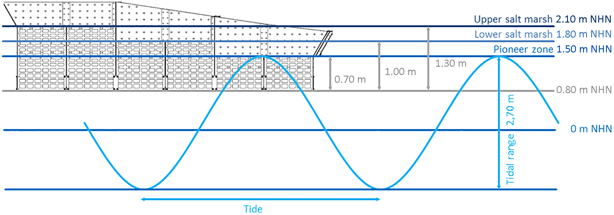
Figure 3 Scheme of an experimental island showing three elevational levels representing natural salt-marsh zones. The islands are built on an average of 0.8 m NHN (normal height null). The experimental islands' outer hull (galvanized steel) is patterned in the upper area to allow for a lateral water exchange. Lower area pattern is only meant to reduce weight and ease construction.

2 Materials and methods

2.1 Research area

The island of Spiekeroog is located in the southern North Sea (Fig. 1) and is part of the Wadden Sea, which has been renowned as an UNESCO world natural heritage site since 2012. Twelve experimental islands (I1–I12) were built in the back-barrier tidal flats at distances of 240 m (I12) to 460 m (I1) from the southern salt marsh of the island of Spiekeroog. The experimental islands were distributed unevenly over 810 m from east to west at an elevation of 0.8 m NHN (standard height zero), with a mean tidal range of 2.7 m (Fig. 2, numbered 1–12 from east to west). The islands were built in a northeast–southwest direction, with the lowest elevation at the northeastern end of the island. The actual sensor position on the islands was determined by the local bathymetry, since the experimental islands encompass three different elevation levels (Fig. 3) that consist of the reflecting pioneer zone (Pio; 1.5 m NHN), lower salt-marsh zone (Low; 1.8 m NHN) and upper salt-marsh zone (Upp; 2.1 m NHN) of natural salt marshes. Half of the experimental islands were filled with mudflat sediment and left bare, whereas half of them were additionally transplanted with sods from the lower salt-marsh zone of the natural adjacent salt marsh. Experimental islands represent a treatment of dispersal limitation, constraining community assembly on the islands. Additionally 12 equally treated salt-marsh enclosed plots (S 1–12) were created (Fig. 2) that reflect unlimited dispersal. In addition to experimental plots, six control plots (C) per salt-marsh elevation zone were marked but left natural to compare established communities with the community assembly on dispersedly limited island plots and unlimited salt-marsh plots. The experimental design and setup of the experimental islands are not subject of this work and are described in detail in Balke et al. (2017). Abiotic conditions were measured at several sites due to the involvement of wide selection of parameters. Details concerning the individual sensors, their location, data provided and the associated methods of data handling are provided in the following subsections. All positions, coordinates and elevations of sensors are indicated and provided in Table 1.

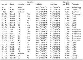
Table 1 Overview of all installed loggers at the experimental islands (I) and the salt-marsh enclosed plots (S) as well as the nearby installed sensors. WS: weather station, RCM: recording current meter, TWR: tide and wave recorder, DL: data logger.

2.2 Instrumentation and data processing

2.2.1 Weather station (WS)

Meteorological data were collected near the experimental setup (see Table 1), with a locally installed weather station located approximately 500 m north of the southern shoreline (53^∘45^′57.10${}^{\prime \prime }$ N, 007^∘43^′34.11${}^{\prime \prime }$ E). The system was installed at the end of a glass fibre pole at a height of 10 m. The weather station system used here was a ClimaSensor US 4.920x.00.00x that was pre-calibrated by the manufacturer (Adolf Thies GmbH & Co. KG, D-Göttingen). Data were recorded and saved within the Meteo-Online (V4.5.0.20253) software in a sampling interval of 1 min, with an averaging time of 10 s, and the date and time were given in UTC. The position, solar azimuth angle and solar elevation were derived from the internal GPS system. Ultrasonic propagation time measurements were used for the determination of wind speed and direction. Two sensors were integrated for measuring air temperature and relative humidity (precision combination sensor) as well as atmospheric pressure (micro-electro-mechanical system technology). For recording and calculating precipitation, the back-reflected signal of a Doppler radar was used. An additional four photo sensors were used for the identification of light direction and light intensity. The post-processing of collected data was done using MATLAB (R2012b). Further quality control was performed by (a) erasing negative readings and data covering maintenance activities and (b) removing the outliers, defined as data exhibiting changes of more than two standard deviations within one time step. As the weather station was not oriented directly towards north, a manual correction to the north had to be done afterwards for accurate wind direction values (+20^∘ from November 2014 to March 2016 and +10.1^∘ since October 2016).

2.2.2 Recording current meter (RCM)

A RCM9 LW recording current meter (AADI, Aanderaa, Bergen/Norway; RCM DCS 4220) with additional temperature (3621), conductivity (3919) and pressure (4017) probes was deployed for deriving hydrographic conditions (see Table 1). The device was bottom mounted through a buried H-anchor between islands 6 (I6) and 7 (I7) (53^∘45^′29.34${}^{\prime \prime }$ N, 007^∘43^′16.50${}^{\prime \prime }$ E), approximately 35 m southeast of island 7 and 50 m southwest of island 6 in a shallow tidal creek (0.71 m NHN). The position was derived from a portable DGPS system (Leica Differential-GPS, SR530). The acoustic sensor head was placed 0.4 m above the sediment at 1.2 m above the mean low-water height. As a consequence, the sensor head became dry during low tide, and data had to be examined and eliminated accordingly. The sensor was pre-calibrated by the manufacturer. Recorded data were internally logged on a memory card (DSU 2990 E), with a sampling interval of 10 min until the readout with the Data Reading Program DRP 5059 software. The sampling interval was chosen to resolve the tidal changes expected (dominant M2 lunar tide with 12.4 h period) while at the same time providing a minimum deployment time of 2 months between services to account for the environmental protection regulations in this area. The same sampling interval was applied to the other sensors in this setup, except for the weather station. Date and time was given in UTC. Post-processing was performed using MATLAB (R2012b) to remove low-tide data. Conductivity values were used as an indicator of low-tide periods. Data were erased when conductivity values fell below 25 mS cm⁻¹. Further quality control was applied as described in Sect. 2.2.1 for the weather station (WS).

2.2.3 Tide and wave recorder (TWR)

Local tide and wave conditions were recorded with a RBRduo TD|wave sensor (RBR Ltd., Ontario/Canada). The sensor was bottom mounted in a shallow tidal creek (0.71 m NHN) through a steel girder (buried 0.3 m deep in the sediment) next to the RCM 9 LW recording current meter between islands 6 and 7 (53^∘45^′29.34${}^{\prime \prime }$ N, 007^∘43^′16.50${}^{\prime \prime }$ E) (see Table 1). The sensor was positioned 10 cm above sediment surface, as was determined by using a portable differential GPS (Leica Differential-GPS, SR530). This resulted in the sensor falling dry during low tide and data had to be flagged accordingly. The sensor was pre-calibrated by the manufacturer and the sampling rate was 3 Hz with 1024 samples per burst at a sample interval of 10 min. Recorded data were internally logged until the readout with the Ruskin (V1.13.10) software and post-processed using MATLAB (R2012b). Date and time was given in UTC. For accurate depth calculations, raw pressure data were manually corrected for atmospheric pressure derived from the locally installed weather station. Low-tide data were not removed, but were easily identified through the manually calculated water depth data, where all depths <0.05 m represented low-tide data. Again, quality control was applied as described in Sect. 2.2.1 for the WS.

2.2.4 Data logger (DL)

Several data loggers were installed on the experimental islands as well as in the salt-marsh enclosed plots for the observation of groundwater level, temperature, light and salinity (see Table 1). In all cases the date and time is given in UTC and all post-processing was performed using MATLAB (R2012b). Quality control was applied as described in Sect. 2.2 for the weather station (WS).

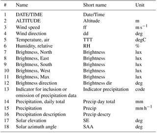
Table 2 Structure of the weather station (WS) datasets at PANGAEA.

To continuously observe the flooding and the groundwater levels on the experimental islands as well as in the salt marsh, pressure loggers were deployed in dip wells within the experimental setup at different elevational levels. Six HOBO^® U20L Water Level Logger (onset^® HOBO^® Data Loggers, Bourne, MA, USA; S/N 10685287, 10685288, 10685289, 10685290, 10685291, 10685292; Hobo-P) as well as a DEFI-D Miniature Pressure Recorder (S/N OA5K008; DEFI-D) were deployed. All water level loggers were pre-calibrated by the manufacturer. Recorded data were internal logged until the readout afield with the Hobo Underwater Shuttle (U-DTW-1) and the HOBOware Pro (V3.7.4) software respectively with the DEFI Series software (V1.02). For depth calculations, pressure data were manually corrected by atmospheric pressure. Accordingly, a HOBO^® U20L Water Level Logger was installed outside the dip wells at a higher elevation, attached on a steel pole at the upper zone of island 3. All loggers were initially calibrated to get the exact height inside the dip well. Data of one of the HOBO loggers had to be corrected with −0.082 m due to a wrong initial measurement. Further corrections were applied to the DEFI-D Logger, since a manual correction with atmospheric pressure was not possible. As the local maxima of other water level loggers were very similar, a mean value of other loggers was calculated to correct the DEFI-D logger values with +0.25 m.

Table 3 Structure of the recording current meter (RCM) datasets at PANGAEA.

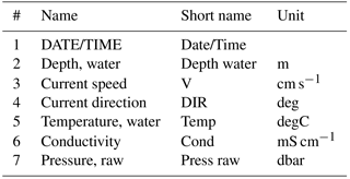
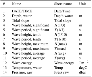
Table 4 Structure of the tide and wave recorder (TWR) datasets PANGAEA.

Temperature in the sediment surface layer (in approximately 0.05 m depth) was measured with six DEFI-T miniature temperature recorders (JFE Advantech Co., Ltd., Tokyo; DEFI-T). The manufacturer pre-calibrated temperature recorders and were installed on the experimental islands and in salt-marsh enclosed plots at different elevation levels. Recorded data were internally logged until the readout with the DEFI Series software (V1.02).

Light availability was measured with six locally installed light intensity loggers on the experimental islands as well as in the salt-marsh plots at different elevation levels. The DEFI-L Miniature Light Intensity Recorder (JFE Advantech Co., Ltd., Tokyo; DEFI-L) used here were pre-calibrated by the manufacturer. Recorded data were internally logged until the readout with the DEFI Series software (V1.02). Due to different calibrations for underwater or above-water applications, raw data were processed differently and merged depending on water levels. The processed pressure and depth data of the RBRduo TD|wave sensor were used to identify the flooding times and durations of the different elevations.

Table 5 Structure of the water level logger (DL-W) datasets at PANGAEA.

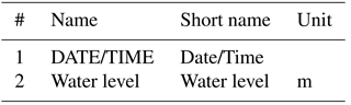
Table 6 Structure of the temperature logger (DL-T) datasets at PANGAEA.

Table 7 Structure of light logger (DL-L) datasets at PANGAEA.

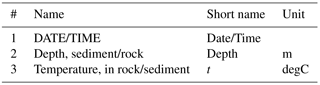
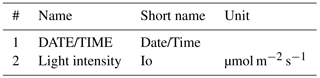
Table 8 Structure of conductivity logger (DL-C) datasets at PANGAEA.

Two HOBO conductivity loggers (Onset Computer Corporation, Bourne, MA, USA) were installed inside of dip wells on the experimental islands as well as in the salt-marsh enclosed plots at the pioneer zone. The conductivity logger used here was the HOBO U24 Conductivity Logger U24-002-C (S/N 10570000, 10599255). The conductivity loggers were pre-calibrated by the manufacturer. Recorded data were internally logged until the readout afield with the Hobo Underwater Shuttle (U-DTW-1) and in the following with the HOBOware Pro (V3.7.4) software. An automatic calculation of salinity was conducted within the software according to PSS-78 using the measured conductivity and temperature. Due to fluctuations in the groundwater level, conductivity loggers periodically became dry, especially in the beginning of the deployment. Data until October 2015 are therefore very scattered. The depth of conductivity loggers was thereupon adjusted to the bottom of the dip wells, assuring a constant coverage with water. Data from dry sensors was removed, using a salinity of 20 as a threshold value. As a reference, soil samples of all plots on the experimental islands and salt-marsh enclosed plots were sampled to analyze pore water salinity in laboratory (data not shown here). Comparative data of meteorological and hydrographic conditions for validation processes were taken from the nearby Time Series Station – Spiekeroog (TSS) at Otzumer Balje (Holinde et al., 2015; Baschek et al., 2017).

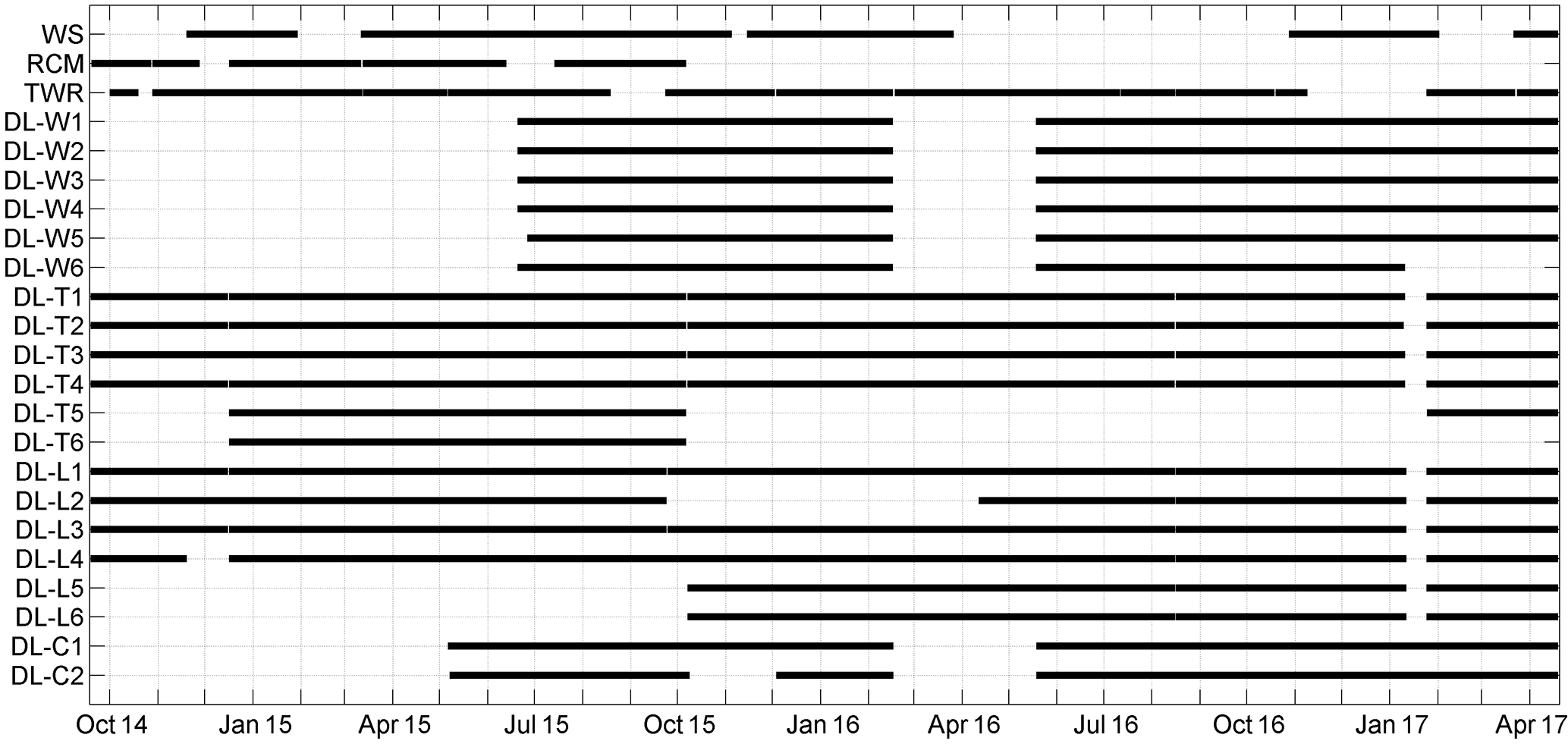
Figure 4 Available data shown in black bars for each sensor or logger type over the sampling period from 18 September 2014 to 18 April 2017.

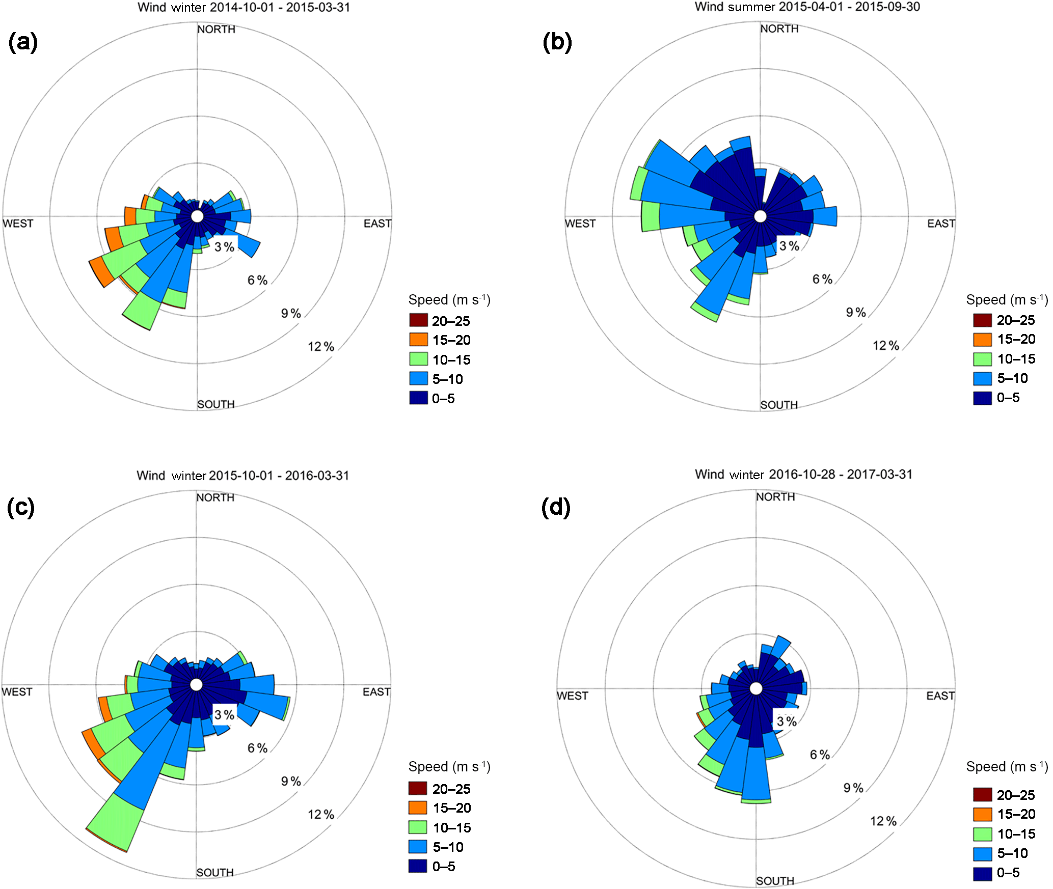
Figure 5 Local wind roses (wind speed and wind direction) for storm seasons (1 October–31 March) in 2014 and 2015 (a), 2015 and 2016 (c) and 2016 and 2017 (d) as well as for one summer season (1 April–30 September) in 2015 (b).

2.3 Data provenance, structure and availability

All datasets described herein are available at the World Data Center PANGAEA (https://www.pangaea.de/) when searching for “BEFmate” as identifier (Zielinski et al., 2017a–g). Due to extensive datasets as well as individual questions of potential users, a collection (parent) for each sensor (type) was created. Each parent serves as a basis where data are divided into monthly sections enabling an easy selection of required time periods. The raw data and MATLAB routines applied in the curation process are available on request.

2.3.1 Weather station (WS)

Data of meteorological observations are available at PANGAEA from November 2014 to April 2017 (https://doi.org/10.1594/PANGAEA.870988). Gaps in the dataset resulted from a malfunction of the pressure sensor and an adjacent maintenance and re-calibration by the manufacturer. The structure of dataset is shown in Table 2.

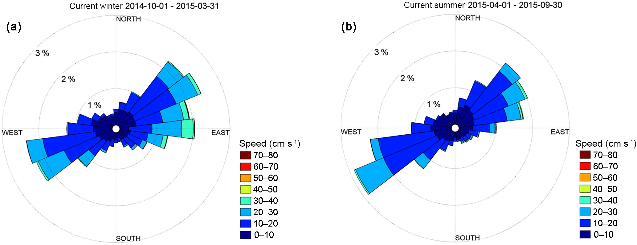
Figure 6 Current conditions in the storm season (a) from October 2014 to March 2015 and the summer season (a) from April 2015 to September 2015.

2.3.2 Recording current meter (RCM)

Continuous current data are available on PANGAEA for September 2014 to October 2015 (https://doi.org/10.1594/PANGAEA.877265). There are additional datasets before the main sampling period of November and December 2013, March 2014 and June 2014. These data were used as a basis for deciding on the final placement and orientation of the experimental islands. Gaps in the dataset are the result of local readouts and maintenance. Low-tide data were removed from the dataset. Data after October 2015 is missing due to sensor malfunctions. The structure of the datasets is shown in Table 3.

2.3.3 Tide and wave recorder (TWR)

Tide and wave data are available on PANGAEA from October 2014 to April 2017 (https://doi.org/10.1594/PANGAEA.877258). Gaps in the dataset are the result of local readouts and maintenance. Low-tide data were not removed from the dataset. The depth was calculated from raw pressure, which was corrected beforehand with atmospheric pressure. The structure of the datasets is described in Table 4.

2.3.4 Water level loggers (DL-W)

Data for groundwater level on the experimental islands and salt-marsh enclosed plots are available on PANGAEA from June 2015 to April 2017 (https://doi.org/10.1594/PANGAEA.877267). Gaps in the dataset are the result of local readouts and maintenance. For depth calculations, pressure data were manually corrected by atmospheric pressure. Each dataset includes date/time and water level (water level measured in m; Table 5).

2.3.5 Temperature loggers (DL-T)

Temperature data for the surface sediment layer of the experimental islands and salt-marsh enclosed plots are available on PANGAEA for September 2014 to April 2017 (https://doi.org/10.1594/PANGAEA.877257). Gaps in the dataset are the result of local readouts and maintenance. Each dataset includes date/time, depth in sediment (depth measured in m) and temperature in sediment (represented by t, expressed in degC; Table 6).

2.3.6 Light loggers (DL-L)

Measured light availability on the experimental islands and salt-marsh enclosed plots are available on PANGAEA from September 2014 to April 2017 (https://doi.org/10.1594/PANGAEA.877256). Gaps in the dataset result from local readouts and maintenance. Due to different calibrations for underwater or above-water application, raw data were processed differently and were merged depending on low- or high-water times. Each dataset includes the date/time and light intensity (Io, expressed in µmol m⁻² s⁻¹; Table 7).

2.3.7 Conductivity loggers (DL-C)

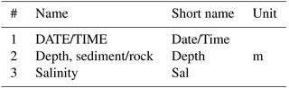
Data of conductivity measurements inside dip wells on the experimental islands and salt-marsh enclosed plots are available on PANGAEA for May 2015 to April 2017 (https://doi.org/10.1594/PANGAEA.877266). Gaps in the dataset result from local readouts and maintenance. Low-tide data were removed from the dataset. An automatic calculation of salinity were performed within the HOBOware Pro (V3.7.4) software according to PSS-78. Each dataset includes date/time, depth in sediment (depth measured in m) and salinity (Sal; Table 8).

Table 9 An overview of sensor and logger data availability over the 944-day sampling period. D 1 – sum of days with data available; D 0 – sum of days with data absent; % 1 – proportion of days with data available; % 0 – proportion of days with data absent; D x – total available days specified for each sensor application, i.e., from first deployment to last measurement; % x1 and % x0 are the corresponding percent availabilities. Sum 1 – number of measurements available; Sum 0 – number of measurements missing; % S 1 – proportion of measurements available; % S 0 – proportion of measurements missing; Sum x – total available measurements specified of each sensor application, i.e., from first data point to last measurement; %S x1 and %S x0 are the corresponding percent availabilities. WS: weather station, RCM: recording current meter, TWR: tide and wave recorder, DL: data logger.

3 Data availability

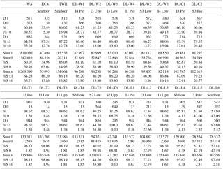
Sensor operation encompasses the time span of 32 months, from 18 September 2014 to 18 April 2017 (944 days). Figure 4 illustrates the data availability over the whole period, and Table 9 provides total availability in days as well as in percent.

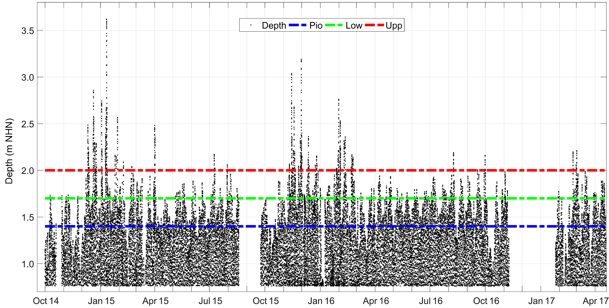
Figure 7 Calculated water depth (black dots) at 0.71 m NHN, next to islands 6 and 7. The blue line represents the elevation of the pioneer zone (Pio), the green line shows the height of the lower salt marsh (Low) and the red line describes the upper salt-marsh zone (Upp). Thus, water level data can give information about flooding periods at the three elevation levels. Low-tide data (all data below 0.05 m) were removed before plotting the data. To provide m NHN as a basis, 0.71 m were added to the data points.

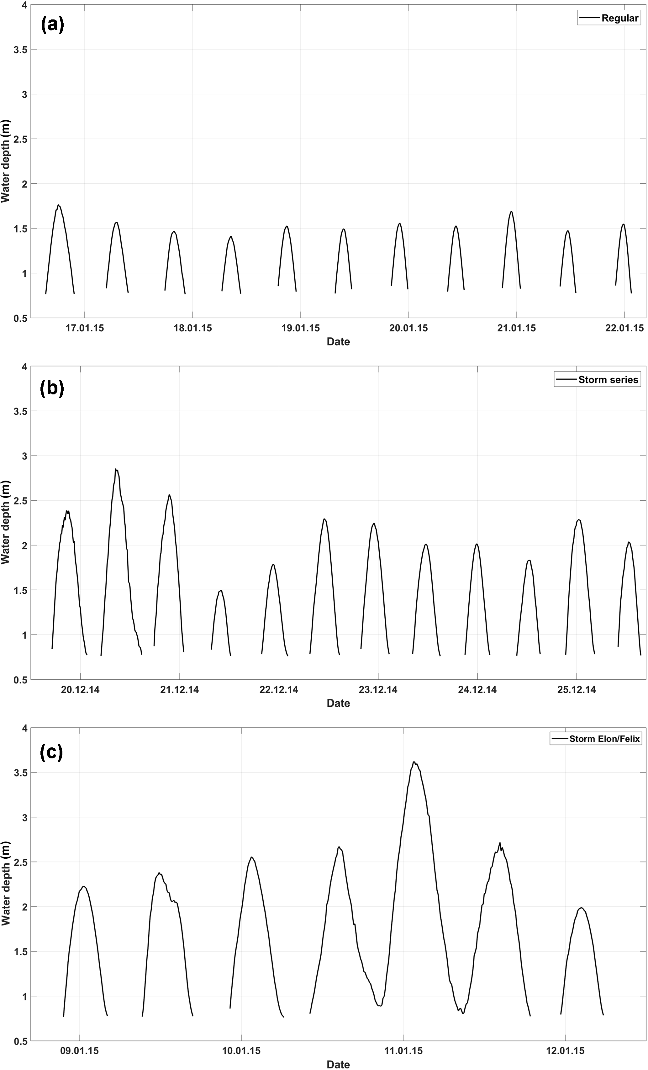
Figure 8 Calculated water depth (black line) during different weather conditions. (a) shows regular weather and wave conditions from 16 to 22 January 2015. (b) represents a series of storms with higher water levels from 19 until 25 December 2015. At this point the highest wave energy values were observed as well as highest significant wave heights. (c) shows the two big storms Elon and Felix, the latter occurring directly after the first storm. Here the highest water levels during application time were measured as well as the maximum wave height.

3.1 Weather station (WS)

Within this time frame meteorological data were available from 19 November 2014 to 18 April 2017 on 571 days (corresponding to 60.49 % availability). Absent days resulted from malfunctions and maintenances from 29 January 2015 to 11 March 2015, 4 November 2015 to 14 November 2015, 25 March 2016 to 28 October 2016 and 1 February 2017 to 21 March 2017.

3.2 Recording current meter (RCM)

Current meter operation was possible from 18 September 2014 until 6 October 2015 on 335 days (35.49 %). Further operations occurred in November and December 2013, March 2014, and June 2014 for preliminary investigations. Missing days were resulted from local maintenance and readouts. Due to a malfunction, the sensor had not been operating since October 2015.

3.3 Tide and wave recorder (TWR)

Continuous observations of wave and tide data were feasible from 1 October 2014 to 18 April 2017 on 812 days (corresponding to 86.02 % availability). Absent days were the result of local maintenance and readouts as well as some extended services from 19 October 2014 to 28 October 2014, 17 August 2015 to 23 September 2015 and 8 November 2016 to 24 January 2017.

Figure 9 Groundwater level on the experimental islands and the salt-marsh enclosed plot.

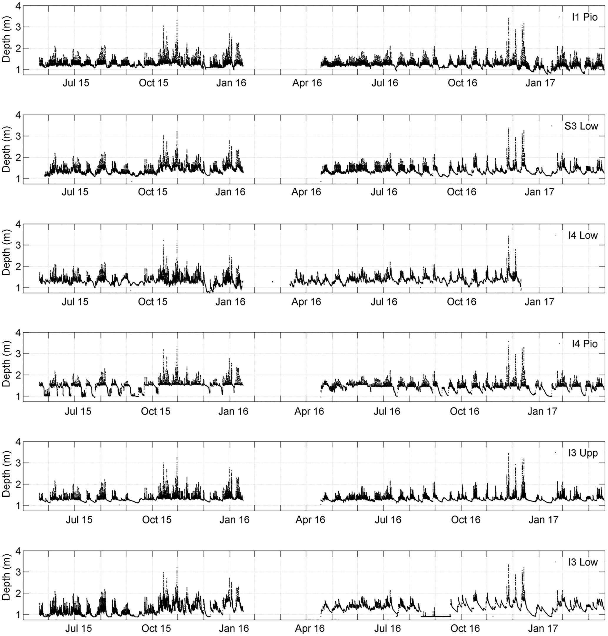
Figure 10 Surface layer temperature and temperature differences over the whole time frame with the DL-T2 (I3 Low).

3.4 Data logger (DL)

3.4.1 Water level loggers (DL-W)

Within the total time period water level measurements were performed from 20 June 2015 to 18 April 2017 on 578 days (572 days within the salt-marsh enclosed plot), resulting in a 61.23 % (60.59 %) availability. Absent days resulted from malfunctions and maintenances from 16 February 2016 to 18 May 2016 as well as some local readouts. Groundwater level data of the DEFI-D logger ends at 10 January 2017 due to a missing readout in April 2017. The coverage of water level measurements is therefore 50.85 % (480 days).

Table 10 Minima, maxima and mean values as well as median and standard deviation of the weather station (WS) for the time frame of 19 November 2014 to 18 April 2017 on 571 days. See Table 2 for parameter list.

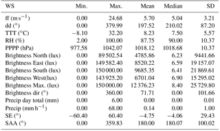
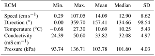
Table 11 Minima, maxima and mean values as well as median and standard deviation of the recording current meter (RCM) for its application time from 18 September 2014 until 6 October 2015 on 335 days.

3.4.2 Temperature loggers (DL-T)

Recordings of the surface layer temperature were available on 931 days, excluding the period from 10 January 2017 to 24 January 2017 due to maintenance (98.62 % availability). However, temperature data of two loggers within the salt-marsh enclosed plots (S2 Upp and S2 Low) exhibit a shorter time of deployment. An application was possible at 295/380 days (31.25 %/40.25 % availability) from 16 December 2014 to 6 October 2015 (S2 Upp and S2 Low) and further from 24 January 2017 to 18 April 2017 (S2 Low).

3.4.3 Light Loggers (DL-L)

Light intensity and availability was recorded over the whole period from 18 September 2014 to 18 April 2017 for 931 days, except for the period from 10 January 2017 to 24 January 2017 due to maintenance (98.62 % availability). Two loggers (I3 Pole, Seafloor) were first installed on 7 October 2015 with a total application time of 547 days, corresponding to 57.94 % availability. A light logger within the salt-marsh enclosed plot (S3 Low) had to be removed from 19 November 2014 to 16 December 2014 due to maintenance. A light logger on the experimental island (I3 Low) had to be temporarily removed between 23 September 2015 and 11 April 2016.

3.4.4 Conductivity Loggers (DL-C)

Data of the conductivity logger on the experimental island (I3 Pio) are available from 6 May 2015 to 16 February 2016 and from 18 May 2016 to 18 April 2017 on 624 days (66.10 % availability). The logger located in the salt-marsh enclosed plot (S3 Pio) recorded water conductivity from 7 May 2015 to 8 October 2015, 3 December 2015 to 16 February 2016 and from 18 May 2016 to 18 April 2017, 567 days in total (60.06 % availability). Gaps in the dataset resulted from a malfunction and maintenance.

Table 12 Minima, maxima and mean values as well as median and standard deviation of the tide and wave recorder (TWR) from 1 October 2014 to 18 April 2017 on 812 days.

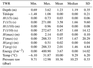
Table 13 Minima, maxima and mean values as well as median and standard deviation of the groundwater level data (DL-W 1-6) for each logger application time from 20 June 2015 to 18 April 2017 on 578 days (572 days within the salt-marsh enclosed plot).

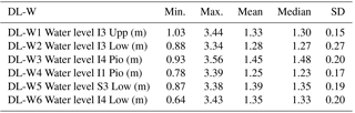
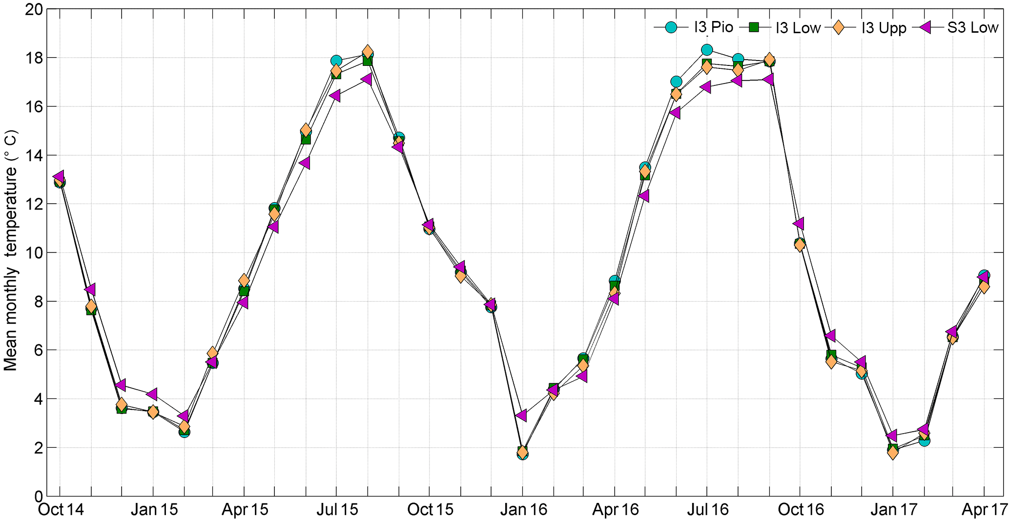
Figure 11 Mean monthly temperature over the whole application time. Since the temperatures on the experimental islands are very similar, a clear offset of the salt-marsh enclosed plot temperature could be identified in winter and summer months.

4 Results and discussion

4.1 Weather station (WS)

Local wind diagrams for three winter storm seasons and one summer season are shown in Fig. 5. Furthermore, minima, maxima and mean values as well as the median and standard deviation of the weather station for the time frame of 19 November 2014 to 18 April 2017 on 571 days are listed in Table 10. Within the application time, wind speeds of less than 25 m s⁻¹ were present. Mean wind speed was 5.7 m s⁻¹ ± 3.21, but it strongly differs between the single seasons.

4.2 Recording current meter (RCM)

Current conditions for one storm season and one summer season are shown in Fig. 6. A main current direction from the southwest to the northeast was clearly identified, showing the good orientation of the experimental islands. Furthermore, minima, maxima and mean values as well as the median and standard deviation of the RCM data from 18 September 2014 until 6 October 2015 on 335 days are listed in Table 11. A maximum current speed of 107.05 cm s⁻¹ was observed in December 2013 during storm Xaver. Mean current speed represent 12.9 cm s⁻¹ ± 8.62, but with variances between the single seasons.

Figure 12 Calculated sum of light intensity per day.

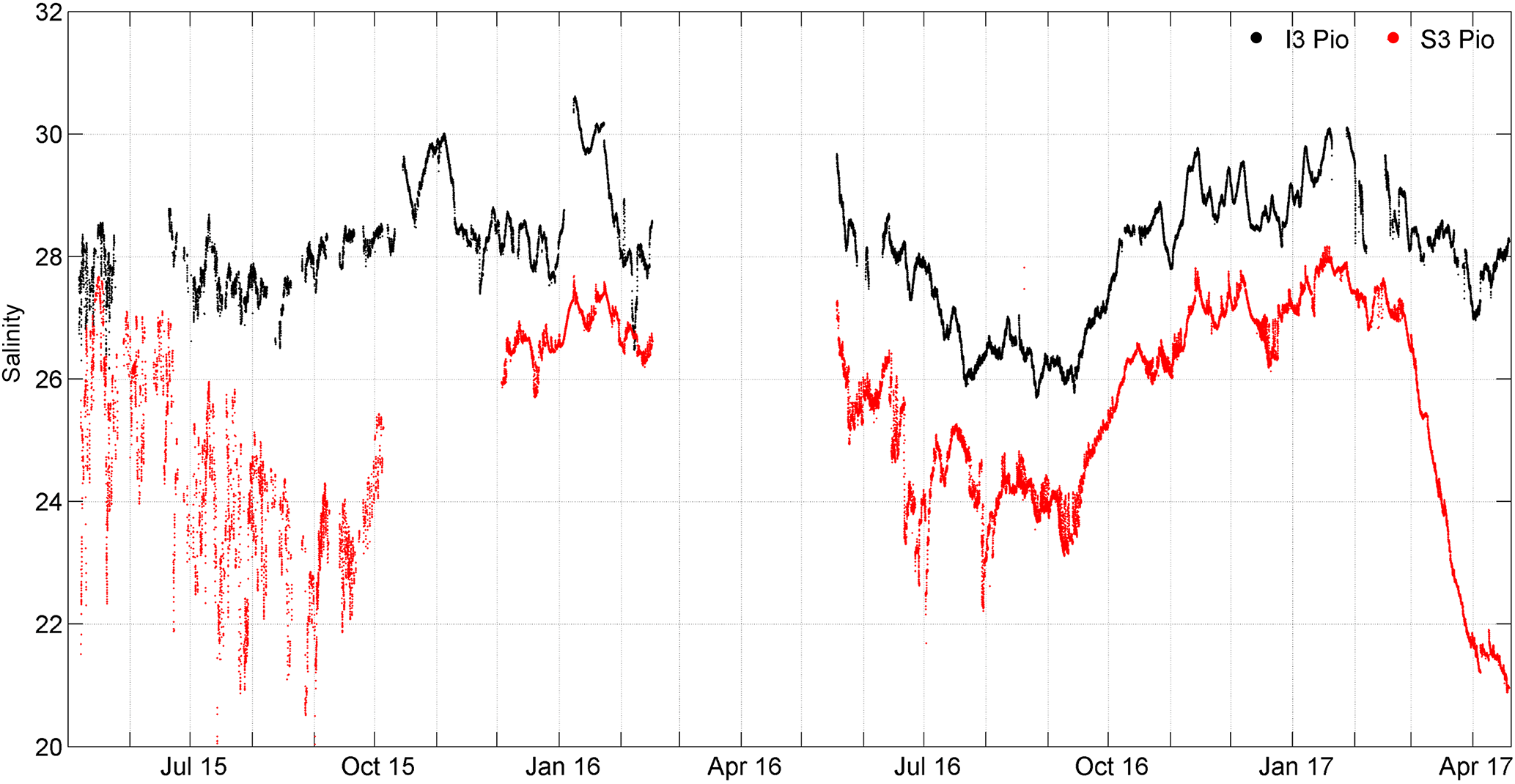
Figure 13 Salinity values within dip wells on the experimental island and salt-marsh enclosed plot. Due to fluctuations in the groundwater level, conductivity loggers periodically became dry, especially in the beginning. Thus, data until October 2015 are scattered. The depth of conductivity loggers was thereupon adjusted deeper in the dip wells, assuring a constant covering of water.

Table 14 Minima, maxima and mean values as well as median and standard deviation of the temperature data (DL-T 1-6) from 18 September 2014 until 18 April 2017 on 931 days.

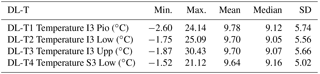
Table 15 Minima, maxima and mean values as well as median and standard deviation of the light intensity data (DL-L 1-6) for each logger application time.

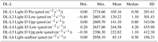
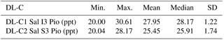
Table 16 Minima, maxima and mean values as well as median and standard deviation of the salinity data (DL-C 1-2) for each logger application time.

4.3 Tide and wave recorder (TWR)

The water depth calculated from pressure data of the tide and wave recorder (TWR) can be seen in Fig. 7. A seasonal pattern of water depth is exhibited and the highest water depths were reached during storm season. However, water level reached the upper salt-marsh zone (2.0 m NHN) several times (e.g., April 2015, July 2015 and August 2016). During the storms Elon and Felix in January 2015, the highest water level was observed at 3.62 m as well as the highest wave at 2.14 m (Fig. 8). The highest wave energy (400.90 J m⁻²) and significant wave height H(1/3), which was measured at 0.73 m, were detected during several shortly sequenced storm events in the weeks before in December 2014 (Fig. 8). Mean water depths for the whole application are 1.23 m ± 0.35 m. Statistic values of the TWR from 1 October 2014 to 18 April 2017 on 812 days are listed in Table 12.

4.4 Data logger (DL)

4.4.1 Water level loggers (DL-W)

The depth of the groundwater level achieved from pressure logger on the experimental islands and in the salt-marsh enclosed plots can be seen in Fig. 9. Differences in the water level were observed, especially during low water. This could be a result of various factors, ranging from diverse water consumption of plants to less flooding on higher elevations or leaks in the plastic bags inside an experimental island. Statistics of groundwater level data (DL-W 1-6) for each logger application time from 20 June 2015 to 18 April 2017 on 578 days (572 days within the salt-marsh enclosed plot) are listed in Table 13.

4.4.2 Temperature loggers (DL-T)

Surface layer temperatures for one experimental island and its three elevational zones as well as one elevation zone within the salt-marsh enclosed plots are shown in Fig. 10. To assess temperature differences the DL-T2 Logger (I3 Low) was taken to compare both differences within one island's elevational zone (DL-T1 I3 Pio, DL-T3 I3 Upp) and between the same elevational level and those of the salt-marsh control plots (DL-T4, S3 Low). All temperatures are very similar and showing only less differences, especially I3 Upp and I3 Low, with ΔT0.01±0.55 ^∘C. Since the temperatures on the experimental islands are very similar considering the mean monthly temperatures of the four plots, a clear offset of the salt-marsh enclosed plot temperature could be identified in winter and summer months (Fig. 11). The lowest temperature was observed at I3 Pio with −2.6 ^∘C, whereas the highest value of 30.43 ^∘C was measured at the upper zone of the experimental island. Maximum temperatures of S3 Low and I3 Upp differ by 9.31 ^∘C. Mean values are very similar and ranging from 9.64 ^∘C ± 5.02 (S3 Low) to 9.78±5.74 (I3 Pio). More statistics of temperature data (DL-L 1-6) for each logger application time from 18 September 2014 to 18 April 2017 on 931 days are listed in Table 14.

4.4.3 Light loggers (DL-L)

To calculate the light sum per day, measured light intensity (Quantum (µmol m⁻² s⁻¹)) was extrapolated from seconds to the measuring interval of 10 min, and afterwards values were added up for 1 day. Polycarbonate covers were installed on the experimental islands to prevent the scouring during the storm season (Balke et al., 2017). In consequence, lower light availabilities were detected under the covers (Fig. 12) at island 3 in I3 Pio, I3 Low and I3 Upp other than at the seafloor, I3 Pole and S3 Low (all uncovered). Minima, maxima and mean values as well as the median and standard deviation of the light intensity data (DL-L 1-6) for each logger application over the whole period from 18 September 2014 to 18 April 2017 for 931 days are listed in Table 15.

4.4.4 Conductivity loggers (DL-C)

Salinity values achieved from both conductivity logger on the experimental island and the salt-marsh enclosed plot can be seen in Fig. 13. Due to fluctuations in the groundwater level, conductivity loggers periodically became dry, especially in the beginning. Thus, data until October 2015 are scattered. The conductivity loggers were thereupon adjusted deeper in the dip wells assuring a constant covering of water. The mean salinity for the experimental island is 27.95 ± 1.22 and 25.45 ± 1.74 for the salt-marsh enclosed plot. Both loggers were installed at the pioneer zone. Statistics of salinities (DL-C 1-2) for each logger application time from 6 May 2015 to 16 February 2016 and from 18 May 2016 to 18 April 2017 on 624 days are shown in Table 16.

6 Conclusions and future directions

The BEFmate project included a variety of experiments dedicated to investigate biodiversity–ecosystem functioning across marine and terrestrial ecosystems, utilizing 12 experimental islands in the back-barrier tidal flat of Spiekeroog Island. Abiotic conditions were recorded from a suite of 23 different sensors installed at different locations in the vicinity of the experimental islands, on the islands themselves and in the nearby salt marsh. Data described here covers the period from September 2014 to April 2017 and has been published in seven datasets in the World Data Center PANGAEA. Data coverage within the period ranged from 35 % for the recording current meter (RCM) that failed in October 2015 to 99 % for six data loggers. With 17 sensors covering 80 % or more of the period of interest, a very good coverage was achieved. Additional data from pre-experiment investigations with the RCM between November 2013 and June 2017 was added to the dataset. Seasonal and tidal dynamics as well as storms were covered, and these data are available for interpretation in further contexts.

For future operations, data availability can be further increased if a rotational system for maintenance is applied, provided that spare sensors are available. Furthermore, the online data transfer of central information would not only increase the data availability, but meteorological and hydrographic conditions could also indicate the need to attend the experiment. For example, indicating a need to take action to prevent damage during extreme weather events. Non-invasive remote sensing sensor techniques can provide complementary data, to avoid fouling issues, as demonstrated successfully at the nearby Time Series Station – Spiekeroog (Garaba et al., 2014; Schulz et al., 2016). Additionally camera systems should be applied, providing a visual impression of the overall scene and detailed information, e.g., the process of flooding for different levels. Recently the RCM failure within the BEFmate project has inspired the development of a machine-learning environment that creates a virtual sensor enabling the compensation for single sensor dropouts (Oehmcke et al., 2017a, b). Finally, data quality assurance and quality measures should be further developed to reduce the workload of manual data curation while improving data availability in near-real time.