the Creative Commons Attribution 4.0 License.
the Creative Commons Attribution 4.0 License.
 | 13 Sep 2018
Deriving a dataset for agriculturally relevant soils from the Soil Landscapes of Canada (SLC) database for use in Soil and Water Assessment Tool (SWAT) simulations
Marcos R. C. Cordeiro
Glenn Lelyk
Roland Kröbel
Getahun Legesse
Monireh Faramarzi
Mohammad Badrul Masud
The Soil and Water Assessment Tool (SWAT) model has been commonly used in Canada for hydrological and water quality simulations. However, preprocessing of critical data such as soils information can be laborious and time-consuming. The objective of this work was to preprocess the Soil Landscapes of Canada (SLC) database to offer a country-level soils dataset in a format ready to be used in SWAT simulations. A two-level screening process was used to identify critical information required by SWAT and to remove records with information that could not be calculated or estimated. Out of the 14 063 unique soil records in the SLC, 11 838 records with complete information were included in the dataset presented here. Important variables for SWAT simulations that are not reported in the SLC database (e.g., hydrologic soils groups (HSGs) and erodibility factor (K)) were calculated from information contained within the SLC database. These calculations, in fact, represent a major contribution to enabling the present dataset to be used for hydrological simulations in Canada using SWAT and other comparable models. Analysis of those variables indicated that 21.3 %, 24.6 %, 39.0 %, and 15.1 % of the soil records in Canada belong to HSGs 1, 2, 3, and 4, respectively. This suggests that almost two-thirds of the soil records have a high (i.e., HSG 4) or relatively high (i.e., HSG 3) runoff generation potential. A spatial analysis indicated that 20.0 %, 26.8 %, 36.7 %, and 16.5 % of soil records belonged to HSG 1, HSG 2, HSG 3, and HSG 4, respectively. Erosion potential, which is inherently linked to the erodibility factor (K), was associated with runoff potential in important agricultural areas such as southern Ontario and Nova Scotia. However, contrary to initial expectations, low or moderate erosion potential was found in areas with high runoff potential, such as regions in southern Manitoba (e.g., Red River Valley) and British Columbia (e.g., Peace River watershed). This dataset will be a unique resource to a variety of research communities including hydrological, agricultural, and water quality modelers and is publicly available at https://doi.org/10.1594/PANGAEA.877298.
- Article
(660 KB) - Full-text XML
-
Supplement
(129 KB) - BibTeX
- EndNote


Integrated environmental modeling is inspired by modern environmental problems and enabled by transdisciplinary science and computer capabilities that allow the environment to be considered in a holistic way (Laniak et al., 2013). In an agricultural context, synthesis and quantification of multidisciplinary knowledge via process-based modeling are essential to manage systems that can be adapted to continual change (Ahuja et al., 2007). The Soil and Water Assessment Tool (SWAT) (Arnold et al., 1998) is an example of such a process-based model. It has been developed over the past 30 years to evaluate the effects of alternative management decisions on water resources and nonpoint-source pollution in large river basins through the simulation of major processes including hydrology, soil temperature and properties, plant growth, nutrient and pesticides dynamics, bacteria and pathogens transport, and land management (Arnold et al., 2012; Douglas-Mankin et al., 2010). Furthermore, a weather generator is included in the model to fill gaps that may exist in meteorological records.
The SWAT model has been extensively tested around the world for a wide range of hydroclimatic conditions, water and land management practices, and timescales (Douglas-Mankin et al., 2010; Arnold et al., 2012; Gassman et al., 2014). The wide adoption of the SWAT model has been prompted by preprocessing and post-processing software tools such as a GIS interface and extensive user documentation (Arnold et al., 2012), as well as several linked databases for crops, soils, fertilizers, tillage, and pesticides (Santhi et al., 2005). Among these, soil properties are especially important as they are needed for the simulation of influential processes such as evapotranspiration, soil water balance, nutrient dynamics, and sediment transport (Neitsch et al., 2005). However, the existing built-in database is only valid for SWAT applications in the USA. Accordingly, studies outside the USA require the development of a soils dataset by preprocessing available soils data into a format readable by SWAT, a time-consuming process as not all data required by SWAT are readily available for countries outside of the USA.
Worldwide, SWAT has emerged as one of the most widely used water quality watershed- and river-basin-scale models for simulation of a broad range of hydrologic and/or environmental problems (Gassman et al., 2014). These applications in different regions are described in the extensive body of peer-reviewed SWAT literature (Arnold et al., 2012). Specifically in Canada, the SWAT model has been used for hydrological simulations in most provinces, including Prince Edward Island (Edwards et al., 2000), New Brunswick (Chambers et al., 2011; Yang et al., 2009), Nova Scotia (Ahmad et al., 2011), Ontario (Asadzadeh et al., 2015; Rahman et al., 2012), Quebec (Lévsque et al., 2008), Manitoba (Yang et al., 2014), Saskatchewan (Mekonnen et al., 2016), Alberta (Mapfumo et al., 2004; Watson and Putz, 2014; Faramarzi et al., 2015), and British Columbia (Zhu et al., 2012). However, preparation of Canadian soils information in a consistent and usable format for SWAT is time-consuming (Rahman et al., 2012), as information has to be collected from soil reports and cross-checked against GIS datasets, missing soil variables have to be calculated from other physical and hydraulic properties, and all parameters have to be attributed to specific soil grids or polygons.
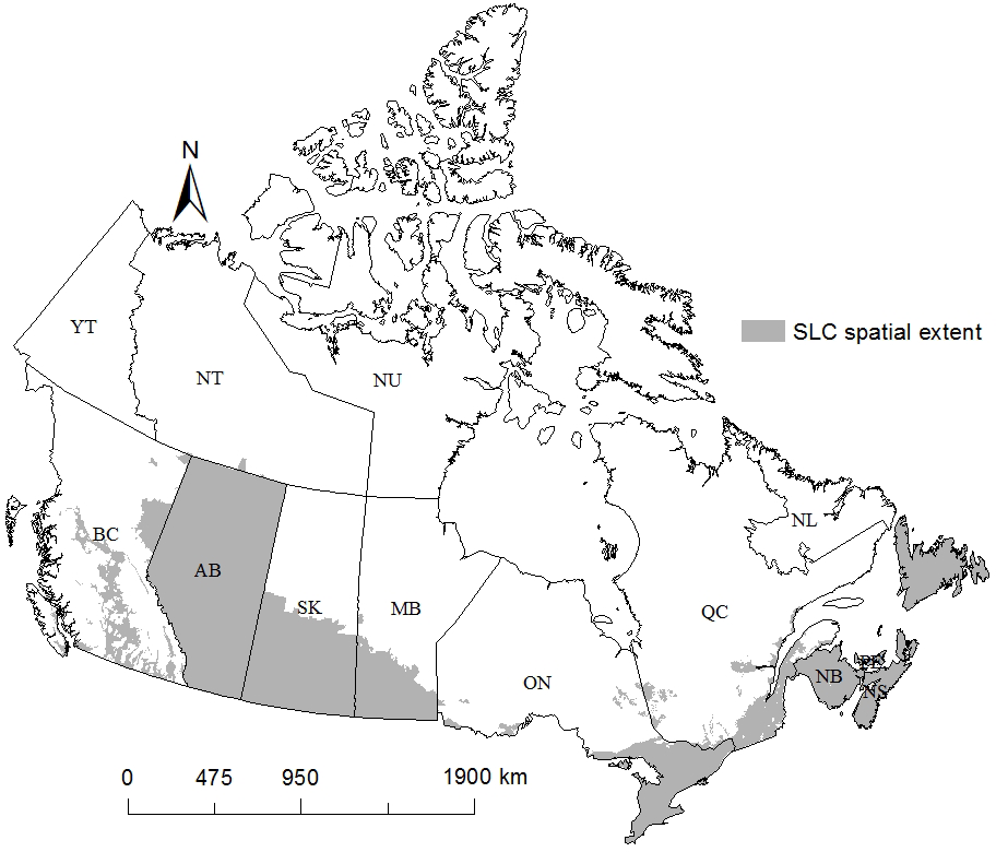
Figure 1Spatial extent of the Soil Landscapes of Canada (SLC) database showing coverage in the provinces of Newfoundland and Labrador (NL), Prince Edward Island (PE), Nova Scotia (NS), New Brunswick (NB), Quebec (QC), Ontario (ON), Manitoba (MB), Saskatchewan (SK), Alberta (AB), and British Columbia (BC), as well as the Northwest Territories (NT).
Some of this preprocessing work can be alleviated by using publically available databases that contain most of the information required by SWAT. The Soil Landscapes of Canada (SLC) database published by Agriculture and Agri-Food Canada (Soil Landscapes of Canada Working Group, 2010) is an example, and has been used in SWAT applications in Ontario (Asadzadeh et al., 2015; Rahman et al., 2012), Saskatchewan (Mekonnen et al., 2016), Alberta (Faramarzi et al., 2015), and British Columbia (Zhu et al., 2012). The SLC contains a GIS dataset series that provides information about the country's agricultural soils at the provincial and national levels. It was compiled at a scale of 1 : 1 million, and the information is organized according to a uniform national set of soil and landscape criteria based on permanent natural attributes (Soil Landscapes of Canada Working Group, 2010). The SLC encompasses the southern portions of the provinces of Ontario and Quebec and a larger portion of the Prairies provinces of Manitoba, Saskatchewan, and Alberta as far north as to the boreal shield. Coverage in the maritime provinces of New Brunswick, Nova Scotia, and Prince Edward Island is nearly complete (Fig. 1).
Although there are more detailed soil datasets available at provincial levels (e.g., AGRASID dataset in Alberta), selection of SLC for integration with SWAT was based on the fact that (i) it covers most soils across the agricultural regions of Canada in a single dataset; (ii) it has been used in regional studies in Canada, as described above; and (iii) it is more easily applicable to large-scale national studies as broad-scale datasets require reduced resources to prepare and process data (Moriasi and Starks, 2010). Modeling studies comparing the performance of a single model (calibrated and uncalibrated) but using soil datasets with varying spatial resolution in the USA (i.e., the State Soil Geographic database (STATSGO) compiled at 1 : 250 000 scale, and the Soil Survey Geographic database (SSURGO) with scales ranging from 1 : 12 000 to 1 : 63 360) also revealed that using either dataset produced comparable results (Mednick, 2008).
Besides the American databases (i.e., STASTSGO and SSURGO), the authors are not aware of any other effort to produce a similar dataset from a national soils database for specific use with SWAT, such as the one presented here for Canada. Past efforts in preparing a large-scale soils dataset for modeling include the standardization of the FAO–UNESCO, but this dataset was not optimized for SWAT and is presented at a much coarser spatial resolution (i.e., 1 : 5 000 000; Batjes, 1997). The SOTER (Soil Terrain) database is another initiative to provide a global soils dataset, which was intended to have a global coverage at 1 : 1 million scale but was later degraded to 1 : 5 million scale due to the lack of means (Dobos et al., 2005). However, SOTER is not optimized for SWAT use and requires some variables to be calculated or estimated to this end (Bossa et al., 2012). Other databases at continental scale, such as the HYPRES in Europe, only cover soil hydrologic properties (Wösten et al., 1999). At national level, only a few countries besides the USA and Canada have a soil electronic database (e.g., Australia, Brazil, and China; Shi et al., 2004; Cooper et al., 2005), while these data are not available in most countries (Cooper et al., 2005). The reduced number of available datasets, coupled with the technicalities involved in translating these datasets into SWAT format and the required variables not reported in them, contribute to the lack of large-scale soil databases fully compatible with SWAT. These limitations emphasize the novelty and importance of the dataset presented in this paper. Besides presenting a soils database ready to use in SWAT simulations in Canada, the present work provides a framework to support similar initiatives in other regions using data from global soil databases.
Table 1Description of variables in SWAT's “usersoil” table.
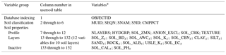
* Subscript x corresponds to soil layer from 1 to 10.
Due to the importance of the SWAT model for integrated environmental modeling in Canada, and the prominence of the SLC database as a potential input dataset for this model at a national level, the objective of this work was to offer a country-level soils dataset in a format ready to be used in SWAT simulations. The dataset was derived to provide over 20 parameter values for different soil types that are varied for each soil layer. It was prepared in a format suitable for use in the ArcSWAT version of the model, which is attributed to a grid or polygon-based soil map. Such a laborious preprocessing exercise is widely, but inconsistently, adopted in SWAT simulations reported in the literature. Finally, deficiencies in the dataset are also presented and discussed.
The SLC database (http://sis.agr.gc.ca/cansis/nsdb/slc/v3.2/index.html, last access: 20 June 2017) is structured as a component-based GIS layer, whereby a single polygon may contain several soil records. This structure is similar to that of the State Soil Geographic (STATSGO) database in the USA (Srinivasan et al., 2010). Such structure creates a one-to-many relationship, whereby the multiple soil components of a polygon are not spatially defined. The actual soil information in the SLC database is stored in a number of tables linked together through intricate relationships (Soil Landscapes of Canada Working Group, 2010). Among these, four tables are relevant for developing a dataset for SWAT applications:
-
The Polygon Attribute Table (PAT) provides the linkage between geographic locations (polygons in the SLC GIS coverage) and soil landscape attributes in the associated database tables (e.g., unique soil ID in the Soil Name Table (SNT) and respective number of layers in the Soil Layer Table (SLT)).
-
The Component Table (CMP) describes each of the individual soil and landscape features comprising the polygons. That is, it describes which soil records are present in each spatial unit (i.e., polygon) in the GIS layer.
-
The Soil Name Table (SNT) describes the general physical and chemical characteristics for all of the soils identified in a geographic region.
-
The Soil Layer Table (SLT) contains soil information that varies in the vertical direction (i.e., layered attributes).
The CMP table describes the proportion of each nonspatially defined soil component in a polygon if more than a soil component exists (the soil component(s) refers to the soil(s) element(s) that comprise each polygon). The component numbering follows a sequence of decreasing proportion in a polygon (i.e., first component has the highest proportion; last component has the smallest proportion). This component-based structure of the SLC database does not affect the analysis since all the soil records listed in the SNT table were processed to generate the present dataset. However, it has implications for the SWAT model user, who has to make a decision on how to handle the relationship between the polygon (spatially defined) and each nonspatially defined soil component in multicomponent polygons (e.g., selecting the larger component in a polygon or generating a hybrid soil incorporating properties of each soil component).
The SWAT soils information is stored in the “usersoil” table, located within the SWAT 2012 database in Microsoft Access format (i.e., SWAT2012.mdb). Each soil record is stored as a new record (i.e., row) in the table. Specific soil variables (Table 1) comprise the 152 columns of the usersoil table. The first column is an OBJECTID field assigning a unique identifier for each record. Columns two through six pertain to soil classification. The second column is the map unit identifier (MUID), which is used for mapping a collection of areas grouped by the same soil characteristics. A single MUID may describe different soil types, which are stored with a record counter in the third column (SEQN), while a soil identifying name (SNAM), a soil interpretation record (S5ID), and the percent of each soil component (CMPPCT) are recorded in the fourth, fifth, and sixth columns, respectively (Sheshukov et al., 2009). Columns 7 through 12 describe major soil properties pertaining to the soil record, namely, the number of layers (NLAYERS), the hydrological soil group to which that soil belongs (HYDGRP), the maximum rooting depth of the soil profile (SOL_ZMX), the fraction of soil porosity from which anions are excluded (ANION_EXCL), the potential of maximum crack volume of the soil profile expressed as a fraction of the total soil volume (SOL_CRK), and the texture of the soil layer (TEXTURE).
The next 120 columns starting from column 13 (i.e., columns 13 to 132) describe the information for each layer of the soil record. These columns are arranged in sets of 12 variables each for 10 possible soil layers. The variable NLAYERS indicates how many of these sets should be populated. Variables for any sets beyond NLAYERS should be assigned a value of zero. The variables included in each set of soil layers are the depth from the soil surface to the bottom of the layer (SOL_Z), moist bulk density (SOL_BD), available water capacity of the soil layer (SOL_AWC), saturated hydraulic conductivity (SOL_K), organic carbon (SOL_CBN), clay (CLAY), silt (SILT), sand (SAND), and rock fragment (ROCK) contents, moist soil albedo (SOL_ALB), erodibility factor (USLE_K), and electrical conductivity (SOL_EC). Beyond the columns describing layered soil information, there are 20 columns (i.e., columns 133 to 152) describing two variables (i.e., soil CaCO3 (SOL_CA) and soil pH (SOL_PH)) for 10 soil layers. These variables are not currently active in SWAT and are assigned a value of zero.
Despite its usefulness as a source of soil information for hydrological simulations, the SLC dataset is not assembled in a format readable by SWAT or other similar models. For example, SWAT stores all the properties for a specific soil record in a single row in the usersoil table, while this information is stored in the SLC as multiple rows in two different tables (i.e., SNT and SLT). Thus, the information contained in the SLT database has to be processed to satisfy SWAT's format requirements. In addition, all properties in the usersoil table are spatially defined, while those of SLC are often stored in a multi-polygon structure with no unique spatial identification. Variables required by SWAT and contained in the dataset presented here were either extracted from SNT and SLT, or calculated from the information therein. Some other variables were estimated from published values. Extraction or calculation of variables was done through an R code that imported both SNT and SLT, screened the data for missing records and missing SWAT-required information (data screening is described in Sect. 5), and sequentially populated unique soil records in the database. The next section describes how these variables were defined.
Table 2Variables included in the SWAT usersoil table.
Adapted from Arnold et al. (2013) and Sheshukov et al. (2009). a Subscript x corresponds to soil layer from 1 to 10. The variables SOL_CALx and SOL_PHx are present in the usersoil table after all the columns listed above for all the 10 preexisting layers. These variables refer to soil CaCO3 and soil pH, respectively, and are not currently active in the model. Thus, their records are entered as zero in the SWAT 2012 database. b The number of layers defines how many entries will be required in the layered information, signalled by the subscript x. For example, a soil with NLAYERS = 4 should have subscript x corresponding to soil layer variables from 1 to 4. As a result, the records extend to column 60 in the usersoil table. (i.e., 4 layers × 12 variables + 12 preceding variables = 60).
5.1 Screening out incomplete soil information in the SNT
The use of the SNT is necessary as it links the soils information to the GIS coverage containing the PAT. However, a first screening was required to remove soil records from the SNT that are not present in the SLT, as soil layer information is required by SWAT. The mismatch among soil records in both tables can occur for a number of reasons. For example, there are records in both tables that pedologists have identified but whose properties have not yet been characterized. Also, soil records listed in one table may be absent from another table due to changes in soil classification. Finally, soil records listed as unclassified in the SNT (i.e., variable KIND = U) do not have any data associated with them in the SLT and do not occur on any published map.
Out of the 14 063 unique soil records in the SNT, 489 were missing in the SLT and, therefore, removed from the analysis. These 489 soil records correspond to around 3.5 % of the soils listed in the SNT. Most of the missing records were reported as unclassified (305 soils; 62.2 %), suggesting that these soils have been identified, but their properties have not yet been characterized. Mineral soil records corresponded to 29.4 % (144 soils) of the total, likely a reflection of changes in classification. The other two classes comprised non-true soils (e.g., mine tailings, urban land; 33 soils; 6.7 %) and organic soils (8 soils; 1.6 %). Also, only 58 of the 489 missing soil records (11.0 %) could be mapped through linking with the CMP table, making it impossible to do any spatial analysis on the distribution of these soils across the country. However, since the SNT assigns a province for each soil record, it is possible to identify where these missing records occur. Most of the missing soil records were in British Columbia (167 soils; 34.2 %), Manitoba (151 soils; 30.9 %), and Saskatchewan (133 soils; 27.2 %), with smaller proportions in Yukon (13 soils; 2.7 %), Ontario (11 soils; 2.3 %), Nova Scotia (9 soils; 1.8 %), and Newfoundland (5 soils; 1.0 %).
5.2 SWAT requirements
The SWAT data requirements were used as a second level of screening to build the present dataset. The soil input variables in SWAT can be either required or optional (Table 2; Arnold et al., 2013). Required variables that could not be calculated or estimated (e.g., SOL_BD, SOL_K, SOL_CBN, CLAY, SILT, and SAND) were used to separate complete from incomplete records. Soil records in the SLT containing or allowing derivation of all the variables required by SWAT were compiled in a dataset comprising 11 838 unique records that were importable into the model. Soils in the SLT with missing records (i.e., variables entered as −9 in the database) for the required SWAT variables (gray rows in Table 2) were removed from the analysis. These soil records were compiled into a soils list provided as a reference.
As for the nonmatching soil records in the SNT and SLT, only 547 out of 1736 (i.e., 31.5 %) records with missing information could be mapped through linking with the CMP table, which renders any spatial representation of these records nonmeaningful. However, the provinces where these records occur could also be identified. The highest proportions of soil records with incomplete information were in British Columbia (490 records; 28.2 %) and Manitoba (391 records; 22.54 %). Ontario (182 records; 10.5 %) and Alberta (180 records; 10.4 %) had intermediate values, while Newfoundland (123 records; 7.1 %), Saskatchewan (102 records; 5.9 %), New Brunswick (93 records; 5.4 %), the Northwest Territories (80 records; 4.6 %), Nova Scotia (47 records; 2.7 %), Quebec (30 records; 1.7 %), and Yukon (17 records; 1.0 %) had less than 10 % of the soil records missing information.
The variables in SWAT's usersoil table refer to record indexing and soil classification, as well as soil properties pertaining to the entire profile or specific layers. The variables in each of these groups are described in the following subsections. The usersoil table starts with a number of columns that define the database and soil classification variables, followed by soil profile and layer information, and inactive soil properties (Table 2).
6.1 Database and soil classification variables
The SWAT soil classification variables include the OBJECTID (general listing number), MUID (map unit identifier), SEQN (sequence number), SNAM (soil name), S5ID (Soils5 ID number for USDA soil series data), and CMPPCT (percentage of the soil component in the MUID). A numbering system used for the OBJECTID variable was chosen to avoid conflicts with existing soil records in the usersoil table. The SWAT model comes with more than 200 soil records in a built-in database that cannot be easily overwritten, and any soil record imported into the database with the same OBJECTID as the existing record will not be imported. Thus, the OBJECTID field was populated sequentially from 1001 to the number of unique soil records in the SLC database plus 1000 (i.e., OBJECTID ends in 12 838 in the case of the COMPLETE dataset, which has 11 838 unique soil records). The map unit ID (MUID) was assigned the SOIL_ID code in the SLC dataset, which is a concatenation of the province code (two digits), a soil code (three digits), a modifier code (five digits), and a profile code (one digit). The sequence number (SEQN) variable was assigned the same value as the OBJECTID variable. This process created a unique SEQN for each recurrence in the SLC dataset.
Similar to the MUID variable, the soil name variable (SNAM) was also assigned the SOIL_ID code in the SLC, despite the soil name being in the database, so as to link the soil information to the GIS layer. The S5ID variable was created as a concatenation between the acronym “SLC” and the province two-digit abbreviation code. For example, all the soil records in the province of Alberta have an S5ID equal to “SLCAB”. The CMPPCT variable was assigned a value of 100, meaning that the soil comprises 100 % of this component. As stated in Sect. 2, the user has to make a decision on how to handle multipart polygons in the preprocessing of the SLC GIS dataset since the soil records in multicomponent polygons are not spatially defined.
6.2 Soil profile information
The following six variables in the dataset (i.e., columns 7 to 12) pertain to soil profile information. The number of layer variables (NLAYERS) was defined according to the soil layers in the SLT below the soil surface. The SLT table also contains information for layers above the soil surface, as is the case for litter, which have negative values for upper and lower depths (i.e., the ground surface corresponded to the zero depth, while above-surface and below-surface layers have negative and positive values, respectively). Above-surface layers were removed from the dataset prior to analysis through filtering layers with lower depth above the soil surface (i.e., lower depth less than or equal to zero).
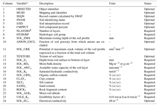
The hydrologic soil group (HSG) variable (HYDGRP) is an influential parameter for estimation of runoff using the SCS curve number method and, consequently, for hydrological simulations in SWAT (Gao et al., 2012; Neitsch et al., 2005). The HSGs were calculated according to the method outlined by USDA-NRCS (1993), which is based on depth to the impermeable layer (e.g., bedrock), depth from soil surface to shallowest water table during the year, hydraulic conductivity of the least conductive layer of the soil profile, and depth range of the hydraulic conductivity. The specific criteria used are provided in tabular form in the Supplement. Soils in the dual HSG classes were assigned to the less restrictive class since most agricultural areas in Canada exhibit some degree of drainage (e.g., municipal drainage network, surface drains, or tile drainage). SWAT translates HSG alphabetical classification into a numeric system, where HSGs A, B, C, and D, are interpreted as 1, 2, 3, and 4, respectively. The runoff potential increases with increasing numeric designations.
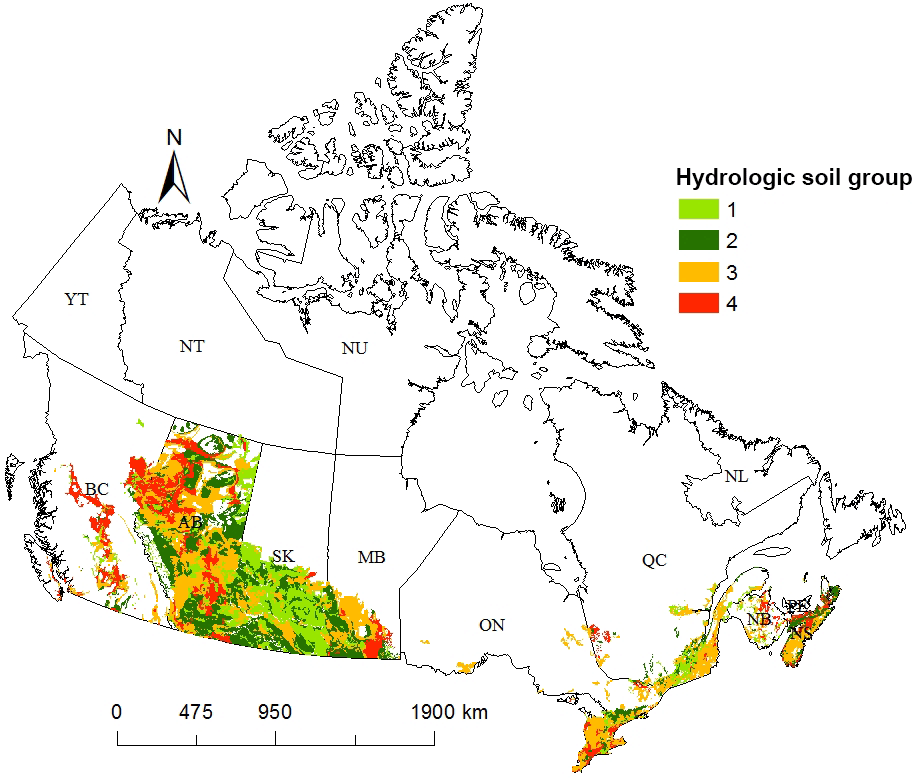
Figure 2Spatial distribution of the hydrologic soil groups (HYDGRP) variable calculated for the Soil Landscapes of Canada (SLC) database. HSG A = 1, HSG B = 2, HSG C = 3, and HSG D = 4 shown for the provinces of Prince Edward Island (PE), Nova Scotia (NS), New Brunswick (NB), Quebec (QC), Ontario (ON), Manitoba (MB), Saskatchewan (SK), Alberta (AB), and British Columbia (BC). Some HSGs could not be mapped (e.g., province of Newfoundland and Labrador (NL)) due to missing records in the PAT of the GIS layer or being part of the soils with missing data in the SLT.
The depth to the impermeable layer is not reported in the SLC database and was estimated based on the soil layers available in the SLT. When a bedrock layer or specific soil horizons were present (i.e., fragipan; duripan; petrocalcic; ortstein; petrogypsic; cemented horizon; densic material; placic; bedrock, paralithic; bedrock, lithic; bedrock, densic; or permafrost; USDA-NRCS, 1993), its upper depth was used as the depth to impermeable layer. When a bedrock layer was absent, the lower depth of the deepest mineral soil layer was used as an alternative. The shallowest annual depth to water table is also not reported and was estimated based on drainage class reported in the SNT. Very poorly drained, poorly drained, imperfectly drained, moderately well drained, and well drained (or better) soils were assigned water table depths of 0, 25, 75, 100, and 125 cm, respectively. The variables pertaining to hydraulic conductivity of the least conductive layer of the soil profile and depth range of the hydraulic conductivity were both calculated using information from the SLT.
Out of the 11 838 soil records in the generated dataset, 21.3 %, 24.6 %, 39.0 %, and 15.1 % belonged to HSGs 1, 2, 3, and 4, respectively. These results suggest that more than half of the agricultural soil records in Canada have a relatively high or high runoff generation potential (i.e., HSGs 3 and 4, respectively). A spatial analysis indicated that 20.0 %, 26.8 %, 36.7 %, and 16.5 % of the areal extent of the soil records belonged to HSGs 1, 2, 3, and 4, respectively. Many of the soil records with higher potential for runoff generation are in the humid regions of Ontario, Quebec, and the Maritimes (Fig. 2). Not surprisingly, this region has extensively adopted measures to address excess moisture in agricultural soils, such as tile drainage (Stonehouse, 1995; Rasouli et al., 2014). Excess moisture is also a problem in areas of Canadian Prairies, such as the Red River Valley in Manitoba, where surface drainage (Bower, 2007) and a growing use of tile drainage (Cordeiro and Sri Ranjan, 2012, 2015) have been used to address this problem. Conversely, soil records with low potential for runoff generation are located in Saskatchewan and southeastern Alberta (along the Saskatchewan border), which are among the most arid regions in Canada (Wolfe, 1997).
The maximum rooting depth of the soil profile (SOL_ZMX) was assumed to be the lower depth of the deepest layer in the SLC soil profile. The fraction of soil porosity from which anions are excluded (ANION_EXCL) was not available in the SLC database and was set to the default value of 0.5 in SWAT (Arnold et al., 2013). This variable affects the concentration of nitrate in the mobile water fraction, which is directly related to nitrate leaching. The potential of maximum crack volume of the soil profile expressed as a fraction of the total soil volume (SOL_CRK) can be calculated with the FLOCR model using 30-year weather data (Bronswijk, 1989). However, due to the fact that the model is not readily available for download and the unreasonable time required to run the model for such a large number of soil records, as well as the fact that SOL_CRK is optional in SWAT, its value was set to 0.5. In large-scale studies this value is further adjusted through a spatially explicit calibration scheme (Whittaker et al., 2010). The SOL_CRK variable controls the potential crack volume for the soil profile. This value was selected based on the fact that all of the built-in soil records in the SWAT soils database have the SOL_CRK variable set to 0.5. The TEXTURE variable, although not required for simulations with the SWAT model, was estimated for reference using the “TT.points.in.classes” function from the “soiltexture” R package (Moeys, 2016). The Canadian soil texture classification system was used as a reference.
6.3 Soil layer information
The soil profile variables are followed by 10 sets of 12 variables (i.e., columns 13 to 132) pertaining to layered soil information. The lower depth of each soil layer in the SLT was used as the depth from soil surface to the bottom layer (SOL_Z). The soil bulk density (SOL_BD) was extracted directly from the SLT. The available water capacity of the soil layer (SOL_AWC) was calculated from the water retention of the soil reported in the SLT at different matric potentials. The water moisture content at −33 and −1500 kPa were assumed to represent the soil moisture at field capacity (FC) and permanent wilting point (PWP), respectively (Givi et al., 2004). The SOL_AWC was calculated as the difference between FC and PWP (Hillel, 1998). Soil moisture content at −33 kPa was not available for 2658 layer records (i.e., 4.3 % of the 61 905 original records in the SLT table), which would result in the variable SOL_AWC not being calculated and the loss of more soil records from the dataset. To avoid this, the moisture content at −10 kPa was used to replace that at −33 kPa. On average, the soil moisture content in the soil profile was around 6 mm larger at −10 kPa than that at −33 kPa (Table 3), indicating an overestimation of SOL_AWC in these records. Larger differences between soil moisture content at −10 and −33 kPa in the top soil layers were likely driven by lower bulk densities, which increase the water-holding capacity of the soil (Table 3).
Table 3Average soil moisture content at matric potentials −10 and −33 kPa and average soil bulk density for discrete layers of the soil profile. The average was calculated for all soils in the dataset. Each layer could have different depths for individual soils used in the average.
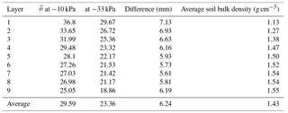
is the average soil moisture content (mm).
The variables saturated hydraulic conductivity (SOL_K) and soil organic carbon content (SOL_CBN), as well as the clay (CLAY), silt (SILT), sand (SAND), and rock fragment (ROCK) contents, were extracted directly from the SLT. The moist soil albedo (SOL_ALB) variable was only required for the top layer as subsequent layers were assigned a value of zero. Since this variable is not reported in the SLC database, it was estimated as the average (i.e., 0.10) of the range reported by Maidment (1993) for moist, dark, plowed fields (i.e., 0.05–0.15). Again, this value was selected since the SLC version 3.2 focuses on agricultural areas, which is also the major domain simulated by SWAT.
Another important variable for SWAT is the erodibility factor (USLE_K), used as an input to the Universal Soil Loss Equation (USLE). This equation is used to calculate soil erosion, which is inherently linked to sediment and nutrient transport (Sharpley et al., 1992, 2002; He et al., 1995; Aksoy and Kavvas, 2005; Koiter et al., 2013) and therefore, critical for simulations of non-point sources of pollution. The erodibility factor was calculated using the method presented by Sharpley and Williams (1990), which is based on the sand, silt, clay, and organic carbon content of the soil (Eq. 1):
where K is the erodibility factor (0.01 ton ac h ac ft-ton in−1), ms is the sand content (%), msilt is the silt content (%), mc is the clay content (%), and orgC is the organic carbon content (%) of the respective soil layer.
As for SOL_ALB, USLE_K is only required for the top layer and subsequent layers were also assigned a value of zero. When converted from imperial to SI units (Foster et al., 1981), the range of calculated values (Table 4) generally agrees with the ranges reported for Canada (Wall et al., 2002), taking into consideration that K values may vary, depending on particle size distribution, organic matter, and structure and permeability of individual soils (Wall et al., 2002). However, the units in the dataset presented here were kept in imperial units for consistency with the SWAT input format. The spatial distribution of the erodibility factor (Fig. 3) was anticipated to align with the HSG, which was the case in areas of low erosion potential in Saskatchewan, where sandy soils prevail, and in areas where runoff potential is high such as in southern Ontario. However, the spatial distribution of USLE_K somewhat contrasted to that of the HSG in some areas of Manitoba and British Columbia, where low sediment transport potential was predicted in areas with high runoff potential. This contrast was likely due to other factors reducing the potential for sediment transport, such as soils with high clay to silt ratios or high organic carbon contents (Sharpley and Williams, 1990).
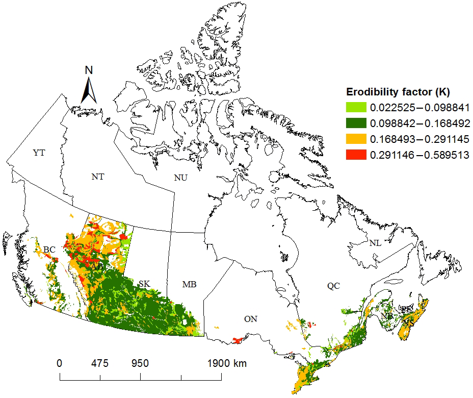
Figure 3Spatial distribution of the erodibility factor (K) calculated for the Soil Landscapes of Canada (SLC) database (imperial units). The K factor shown for the provinces of Prince Edward Island (PE), Nova Scotia (NS), New Brunswick (NB), Quebec (QC), Ontario (ON), Manitoba (MB), Saskatchewan (SK), Alberta (AB), and British Columbia (BC). Some HSGs could not be mapped (e.g., province of Newfoundland and Labrador (NL)) due to missing records in the PAT of the GIS layer or being part of the soils with missing data in the SLT.
Table 4Comparison between the average erodibility factor (K) calculated for each soil textural class in the SWAT dataset and values reported in the literature.
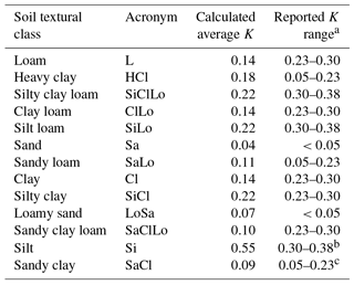
a Adapted from Wall et al. (2002). b Range not reported; value from SiLo used. c Range not reported; value from SaLo used.
The soil electrical conductivity (SOL_EC) information was extracted directly from the SLT. The last 20 columns of the dataset (i.e., columns 133 to 152), which correspond to SOL_CAL for the 10 soil layers followed by SOL_PH for the same layers, were all populated with zeros since these variables are not currently active in SWAT. These variables also had values of zero for all the preexisting soil records in the built-in database in the model.
Soil properties are inherently uncertain due to spatial variability and precision of measurement methods (Lacasse and Nadim, 1996). This uncertainty has direct implications for hydrologic simulations and their interpretation (Beven, 2011). The SWAT model simulations, therefore, are subject to the uncertainty of the soil properties used as input. For example, hydraulic conductivity is highly spatially and temporally variable (Hillel, 1998), and these uncertainties are very difficult to be avoided. The processing applied to the original SLC database in the present analysis did not introduce any further uncertainty to the variables reported by SLC (e.g., saturated hydraulic conductivity). There is, however, some uncertainty relating to estimated and calculated parameters. These uncertainties are discussed in this section, although their quantification is beyond the scope of the present work.
An example of introduced uncertainty is the moist soil albedo in the present dataset (0.10), which is the average of a range reported in the literature (Sect. 6.3). However, any value selected would have some uncertainty associated with it from a modeling standpoint because a single value cannot represent the variability in moist soil albedo as the soil dries up. This is a recognized problem when trying to represent spatially or temporally variable parameters (e.g., soil moisture) using a point measurement or single value in hydrological models (Beven, 2011).
Another example of uncertainty is the HSG calculations, which required a number of assumptions. For example, the shallowest annual depth to water table was unavailable in the SLC and therefore estimated based on the drainage class of each soil record. Also, the assumption of artificial drainage resulted in assignment of dual-class HSGs to the less restrictive one. An assessment of HSG in the USA indicated a standard error of about one HSG (Stewart et al., 2012), suggesting that classifying soils in the neighboring groups is not uncommon and that there is some uncertainty associated with those estimates.
The estimation of erodibility factor (K; Eq. 1) would also be subject to uncertainty. This is illustrated by the range of erodibility factors reported for a single soil textural class (Table 4). This variability can arise for different reasons. One already mentioned is the precision of the method used to determine the textural classes. A second one is the procedure used to calculate K. For example, Neitsch et al. (2005) present an equation that requires a soil structure code used in soil classification with many types and subtypes. Since this soil structure code is note reported in the SLC, an alternative relationship (Eq. 4; Sharpley and Williams, 1990) that does not require the soil structure code was used. This relationship was selected to avoid the added uncertainty from estimating the soil structure code.
Finally, one last variable worthwhile discussing in term of uncertainty is the available water capacity of the soil layers. This variable was estimated as the difference between field capacity and permanent wilting point. The procedure used here to estimate available water content (i.e., the difference between field capacity and permanent wilting point) follows the same procedure used by SWAT (Neitsch et al., 2005) and is described elsewhere in the soil physics literature (Hillel, 1998). Therefore, it would not introduce any further uncertainty. However, using the soil moisture content at −10 kPa to replace records with missing soil moisture content at −33 kPa (Sect. 6.3) would introduce some uncertainty in available water capacity for the replaced records.
Overall, prediction of uncertainty in regional hydrologic modeling and a careful input data discrimination analysis prior to calibration is unavoidable (Faramarzi et al., 2015). Especially in large transboundary river basins where a consistent soil dataset is not available from a single source, a careful uncertainty assessment provides information on data and model quality. Although the authors are unaware of SWAT hydrologic simulations in binational watersheds that use soil datasets from both the USA and Canada, maybe due to lack of large-scale datasets for Canada, it is expected that the model output is subject to the quality and quantity of both datasets. Some aspects contributing to this uncertainty are (i) possible discontinuity in the mapping units (i.e., polygons) between the GIS layers of both datasets, (ii) the soil record being mapped in multicomponent polygons in the GIS coverage (Soil Survey Staff, 1999; Agriculture and Agri-Food Canada, 1998), (iii) differences in soil taxonomy between the USA system (Soil Survey Staff, 1999) and the Canadian system (Agriculture and Agri-Food Canada, 1998) of soil classification, (iv) the methods used to measure/estimate the physicochemical variables, which may differ in accuracy and precision, and (v) the natural variability in the calculation of some variables that cannot be measured (e.g., HSG; Stewart et al., 2012). Given the number of aspects influencing trans-boundary uncertainty and the large spatial scale of both the USA and the dataset discussed here, an assessment of such uncertainty is beyond the scope of the present study. However, this assessment is suggested to quantify the share of errors from these sources in hydrologic model projection in both upstream and downstream tributaries. These are the subjects of our continuing studies.
Although the SWAT database is in a proprietary format (i.e., Microsoft Access), the present soils dataset has been published in a nonproprietary format (i.e., comma-separated values (CSV) file) that can be opened in a variety of software packages. However, the dataset can be easily imported into the SWAT soils database using an automated import routine in Microsoft Access (Fig. 4). This import process consists of opening the SWAT2012 database and using the “Import Text File” tool under the “Import & Link” section of the “External Data” tab to read the CSV file. This action will prompt a window where the user can select the path to where the present dataset is stored and specify how and where the data are stored in the database. The option “Append a copy of the record to the table” should be selected, which activates a drop-down menu from which the usersoil table should be highlighted. Once these options have been processed, an “Import Text Wizard” window will be prompted, where the option “Delimited – Characters such as comma or tab separate each field” should be selected. Processing of this selection will prompt another window where the option “comma” should be automatically selected by the wizard. However, the user should activate the box “First Row Contains Field Names” since the first row of the present dataset contains the variable labels. Confirming the processing of the next windows should finalize the import process, and the data should be ready to be used in SWAT predictions.
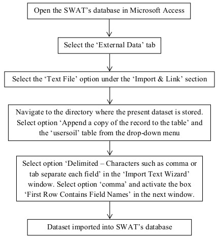
Figure 4Flowchart showing the steps for importing the present soils dataset into SWAT's database.
PANGAEA, an open access library to archive, publish, and distribute georeferenced data, supports database-dependent research. Therefore, the entire dataset (Cordeiro et al., 2017) is published and archived in the PANGAEA database (https://doi.org/10.1594/PANGAEA.877298) under Creative Commons Attribution 3.0 Unported, where the user must give appropriate credit, provide a link to the license, and indicate if changes are made.
The soils dataset presented and discussed in this work represents an effort to facilitate hydrological simulations using the SWAT model in Canada. The dataset consists of a compilation of 11 838 different soil records from the SLC database with all the information required by SWAT and is ready to be imported into the model's soils database. A two-level data screening procedure removed 489 soil records with missing layered information (i.e., not present in the SLT), while 1736 records were removed due to the lack of critical information required by SWAT, such as soil bulk density or saturated hydraulic conductivity. Among the major contributions of this dataset, the calculation and/or estimation of variables not reported in the SLC database are of special importance. The hydrologic soil groups (HSGs) calculated from the SLC database suggest that about half of the soil records in Canada belong to classes with higher potential to generate runoff (i.e., HSG classes 3 and 4). Occurrence of soils in HSG 3 and 4 agree with management practices aimed at addressing excess moisture conditions in agricultural fields, such as subsurface drainage in southern Ontario and Manitoba. The erodibility factor, which is another important variable for SWAT simulations of non-point source pollution, suggests a relationship with runoff potential in portions of southern Ontario and Nova Scotia. However, low erodibility potential, likely driven by high clay to silt ratios or high organic carbon content, was found in areas with higher runoff potential in Manitoba and British Columbia.
The supplement related to this article is available online at: https://doi.org/10.5194/essd-10-1673-2018-supplement.
MRCC and RK developed the concept for development of the dataset. GL interpreted the soil information contained in the SLC database. MRCC and GL developed the methodology for deriving the soil variables. MRCC developed the code using R programming language to process the SLC dataset and performed data analysis. All the authors revised the dataset and participated in manuscript preparation.
The authors declare that they have no conflict of interest.
This research was supported by the Beef Cattle Research Council and Agriculture
and Agri-Food Canada through the Beef Cluster, Environmental Footprint of
Beef Project, and the Alberta Livestock and Meat Agency (ALMA) of the Alberta
Agriculture and Forestry (grant no. 2016E017R).
Edited by: David Carlson
Reviewed by: two
anonymous referees
Agriculture and Agri-Food Canada: The Canadian System of Soil Classification, 3rd Edn., 93, NRC Research Press, Ottawa, 188 pp., 1998.
Ahmad, H. M. N., Sinclair, A., Jamieson, R., Madani, A., Hebb, D., Havard, P., and Yiridoe, E. K.: Modeling sediment and nitrogen export from a rural watershed in eastern Canada using the Soil and Water assessment Tool, J. Environ. Qual., 40, 1182–1194, https://doi.org/10.2134/jeq2010.0530, 2011.
Ahuja, L. R., Andales, A. A., Ma, L., and Saseendran, S. A.: Whole-System Integration and Modeling Essential to Agricultural Science and Technology for the 21st Century, Journal of Crop Improvement, 19, 73–103, https://doi.org/10.1300/J411v19n01_04, 2007.
Aksoy, H. and Kavvas, M. L.: A review of hillslope and watershed scale erosion and sediment transport models, Catena, 64, 247–271, https://doi.org/10.1016/j.catena.2005.08.008, 2005.
Arnold, J., Kiniry, J., Srinivasan, R., Williams, J., Haney, E., and Neitsch, S.: SWAT 2012 Input/Output Documentation, Texas Water Resources Institute, 2013.
Arnold, J. G., Srinivasan, R., Muttiah, R. S., and Williams, J. R.: Large area hydrologic modeling and assessment part i: Model development, J. Am. Water Resour. As., 34, 73–89, https://doi.org/10.1111/j.1752-1688.1998.tb05961.x, 1998.
Arnold, J. G., Moriasi, D. N., Gassman, P. W., Abbaspour, K. C., White, M. J., Srinivasan, R., Santhi, C., Harmel, R. D., Griensven, A. v., Liew, M. W. V., Kannan, N., and Jha, M. K.: SWAT: Model Use, Calibration, and Validation, T. ASABE, 55, 1491–1508, 2012.
Asadzadeh, M., Leon, L., McCrimmon, C., Yang, W., Liu, Y., Wong, I., Fong, P., and Bowen, G.: Watershed derived nutrients for Lake Ontario inflows: Model calibration considering typical land operations in Southern Ontario, J. Great Lakes Res., 41, 1037–1051, https://doi.org/10.1016/j.jglr.2015.09.002, 2015.
Batjes, N. H.: A world dataset of derived soil properties by FAO–UNESCO soil unit for global modelling, Soil Use Manage., 13, 9–16, https://doi.org/10.1111/j.1475-2743.1997.tb00550.x, 1997.
Beven, K. J.: Rainfall-Runoff Modelling: The Primer, Wiley, West Sussex, UK, 2011.
Bossa, A. Y., Diekkrüger, B., Igué, A. M., and Gaiser, T.: Analyzing the effects of different soil databases on modeling of hydrological processes and sediment yield in Benin (West Africa), Geoderma, 173–174, 61–74, https://doi.org/10.1016/j.geoderma.2012.01.012, 2012.
Bower, S. S.: Watersheds: Conceptualizing Manitoba's drained landscape, 1895–1950, Environ. Hist., 12, 796–819, https://doi.org/10.1093/envhis/12.4.796, 2007.
Bronswijk, J. J. B.: Prediction of actual cracking and subsidence in clay soils, Soil Sci., 148, 87–93, 1989.
Chambers, P. A., Benoy, G. A., Brua, R. B., and Culp, J. M.: Application of nitrogen and phosphorus criteria for streams in agricultural landscapes, Water Sci. Technol., 64, 2185–2191, https://doi.org/10.2166/wst.2011.760, 2011.
Cooper, M., Mendes, L. M. S., Silva, W. L. C., and Sparovek, G.: A National Soil Profile Database for Brazil Available to International Scientists, Soil Sci. Soc. Am. J., 69, 649–652, https://doi.org/10.2136/sssaj2004.0140, 2005.
Cordeiro, M. R. C. and Sri Ranjan, R.: Corn yield response to drainage and subirrigation in the Canadian Prairies, Transactions of the American Society of Agricultural Engineers, 55, 1771–1780, https://doi.org/10.13031/2013.42369, 2012.
Cordeiro, M. R. C. and Sri Ranjan, R.: DRAINMOD simulation of corn yield under different tile drain spacing in the Canadian Prairies, Transactions of the American Society of Agricultural Engineers, 58, 1481–1491, https://doi.org/10.13031/trans.58.10768, 2015.
Cordeiro, M. R. C., Lelyk, G., Kröbel, R., Legesse, G., Faramarzi, M., Masud, M. B., and McAllister, T.: Deriving Canada-wide soils dataset for use in Soil and Water Assessment Tool (SWAT), PANGAEA, https://doi.org/10.1594/PANGAEA.877298, 2017.
Dobos, E., Daroussin, J., and Montanarella, L.: An SRTM-based procedure to delineate SOTER Terrain Units on 1 : 1 and 1 : 5 million scales. EUR 21571 EN, Office for Official Publications of the European Communities, Luxembourg, 2005.
Douglas-Mankin, K. R., Srinivasan, R., and Arnold, J. G.: Soil and Water Assessment Tool (SWAT) Model, Current Developments and Applications, 53, 1423–1431, https://doi.org/10.13031/2013.34915, 2010.
Edwards, L., Burney, J., Brimacombe, M., and Macrae, A.: Nitrogen runoff in a potato-dominated watershed area of Prince Edward Island, Canada, The Role of Erosion and Sediment Transport in Nutrient and Contaminant Transfer, Waterloo, ON, 93–97, 2000.
Faramarzi, M., Srinivasan, R., Iravani, M., Bladon, K. D., Abbaspour, K. C., Zehnder, A. J. B., and Goss, G. G.: Setting up a hydrological model of Alberta: Data discrimination analyses prior to calibration, Environ. Modell. Softw., 74, 48–65, https://doi.org/10.1016/j.envsoft.2015.09.006, 2015.
Foster, G. R., McCool, D. K., Renard, K. G., and Moldenhauer, W. C.: Conversion of the universal soil loss equation, J. Soil Water Conserv., 36, 355–359, 1981.
Gao, G. Y., Fu, B. J., Lü, Y. H., Liu, Y., Wang, S., and Zhou, J.: Coupling the modified SCS-CN and RUSLE models to simulate hydrological effects of restoring vegetation in the Loess Plateau of China, Hydrol. Earth Syst. Sci., 16, 2347–2364, https://doi.org/10.5194/hess-16-2347-2012, 2012.
Gassman, P. W., Sadeghi, A. M., and Srinivasan, R.: Applications of the SWAT model special section: Overview and insights, J. Environ. Qual., 43, 1–8, https://doi.org/10.2134/jeq2013.11.0466, 2014.
Givi, J., Prasher, S. O., and Patel, R. M.: Evaluation of pedotransfer functions in predicting the soil water contents at field capacity and wilting point, Agr. Water Manage., 70, 83–96, https://doi.org/10.1016/j.agwat.2004.06.009, 2004.
He, Z. L., Wilson, M. J., Campbell, C. O., Edwards, A. C., and Chapman, S. J.: Distribution of phosphorus in soil aggregate fractions and its significance with regard to phosphorus transport in agricultural runoff, Water Air Soil Poll., 83, 69–84, https://doi.org/10.1007/bf00482594, 1995.
Hillel, D.: Environmental Soil Physics: Fundamentals, Applications, and Environmental Considerations, Elsevier Science, London, UK, 1998.
Koiter, A. J., Lobb, D. A., Owens, P. N., Petticrew, E. L., Tiessen, K. H. D., and Li, S.: Investigating the role of connectivity and scale in assessing the sources of sediment in an agricultural watershed in the Canadian prairies using sediment source fingerprinting, J. Soils Sediment., 13, 1676–1691, https://doi.org/10.1007/s11368-013-0762-7, 2013.
Lacasse, S. and Nadim, F.: Uncertainties in characterising soil properties, Uncertainty in the geologic environment: From theory to practice, 49–75, 1996.
Laniak, G. F., Olchin, G., Goodall, J., Voinov, A., Hill, M., Glynn, P., Whelan, G., Geller, G., Quinn, N., Blind, M., Peckham, S., Reaney, S., Gaber, N., Kennedy, R., and Hughes, A.: Integrated environmental modeling: A vision and roadmap for the future, Environ. Model. Softw., 39, 3–23, https://doi.org/10.1016/j.envsoft.2012.09.006, 2013.
Lévsque, É., Anctil, F., Van Griensven, A. V., and Beauchamp, N.: Evaluation of streamflow simulation by SWAT model for two small watersheds under snowmelt and rainfall, Hydrolog. Sci. J., 53, 961–976, https://doi.org/10.1623/hysj.53.5.961, 2008.
Maidment, D. R.: Handbook of hydrology, McGraw-Hill, New York, 1993.
Mapfumo, E., Chanasyk, D. S., and Willms, W. D.: Simulating daily soil water under foothills fescue grazing with the soil and water assessment tool model (Alberta, Canada), Hydrol. Process., 18, 2787–2800, https://doi.org/10.1002/hyp.1493, 2004.
Mednick, A. C.: Comparing the use of STATSGO and SSURGO soils data in water quality modeling: A literature review, Bureau of Science Services, Wisconsin Department of Natural Resources, 2008.
Mekonnen, B. A., Mazurek, K. A., and Putz, G.: Incorporating landscape depression heterogeneity into the Soil and Water Assessment Tool (SWAT) using a probability distribution, Hydrol. Process., 30, 2373–2389, https://doi.org/10.1002/hyp.10800, 2016.
Moeys, J.: soiltexture: Functions for Soil Texture Plot, Classification and Transformation. R package version 1.4.1, available at: https://CRAN.R-project.org/package=soiltexture (last access: 1 June 2017), 2016.
Moriasi, D. N. and Starks, P. J.: Effects of the resolution of soil dataset and precipitation dataset on SWAT2005 streamflow calibration parameters and simulation accuracy, J. Soil Water Conserv., 65, 63–78, https://doi.org/10.2489/jswc.65.2.63, 2010.
Neitsch, S., Arnold, J., Kiniry, J., Williams, J., and King, K.: SWAT2009 Theoretical Documentation, Texas Water Ressources Institute Technical Report, 2005.
Rahman, M., Bolisetti, T., and Balachandar, R.: Hydrologic modelling to assess the climate change impacts in a Southern Ontario watershed, Can. J. Civil Eng., 39, 91–103, https://doi.org/10.1139/l11-112, 2012.
Rasouli, S., Whalen, J. K., and Madramootoo, C. A.: Review: Reducing residual soil nitrogen losses from agroecosystems for surface water protection in Quebec and Ontario, Canada: Best management practices, policies and perspectives, Can. J. Soil Sci., 94, 109–127, https://doi.org/10.4141/cjss2013-015, 2014.
Santhi, C., Muttiah, R. S., Arnold, J. G., and Srinivasan, R.: A gis-based regional planning tool for irrigation demand assessment and savings using SWAT, Transactions of the American Society of Agricultural Engineers, 48, 137–147, https://doi.org/10.13031/2013.17957, 2005.
Sharpley, A. N. and Williams, J. R.: EPIC-erosion/productivity impact calculator: 1. Model documentation, Technical Bulletin-United States Department of Agriculture, Washington DC, 1990.
Sharpley, A. N., Smith, S. J., Jones, O. R., Berg, W. A., and Coleman, G. A.: The transport of bioavailable phosphorus in agricultural runoff, J. Environ. Qual., 21, 30–35, https://doi.org/10.2134/jeq1992.00472425002100010003x, 1992.
Sharpley, A. N., Kleinman, P. J. A., McDowell, R. W., Gitau, M., and Bryant, R. B.: Modeling phosphorus transport in agricultural watersheds: Processes and possibilities, J. Soil Water Conserv., 57, 425–439, 2002.
Sheshukov, A., Daggupati, P., Lee, M.-C., and Douglas-Mankin, K.: ArcMap tool for pre-processing SSURGO soil database for ArcSWAT, 5th SWAT International Conference, Boulder, CO, 2009.
Shi, X. Z., Yu, D. S., Warner, E. D., Pan, X. Z., Petersen, G. W., Gong, Z. G., and Weindorf, D. C.: Soil Database of 1 : 1,000,000 Digital Soil Survey and Reference System of the Chinese Genetic Soil Classification System, Soil Horizons, 45, 129–136, https://doi.org/10.2136/sh2004.4.0129, 2004.
Soil Landscapes of Canada Working Group: Soil landscapes of Canada version 3.2, Agriculture and Agri-Food Canada (digital map and database at 1 : 1 million scale), Ottawa, ON, Canada, 2010.
Soil Survey Staff: Soil Taxonomy: A basic system of soil classification for making and interpreting soil surveys, Agricultural Handbook 436, Soil Use and management, 1, Natural Resources Conservation Service, 57–60, 1999.
Srinivasan, R., Zhang, X., and Arnold, J.: SWAT ungauged: hydrological budget and crop yield predictions in the Upper Mississippi River Basin, Transactions of the American Society of Agricultural Engineers, 53, 1533–1546, 2010.
Stewart, D., Canfield, E., and Hawkins, R.: Curve number determination methods and uncertainty in hydrologic soil groups from semiarid watershed data, J. Hydrol. Eng., 17, 1180–1187, https://doi.org/10.1061/(ASCE)HE.1943-5584.0000452, 2012.
Stonehouse, D. P.: Profitability of soil and water conservation in Canada: A review, J. Soil Water Conserv., 50, 215–219, 1995.
USDA-NRCS: Hydrologic Soil Groups, in: National Engineering Handbook, Part 630, U.S. Department of Agriculture, Soil Conservation Service, 7.1-7.5, 1993.
Wall, G. J., Coote, D. R., Pringle, E. A., and Shelton, I. J.: Revised Universal Soil Loss Equation for Application in Canada: A Handbook for Estimating Soil Loss from Water Erosion in Canada, Agriculture and Agri-Food Canada, Ottawa, Canada, 2002.
Watson, B. M. and Putz, G.: Comparison of temperature-index snowmelt models for use within an operational water quality model, J. Environ. Qual., 43, 199–207, https://doi.org/10.2134/jeq2011.0369, 2014.
Whittaker, G., Confesor, R., Di Luzio, M., and Arnold, J.: Detection of overparameterization and overfitting in an automatic calibration of SWAT, Transactions of the American Society of Agricultural Engineers, 53, 1487–1499, 2010.
Wolfe, S. A.: Impact of increased aridity on sand dune activity in the Canadian Prairies, J. Arid Environ., 36, 421–432, https://doi.org/10.1006/jare.1996.0236, 1997.
Wösten, J. H. M., Lilly, A., Nemes, A., and Le Bas, C.: Development and use of a database of hydraulic properties of European soils, Geoderma, 90, 169–185, https://doi.org/10.1016/S0016-7061(98)00132-3, 1999.
Yang, Q., Meng, F.-R., Zhao, Z., Chow, T. L., Benoy, G., Rees, H. W., and Bourque, C. P. A.: Assessing the impacts of flow diversion terraces on stream water and sediment yields at a watershed level using SWAT model, Agr. Ecosyst. Environ., 132, 23–31, https://doi.org/10.1016/j.agee.2009.02.012, 2009.
Yang, Q., Leon, L. F., Booty, W. G., Wong, I. W., McCrimmon, C., Fong, P., Michiels, P., Vanrobaeys, J., and Benoy, G.: Land use change impacts on water quality in three Lake Winnipeg watersheds, J. Environ. Qual., 43, 1690–1701, https://doi.org/10.2134/jeq2013.06.0234, 2014.
Zhu, Z., Broersma, K., and Mazumder, A.: Impacts of land use, fertilizer and manure application on the stream nutrient loadings in the Salmon River watershed, south-central British Columbia, Canada, J. Environ. Prot., 3, 14, https://doi.org/10.4236/jep.2012.328096, 2012.
- Abstract
- Introduction
- SLC data structure
- SWAT soils data structure
- Merging the two datasets
- Data screening
- Populating the usersoil table in SWAT
- Uncertainty
- Importing the SLC dataset into the SWAT database
- Data availability
- Conclusions
- Author contributions
- Competing interests
- Acknowledgements
- References
- Supplement