UDASH – Unified Database for Arctic and Subarctic Hydrography

UDASH (Unified Database for Arctic and Subarctic Hydrography) is a unified and high-quality temperature and salinity data set for the Arctic Ocean and the subpolar seas north of 65^∘ N for the period 1980–2015. The archive aims at including all publicly available data and so far consists of 288 532 oceanographic profiles measured mainly with conductivity–temperature–depth (CTD) probes, bottles, mechanical thermographs and expendable thermographs. The data were collected by ships, ice-tethered profilers, profiling floats and other platforms. To achieve a uniform quality level, suitable for a wide range of oceanographic analyses, approximately 74 million single measurements of temperature and salinity were thoroughly quality checked. A large number of duplicate and erroneous profiles were detected and not included in the archive. Data outliers were flagged for quick identification. The final archive provides a unique and simple way of accessing most of the available temperature and salinity data for the Arctic Ocean and can be downloaded from https://doi.pangaea.de/10.1594/PANGAEA.872931.

1 Introduction

With the increasing awareness of global climate change, the Arctic receives much attention as it undergoes rapid changes in the atmosphere, sea ice, glaciers, ice sheets, snow and permafrost (e.g., Comiso and Hall, 2014; Boisvert and Stroeve, 2015). This has widespread impacts on Arctic communities and ecosystems (e.g., Wassmann et al., 2011; Wrona et al., 2016). The Arctic Ocean covers much of the polar region and is a strong focus of these changes. A prominent example is that increasing amounts of freshwater from melting ice and continental runoff can affect deep water formation and, in turn, the strength of the Atlantic meridional overturning circulation (e.g., Curry and Mauritzen, 2005; Yang et al., 2016). On the other hand, warm water pulses, intruding the Arctic Ocean from lower latitudes, may affect the local climate and sea ice system (e.g., Shimada et al., 2006; Polyakov et al., 2010; Beitsch et al., 2014). Studying the Arctic Ocean has thus become an integral part of modern Earth system science.

The extensive sea ice cover limits the access to the Arctic Ocean throughout much of the year. Oceanographic data in high latitudes are therefore sparse in both space and time. In the recent years, however, highly developed measurement techniques were especially designed for operation in the Arctic environment (e.g., Toole et al., 2011). Furthermore, an increasing number of research activities and international collaboration – such as the International Polar Year (IPY) (Mauritzen et al., 2011) – has generated a large number of hydrographic data in the central Arctic and the subarctic seas (e.g., Rabe et al., 2014). Most of these data are publicly available from different online archives. However, they sometimes contain redundant profiles and data of different quality. Moreover, oceanographic data from the various archives often have undergone different kinds of quality-testing procedures. To date, none of these archives offers a complete collection of all available temperature and salinity measurements in the Arctic Ocean with a uniform quality level.

We therefore have compiled a comprehensive hydrographic database (UDASH, Unified Database for Arctic and Subarctic Hydrography) of the Arctic Ocean, which can be used for oceanographic studies and data assimilation. We aimed at compiling a database that meets the following requirements: the database

1. contains all publicly available data for a certain time period,

2. can be used without extensive quality testing,

3. is easily accessible,

4. well documented and

5. open for updates.

A long-term goal is to use the quality-controlled data to produce an updated Arctic Ocean climatology as a reference for ocean models. A widely used climatology for models is the Polar Science Center Hydrographic Climatology (PHC) (Steele et al., 2001), which includes data mainly up to the 1990s.

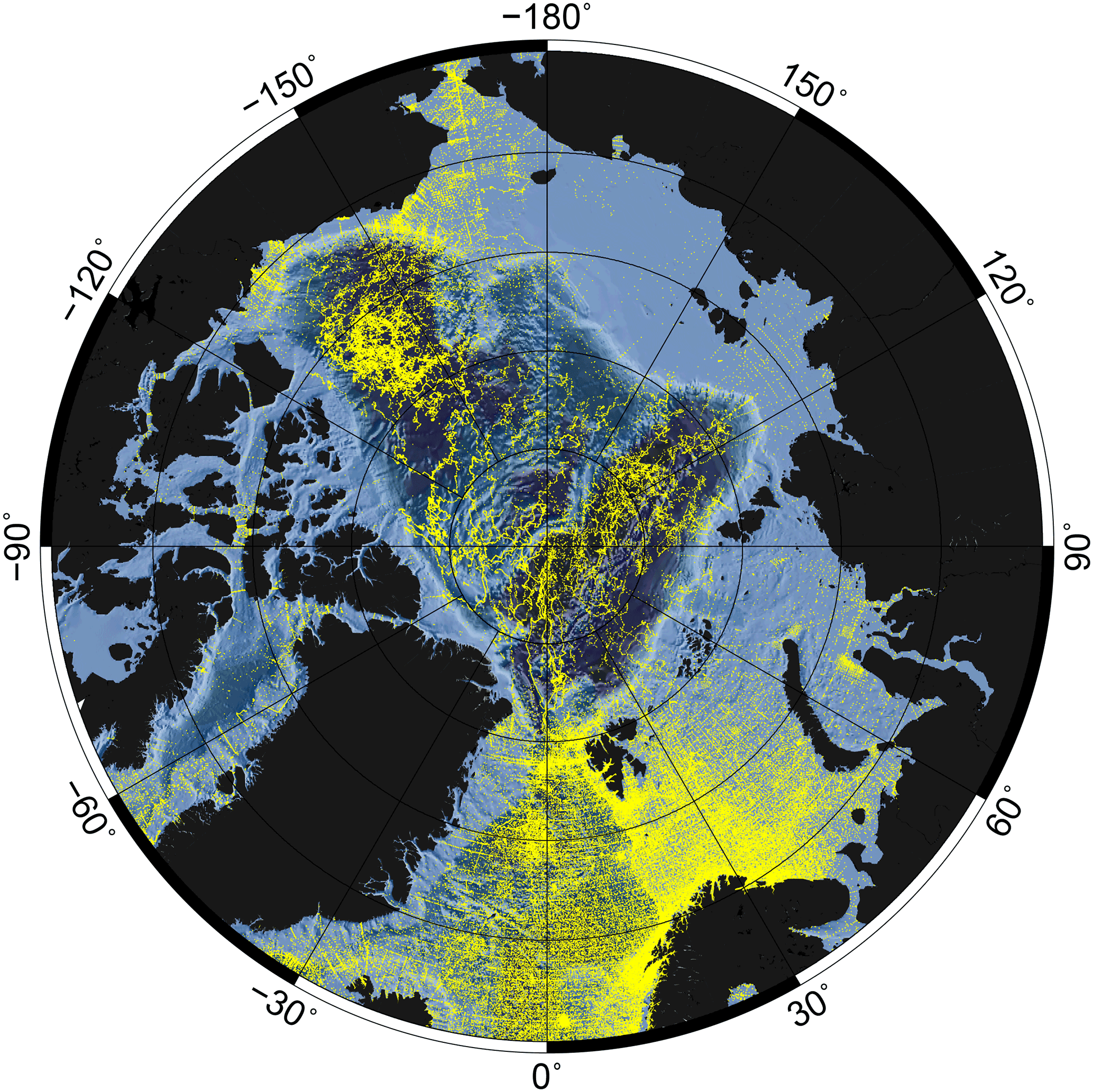
Figure 1 Data coverage after quality check and data validation. Size: 288 532 profiles. Period: 1980–2015. Region: north of 65^∘ N.

The paper is organized as follows. Section 2 gives an overview on the different data sources. Section 3 contains detailed descriptions of the quality checks (QC), the changes applied to some of the data and the flagging system. Section 4 presents a detailed overview on the final data set with distribution maps, statistics and diagrams. Section 5 contains information on the data availability. A short summary and outlook is given in Sect. 6. The numbers and statistics provided in the following sections represent the status of the data archive at the time of publication. They will change, as the archive will be updated in the near future.

2 Data

2.1 Data coverage

The data set covers the full Arctic Ocean north of 65^∘ N (Fig. 1) and spans the period 1980–2015. We selected 1980 as the starting point, because the available data before the mid-1980s are mainly confined to the shelf regions and the subarctic seas and do not cover the deep basins of the central Arctic Ocean. Furthermore, the time frame of 36 years may in some regions (e.g., Barents Sea) enable investigations over climatically relevant time periods. There is the possibility of future updates with data prior to 1980.

2.2 Data from the World Ocean Database

The largest public archive for hydrographic data is the World Ocean Database (WOD) (Boyer et al., 2013) of the US National Oceanic and Atmospheric Administration (NOAA). WOD includes many Arctic data, dating back to the mid-1800s (Zweng et al., 2017). Oceanic profiles from the 2013 version (wod13) of this source constitute 76.6 % (221 117 profiles) of our quality-checked data set. WOD data are already quality checked, and we used WOD quality flags during our QC procedures. We found, however, that the accepted values still contain a significant number of outliers and biases (see Sect. 4). Moreover, wod13 does not contain all available data for our period, e.g., data from RV Polarstern (Driemel et al., 2017).

Table 1 Data sources and their abbreviations used in the data files. Also shown are time periods and URLs of the downloaded data.

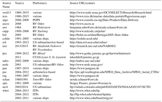
Table 2 Format of the variables and metadata in different columns of the data files.

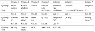
Platform abbreviations. S: ships, I: ice tethered, A: helicopters/airplanes, F: profiling floats, SU: submarines, C: ice camps, CO: coastal station, NA: unknown.
Instrument abbreviations. CTD: conductivity–temperature–depth, XCTD: expendable CTD, B: bottle, STD: salinity–temperature–depth, XBT: expendable bathythermograph, MBT: mechanical bathythermograph, DBT: digital bathythermograph.

The downloaded wod13 data include measurements from the following platforms and instrument types (acronyms used by WOD are shown in brackets): ship-borne conductivity–temperature–depth (CTD, high and low vertical resolution), expendable CTD (XCTD), drifting buoys (DRB), profiling floats (PFL), expendable bathythermographs (XBT), digital bathythermographs (DBT), salinity–temperature–depth measurements (STD), mechanical bathythermographs (MBT) and bottle data (B). For XBT depth bias correction, we selected the Gouretski (2012) method. When downloading data from WOD, the correction is automatically applied to the selected profiles. Glider data were neglected, as these data are restricted to only a few regions at the southern boundary of the domain. Our QC routines (see next section) are, furthermore, designed for testing oceanographic profiles that were measured in a fixed position. Our current data set therefore does not include mooring data. They will be included in a forthcoming update.

2.3 Data from other sources

The WOD data were supplemented with measurements from other sources (Table 1). This resulted in an additional number of 67 415 profiles (after quality check), which increased the data density also in the central Arctic. The final archive includes data from the following platforms: ships, submarines, profiling floats, ice-tethered platforms (ITPs) (such as Polar Ocean Profiling Systems, POPS), helicopter/aircraft, drifting ice camps and one coastal station (see Table 2 for abbreviations). We are aware that there may be other sources which we have not included so far. They can be considered in a future update of the archive.

2.4 Data format

The data files are provided in a 19-column ASCII format, with one file for each year (36 in total). The format can be easily imported to Ocean Data View (Schlitzer, 2002). In total, the files include approximately 74 million lines (single measurements), forming 288 532 stacked profiles of temperature and salinity. For example, one CTD profile with a vertical resolution of 1 m and a maximum depth of 1200 m would form a matrix with dimensions (1200 × 19).

The data structure is listed in Table 2. Column 1 contains the profile number (between 1 and 288 532). The cruise and/or platform identification is stored in column 2. For wod13 data, we stored the name of the platform or the originator's cruise identification. If both were available, we combined them to ensure a good traceability of the data. For data from sources other than wod13 we also stored as much information as possible. Column 3 contains the station number that belongs to the respective profile. In column 4 and 5 the platform type and instrument type is stored, respectively. Column 6 contains the timestamp, and columns 7 and 8 contain the geographical longitude and latitude, respectively. The oceanographic parameters are pressure (column 9), depth (column 10), in situ temperature (column 12) and salinity (column 14). Depth was converted to pressure by using the TEOS-10 Gibbs SeaWater library (IOC et al., 2010). Quality flags were assigned to pressure and depth (column 11), temperature (column 13) and salinity (column 15) according to the tests described in the next section. Column 16 contains the source from which the data were obtained (Table 1) and column 17 the digital object identifier (DOI). The DOI information is not yet complete and will be updated in the future. Columns 18 and 19 contain the WOD unique cruise and cast identifications, respectively, to ensure good traceability of the individual profiles. These columns are empty for data sources other than wod13. Cells with no information contain the value −999. Some profiles were available only with date information. In this case the missing time information is coded as 99:99 (e.g., 2011-08-24T99:99).

Most of the data have undergone different kinds of quality tests applied by the respective data providers. To remove all duplicate profiles and to guarantee a uniform data quality, we applied additional tests.

3 Quality checks

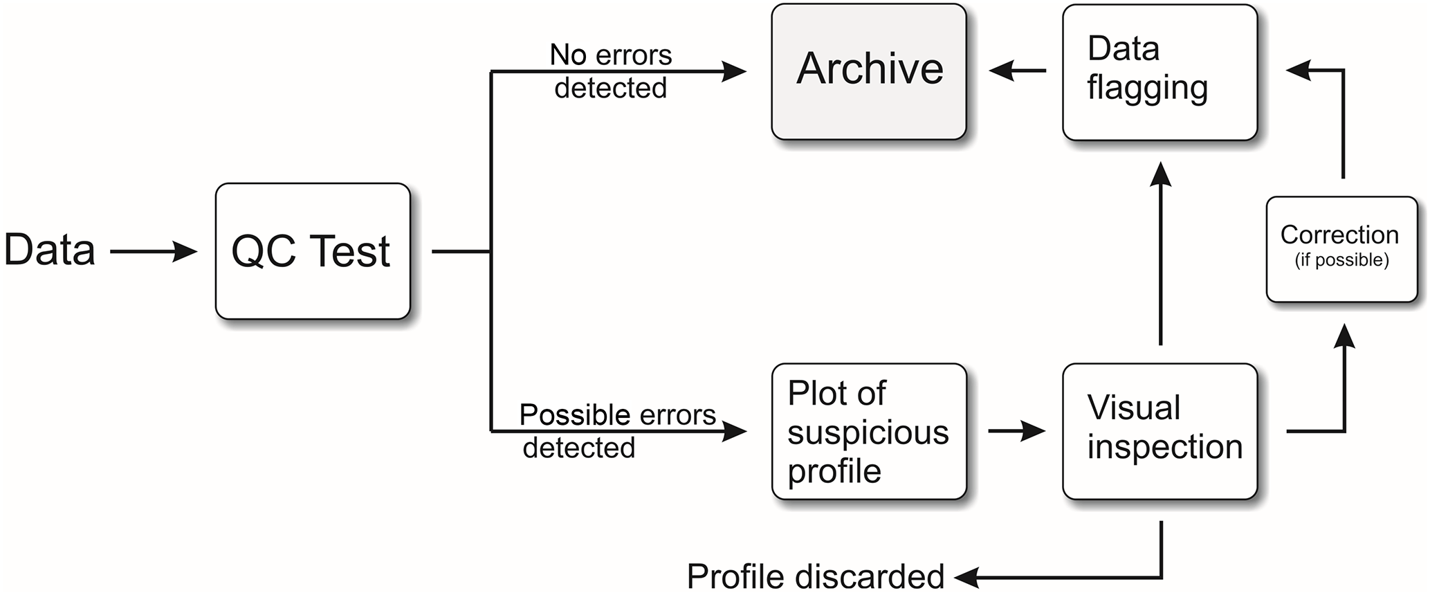
Several procedures have been developed to detect and eliminate errors in hydrographic profiles (e.g., Ingleby and Huddleston, 2007; Gronell and Wijffels, 2008; Manzella and Gambetta, 2013). When applied to global oceanographic databases, these procedures often rely on fully automatic tests, as the large number of data precludes the detailed visual assessment of individual profiles by experienced data scientists. These automated procedures are highly developed and efficiently remove erroneous data from large oceanographic archives. A problem is, however, that efficient detection algorithms always falsely eliminate a certain amount of good data, which can reduce the size of quality-checked data sets significantly. This may be feasible in regions with high data density (e.g., the North Atlantic), but is not acceptable in high latitudes where the data density is low. Some QC tests for temperature and salinity profiles are therefore semiautomated procedures that also include visual inspection of detected errors by data analysts (e.g., Gronell and Wijffels, 2008). Another problem with fully automatic tests is that they may reduce the natural variability of the measured quantities. A common method for automatically eliminating unrealistic values is to plot the profiles for a certain domain and to delete all values that are higher (lower) than the mean plus (minus) a threshold value, usually a multiple of the standard deviation. Determining this threshold value is a difficult task, as one aims to eliminate wrong data and at the same time tries to keep the real variability or trends in the data unaffected. When correcting the data in this way, it is also not possible to detect profiles that are weakly biased or profiles with position errors.

For the above reasons, our QC procedures mainly include semiautomatic tests. The principle is outlined in Fig. 2. It is based on visual assessment of all profiles that did not pass a certain quality test. These profiles then either directly enter the final archive, or are discarded or flagged for further treatment.

We started with 122 565 176 single measurements (lines), forming 467 991 oceanographic profiles of temperature and salinity. Each profile was assigned an identification (ID) number to enable good traceability and quick access during the QC process. The testing routine applied to our data set can be divided into four steps: duplication checks, position checks, gradient checks and statistical screening.

Figure 2 Working principle of the data-quality testing.

3.1 Step one: duplication checks

Ship-borne CTD measurements and bottle data are typically recorded at the same cast. We therefore first excluded all bottle data, when a CTD measurement was taken at the same time and at the same position. Next, we use the method of Gronell and Wijffels (2008) to detect and exclude exact duplicates. These profiles are detected by comparing the number of depths, the sum of depths and the sum of temperatures. If identical profiles had different timestamps (> 2 days), both were excluded, if not, only one was excluded.

In the next step so-called near duplicates are detected. Near duplicates are profiles measured at (almost) the same time and position and that show small differences in the temperature and depth values. This includes profile pairs that were interpolated to different vertical resolutions, pairs that extend to different depths or pairs that contain different numbers of outliers. The algorithm also detects groups of near duplicates when similar profiles are present in more than two sources. Near duplicates are detected by first finding all profiles within ±0.1^∘ in latitude and longitude around each position (Gronell and Wijffels, 2008). We also allowed for an uncertainty in the timestamp of ≤ 5 h. We used this value because most of the ITP profiles were recorded 6 h apart. They are therefore often very close in space, but should not be detected as near duplicates. Whenever a time difference of 1 day was detected, we additionally checked the source. If the source was wod13, we excluded this profile, because when comparing ITP data from the sources whoi and wod13 (Table 1) we found that in many cases the timestamps of the same profiles show a difference of exactly 24 h. All profiles within the search windows in time and space were then truncated to the depth range they have in common and then interpolated to the same vertical grid. If 75 % of their temperatures matched, they were considered identical. We rounded the temperatures to one decimal place to mimic changes that may occur when data migrate through different computer systems (Gronell and Wijffels, 2008).

We always retained the profiles with the largest amount of information and excluded, for example, all truncated near duplicates. When exact duplicates or near duplicates were found in different sources, we preferred the data from the primary source to avoid errors that occur during data conversion for the import into a database.

The duplicate and near-duplicate checks are fully automatic, but we visually inspected sample profiles to validate the tests. Duplicate profiles found during both tests were excluded from the archive. In total we excluded 12 592 profiles from identical pairs or groups and 69 204 profiles from nearly identical pairs or groups.

The duplication checks also revealed inconsistencies in the instrument types between different data sources. In some cases the same profile was labeled with B (bottle) in the ICES archive and with CTD in WOD. Furthermore, we detected some uncertainties in ship names, i.e., the same profile measured by different ships. This indicates that an unknown degree of uncertainty exists in the metadata.

Figure 3 Sample output of the cruise-track test. (a) Cruise track in the southern Barents Sea. Source: wod13. Cruise ID: SU-8114 (bottle data). Position 28 (red circle) represents a cruise-track outlier. Date of wrong position: 7 January 1989. (b) Cruise track in the southern Beaufort Sea. Source: wod13. Cruise/ship: ARCTIC_IVIK. Cruise ID: CA-12540 (bottle data). Position 13 (red circle) has a wrong timestamp. Date of wrong position: 12 September 1986.

3.2 Step two: position checks

This step aims at identifying profiles with incorrect geographical position. These errors sometimes occur during the initial processing of raw data or when they are imported into databases. We applied two steps to detect position errors. In the first step we calculated the ocean depth at the considered profile position. The depth was interpolated from the international bathymetric chart of the Arctic Ocean (IBCAO version 3.0) (Jakobsson et al., 2012) by using the neighboring grid points of the profile position. We assumed an interpolation error of 200 m and looked for profiles in which the depth of the deepest measurement was located more than 200 m below the ocean bottom. The suspicious profiles were plotted and excluded if the position was considered unrealistic. This step also identifies profiles that were located on land. In this case the interpolated ocean depth is negative. As the IBCAO bathymetry is inaccurate in some regions, a very careful inspection of the possible position errors was necessary. For some recent cruises with definitely correct positions, single measurements were located up to 1000 m below the seafloor on the continental slope (e.g., in the Laptev Sea). We therefore did not exclude profiles with detected position errors above continental slopes in regions with strongly rugged seafloor and sometimes also near coastlines. Automatically excluded in this test were only those profiles that were located in a shelf sea and in which the deepest measurement was found deeper than 500 m. For the Barents Sea the threshold was set to 800 m depth.

In the second step the cruise-track check (Ingleby and Huddleston, 2007) was applied. The test is based on calculating speeds of ships or drifting buoys, traveled distances and angles between different positions. In this way it detects excessive velocities, kinks in the cruise track and looks for other suspicious distance–time relationships. The track check also enables the detection of wrong positions which are not picked by the test described above. Single cruises were identified by their cruise or platform name, the data source and – for data from wod13 – the NODC (National Oceanographic Data Center) cruise ID. The profiles of a cruise were ordered by time and again split into different cruises, when the stations were separated by time periods of more than 30 days. For some data, only an NODC cruise ID and no platform or cruise name was available. These cases were treated with special care, as the data could originate from different platforms operating at the same time. The test was skipped for WOD data when neither an NODC cruise number nor a platform or cruise name was given. It was also skipped for airplane and helicopter missions, as the track check includes maximum speed thresholds only for ships (15 m s⁻¹) and drifting buoys (2 m s⁻¹) (Ingleby and Huddleston, 2007). We included a speed threshold for ITPs, POPS and drifting ice camps of 1 m s⁻¹. The test was not applied to cruises with platform names such as ROYAL_NAVY_NON-SURVEY_VESSELS (e.g., profile number 283 669) and MULTIPLE_SHIPS (e.g., profile number 68 905).

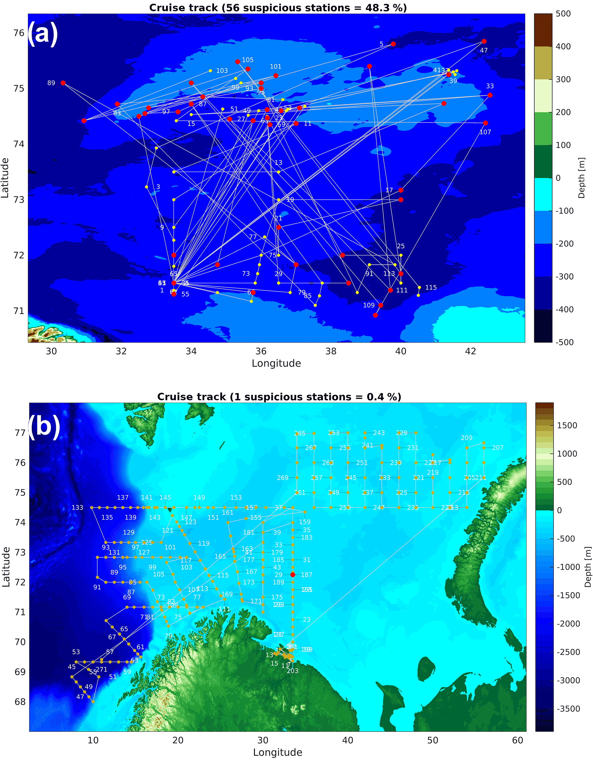
Figure 4 Sample output of the cruise-track test. (a) Cruise track in the Barents Sea (August 1988) with possible position errors and errors in the timestamps. Source: wod13. Cruise ID: SU-89247 (MBT data). (b) Cruise track in the Barents Sea (July 1989). Source: wod13. Cruise: MI0847. Cruise ID: RU-118 (bottle data).

The cruise-track test is also able to detect errors in the timestamp. In this case, the cruise track shows sudden jumps from one section to another and back (Fig. 3b). These profiles were only excluded in regions with high data density (e.g., Barents and Nordic Seas). In the central Arctic the profiles were flagged and not excluded, when the time error was considered small (e.g., less than 1 day). In some cases we excluded whole cruises from the archive, when the cruise identification was successful but the cruise track showed a chaotic pattern (Fig. 4a) with more than 30 % position outliers and obvious errors in the timestamps. However, one has to be aware that not all data were obtained from scientific cruises and show the typical patterns with oceanographic sections (Fig. 4b). Many early data in the Barents and Nordic Seas were recorded by fishing vessels, especially during the Soviet era. A common error detected by the track check is the sign error of the longitude value. In most cases only single positions of a cruise had a wrong sign. In one case, however, we found that a whole cruise was located on the wrong side of the prime meridian (source: wod13).

Profiles with obviously wrong positions were excluded from the data, as there is no possibility to correct these in a reliable way. Profiles that failed a position test, but could not be confirmed by visual inspection to be in a wrong position, were flagged (see Sect. 3.6). Position errors that were not detected by the two tests could at times be detected during the statistical parameter screening described below, as the background hydrography differs from region to region.

For the position tests a large number of cruise tracks and single positions had to be assessed visually, as the algorithms have a certain failure rate. In total we excluded 381 profiles found on land, 498 profiles with apparently wrong position (based on the IBCAO bathymetry test) and 360 profiles representing cruise-track outliers.

A total of 69 040 profiles were excluded, because they belonged to cruises that showed a strongly flawed cruise track. The majority of the profiles excluded in this way belong to B and MBT (see Table 1 for acronyms) measurements from the source wod13 in the Barents and Nordic Seas in the 1980s. Most of the excluded profiles from the central Arctic basins seem to originate from drifting platforms. Because of the large amount of data excluded in this way, we decided to reassess some of the cruises in a future update of the archive.

3.3 Step three: gradient checks

In the first step of the gradient check we detected profiles containing multiple measurements on single depth levels. We stored the respective profile ID numbers for the correction applied at the end (see Sect. 3.5). The following main part of the gradient check includes (1) spike and outlier checks, (2) detection of suspicious vertical gradients and (3) a density inversion (stability) check.

All outliers detected by the various algorithms were plotted and visually confirmed (flagged) or rejected (not flagged) if necessary. Some outliers could not be identified in this step, but were detected by one of the tests below. The outlier detection was therefore facilitated by the stability checks and the gradient checks, and also by the statistical screening (see step 4). In the following, we applied tests with different sensitivity for the mixed layer (upper 100 m) and the depths below. This was necessary, as we obtained a very large number of plots with false detections in the upper 100 m, where the high variability can create strong gradients and sometimes density inversions in the mixed layer that are usually not suspicious.

First, we detected bottom and top outliers, i.e., unrealistic values at the very beginning or end of a profile. We defined threshold values: −2 and 15^∘ C for temperature and 10 and 38 (depth < 30 m) and 25 and 38 (depth ≥ 30 m) for salinity. This test was designed to detect single-point spikes and outliers that are formed by more than just one value. Bottom and top outliers were excluded from the data after detailed visual assessment. For example, in some regions, such as fjords or estuaries, salinity values < 10 in the surface layer were not considered unrealistic.

Figure 5 CTD temperature profile measured on 13 July 1998 near the Lofoten Islands. Source: ices. Ship: Johan Hjort. Station: 434. Two outliers (red dots) were detected at around 400 m depth (artificially induced) and 800 m depth (real). See Sect. 3 for a description of the detection algorithm.

Temperature and salinity outliers in the upper 100 m were detected by finding gradients ≥ 0.5^∘ C and ≥ 0.5 (salinity) per depth unit, respectively. For depths deeper than 100 m we applied a more sensitive test, based on a statistical approach. Many of the standard procedures – e.g., piecewise linear fitting – effectively detect data outliers but have a high failure rate; i.e., they also pick many of the good data. This means that in our case a large number of suspicious profiles would have to be assessed visually. We therefore developed a method that has a very low failure rate. Real data outliers usually show a distinct artificial pattern in the gradient of a profile (Fig. 5) and are therefore easier to detect in gradients than in the profile itself. To detect outliers we first used a Hampel identifier. A Hampel identifier slides a window down the profiles and computes the median of the values inside the window and their standard deviation about the median. If a value inside the window exceeds the median by a certain number of standard deviations, the value is considered as an outlier. In this way, we excluded the largest spikes from the gradients and determined the standard deviation of the remaining values. The Hampel identifier itself was found to be not reliable enough. We therefore detected gradient outliers as all the values from the initial gradients that were larger or smaller than 10 standard deviations of the gradients corrected by the Hampel identifier. The corresponding outliers in the temperature or salinity profiles were then detected as all the values between two gradient outliers with opposite sign and approximately the same magnitude. The optimal parameters of the test (Hampel window width and number of standard deviations) were found in a number of experiments. We first visually identified real outliers in a sample of 10 000 temperature profiles and stored their ID numbers. We then repeatedly applied the test to these profiles, changing the parameters in nested loops. In this way, we could find the best combination of parameters that was necessary to detect more than 99 % of the outliers, keeping the number of false detections very low. The outlier detection was highly efficient for temperature profiles and could detect even very small outliers of 0.2^∘ C. For salinity we obtained a larger number of false detections, as this parameter is usually more noisy than temperature.

For the detection of suspicious gradients we calculated the depth-by-temperature gradient applied to global data sets (Gronell and Wijffels, 2008). The test turned out to be overly sensitive in the Arctic, and the amount of plotted profiles to inspect was very high. Most of the flagged profiles were found to be not suspicious. After performing experiments with these values, we narrowed down the thresholds, so that any gradient between −0.25 and 5 m ^∘C⁻¹ was flagged as suspicious. For the upper 100 m we flagged gradients between −0.1 and 1 m ^∘C⁻¹ as suspicious. For salinity, we applied the thresholds used by Rabe et al. (2011) for flagging suspicious gradients: 2 m⁻¹ for depth < 100 m, 1 m⁻¹ for 100 m ≤ depth ≤ 500 m and 0.1 m⁻¹ for depth > 500 m. All gradients detected in this way were visually assessed. A large number of erroneous profiles could be excluded from the archive in this way.

The following stability check could only be applied to profiles that included both salinity and temperature; i.e., it was skipped for data from XBTs and MBTs. We calculated the potential density using the TEOS-10 Gibbs SeaWater library (IOC et al., 2010) and flagged density gradients < −0.03 kg m⁻³ per depth unit (Ingleby and Huddleston, 2007) for depths deeper than 100 m. For the upper 100 m we flagged gradients < −0.08 kg m⁻³ per depth unit.

During the gradient checks, we found 519 temperature profiles and 1155 salinity profiles containing one or more data outliers. Density inversions were found in 14 004 profiles. Suspicious gradients were flagged in 8624 temperature profiles and in 5296 salinity profiles. Note that there is an overlap; e.g., a data outlier can also create a suspicious gradient and can also cause a density inversion. Many of the profiles with suspicious gradients and density inversions were measured by XCTDs. Some of these profiles are extremely noisy but can still be useful when smoothed by an appropriate filtering technique.

3.4 Step four: statistical parameter screening

During the statistical screening, different statistical parameters (see below) are calculated for a considered profile and a number of profiles nearby that are forming the climatological background. The considered profile is flagged as suspect when one of the parameters exceeds the average calculated from the background distribution by a multiple of the standard deviation (Gronell and Wijffels, 2008). Each suspect profile was plotted and visually assessed by the operator. In this way many profiles with biases, position errors, unrealistic gradients and data outliers could be detected, even when they slipped through one of the tests applied before. The statistical screening was performed at the end of our QC routines to make sure that the climatological background statistics were not strongly affected by too many biased profiles and data outliers. This was necessary, as no clean master data set – as used by Gronell and Wijffels (2008) – was available in our case. However, for salinity we had to clean the data before the screening procedure, because many biased salinity profiles were still present in the archive. First, the mean salinity of each region (or basin) (Fig. 6) was calculated, excluding profiles that contain values < 15 and > 38. We then stored all ID numbers of profiles which contained salinity values exceeding the mean by ±5 standard deviations. These profiles were not used for background statistics, but were individually tested during the screening procedure.

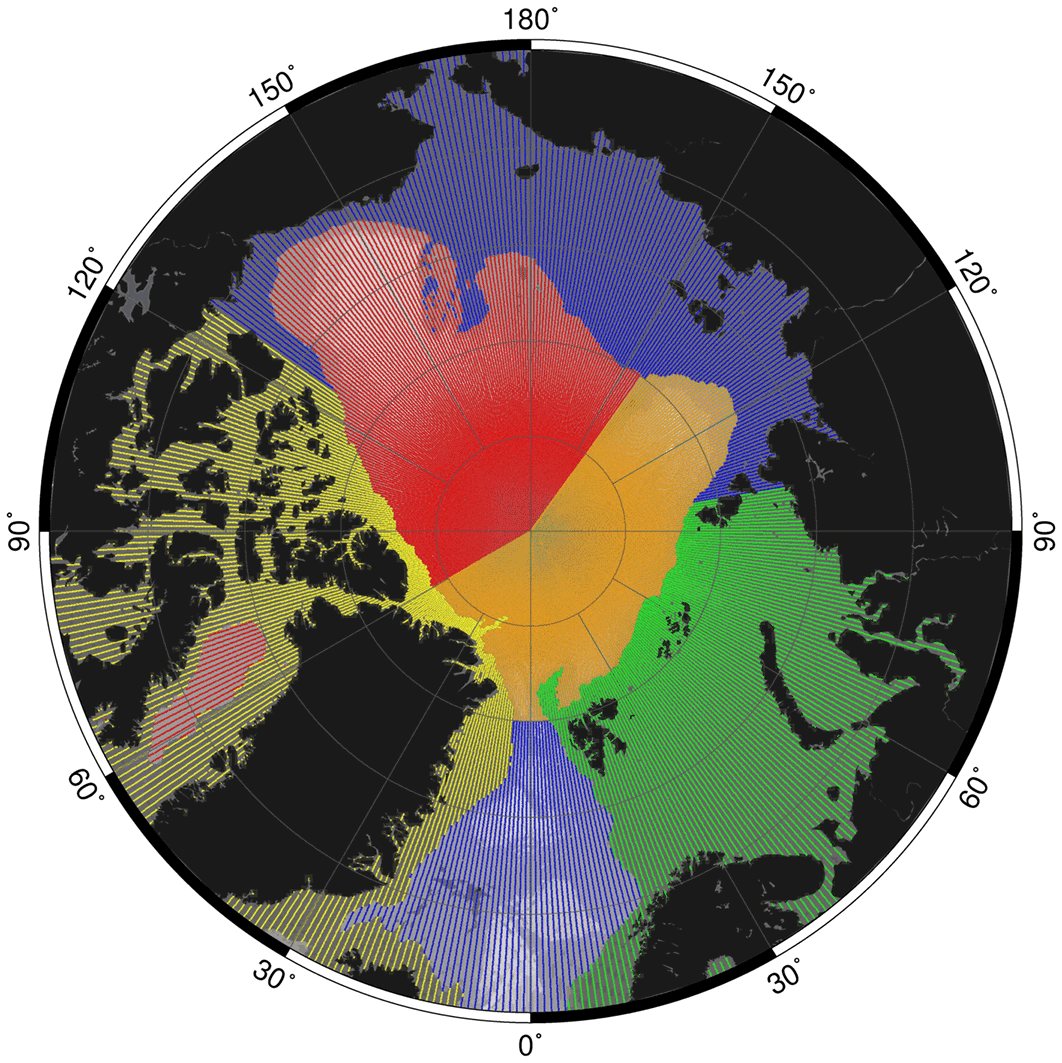
Figure 6 Regions that were used for the statistical screening (see Sect. 3). Red: Amerasian Basin. Light red: deep basin of Baffin Bay. Blue: Amerasian shelf. Light blue: Greenland–Iceland–Norwegian seas. Orange: Eurasian Basin. Green: Barents and Kara seas. Yellow: Canadian Archipelago and Greenland–Iceland shelf.

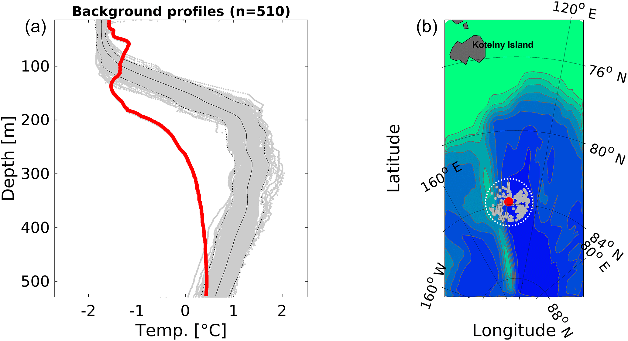
Figure 7 Sample output of the statistical screening. (a) CTD profile (red line) and 510 background profiles (grey) detected in the search window. The black solid curve is the mean temperature calculated from the background profiles, and the dashed curves are the mean ±2 standard deviations. The geographic coordinates of the tested profile are probably wrong. (b) Location of the profile (red circle) in the Amundsen Basin and the neighboring profiles (grey circles) detected in the search window.

For every profile, neighboring profiles were found in a circular window with 120 km radius (Fig. 7). In regions with high data density (i.e., Nordic, Barents and Beaufort Sea) we used a window radius of only 60 km. The window was not allowed to cross the regional boundaries to avoid comparison of data from hydrographically different environments. All profiles in the window were then interpolated to a 1 m vertical grid and then truncated to the most frequent minimum and maximum depth to ensure comparability. We then used three statistical parameters for comparison that were considered most effective by Gronell and Wijffels (2008): (a) temperature (T) and salinity (S) of a depth (z) surface, (b) the T and S gradient at z, and (c) the vertically averaged integrated T and S. A profile was flagged and visually inspected when at least one of its statistical parameters exceeded the average of the same parameter, calculated from the background field, by 4, 7 or 7 times the standard deviation, respectively (Gronell and Wijffels, 2008). The test turned out to be very sensitive. For the first two parameters we therefore flagged the profiles only when the number of suspicious values exceeded 5 % of the profile length.

In some cases, only few profiles were found in the search window, making the background statistics less reliable. In other cases some biased or erroneous profiles entered the statistics. Furthermore, the vertical interpolation sometimes introduced errors, in particular when low-resolution data (e.g., bottle data) were interpolated. These cases were considered with special care during the visual assessment. Whether a profile was biased or not was sometimes difficult to assess. A flagged temperature profile close to the background distribution may just display an exceptional event in the natural variability. In these cases we therefore excluded profiles only from bottle, XBT and MBT measurements. Moreover, an apparent bias (e.g., Fig. 7) may just display a different physical state in a certain region of the ocean (Manzella and Gambetta, 2013). We therefore always stored ID numbers of all excluded profiles to enable a reassessment of these data for future updates of the archive.

In total, 8605 temperature and 12 755 salinity profiles failed in the statistical screening. Among them are many profiles from XCTDs, as they often contain gradients that are detected as statistically significant deviations from the climatological background. A total of 2064 profiles were excluded after visual inspection in this step.

3.5 Corrections

In 1514 profiles we found multiple measurements on single depth levels. In these cases, we calculated an average for each depth level if the standard deviation of the temperature or salinity values was smaller than 0.1 units. If the standard deviation exceeded this threshold, we removed the data from the profile. Some profiles from drifting buoys and profiling floats contained negative depth gradients. These data were ordered by depth to obtain a monotonically increasing depth vector. A total of 562 profiles were truncated, mainly from XCTDs that displayed unrealistic values after the wire broke.

Table 3 Quality flags used to mark erroneous or suspicious data detected during the QC routines.

^* Full profile flagged

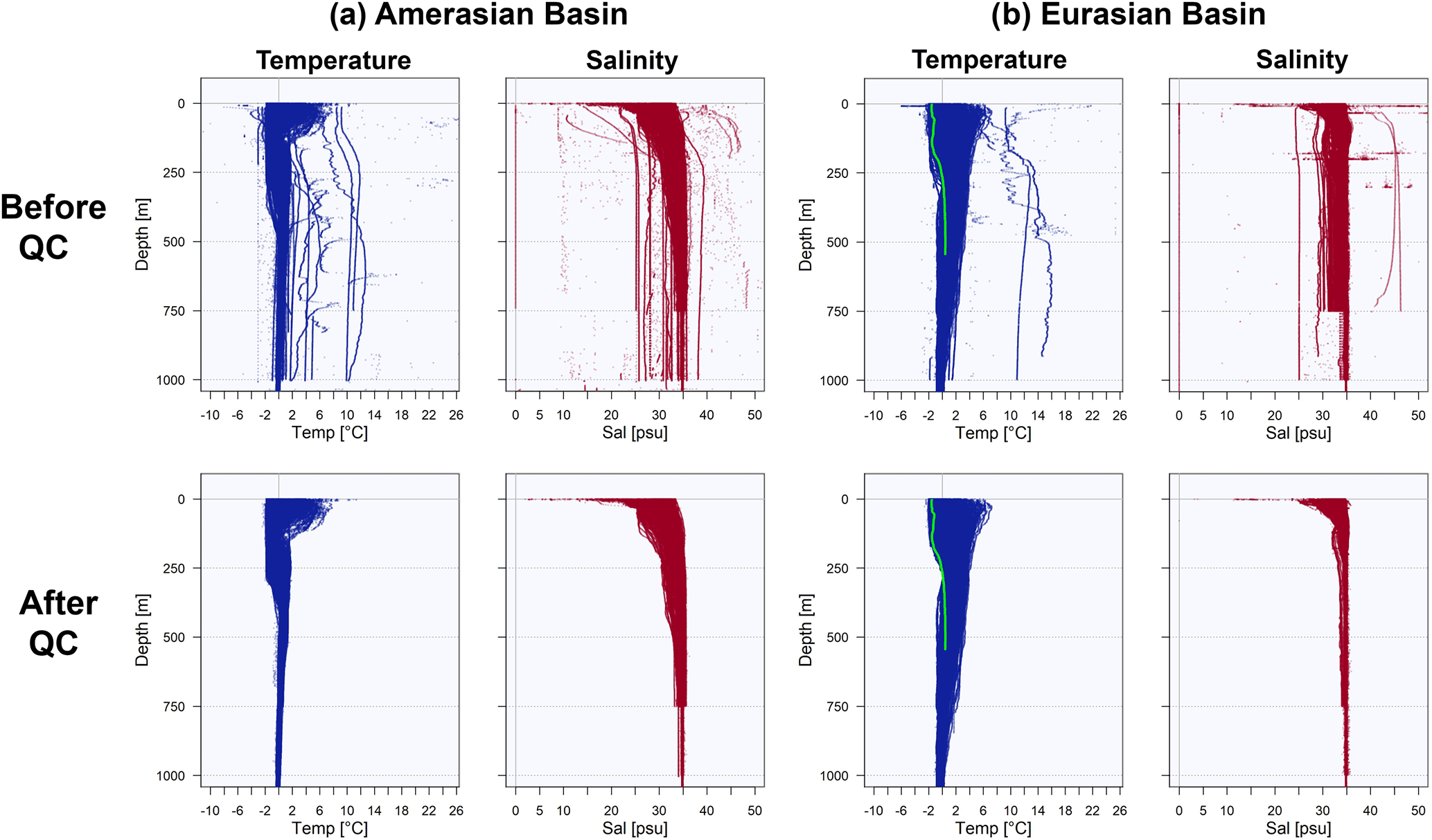
Figure 8 Temperature and Salinity from (a) approximately 37 000 profiles measured in the Amerasian Basin (see Fig. 6) and (b) approximately 17 000 profiles measured in the Eurasian Basin before (upper panels) and after (lower panels) data validation and removal of outliers. The green line in the temperature profiles of (b) is the profile from Fig. 7 that failed the statistical screening.

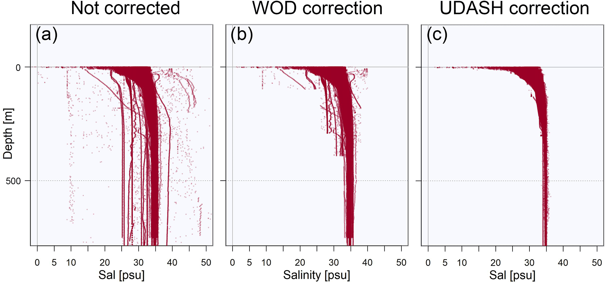
Figure 9 WOD salinity data in the Amerasian Basin. (a) Data without correction. (b) Accepted data according to the WOD quality flags. (c) Accepted data according to the UDASH quality flags.

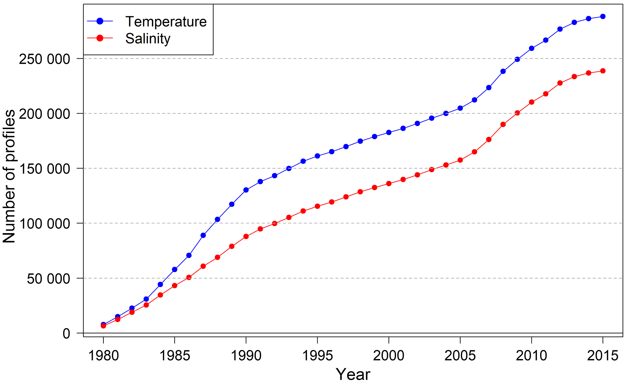
Figure 10 Evolution of the number of temperature and salinity profiles (cumulated) over the entire period.

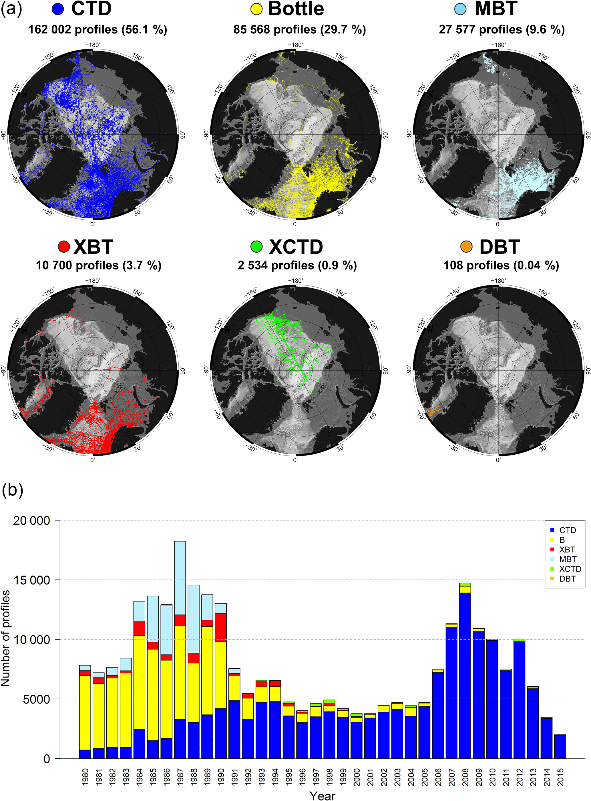
Figure 11 (a) Distribution maps of different instrument types. The fraction of the full data set is shown as percentage in brackets behind the respective number of profiles. CTD: conductivity–temperature–depth, XCTD: expendable CTD, XBT: expendable bathythermograph, MBT: mechanical bathythermograph, DBT: digital bathythermograph (only 1986). STD: salinity–temperature–depth (not shown, only few profiles exist near Point Barrow, Alaska). (b) Number of profiles per year, measured by different instrument types (1980–2015). Note the peak around the International Polar Year (IPY) in 2007–2008.

3.6 Quality flags

All profiles that were considered bad were excluded after visual assessment in one of the steps of the QC routines. However, since most of our detection algorithms are very sensitive, many other profiles and single measurements failed in one (or more) of the tests described above. These data were flagged and remain in the archive. The flags may be used for more detailed investigations of the data quality. We therefore did not discriminate between only good and bad data. Our flagging system includes individual flags for each test in our QC routines. This enables the user to, for example, easily identify all data outliers for interpolation.

Not-suspicious data are flagged with “0” (Table 3). For flagging position errors we used column 11 (quality flag for pressure and depth). Positions on which the deepest measurement was found more than 200 m deeper than the interpolated ocean bottom were flagged with “1” and suspicious positions from the cruise-track check with “2” (see step 2 for details). All depth values of a profile were flagged, as the failure affects the full profile and not only single depth levels. If a profile was affected by both errors, the column was flagged with “3”.

Temperature or salinity values that were changed and recalculated (see previous section) were flagged with “1”. Suspicious gradients were flagged with “2”, such that the gradient between the flagged value and its preceding value can be considered suspicious. This also applies to density inversions. A density inversion was flagged with “3” in both columns (13 and 15), as density was calculated from both quantities. If a profile did not pass the statistical screening, all values in columns 13 or 15 were flagged with “10”. This number was always added to the other flags. Temperature and salinity outliers were flagged in the columns 13 or 15 with “4”. For example, an outlier in a temperature profile that did not pass the statistical screening is flagged with “14”, while all other values are flagged with “10”. This means that for finding all detected outliers in the data the user has to search for flags “4” and “14” (e.g., for density inversions “3” and “13”). Many temperature and salinity values failed in more than one test in step 3 of the QC procedure. For example, an outlier can also be detected as a suspicious gradient and additionally as part of a density inversion. In these cases we always considered an outlier as the most serious error and flagged the value with “4”. If a suspicious gradient and a density inversion was detected, we considered the density inversion as more serious and flagged with “3”. Empty cells with missing or deleted data (value −999) were flagged with “5”.

4 Description of the validated data set

The example of the successful data validation for the Amerasian Basin (Fig. 8) demonstrates the effectiveness of the applied method. For example, only four biased profiles and less than 10 data outliers in the Amerasian Basin were not detected during the QC routines and had to be removed manually. Few XCTD profiles still include very noisy data that should not be deemed outliers. We leave it up to the user to decide whether to remove or filter these profiles. They can be detected by using column 5 of the data files and by finding flag +10 in column 13 and/or 15.

A quicker approach for data validation by simply cutting off all values outside a multiple of standard deviations from the mean would remove only the largest biases and outliers. The profile with the possible position error shown in Fig. 7 does not stand out from the temperature distribution in the Eurasian Basin (Fig. 8b); i.e., the error would have remained undetected. The salinity distributions in the Amerasian Basin (Fig. 9) demonstrate that the profile-by-profile check applied for UDASH significantly increased the data quality particularly in the upper 400 m, when compared to WOD.

4.1 Temporal development

In the final archive, there are significantly fewer salinity profiles than temperature profiles (Fig. 10). Up to the early 1990s a large fraction of the profiles were still recorded with XBT and MBT instruments (Fig. 11). These instruments are not capable of measuring salinity. In addition, some of the bottle data did not include salinity measurements. The number of CTD measurements was comparably low until 1990. The number of temperature profiles therefore increased more rapidly than the number of salinity profiles (Fig. 10). From 1991 onwards CTD measurements replaced the other methods more and more (Fig. 11); i.e., most of the new profiles included combined temperature and salinity measurements. The difference in the numbers of temperature and salinity profiles (approximately 50 000) therefore remains almost constant after 1991.

During the years 1980–2015 there were two periods of increased research activity in the Arctic, 1984–1990 and 2007–2012 (Fig. 11). During the first period large numbers of profiles were taken mainly by using MBTs and bottles in the Nordic Seas and the Barents Sea, as well as in Baffin Bay and the shelf seas of the Asian and Pacific sectors. The second period mainly includes modern CTD data and primarily covers the central Arctic Basins, as well as the Nordic Seas and the western Barents Sea. This period includes the International Polar Year (2007–2008) (Mauritzen et al., 2011), which was a major step forward towards long-term monitoring of the ice-covered regions of the central Arctic Ocean. The research activities are still ongoing, and it can be assumed that a high number of profiles can be maintained beyond the year 2015. The decline in the number of profiles after 2012 is a result of the limited availability of recent data, which have not yet been processed and therefore have not been entered into the public databases so far. The numbers will likely increase with future updates of the archive.

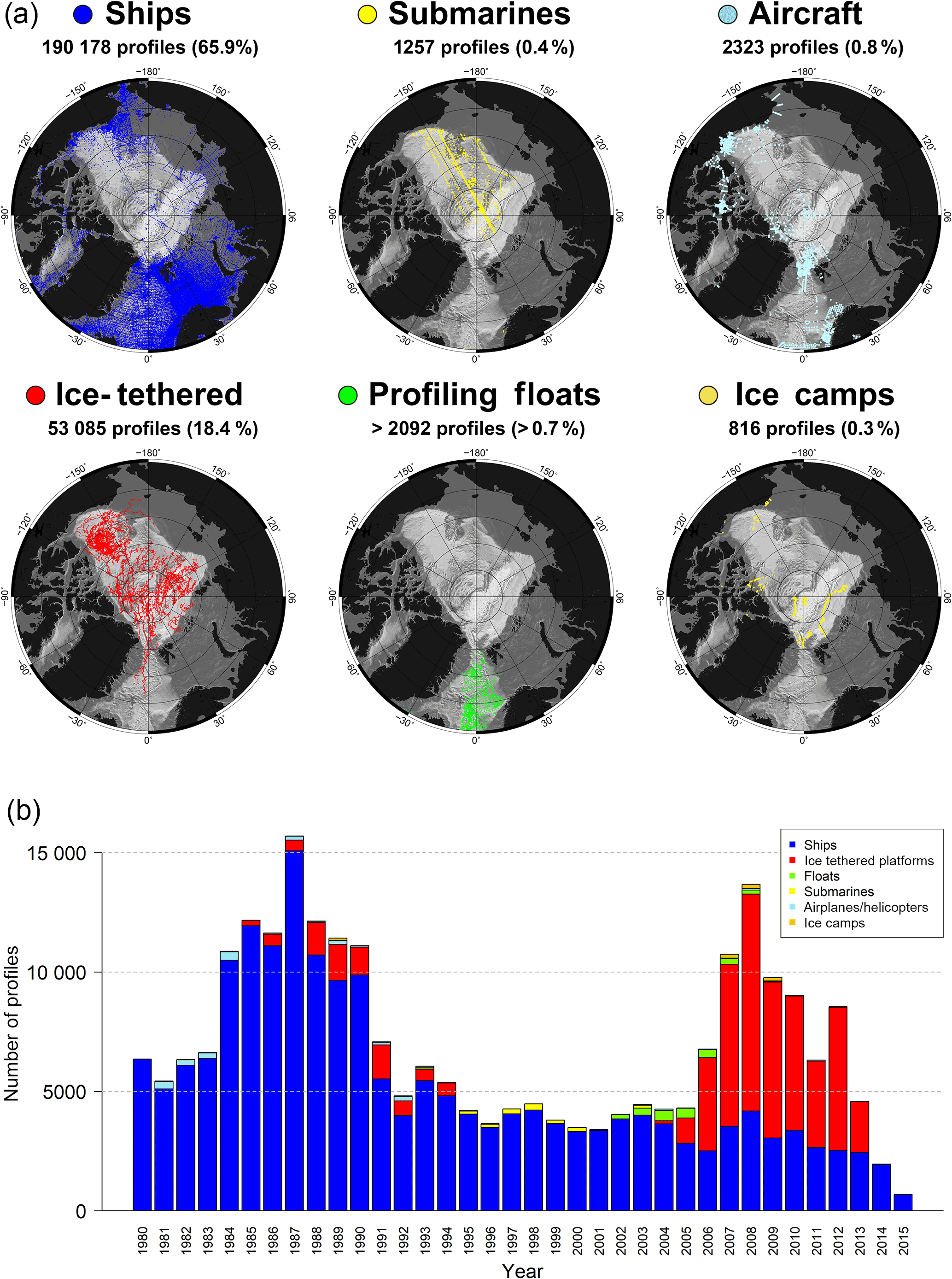
Figure 12 (a) Distribution maps of different platform types. The fraction of the full data set is shown as percentage in brackets behind the respective number of profiles. The two maps on the right-hand side are associated to some extent, as some of the airplane and helicopter surveys started from ice camps. A large number of profiles (approximately 38 000, not shown) could not be associated with a platform type in the first attempt (see text for details). (b) Number of profiles per year, measured from different platforms (1980–2015).

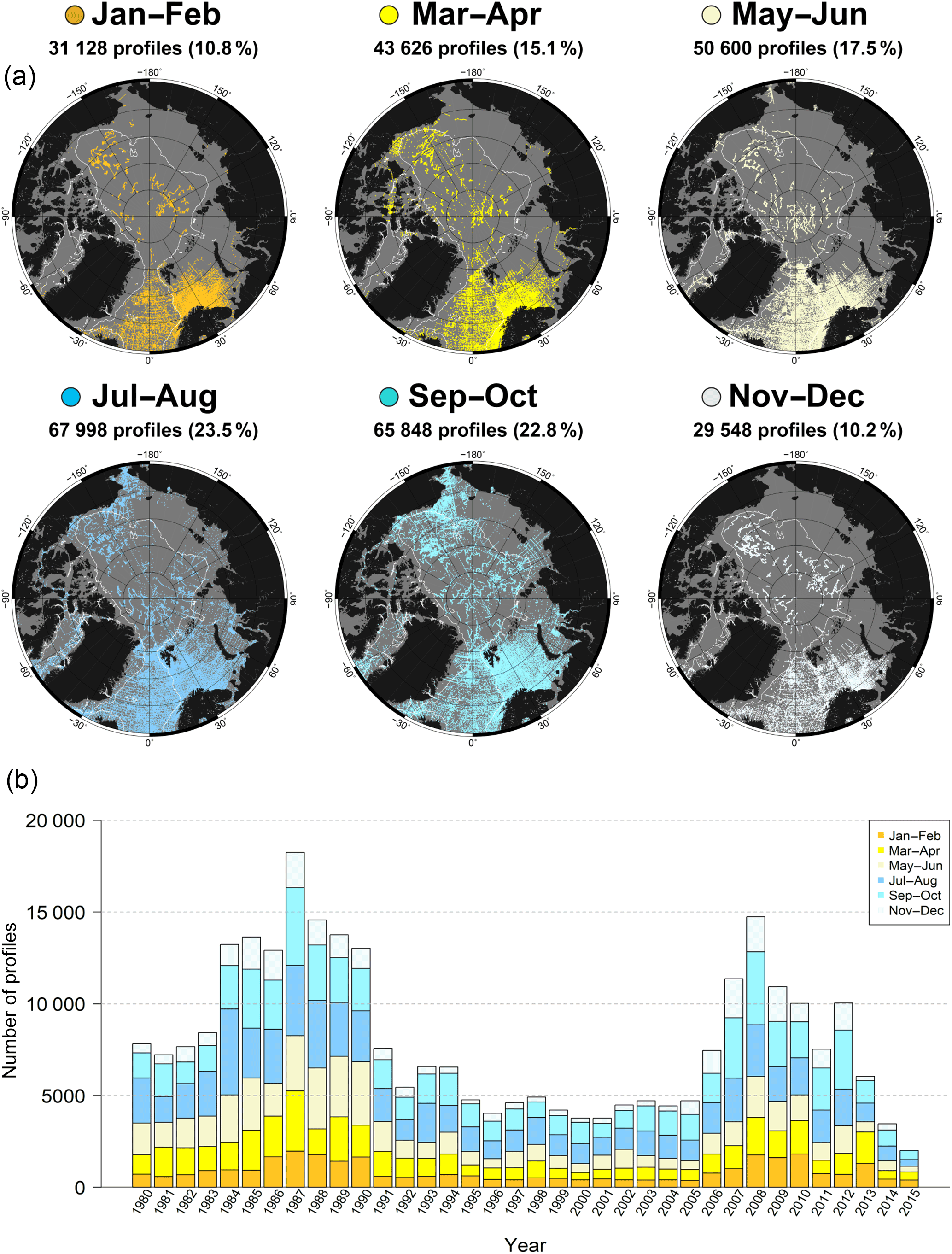
Figure 13 (a) Distribution maps of profiles in different 2-month periods. The white line is the 500 m isobath. The fraction of the full data set is shown as percentage in brackets behind the respective number of profiles per period. (b) Number of profiles per year, measured in different 2-month periods (1980–2015).

4.2 Platforms and instruments

The shift towards central Arctic measurements was possible due to the availability of modern ice-tethered profilers (Kikuchi et al., 2007; Krishfield et al., 2008). The shift goes along with a clear transition from ship-based measurements towards ITPs (Fig. 12), which displays the growing importance of these platforms. These instruments provide data from regions that are hardly accessible for ships in winter. Other ice-tethered platforms, such as under-ice moorings, were deployed from the mid-1980s to the mid-1990s. Almost 40 % (20 996 profiles) of the ITP data in our archive were measured in the months of October–January. For comparison, only 10 % (477 profiles) of the ship-based measurements in the deep basins (> 500 m) of the central Arctic were measured during these months. Almost 80 % (4818 profiles) are concentrated in the months of August and September. Other central Arctic data were measured by US submarines, mainly in the late 1990s (Fig. 12). Most of these data are part of the SCICEX program (Rothrock et al., 1999) and were collected with XCTD instruments modified for submarines (compare to Fig. 11). A small number of profiles in the central Arctic comes from drifting ice camps and aerial CTD surveys, such as the North Pole Environmental Observatory (NPEO). Profiling floats (ARGO) are still not designed for operation in ice-covered regions and provide data only for the Nordic Seas.

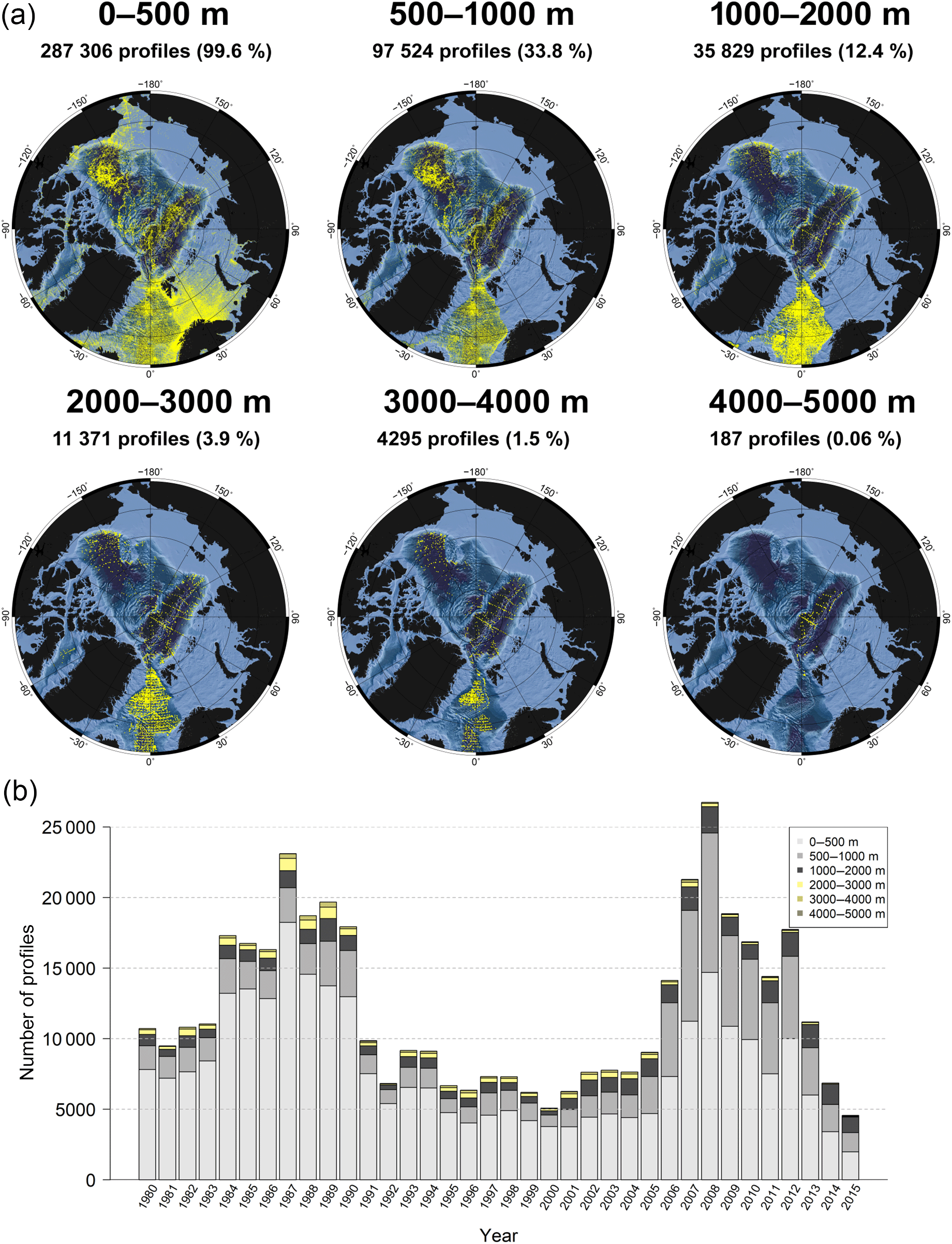
Figure 14 (a) Distribution maps of profiles with valid data in the shown depth ranges. The fraction of the full data set is shown as percentage in brackets behind the respective number of profiles. Note that the dot size varies, which makes the profile density appear higher in the Nordic Seas for the range 1000–2000 m. The percentages sum up to more than 100 % as one profile may contain data in more than one depth category. (b) Number of profiles per year, with valid data in different depth ranges (1980–2015).

4.3 Seasonal distribution

Although modern autonomous platforms measure throughout the year, there is a significant bias towards the Arctic summer (Fig. 13), as ship-based measurements still constitute a large portion of the archive (Fig. 12). The number of summer profiles is twice as high as the number of profiles measured in the winter months. But also in Spring and Autumn the amount of available data is significantly higher than in winter. From 2004 onwards the profiles increase rapidly in the months of September–November due to the deployment of ITP and POPS platforms. But also the increase in the other seasons is mainly a result of the growing ITP deployments (Fig. 12). It is obvious from the drift tracks that most of the profiles measured in the deep central Arctic basins between November and June originate from ITPs (Fig. 13).

4.4 Depth distribution

The distribution of profiles with valid data in different depth ranges (Fig. 14) shows that nearly all profiles contain data for the upper 500 m. Only a small number of profiles start below 500 m depth. For the mid-depth range 500–1000 m ITPs contribute valuable information (compare to Fig. 12). The good data coverage in the Beaufort Sea and the Eurasian Basin is mainly a result of ITP deployments. A total of 82 % of the profiles from the Eurasian and Amerasian Basins with data in the depth range 500–1000 m were measured by ITPs. Since 2006, a larger amount of data is therefore available in this range, compared to the 1980s (Fig. 14). Our knowledge about the hydrography in this region is very poor for depths deeper than 1000 m. In these two basins only 4076 (1553) profiles contribute data deeper than 1000 m (2000 m), which together constitute 1.4 % (0.5 %) of the full archive. One also has to keep in mind that these few data spread over 36 years (1980–2015). Approximately 90 % of the profiles in UDASH do not exceed the 1000 m level.

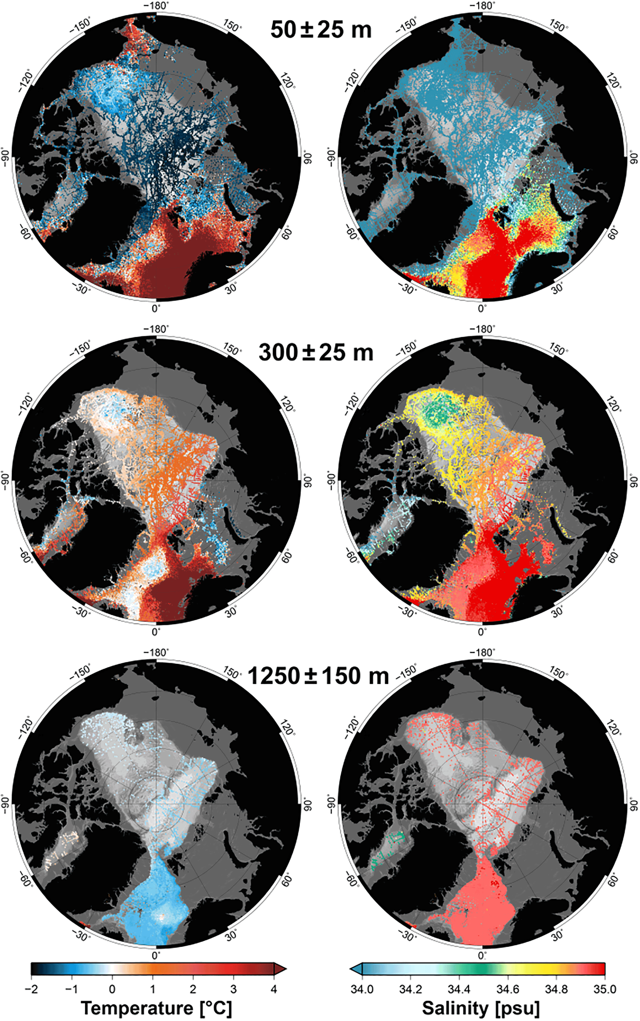
Figure 15 Temperature and salinity distribution in the Arctic Ocean for three selected depth ranges. The maps were obtained by averaging the data in the shown depth ranges for every available profile between 1980 and 2015.

4.5 Distribution of temperature and salinity

The data at the 50 and 300 m levels show the known distribution of temperature and salinity in the Arctic Ocean (Fig. 15), with warm and saline Atlantic water flowing northwards through the Norwegian Sea and entering the Arctic with the West Spitsbergen Current and, in shallow depths, through the Barents Sea (Schauer et al., 2002; Rabe et al., 2011; Seidov et al., 2015).

The 50 m level shows how cold and fresh surface waters dominate almost the entire central Arctic, with the coldest temperatures in the Eurasian Basin. The polar surface waters are transported east and west of Greenland southwards into the North Atlantic (Seidov et al., 2015). The relatively warm and fresh Pacific water, entering the Arctic through the Bering Strait, is clearly visible in the uppermost part of the map.

The 300 m level shows that the Eurasian Basin is more influenced by the inflowing Atlantic water and therefore warmer and more saline than the Amerasian Basin. Clearly visible are the colder waters in the Greenland Gyre region (e.g., Aagaard et al., 1985) and in the Beaufort Sea. In particular, in the Beaufort Sea these cold waters are associated with comparably low salinity values (Proshutinsky et al., 2002). Another clear feature is the cold deep waters in the eastern Barents Sea, which are formed in polynyas west of Novaya Zemlya through cooling and brine rejection (Schauer et al., 2002).

On the 1250 m level temperature and salinity are more or less uniform throughout the Arctic (compare to Fig. 8). An exception is Baffin Bay, with slightly warmer and fresher deep waters than in the other parts of the Arctic Ocean (Tang et al., 2004).

4.6 Ongoing and future work

Updates of the archive are planned on a yearly basis and are funded for at least the next 3 years. An update of approximately 4500 profiles from RV Polarstern was already included in the published archive. Once the data were reformatted, the QC procedures for this update were finished within 1 week. Yearly updates are therefore a realistic goal. The publication of the next updated and improved version of UDASH is planned for late 2018. We provide a WebGIS application which is a very helpful tool to easily explore the UDASH data set (http://maps.awi.de?search=udash).

4.6.1 Ongoing work

We are currently writing an extensive data documentation, which will be available on the PANGAEA web page in summer 2018. The document contains a large number of additional maps, diagrams, statistics and helpful details which facilitate the work with the database. The estimated amount of work left is 1–2 weeks.

Furthermore, we developed a quick-access tool that enables the user to extract a subset of the data by making selections, such as geographic region, instrument and time period. A preliminary version of the software already exists. It will be equipped with a graphical user interface (GUI) and provided with the first update in late 2018. The estimated amount of work for GUI programming and setup is 4 weeks.

4.6.2 Further goals for 2018

Almost 40 000 profiles (mainly from WOD) could not be associated with a certain platform type. We will attempt to identify the platforms from the metadata record and provide the information with the next update. Most of these profiles likely originate from ARGO floats and are still recognizable by a number in column 2 (cruise or platform name) of the data files. We are already in contact with experts to identify the ARGO floats by their ID numbers.

Most of the ITP profiles within UDASH still have the same cruise or platform name (e.g., itpmerged) in column 2. In one of the next steps, the single ITP profiles will be identified and renamed by using the WOD metadata. The changes will be included in the forthcoming update.

The software for exploring the WOD metadata has already been set up. The estimated amount of work is therefore 2–3 weeks.

4.6.3 Longer-term goals and perspectives

UDASH includes ITP data of different quality levels (level 2 and level 3, Krishfield et al., 2008). This information is not yet included in the metadata. We aim at including as many level-3 data as possible and will provide the information in one of the next updates.

The list of DOIs is not yet complete. Finding DOIs for individual profiles is a complex task and requires time for research. However, we will attempt to complete the list and to provide more DOIs in the next versions of UDASH.

UDASH contains approximately 15 000 profiles which are not yet part of WOD. However, most of these data will likely enter WOD in the coming years. The WOD is now the designated Centre for Marine Meteorological and Oceanographic Climate Data (CMOC) in the Marine Climate Data System (MCDS) of the Joint WMO–IOC Technical Commission for Oceanography and Marine Meteorology (JCOMM). This will ensure that all available profile data will flow into WOD and that users will find the most complete record in one place (Tim Boyer (NOAA), personal communication, 2018). UDASH would benefit from the completeness of WOD and could focus more on additional quality control and data presentation.

5 Data availability

The UDASH data are available from the PANGAEA data archive. The digital open access data library PANGAEA is a publisher for earth system science and hosted by the Alfred Wegener Institute. UDASH is stored in 36 ASCII *.txt files (one file for each year; https://doi.pangaea.de/10.1594/PANGAEA.872931) (Behrendt et al., 2017).

6 Conclusions

We compiled a high-quality oceanographic data set of temperature and salinity measurements in the Arctic, north of 65^∘ N for the period 1980–2015. The archive contains 288 532 profiles with approximately 74 million single measurements of temperature and salinity. The data were thoroughly quality tested by applying duplicate checks, position and cruise-track checks, vertical gradient checks, outlier checks, vertical stability checks and a statistical parameter screening. The tests were applied together with visual assessment of suspicious profiles to guarantee a stable data quality. Duplicate, biased and erroneous profiles were excluded from the archive, while smaller errors, such as suspicious vertical gradients, were flagged. The archive enables the user to quickly access nearly all publicly available data. It includes profiles that are not included in the World Ocean Database and provides data on a higher quality level.

The majority of the data were collected with CTD instruments and bottles from ships. During the last 10 years, however, most of the data originated from ice-tethered platforms. Only 15 % of the profiles in the archive were collected in the winter season (December–February) and 90 % of the full archive do not exceed the 1000 m level. Despite the large amount of available data, our knowledge about the deep Arctic Ocean is, therefore, still very poor, particularly for the winter months and the central Arctic Ocean. On the other hand, ITPs provide valuable information up to 750 m depth in this region.

The new data set mainly aims at oceanographic studies and provides an easy access to temperature and salinity data in the Arctic Ocean. The archive may also be used for data assimilation and validation of ocean models. We found a large amount of biased profiles, position errors, faulty cruise tracks, data outliers and unrealistic values. In total, we excluded 81 441 profiles and additionally nearly 70 000 single values because of quality problems. We therefore strongly recommend taking caution when using oceanographic data from public archives without detailed quality tests. Our data set may help the oceanographic community to quickly access large amounts of data without laborious quality testing. With our archive, we hope to facilitate Arctic Ocean research and highly appreciate any contribution with additional data that are not yet included.