the Creative Commons Attribution 4.0 License.
the Creative Commons Attribution 4.0 License.
 | 23 Jan 2018
A synthetic map of the north-west European Shelf sedimentary environment for applications in marine science
Robert J. Wilson
Douglas C. Speirs
Alessandro Sabatino
Michael R. Heath
Seabed sediment mapping is important for a wide range of marine policy, planning and scientific issues, and there has been considerable national and international investment around the world in the collation and synthesis of sediment datasets. However, in Europe at least, much of this effort has been directed towards seabed classification and mapping of discrete habitats. Scientific users often have to resort to reverse engineering these classifications to recover continuous variables, such as mud content and median grain size, that are required for many ecological and biophysical studies. Here we present a new set of 0.125∘ by 0.125∘ resolution synthetic maps of continuous properties of the north-west European sedimentary environment, extending from the Bay of Biscay to the northern limits of the North Sea and the Faroe Islands. The maps are a blend of gridded survey data, statistically modelled values based on distributions of bed shear stress due to tidal currents and waves, and bathymetric properties. Recent work has shown that statistical models can predict sediment composition in British waters and the North Sea with high accuracy, and here we extend this to the entire shelf and to the mapping of other key seabed parameters. The maps include percentage compositions of mud, sand and gravel; porosity and permeability; median grain size of the whole sediment and of the sand and the gravel fractions; carbon and nitrogen content of sediments; percentage of seabed area covered by rock; mean and maximum depth-averaged tidal velocity and wave orbital velocity at the seabed; and mean monthly natural disturbance rates. A number of applications for these maps exist, including species distribution modelling and the more accurate representation of sea-floor biogeochemistry in ecosystem models. The data products are available from https://doi.org/10.15129/1e27b806-1eae-494d-83b5-a5f4792c46fc.
- Article
(5624 KB) - Full-text XML
-
Supplement
(11317 KB) - BibTeX
- EndNote


Knowledge of the geographic variation in the sedimentary environment of the seabed is required for a wide variety of marine planning and science tasks. Benthic species have differing sediment requirements and seabed mapping can therefore help identify ecologically distinct habitats (Robinson et al., 2011). Sediment type and wave and tidal regime are important determinants of the rate of natural disturbance of the seabed (Aldridge et al., 2015; Bricheno et al., 2015). The composition of sediments also has a large influence on the consequences of anthropogenic disturbance on the seabed, particularly those due to trawling (Diesing et al., 2013). The evolution of deltas is strongly influenced by sediment composition (Edmonds and Slingerland, 2009; Falcini and Jerolmack, 2010). Mapping the sediment composition and physical environment of the seabed is therefore an integral part of understanding and managing benthic environments.
The north-west European Shelf is one of the world's sea regions most impacted by human activities (Halpern et al., 2014). These impacts are dominated by fishing, and it has been estimated that over 99 % of human impact on the seabed is from trawling (Foden et al., 2011). Existing maps of seabed sediments for this region have almost exclusively focused on the territorial waters of individual states (e.g. the British Geological Survey's DigSBS250 product) or subregions (e.g. the North Sea; Basford et al., 1993). Currently the EU Mesh project is mapping benthic habitat classes across the north-west European Shelf (Vasquez et al., 2015). However, no existing research has mapped the continuous properties of sediments across this region. Here we map key parameters related to the sediment composition and the physical environment of the seabed in an area extending from the Bay of Biscay to the northern limits of the North Sea.
This study was motivated by the need for openly available datasets of the sedimentary environment for parameterizing shelf sea ecosystem models (e.g. Baretta et al., 1995; Blackford, 1997; Heath, 2012; Ruardij and Van Raaphorst, 1995) and for habitat mapping. Hence, we set out to map mud, sand and gravel percentage compositions and a set of parameters which are of particular relevance for ecosystem modelling and habitat mapping.
A key challenge to mapping seabed sediments across the north-west European Shelf is that sediment data are unavailable across the entire region. In areas with high-quality spatial sediment data, it is relatively easy to provide credible maps of sediment composition using statistical interpolation techniques. However, an alternative method is needed where there is poor or no data coverage. Recently, Stephens and Diesing (2015) demonstrated that the mud, sand and gravel percentages of the seabed in British territorial waters and a large part of the North Sea can be predicted using random forest models (Liaw and Wiener, 2002) which have environmental conditions at the seabed as predictors. Further, other work has shown clear relationships between the sediment composition of the sea floor and the energetic regime at the sea floor (Porter-Smith et al., 2004; Ward et al., 2015; Heath et al., 2016).
We extend this method by predicting the sediment composition of the seabed across the entire north-west European Shelf. However, our approach to mapping differs from that taken by Stephens and Diesing (2015), who only mapped predictions of sediment composition. Since these predictions will be less reliable than interpolated values in regions with good data coverage, we interpolate sediment composition where data are available and predict it where it is not, thus creating a synthetic picture of the seabed over the north-west European Shelf. Further, we expand the approach of Stephens and Diesing (2015) and map a number of other key parameters including seabed rock, median grain sizes of the whole sediment, sand and gravel fractions, and porosity and permeability; the outputs of these models are combined with time series of tidal and wave orbital velocities and a model of natural disturbance to provide a map of natural disturbance rate on the shelf.
The motivation for the choice of seabed parameters is as follows. Mud, sand and gravel percentages and rock cover are key determinants of the suitability of a habitat for benthic species (Gray, 2002; Thrush et al., 2003), and they strongly influence the median grain size of sediments, which plays a key role in determining the natural disturbance of the seabed (Aldridge et al., 2015). Similarly, the median grain size of the sand and gravel fraction play key roles in the properties of sandy and gravelly sediments. The median grain size of the mud fraction is critical for cohesion in muddy regions, but there are insufficient data for this to be mapped credibly. A complete representation of seabed biochemistry in ecosystem models requires knowledge of porosity and permeability, which are related to whole-sediment median grain size (Ruardij and Van Raaphorst, 1995; Lohse et al., 1993). The carbon and nitrogen content of seabed sediments were mapped because of their importance to benthic communities, sediment resuspension and the potential importance of sediment carbon stores in national carbon inventories (Avelar et al., 2017). Quantitative information about the physical environment on the seabed is necessary for the production of benthic habitat maps (Vasquez et al., 2015) and as a means to compare rates of natural and physical disturbance (Diesing et al., 2013).
Table 1Data products created at a spatial resolution of 0.125∘ by 0.125∘.
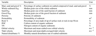
Table 2Summary of data sources used in sediment analysis. Datasets 1 (http://www.bgs.ac.uk/geoindex/wms.htm) and 8 (http://www.vliz.be/vmdcdata/nsbs/) were open access. Datasets 3, 4, 5, 9, 10 and 12 were available from the transnational database of North Sea sediment data (Valerius et al., 2015), which is a collation of data compiled by the EMODnet-Geology (http://www.emodnet.eu/geology), TOLES (http://www.belspo.be/belspo/brain-be/projects/TILES_en.PDF) and AufMod (http://www.kfki.de/de/projekte/aufmod) projects. Datasets 2, 6 and 7 were available from institutional contacts. Dataset 11 was downloaded from https://jetstream.gsi.ie/iwdds/index.html.
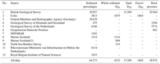

Figure 1Region where the sedimentary environment was mapped. We defined the north-west European Shelf as the region between 17∘ W and 9∘ E and 44 and 63∘ N, where bathymetry was less than 500 m. The solid black line demarcates the region where tidal velocities were taken from the Scottish Shelf Model, as described in Sect. 2.2.4.
2.1 Overview
Our goal was to produce synthesized maps of the sedimentary environment of the north-west European Shelf, which we define to be areas shallower than 500 m within the longitude and latitude range 17∘ W to 9∘ E and 44 to 63∘ N (Fig. 1). There are minimal sediment data for deeper areas within this region and almost all of the observations are dominated by mud (George and Hill, 2008), so it is reasonable to assume that these regions are comprised largely of mud and will have negligible natural disturbance rates. Data products were created with a spatial resolution of 0.125∘ longitude by 0.125∘ latitude and are listed in Table 1.
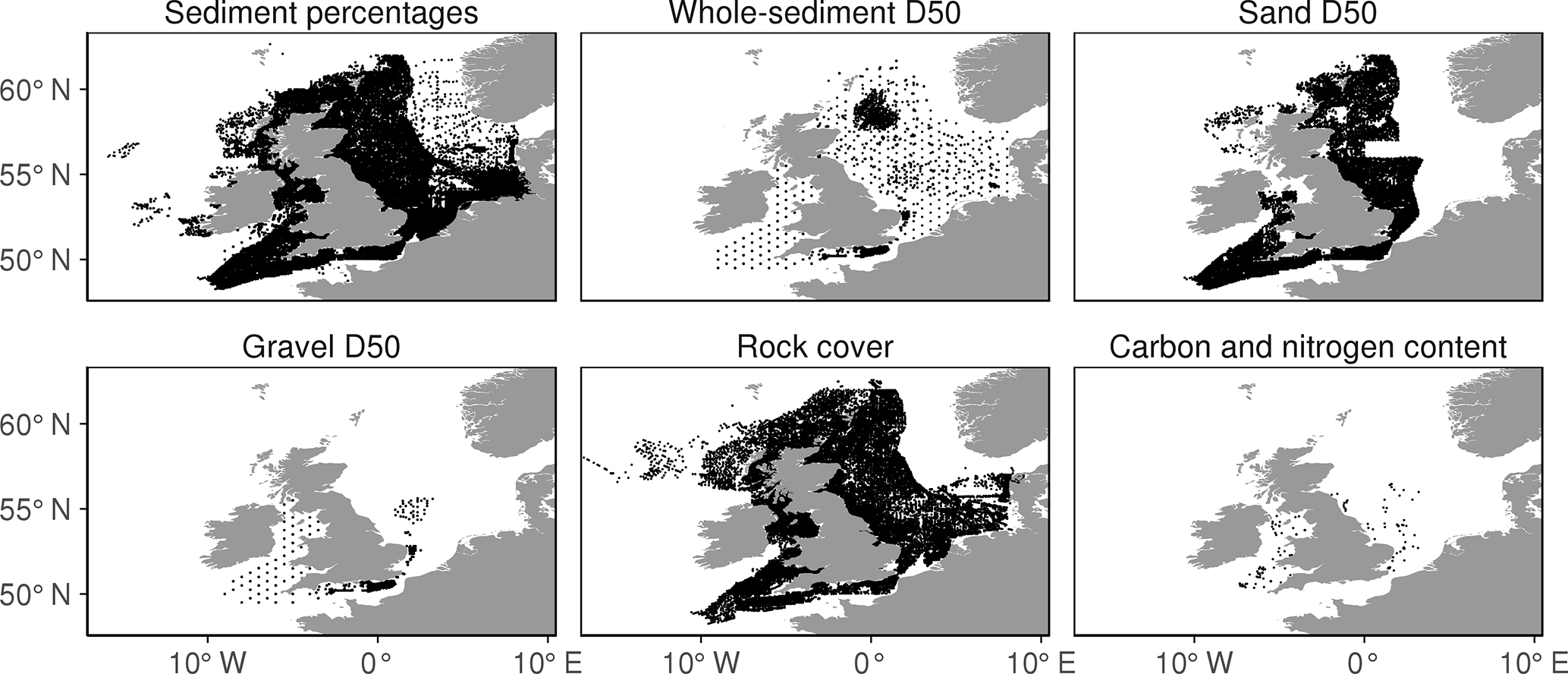
Figure 2Locations with field estimates of each seabed sediment parameter. Data sources are listed in Table 2.
Seabed sample coverage of this shelf region is highly heterogeneous with large expanses of the domain lacking accessible data. Hence, our strategy was to fill these voids in the sample coverage with statistically modelled values. The steps involved in mapping the sedimentary environment were therefore as follows.
-
Sediment data from a number of sources (Table 2) were compiled to create a composite dataset of mud, sand and gravel percentages, rock cover, carbon and nitrogen content of sediments, and median grain sizes.
-
In areas where we have data, we spatially interpolate the relevant statistic onto the study grid.
-
Using observations, we developed random forest (RF) models to predict sediment composition using wave and tidal velocities, bathymetric properties of the seabed and distance from the coast.
-
We then used RF-predicted values to infill regions of the mapping domain where the observed data density was insufficient for direct gridding.
-
Sediment porosity and permeability at each map grid point were derived from the whole-sediment median grain size using empirically based relationships assembled from literature data.
-
The natural disturbance rates of sediments at each gridded location were then calculated from wave and current bed shear stress and grain size estimates using sediment dislocation theory.
2.2 Data sources
2.2.1 Raw sediment data and processing
We compiled data on the sediment composition of the seabed from a large number of sources. Our analysis uses the following data: mud, sand and gravel percentages, rock cover and the median grain size of the whole sediment, sand fraction and gravel fraction. The data sources are summarized in Table 2 and the geographic locations where sediment data were available are shown in Fig. 2.
The British Geological Survey (BGS, 2013) provides mud, sand and gravel percentages and the median grain size of the sand fraction for locations in most of the United Kingdom's territorial waters. Data were downloaded from the BGS website using the offshore GeoIndex tool (http://www.bgs.ac.uk/geoindex/wms.htm). The raw BGS dataset included 26 259 records of sediment composition. However, to provide a consistent measure of mud, sand and gravel content we only used grab samples. This reduced the total number of records of sediment percentages and sand D50 records to 20 857 and 13 289 respectively.
An extensive dataset of surface mud, sand and gravel percentages was compiled for the transnational database of North Sea sediments (Valerius et al., 2015). This provides 36 997 records of sediment composition, with data coming from historical records of the Federal Maritime and Hydrographic Agency (Germany), the Geological Survey of Denmark and Greenland, the Geological Survey of the Netherlands, Rikswaterstatt (the Netherlands), and the Royal Belgian Institute of Natural Sciences.
Records of whole-sediment median grain size were available from the North Sea Benthos Survey (NSBS) (Basford and Eleftheriou, 1988; Basford et al., 1993). NSBS data were downloaded from the http://www.vliz.be/vmdcdata/nsbs/ website. In total there were 219 records of the whole-sediment median grain size. These data are available as separate webpages for each location and we used the rvest package in R to convert the html code into columned csv format.
The Centre for Environment, Fisheries and Aquaculture Science (Cefas) provided sediment data which included the mud, sand and gravel percentages and the distribution of sediments by grain size. Data provided by Cefas covered a large part of English and Welsh waters. In total, Cefas provided 3814 records of mud, sand and gravel percentages and sediment distribution. However, to provide a consistent estimate of sediment type we restricted our analysis to sediments analysed using laser methodology and from the top 10 cm of the seabed. This resulted in a total of 1879 sediment records being used. Cefas did not provide estimates of median grain size. We therefore calculated the median grain size as follows. For the sediment record at each location, a cumulative curve of sediment weight percentage was calculated. We then calculated the median point of this curve and classified this as the median grain size. This was carried out for the entire sediment and also for the gravel fraction.
Two datasets were provided by Marine Scotland. The first included mud, sand and gravel percentages and whole-sediment median grain sizes for a large part of the North Sea. In total, this dataset had 1214 sediment records. The second dataset included estimates of the median grain size of the combined mud and sand fraction. These grain size data were not directly usable, so we filed out samples in which the percentage of gravel was small enough that the median grain size of the mud–sand fraction was close to that of the whole sediment. To do this we analysed Cefas data and established that when the whole-sediment D50 is calculated with and without the gravel fraction for sediments with less than 10 % gravel, there is negligible difference between the estimates of D50. We therefore used the BGS dataset to identify regions where the gravel fraction was below 10 %. This was carried out by first calculating the number of BGS observations in each 0.5∘ N by 1∘ W cell. We excluded cells with fewer than 10 observations. We then further excluded all cells in which more than 10 % the observations had 10 % of higher gravel content. In these regions we accepted the Marine Scotland data as a reasonable estimate of the whole-sediment D50.
The Infomar project (http://www.infomar.ie) is mapping the seabed in Ireland's territorial waters. It has compiled a historical dataset of grab samples which show the surface mud, sand and gravel percentages in many locations in Irish waters. Data were downloaded in shape file format from the https://jetstream.gsi.ie/iwdds/map.jsp website. In total, there were 1392 records of surface sediment composition.
2.2.2 Rock data
Our aim was to classify locations as non-rock, rock at surface (i.e. approximately the top 10 cm of sediment) and rock in the approximately top 50 cm of sediment and to map the percentage of surface area in each rock classification. Historically, areas have only been mapped in a discrete fashion (e.g. the British Geological Survey's Digirock map; Gafeira et al., 2010), with relatively broad areas placed in one rock category or another. Further, there are no published large-scale datasets explicitly identifying whether locations have rock at or near the sea floor. We therefore created a composite dataset using historical survey logs for British territorial waters and borehole records for the territorial waters of Denmark, Germany and the Netherlands.
The British Geological Survey provides a database of downloadable historical logs of sediment sampling surveys (available from http://www.bgs.ac.uk/geoindex/wms.htm) with good spatial coverage for British territorial waters. These logs come in the form of scanned PDFs, and they provide written summaries of each sampling event. The analysis was restricted to corer records, which typically provided sufficient information to determine if there was strong evidence of rock at or near the seabed. Grab sample survey data were initially analysed; however, the use of grab sample records will underestimate rock levels as the grab can return sediment despite there being rock at or close to the surface. We therefore ignored grab samples.
Before analysing the PDFs we created the following categories for the records: (1) evidence shows there is no rock at the location; (2) written logs are consistent with rock at the surface or rock covered by a thin skin of sediment (approximately 10 cm); (3) written logs show that there is probably a significant layer of sediment covering rock; (4) ambiguous or an unreadable record. A Python script was written that will move through each PDF and allow an analyst to classify it. This process was randomized to ensure there was no spatial bias in classification error. In total there were 20 709 initial PDFs. Of these 149 could not be classified as rock or non-rock and were discarded. There were 18 871 records with no evidence of rock, 747 with evidence of rock at or near the surface and 942 records showing rock in the top 50 cm.
Borehole records provide reliable records of the rock composition of the seabed and the layers below it. German borehole data are available from the Geopotenzial Deutsche Nordsee project. The http://www.gpdn.de/ website provides visual records of borehole logs at a large number of locations in German territorial waters in the North Sea. A total of 862 records were visually inspected and we found no evidence of rock at or near the surface in any record. The Geological Survey of the Netherlands provides extensive borehole data. These were downloaded as individual text files from the https://www.dinoloket.nl/en/subsurface-data website. Each text file provided a record of the sediment type in each layer of the borehole in a consistent format. We first identified whether there was rock in the top 50 cm of any of the core records and found none. We therefore found no evidence of surface rock in Dutch waters. The Geological Survey of Denmark and Greenland provides borehole data for Danish waters in the North Sea. Data were available from the http://www.geus.dk website. Each borehole record is available as a separate webpage, and we therefore used the R package rvest to save the relevant html code and convert the depth profile of sediment type to csv format. We were then able to identify the sediment type in the top 10 and 50 cm at each location.
2.2.3 Carbon and nitrogen content
Diesing et al. (2017) showed that the carbon content of sediment could be credibly predicted based on a series of environmental predictors. Here we take a similar approach to the predictive mapping of the carbon and nitrogen content of sediments. Particulate organic carbon (POC) and total nitrogen (TN) content were downloaded from the Cefas Data Hub (https://doi.org/10.14466/CefasDataHub.32) and taken from Serpetti et al. (2012). It is clear that carbon and nitrogen levels in sediment are strongly determined by mud content (Serpetti et al., 2012), and each record of carbon and nitrogen content is associated with a field estimate of mud content. We therefore used mud as a predictor. However, the mud measurements in the Cefas dataset alternate between using laser and sieve methodology and therefore do not provide consistent and comparable estimates of mud content. The Cefas dataset contained 182 sediment samples for which the mud content was estimated using laser and sieve methodology, which showed a strong statistical relationship between each measure. We therefore converted each sieve estimate of mud content to a laser equivalent using a statistical relationship modelled using the lm function in R (laser mud = 3.157 × (sieve mud)0.7225, p value: , r2=0.93) (Fig. 3).
2.2.4 The physical environment
Depth-averaged tidal velocities were calculated as follows. For most of the study region tidal velocities were taken from the output of the Scottish Shelf Model, which is an implementation of the unstructured, finite-volume 3-D hydrodynamic model FVCOM. The spatial domain of this model covers approximately 80 % of our study domain (Fig. 1). A full description of the model is provided by De Dominicis et al. (2017), and here we use the same model run described therein. A 1-year climatology (for the years 1990–2014) of atmospheric forcings was used to run the model.
For the rest of the model domain we derived tidal velocities as follows. The Oregon State University Tidal Prediction Software (OTPS) is a well-known open-source barotropic tidal model based on the Oregon State University tidal inversion of TOPEX/POSEIDON altimeter data and tide gauge data (Egbert et al., 2010). This model was used to derive the relevant tidal components. The model can be obtained from http://volkov.oce.orst.edu/tides/otps.html. We obtained a regional tidal solution using the Oregon State University Tidal Inversion Software (OTIS) with a spatial resolution of 1/30∘. The model satisfies the depth-integrated two-dimensional shallow water equations describing momentum balance as follows:
and volume conservation
where η is sea surface elevation, u is the horizontal velocity vector, f is the Coriolis parameter, F is the fractional damping, AH is an eddy coefficient, which is assumed to be constant, H is bathymetry and ηEQ is the equilibrium tide allowing for the body tide, tidal self-attraction and loading.
Wave conditions were acquired from the ERA-Interim reanalysis (Dee et al., 2011). Significant wave height, mean wave period and mean wave direction were downloaded from the ECMWF website at http://www.ecmwf.int/en/research/climate-reanalysis/. The ERA-Interim reanalysis has a spatial resolution of approximately 79 km and a temporal resolution of 6 h. Orbital velocities at the seabed were calculated using the equations of Soulsby (2006), and the relevant equations are given in this paper's Appendix. Bathymetry for the wave and tidal model runs was attained from the high-resolution (30 arcsec) General Bathymetric Chart of the Oceans (GEBCO). With the exception of the Scottish Shelf Model output we used 2012 as the year for analysis of wave and tidal conditions.
To calculate the bed shear stress we used the equations of Soulsby and Clarke (2005) under combined wave and currents conditions on smooth and rough beds. This set of equations is reproduced in the Appendix to this paper. Root mean square shear stresses for waves plus currents were used. The calculation of bed shear stress requires the bathymetry, depth-averaged current speed, current direction, significant wave height, wave period and wave direction.
For the statistical modelling of sediment composition we used EMODnet bathymetry data. These have a spatial resolution of 1/8 arcmin by 1/8 arcmin and were downloaded from the EMODnet website (http://www.emodnet.eu/bathymetry/). Data processing and calculations were carried out in R using the packages dplyr (Wickham et al., 2017) and Rcpp (Eddelbuettel et al., 2011).
2.3 Spatial gridding and predictive modelling
The synthetic maps of mud, sand and gravel percentages, and rock cover were created as follows. First we identified regions where a statistical interpolation of the relevant parameter would give a reasonable estimate across that region. In other regions we used statistical models to predict the parameter. We assume that the environmental drivers of sediment composition are consistent across space.
Sampling coverage of sediment composition covered almost all of the North Sea, the United Kingdom's territorial waters and parts of Ireland's territorial waters (Fig. 2). Observations almost universally come from sampling programmes that aimed to provide consistent spatial coverage of a specific region (e.g. the North Sea Benthos Survey; Basford et al., 1993), and parameters can be interpolated in those regions. These regions were selected by creating an alphahull around each unique set of coordinates using the R package alphahull (Pateiro-l and Rodr, 2010). An alphahull is a convex envelope around the data points which will exclude areas outside the sampled regions and exclude large holes in the data coverage. Data were first interpolated onto a 1/16∘ by 1/16∘ grid and then means were calculated for each 0.125∘ by 0.125∘ cell. Parameters were spatially interpolated using bilinear spline interpolation using the interpp function from the R package akima (Akima and Gebhardt, 2016).
For areas outside the alphahulls we used random forest (Liaw and Wiener, 2002) models to predict each parameter. This class of model has been used to predict seabed sediments (Diesing et al., 2014; Huang et al., 2012; Li et al., 2011) and carbon and nitrogen content (Diesing et al., 2017). Random forest was developed by Breiman (Breiman, 2001). It is an ensemble-based modelling approach that makes no assumptions about the form of the relationships between predictor and response variables, does not require extensive parameterization, performs internal cross-validation and avoids over-fitting. Random forest takes an ensemble-based approach to regression. This is carried out by first growing a number of regression trees (Loh, 2011). Each tree is composed of a bootstrapped sample from, and of the same size as, the fitting data. Bootstrapped samples are drawn with replacement. Each split in the tree-building process only uses a subset of the predictor variables. Splitting the trees in this way reduces the dominance of individual variables and thus decorrelates the trees, making the trees less variable and more reliable (James et al., 2013). The average across all trees is then used for predictions. This ensemble averaging makes random forest robust to over-fitting (Breiman, 2001).
The observed mud, sand and gravel percentages summed to 100. However, there is no guarantee that separately predicted mud, sand and gravel percentages will sum to 100. We therefore predicted the mud, sand and gravel percentages separately and then a multiplier was applied to each prediction so that the predictions were adjusted to total 100. Random forests were created in R using the ranger package (Wright and Ziegler, 2017), which is a computationally efficient implementation of random forest for high-dimensional data. The number of trees was set to 2000, with mtry set to 3.
A similar process was carried out for median grain sizes and carbon and nitrogen content. Grain size data were available for large parts of the United Kingdom's territorial waters and some parts of the North Sea, while carbon and nitrogen content were exclusively available in parts of the United Kingdom's territorial waters (Fig. 2). First we used the alphahull approach to identify regions where we can interpolate the parameter. We then used statistical models (discussed in Sect. 2.3.1) to predict each parameter. In each case the sediment percentage maps discussed above were used as predictors in the mapping exercise. Maps and figures were produced using the R package ggplot2 (Wickham, 2016) and ternary diagrams were produced using the R package ggtern (Hamilton, 2017).
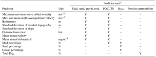
Table 3Predictors used for statistical models for predicting sediment parameters. When mud, sand and gravel percentages and whole-sediment median grain sizes were used as predictors, raw field data were used in the creation of the statistical models, whereas the synthetic maps created in this study were used for model predictions.
2.3.1 Environmental predictors for random forest models and model validation
The environmental predictors used for the random forest models that predicted mud, sand and gravel percentage, rock cover, and carbon and nitrogen content are listed in Table 3. Predictors were chosen based on a review of evidence on the environmental influences on the seabed and the requirement that data were available at the necessary spatial resolution.
Tidal and wave energy levels at the seabed should strongly influence mud, sand and gravel percentages. Large grain sizes require more energy to dislodge from the seabed, and therefore high bed shear stress is associated with increases in average grain size and reductions in mud content (Ward et al., 2015; Heath et al., 2016). There is scarce evidence to determined if seabed composition is influenced by year-round bed shear stress or individual high-energy events. We therefore used mean and maximum annual tidal and wave orbital velocities as predictors in the models of sediment composition and carbon and nitrogen content. The supply of sediment from river discharges and coastal erosion influences seabed sediment composition and carbon and nitrogen. We therefore included distance from the coast as a model predictor. The distance from the coast was calculated as follows. Shape files of coasts were attained from the Global Self-consistent, Hierarchical, High-resolution Geography (GSHHG) Database (Wessel and Smith, 1996). Distance of each data point from the coast was then calculated using the R package geosphere (Hijmans et al., 2012).
Smoothness of the seabed will influence seabed disturbance and sediment accumulation and is likely an indicator of the existence of rocky outcrops. We therefore included measures of seabed roughness as predictors in each random forest. A number of methods exist to quantify the roughness of the seabed (Wilson et al., 2007). However, many of them are not independent of the slope of the sea floor and are arguably not purely measures of roughness. For example, the standard deviation of bathymetry would classify a steeply sloping but smooth part of a continental shelf as being very rough. We therefore used the standard deviation of slope and the standard deviation of the residual topography as predictors in the random forests. Residual topography is the difference between the bathymetry at a specific point and the mean bathymetry within a specified spatial window. The residual topography was calculated using a 25-cell moving window. First the mean bathymetry was calculated within each window. The standard deviation of residual topography (σ) was then calculated using the formula of Cavalli et al. (2008): , where xi is the bathymetry in a specific cell in the moving window and the respective moving window mean bathymetry. Slope was calculated using the slope function from the R package SDMTools (VanDerWal et al., 2014). We then calculated the standard deviation of slope in a similar 25-cell moving window.
The above predictors were used for the mud, sand and gravel percentage and rock cover models. For the models of carbon and nitrogen content we also included chlorophyll, salinity and seabed temperature. Carbon and nitrogen content are influenced by biological activity and should thus be influenced by primary production levels and temperature at the seabed. The MetO-NWS-REAN-PHYS-bed-daily reanalysis was used for seabed temperature. These data were downloaded from the Copernicus Marine Environmental Monitoring Service website (http://marine.copernicus.eu/services-portfolio/access-to-products/). Daily seabed temperatures from 1995–2014 were interpolated onto each location and an annual climatology was calculated for each model grid point. Climatological (1997–2015) annual mean chlorophyll (mg m−3) data were derived from the level 4 North Atlantic chlorophyll concentration from satellite observations reprocessed data product, which is available from the Copernicus website. Proximity to river outflows likely influences levels of carbon and nitrogen, and salinity levels act as a proxy for this. We therefore calculated an annual climatological mean (1985–2014) of salinity from the MetO-NWS-REAN-PHYS-monthly-SAL reanalysis product available from the Copernicus website.
Our methodology involves predicting the sedimentary environment in geographically distinct regions. We therefore tested the ability of random forest models to do this credibly by using a cross-validation technique involving spatially disaggregated training and test datasets. Spatial disaggregation has been shown to be a reasonable method to avoid the excessive overconfidence that can possibly result from other training and testing methodologies of spatial models (Bahn and McGill, 2013; Roberts et al., 2017). The cross-validation method was as follows. We chose to use the spatial blocking method from Roberts et al. (2017). This places data into consistently sized and spatially separate blocks or bins. We chose to bin data at a resolution of 1∘ longitude by 1∘ latitude. We then used 100 iterations in which each bin was randomly assigned to training and test datasets. In each iteration the random forest was trained using the training dataset and this model was then used to predict the relevant parameter using the test data. We therefore evaluated the predictive ability of the model by calculating the mean value of each statistic in the test data for each 0.125∘ by 0.125∘ cell. The number of observations, and thus the observation reliability, in each cell varies significantly. We therefore calculate the weighted r2 between predicted and observed values in each cell, with the number of observations used as the weighting value. Weighted correlation coefficients were calculated using the function corr from the R package boot (Canty, 2002). For the full predictive models over the entire European shelf we retrained the random forests using all available data.
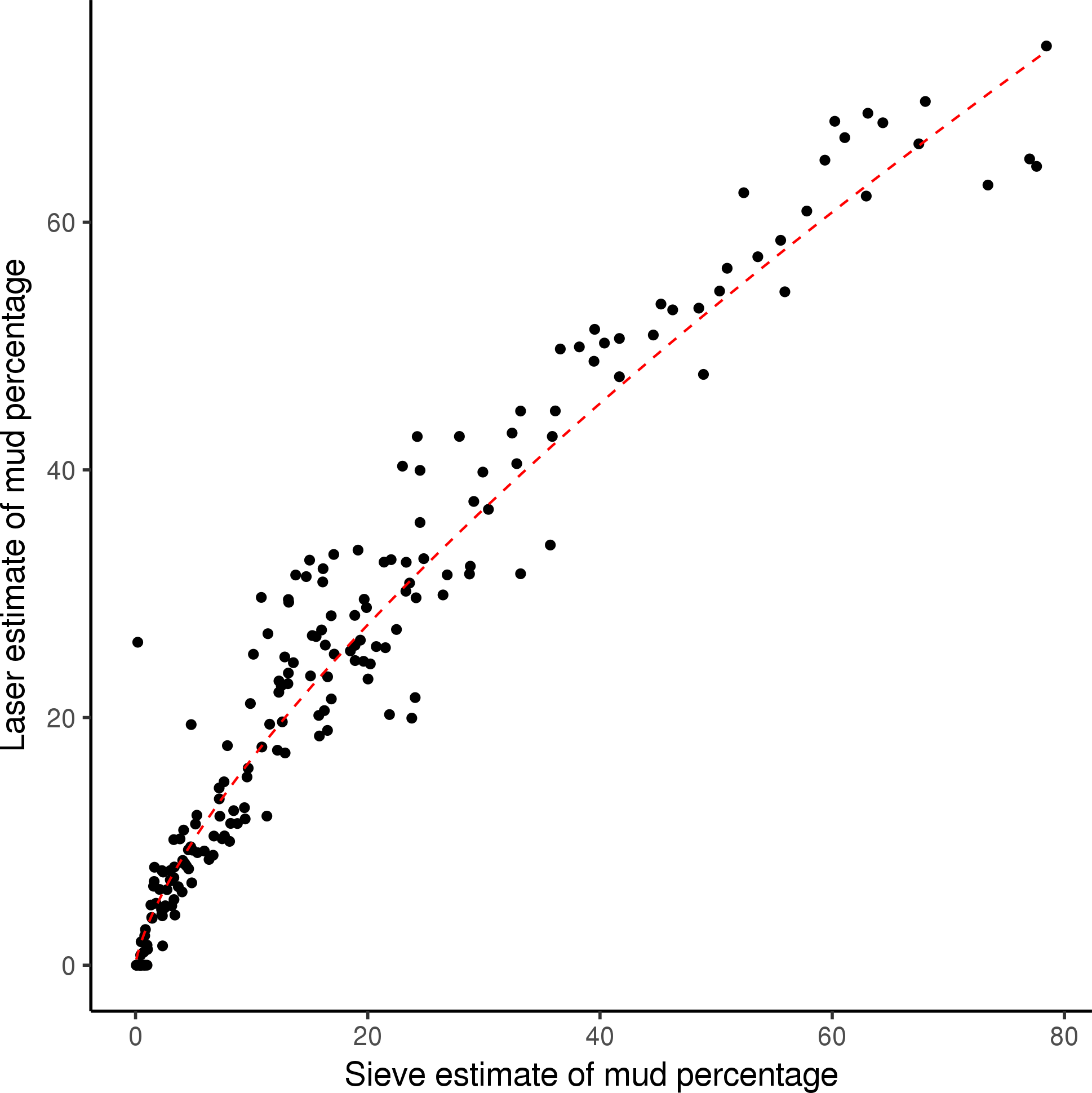
Figure 3The relationship between mud estimated from laser and sieve methodology for the same samples. For estimates of carbon and nitrogen content with only sieve-based estimates of mud content, we estimated what the mud percentage would be when calculated using laser methodology. The dashed red line shows this relationship (laser mud = 3.157 × (sieve mud)0.7225, p value: , r2=0.93).
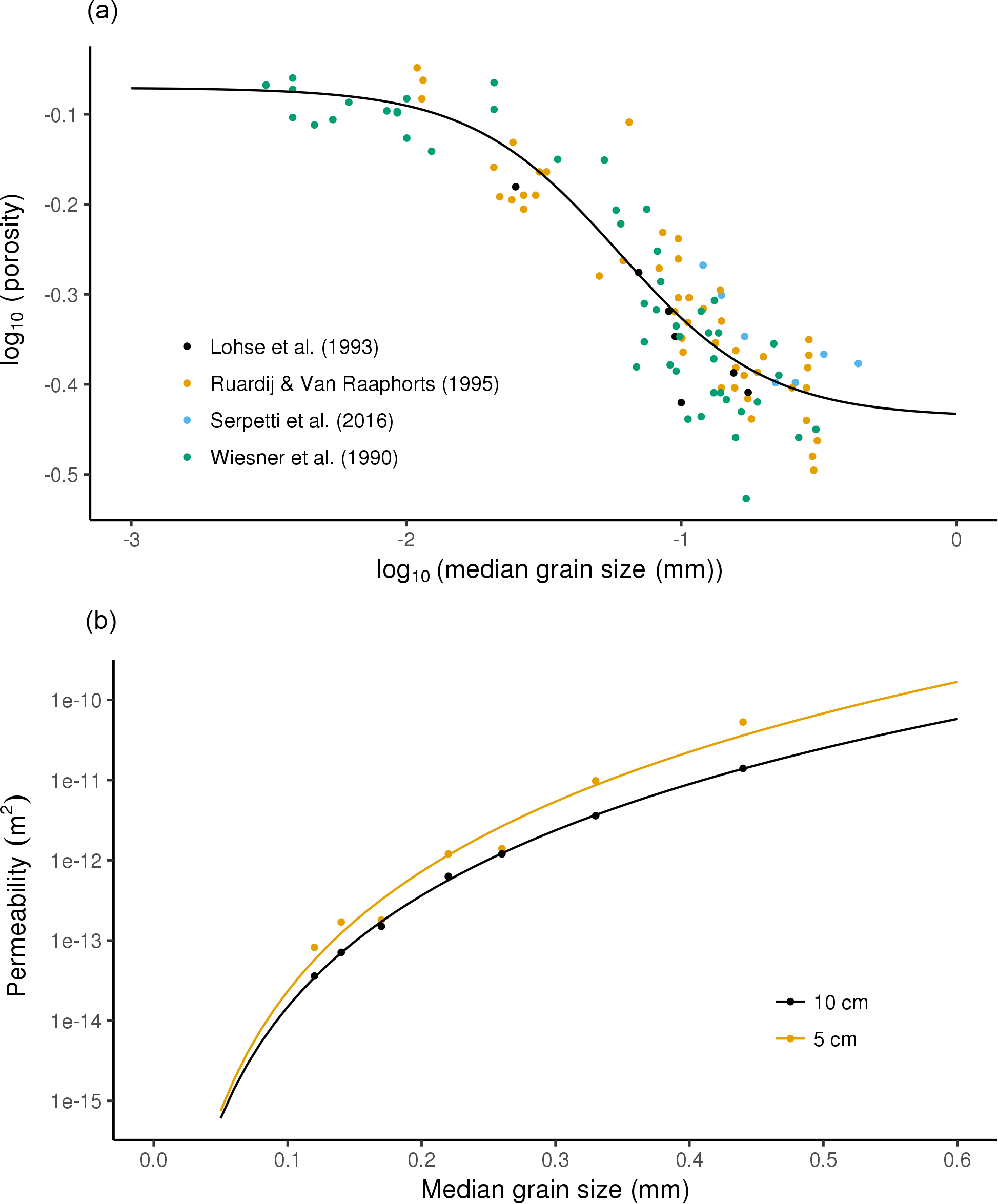
Figure 4(a) Assembled data on sediment porosity and median grain size (filled circles) and the fitted relationship (solid line). (b) Annual average permeability m−2 of sediments from seven sites off the north-east coast of Scotland; data from Serpetti et al. (2016).
2.3.2 Median grain sizes
Sufficient median grain size data were available to provide a spatial interpolation of whole-sediment D50 in most of the North Sea and large parts of the English Channel and Irish Sea. We therefore interpolated whole-sediment D50 in these regions. This was carried out in the same way as for the distribution of sediment percentages using bilinear spline interpolation and interpolating solely within the alphahull which surrounds the relevant data points. Outside the alphahulls we predict the relevant D50 using the mud, sand and gravel percentages in the synthetic maps created in this study.
In contrast to the mud, sand and gravel percentages, we chose not to predict median grain sizes using environmental variables. Predicting both the sediment percentages and median grain sizes separately is likely to result in contradictory predictions. For example, a model might predict a much higher median grain size than is possible given the predicted sediment percentages. We therefore chose to create a statistical model which predicts the median grain size using mud, sand and gravel percentages.
The median grain size of the gravel fraction has previously been shown to relate strongly to the mud to sand ratio (Aldridge et al., 2015). We therefore chose to model the whole-sediment D50, the sand D50 and the gravel D50 in relation to mud, sand and gravel percentages. In all cases we used general additive models (GAMs) (Wood, 2006), which marginally outperformed random forests in terms of predictive ability.
The median grain size of the whole sediment varied by 4 orders of magnitude. Consequently, a GAM which uses the D50 unaltered was incapable of credibly predicting the D50 for the small-grained muddy sediments. We therefore used the following log transformation for the general additive model of the total sediment median grain size; log10(D50)∼te(mud, sand, gravel), where the interactions between mud, sand and gravel percentages are accounted for using a tensor product smooth (te). As with the sediment percentages, data were split into training and testing data. We randomly selected 70 % of the data and used it as the training data, and then used the remaining 30 % as the test data. Likewise, the final predictive model was created using all of the data.
For the sand and gravel fractions we used a GAM of the form D50∼te(mud, sand, gravel), with a log-link function to ensure predictions were never negative. Finally, a small number of predictions for the sand and gravel D50 were outside the grain size boundaries for gravel or sand respectively. In these cases we forced the modelled D50 to be the largest or smallest possible grain size where appropriate. General additive models were created using the R package mgcv (Wood, 2001).
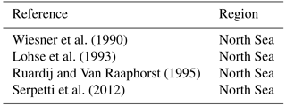
Wiesner et al. (1990)Lohse et al. (1993)Ruardij and Van Raaphorst (1995)Serpetti et al. (2012)Table 4Published literature with porosity estimates. These data were used to statistically model porosity in terms of whole-sediment median grain size.
2.3.3 Porosity and permeability
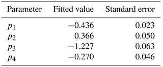
The porosity and permeability of sediments are quantitatively related to grain size distribution, with coarser-grained sediments having lower porosity and higher permeability. We evaluated the relationship between porosity and whole-sediment median grain size by compiling published data (Table 4). Porosity is conventionally expressed as the percentage volume of sediment occupied by void spaces of water. However, some data (Wiesner et al., 1990) expressed water percentage by weight. In this case we converted the water content data (by weight) to porosity assuming a solid material density of 2.65 g cm−3 and a fluid density of 1.025 g cm−3. There was a sigmoidal relationship between log-transformed porosity and log10 grain size (mm). We therefore fitted a logistic relationship between them using Nelder–Mead optimization in the optim package in R (Fig. 4). This equation is shown below and the parameters are given in Table 5.
To our knowledge the best dataset available on the relationship between whole-sediment permeability and median grain size is that of Serpetti et al. (2016). This dataset covered muddy sand, sand and mixed sediments sampled at approximately monthly intervals over 1 year at seven sites off the east coast of Scotland. Permeability and median grain size were measured on cores from the upper 5 cm and upper 10 cm of the seabed at each site. Most sediments are sampled at a depth of 10 cm and we therefore chose to only map permeability at this depth. The differences in annual average permeability (m−2) can be explained using a power function of median grain size (D50, mm) (r2=0.999 for 10 cm cores). The equation was as follows:
Porosity and permeability were mapped across the study region using the above equations and the synthetic map median grain size.
Table 5Fitted values and standard errors of the four parameters required for the function relating sediment porosity to median grain size.
We then used the porosity estimates and the maps of POC and TN to derive additional maps of the density of carbon (kg C m−2) and nitrogen (kg N m2) stored in the surface sediment layer across the shelf. This was derived from the carbon and nitrogen percentages of sediment and porosity values using the following equation.
2.3.4 Natural disturbance
We modelled the extent to which the surface layers of the sediment were disturbed by waves and tides during the year. Disturbance was defined as an event which results in physical movement of the surface sediments due to the effects of bed shear stress. We then estimated the average percentage of area disturbed per month in each 0.125∘ by 0.125∘ cell over our model region. We assumed that sediments are mobilized when the bed shear stress exceeds a critical Shields threshold and that this threshold is given by the equation provided by Wilcock et al. (2009).
Disturbance could be heterogeneous in space and time within each of our 0.125∘ by 0.125∘ cells due to variations in grain size and shear stress. We accounted for this heterogeneity as follows. The bed shear stress on the seabed is determined by the wave and tide conditions and the whole-sediment D50. However, for the mud, sand and gravel fraction the critical threshold is determined by the D50 of the relevant fraction.
We therefore estimate natural disturbance using the following procedure for each day of the year.
-
Calculate the bed shear stress at each 15 min time interval using equations shown in this paper's Appendix and the whole-sediment D50.
-
Determine the critical threshold at each time step for mud, sand and gravel using the respective D50 and Eq. (A50).
-
Percentage of area disturbed = (, where Muddist, Sanddist, Graveldist denote whether the Shields stress exceeded the critical threshold for mud, sand and gravel respectively.
We follow Aldridge et al. (2015) and use a 1-day time window to classify disturbance events. Monthly disturbance rates are then calculated by aggregating the areas disturbed in each day of the month. It is important to note that the modelled disturbance rate ignores the existence of rock at the surface. We are therefore only modelling the disturbance rate in regions with sediment cover.

Figure 5The derivation of the synthetic map of sediment percentages. The interpolated map uses bilinear spline interpolation using sediment data over the region. The random forest map predicts the sediment percentages using a random forest model which relates the percentage to the bed shear stress and the distance to the coast. The synthesized map merges the two by using spatial interpolations where we have data and the random forest predictions where we do not.
3.1 Sediment percentages and median grain sizes
Figure 5 shows the derivation of the synthetic map of sediment percentages. The interpolated map shows that mud (regions with greater than 50 % mud) is largely concentrated in the deep Norwegian Trench, an area in the north-western North Sea, part of the western Irish Sea and in patches on the Scottish west coast. Sandy sediments (greater than 50 % sand) dominate in the North Sea, except for those areas with high mud and a small region on the south-eastern English coast with high gravel levels. High gravel levels are seen exclusively in shallow coastal regions, with most of the English Channel having more than 50 % gravel.
The predictions of the random forest models reproduce the large-scale geographic patterns of sediment composition. The R2 values of the predictions of mean sediment percentage in each 0.125∘ by 0.125∘ grid cell on the test data were 0.444, 0.412 and 0.476 for mud, sand and gravel percentages respectively. The models pick up most of the key geographic features revealed by the spatially interpolated map. The high levels of mud in the Norwegian Trench, west of the Isle of Man and the region of the northern North Sea are reproduced. Regions of the western North Sea with relatively high mud levels are also well represented. Similarly, the model predicts the existence of relatively high levels of mud south of Ireland.
The GAM of whole-sediment D50 created using the training dataset performed well against the test data. R2 was 0.85 on the D50 values and 0.95 on the log10(D50) values. This model had an R2 of 0.98. Figure 6 shows the modelled relationship between percentages of mud, sand and gravel and the median grain size of the whole sediment. The GAM relating the sand D50 to the mud, sand and gravel percentages, which was trained on the training dataset, had an R2 0.42 when compared with the test data. The R2 for the GAM relating the gravel D50 to the mud, sand and gravel percentages was 0.38.
Figure 7 shows the derivation of the synthetic maps of median grain sizes. Whole-sediment median grain size can be interpolated for most of the North Sea, English Channel, and the Irish and Celtic seas. It varies by approximately 3 orders of magnitude, with median grain sizes above 10 mm in the gravelly regions in the English Channel and other coastal regions and median grain sizes close to 0.01 mm in muddy regions such as that in the north-western North Sea. The median grain size of the sand fraction can be interpolated for most British territorial waters and is highest in regions which are predominantly gravelly. The median grain size of the gravel fraction can only be interpolated for parts of southern British territorial waters, and it is highest in regions of high gravel content.
Figure 8 shows the derived maps of porosity and permeability. Porosity is similar across most regions, with the exception of the muddy areas in the Norwegian Trench, north-western North Sea and the Irish Sea. Permeability varies by 18 orders of magnitude. It is highest in the gravelly regions in the English Channel and some coastal regions, and it is lowest in muddy regions.
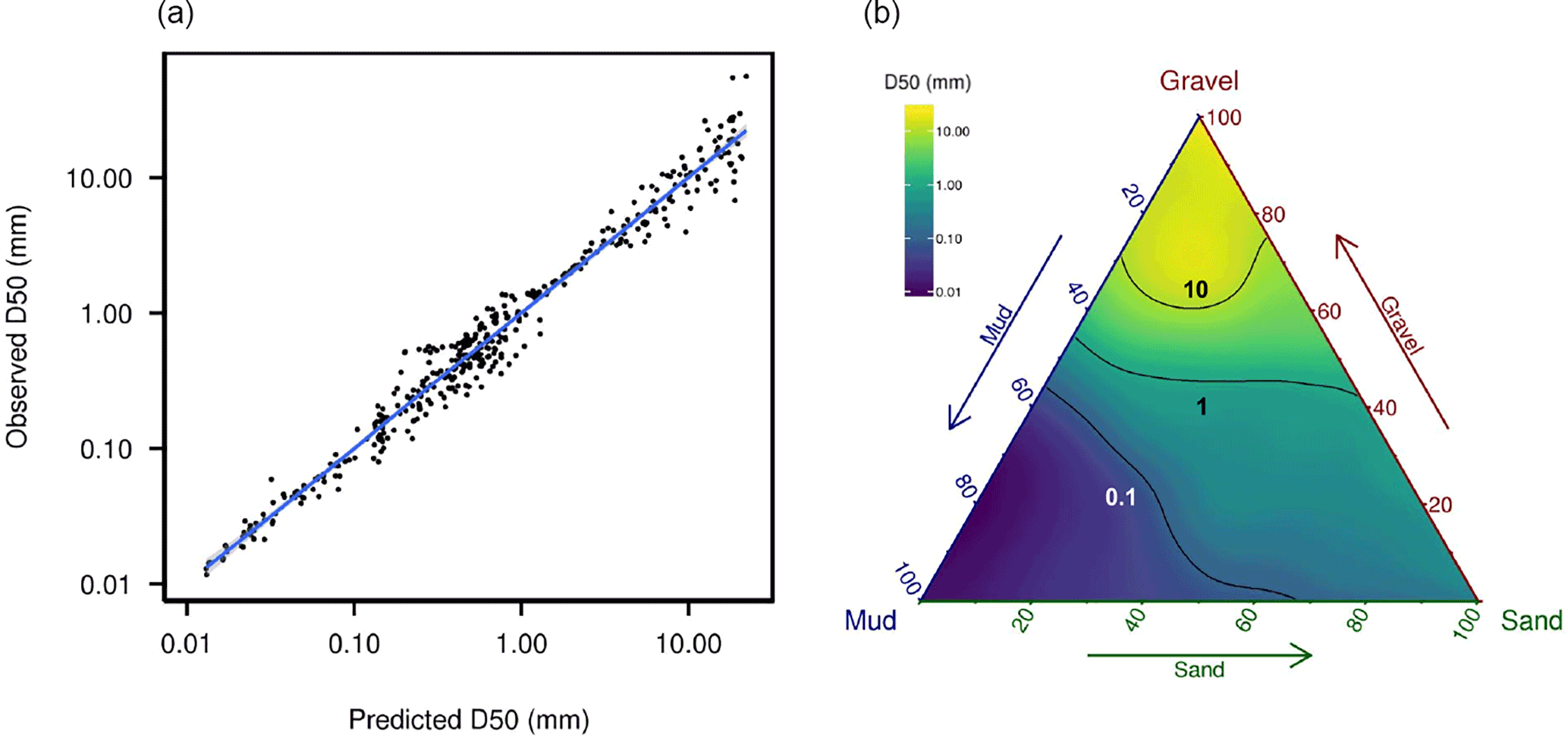
Figure 6(a) Predictions of a GAM that relates whole-sediment D50 to the mud, sand and gravel percentages. (b) Relationship between total sediment median grain size and percentage of mud, sand and gravel. The relationship was derived using a general additive model which relates the D50 to the mud, sand and gravel percentage.
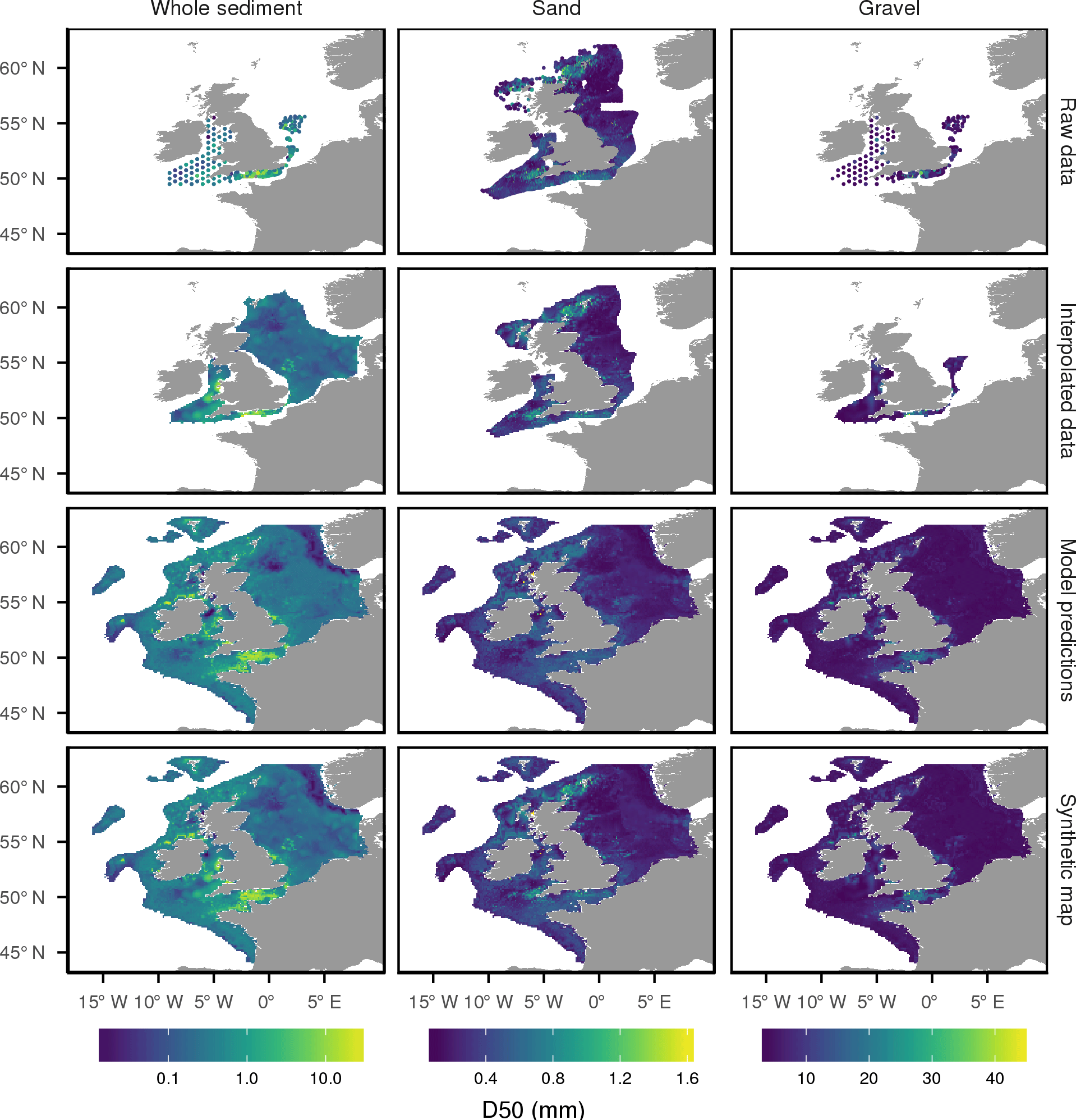
Figure 7Summary of the derivation of the synthetic median grain size maps. Where we have sufficient median grain size data we spatially interpolated a map of D50. In other locations we used the synthetic map of mud, sand and gravel percentages and a GAM which relates the D50 to the mud, sand and gravel percentages to predict the D50.
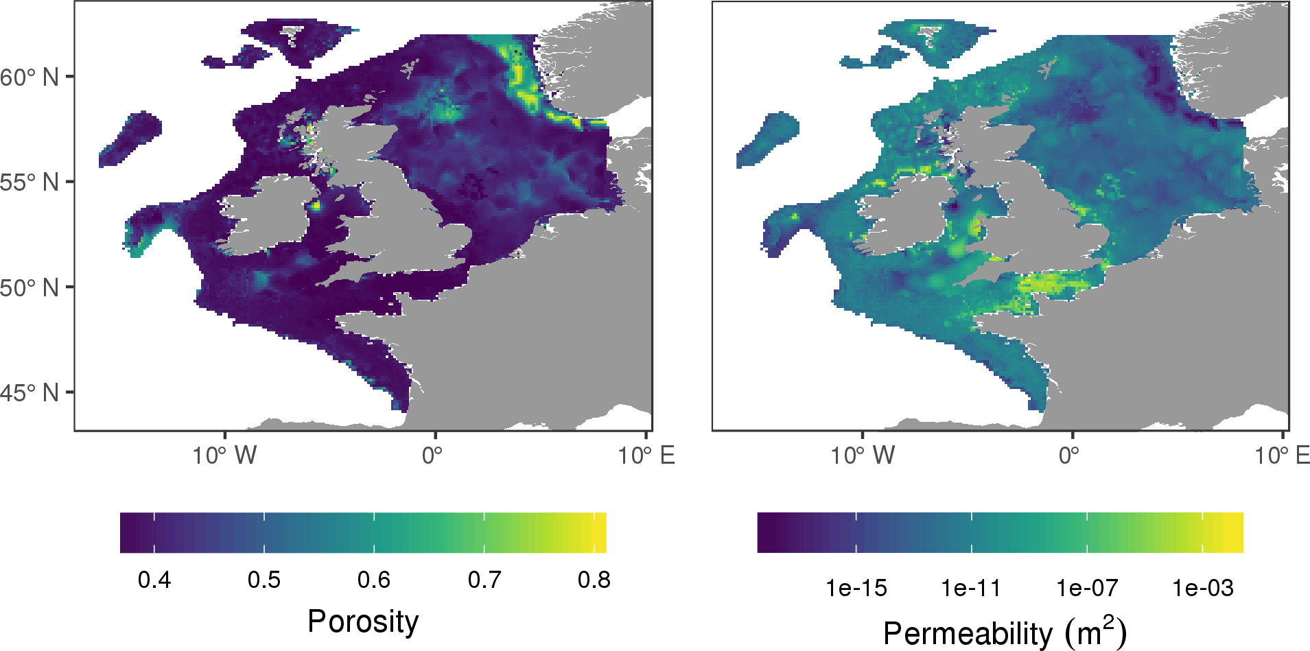
Figure 8Maps of porosity and permeability. The relationship between porosity and permeability and median grain size was estimated using published field data. We then predicted porosity and permeability using the synthetic map of median grain size.
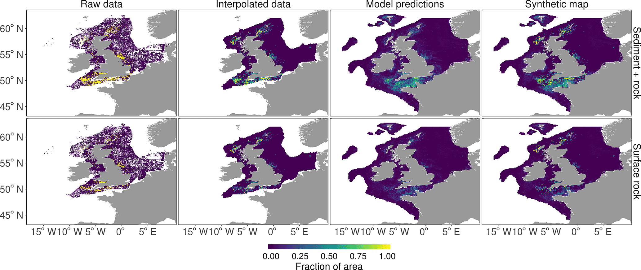
Figure 9Proportion of area in each rock classification. Areas were classified by whether there was rock at the surface or a surface sediment layer plus rock in the top 50 cm. Historical survey logs and borehole records were first interpolated to provide a map of rock cover where we have sufficient data. Random forests were used to predict rock cover elsewhere using wave and tidal velocities, bathymetry, measures of bathymetry variation and distance from the coast as predictors.
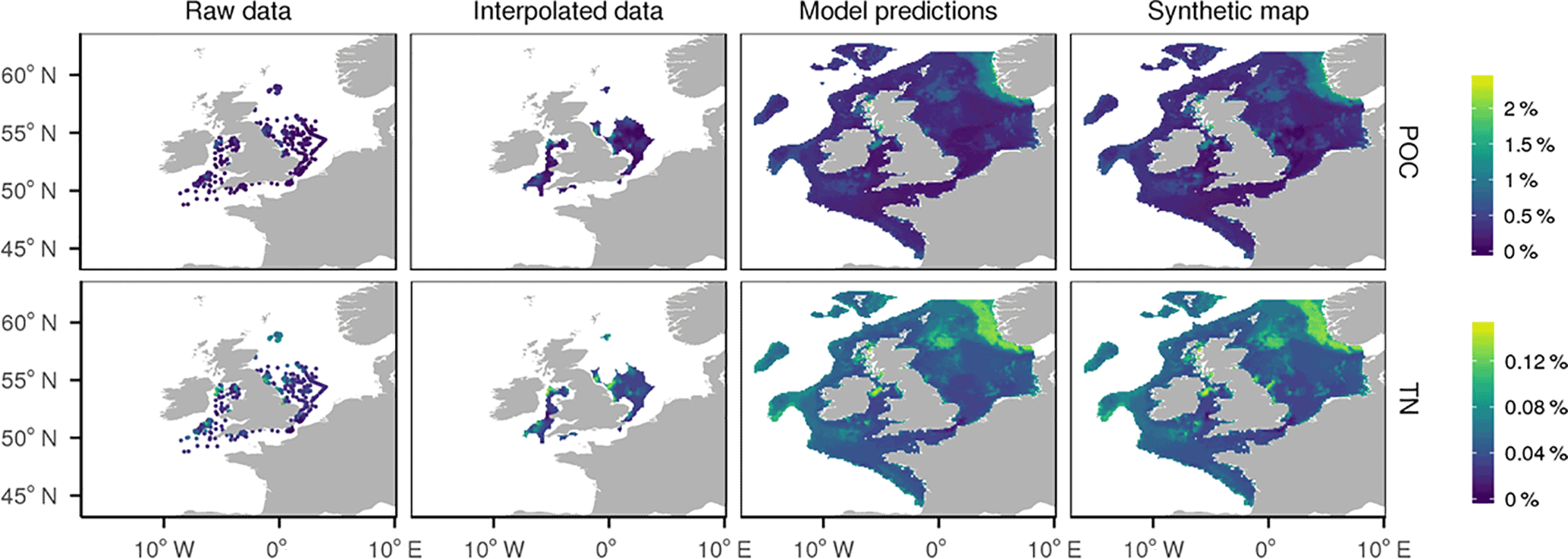
Figure 10Derivation of the synthetic maps of particulate organic carbon (POC) and nitrogen (TN). Data were interpolated based on field observations in areas with good spatial coverage. In other regions, parameters were predicted using a random forest which had mud content and physical environmental variables as predictors.
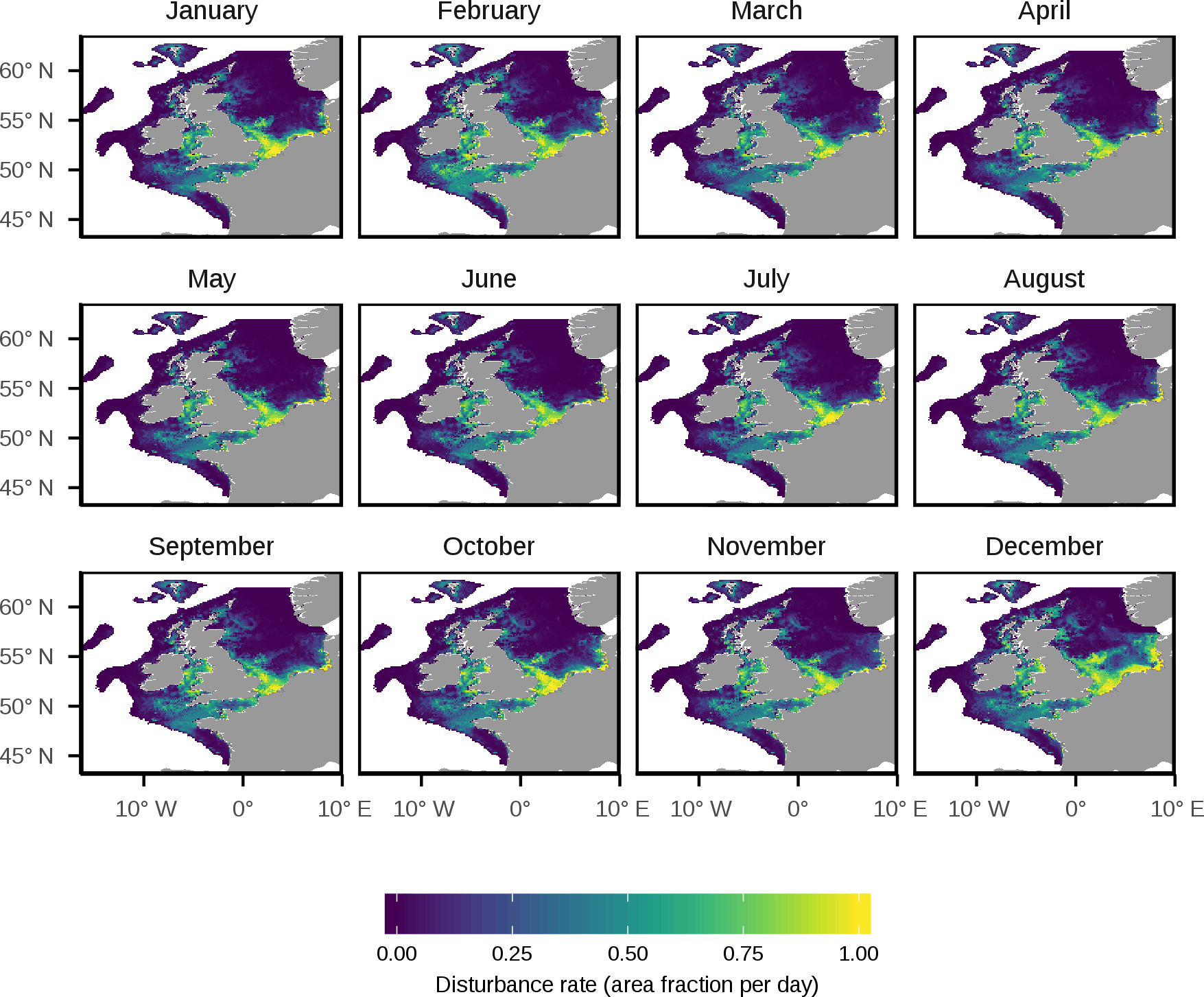
Figure 11Modelled monthly disturbance rate. A disturbance event was defined as a time when the bed shear stress exceeded the threshold required to move either the mud, sand or gravel portion of the sediment. The monthly disturbance rate was defined as the mean fraction of the total mud, sand and gravel area disturbed per day.
The synthetic maps of rock cover are shown in Fig. 9. Observed data indicate that the eastern North Sea is almost entirely free of surface rock. There are large concentrations of surface rock in the English Channel, south-west of England, the Bristol Channel and west of the Hebrides Islands on the west coast of Scotland. The predictions of the random forest model of rock provide credible large-scale reproductions of the geographic patterns of rock cover. Predictions of surface rock and rock in the top 50 cm have r2 of 0.104 and 0.1991 when compared with mean values in each 0.125∘ by 0.125∘ grid cell. The random forest predictions in Fig. 9 reproduce the key rock areas shown by the spatially interpolated map. Regions where we rely on predictions are largely rock free, with the notable exceptions of the high-energy English Channel, north-west of France and west of the Faroe Islands.
The mapped carbon and nitrogen content of sediment are shown in Fig. 10. The random forest predictions show close agreement with observations. Across 100 iterations in which training and test data were spatially disaggregated, 70 % of data in the training data, there was a mean r2 of 0.59 and 0.70 between predicted and observed POC and PON respectively. Carbon and nitrogen content are largely determined by mud content. Therefore the regions of high carbon and nitrogen content reflect those of large mud content.
3.2 Natural disturbance
Figure 11 shows modelled natural disturbance in each month. The deep Norwegian Trench is notable for lacking any disturbance year round. Disturbance is highest in the southern North Sea where sandy regions on the French, Belgian and Dutch coasts see disturbance events almost on a daily basis. There is a notable seasonal pattern in disturbance rates, with summer months seeing lower disturbance rates, which reflects the lower wind and wave regime in this time period.
The data products listed in Table 1 can been be downloaded in csv, netcdf and ESRI grid format from https://doi.org/10.15129/1e27b806-1eae-494d-83b5-a5f4792c46fc (Wilson et al., 2017).
The underlying goal of this study was to synthesize large-scale information about the physical environment of the seabed, both in terms of the characteristics of sediment and the wave and tidal regimes which cause disturbance. Using field estimates of the sediment composition of the seabed, we were able to map with high confidence the sediment composition of the North Sea and British territorial waters, and we were able to make credible statistical predictions of the sediment composition in other regions. The compiled datasets of sediment composition and disturbance regime are, as far as we know, the most extensive that exist over such a large spatial scale. A number of applications exist for these datasets, including habitat mapping and quantification of anthropogenic disturbance on the seabed.
Habitat mapping requires knowledge of the composition of seabed sediments (Galparsoro et al., 2012), and the maps we produced can be seen as complementary to previous work (e.g. the EU Mesh project; Vasquez et al., 2015). Existing habitat maps typically use discontinuous categories, and the continuous nature of the maps we have produced may be advantageous for some researchers.
Limitations and assumptions
A simplifying assumption of our study was that sedimentary environments are in a state of equilibrium or near equilibrium throughout the European Shelf. However, this is unlikely to be true everywhere. Ward et al. (2015) have argued that the coarser sediments found south-east of Ireland were inherited from prior stress regimes. Furthermore, the Irish Sea has linear tidal sand ridges, which are likely relics from an earlier more energetic stress regime (Uehara et al., 2006; Scourse et al., 2009). Reconstructions of historical tidal conditions on the European Shelf (e.g. Uehara et al., 2006; Neill et al., 2010, 2009) could potentially be included as model predictors in future modelling studies.
Our maps of rock area are broadly comparable with the existing hard substrate map for British territorial waters produced by the British Geological Survey (Gafeira et al., 2010). Both maps largely draw on historical British Geological Survey logs from sea-floor surveys; however, the philosophy and motivation of our study differed from that of the British Geological Survey. The British Geological Survey was motivated by mapping rocky reef areas for marine conservation planning purposes. Regions were classified as rock or non-rock, which inevitably leads to an overestimation of rock cover if analysts assume that all mapped rock regions are made up exclusively of rock. This is illustrated in the region west of the Hebrides Islands on the west coast of Scotland, where the British Geological Survey historical records show that the seabed is a complex mixture of rock-free seabed and rocky outcrops. However, the British Geological Survey substrate map classifies almost this entire area as rock. This classification was justifiable given the aim of identifying broad regions that may have rocky reefs. However, in applications such as species distribution modelling this approach is problematic. The classification of mixed habitats as rock could result in a priori ruling out a large amount of biological activity, such as fish spawning (Ellis et al., 2012), that is known to take place in these areas. In this case the continuous mapping approach taken by our study is likely more informative.
The confidence in our rock data products is significantly lower than that for mud, sand and gravel percentages. However, this was an expected result and was consistent with existing work (Diesing et al., 2015; Stephens and Diesing, 2015; Downie et al., 2016). The survey data we rely on were explicitly designed to estimate mud, sand and gravel percentages. In contrast, the rock data were based on interpretations of historical survey logs, which creates an additional level of uncertainty. Furthermore, our raw data revealed that rock cover shows large levels of heterogeneity. The low numbers of samples (1 or 2) available in most 0.125∘ by 0.125∘ grid cells means that our available estimates of rock cover are highly uncertain, which inevitably leads to a model with lower levels of predictability. Predictive modelling is also complex due to the array of conditions that appear to result in a rocky seabed. The English Channel and Bristol Channel are rocky due to the strong tidal energy regime, whereas the region west of the Hebrides Islands on the Scottish west coast is relatively rocky due to the existence of rocky outcrops. It is also possible that underlying geology plays a key role in determining rock levels. A previous study that took a similar predictive modelling approach in British waters used information about rock formations as predictors (Diesing et al., 2015; Downie et al., 2016); however, we were unable to find any comparable datasets that covered the entire north-west European Shelf.
We excluded the influence of rivers from predictive models because of a lack of large-scale data. However, it is likely that this is a key influence near large estuaries. This can be seen in the high-energy Bristol Channel, where there is both a high level of rock and a relatively high level of mud due to the contradictory influences of strong tidal currents and the sediment deposits from the river Severn (McLaren et al., 1993). The influence of river outflows is implicitly captured by the inclusion of distance from the coast as a predictor. For example, there is a large increase in the carbon content of sediments close to coasts, which is likely influenced by sediment deposits from rivers. We therefore cannot rule out the possibility that certain parameters were over- or under-predicted in coastal regions due to the influence of estuaries. Similarly, we did not include the potential effects of the horizontal transport of sediment by currents (Tiessen et al., 2017) or the cross-shore transport of wave-induced resuspended sediment due to the effects of gravity (Wright and Friedrichs, 2006; Falcini et al., 2012).
Previously, Aldridge et al. (2015) mapped the natural disturbance rates of the seabed in English territorial waters and a large part of the North Sea. Despite using different methodology and assumptions, our modelled disturbance rates were broadly similar for sandy and muddy regions. However, they deviated drastically for gravelly sediments, in particular in the English Channel. Our model typically predicted disturbance events to occur at least 10 times more often in gravelly sediments compared with Aldridge et al. (2015). This difference likely results from the assumption for median grain size. A key difference in assumptions between our work and Aldridge et al. (2015) is that we used the whole-sediment D50 as the basis for the bed roughness term in the shear stress and disturbance rate calculations, whereas Aldridge et al. (2015) used the D50 of the gravel fraction only. Where the seabed sediments are composed of mixtures of mud, sand and gravel fractions this leads to large differences in estimated disturbance rates. It is not clear which approach is more correct. The critical Shields stress calculations are parameterized from empirical studies of sorted sediments. The extent to which these calculations apply to poorly sorted sediments is uncertain. In fact, there is a lack of a theoretical and empirical basis for estimating the suspension and transport dynamics of sediments comprising mixtures of mud, sand and gravel. Sensitivity analysis (not shown) indicated that only using the gravel D50 to determine disturbance in our model resulted in comparable disturbance levels to those in Aldridge et al. (2015). Further research is therefore necessary to reduce the level of uncertainty in our knowledge of the disturbance of mixed coarse sediments.
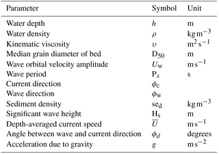
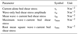
The bed shear stress and sediment dislocation rates were calculated by combining the equations of Soulsby and Clarke (2005), Soulsby (2006) and Wilcock et al. (2009).
Bed shear stress was calculated using the equations of Soulsby and Clarke (2005), who developed equations which calculate combined bed shear stress under waves and currents. Finally, we use the equations of Wilcock et al. (2009) to estimate the critical threshold required for the bed shear stress to cause dislocation of sediment from the sea floor. Model inputs and outputs are given in Tables A1 and A2 respectively.
A1 Calculation of wave orbital velocities
We calculate the wave orbital velocities using the equations of Soulsby (2006). All waves are assumed to be irregular (spectral).
The the zero-crossing period Tz (s), the peak period Tp (s) and the mean wave crossing period Tm (s) are calculated depending on whether there is a JONSWAP spectrum:
We calculate the natural scaling period, Tn, as follows:
Soulsby and Smallnan (1986) formulated equations which approximate the wave orbital velocity at the seabed, Uw ( m s−1), as follows.
where
and
A2 Intermediate calculations
We must then calculate a number of intermediate terms for the shear stress calculation.
We relate the kinematic viscosity υ (m2 s−1) to sea water density (1026.96 kg m−3) and kinematic velocity μ (kg (ms)−1).
If we define ϕc as the current direction and ϕw as the wave direction, then we can calculate ϕc as the angle between the current and wave direction as follows:
The bed roughness length, z0, is calculated as follows.
The Reynolds number for currents is calculated as
The current drag coefficient for smooth turbulent flow is calculated as follows:
The current drag coefficient for rough flow is calculated using the equation
The wave semi-orbital excursion is calculated using the equation
The Reynolds number for waves is calculated as follows:
The wave friction factor for smooth flow is calculated using the equation
The wave friction factor for rough flow is calculated using the equation
The bed shear stress depends on whether there are currents or waves only or whether there is a combination of waves and currents.
Case 1: and Uw=0; current only and no waves
The current-only shear stress is calculated as follows. When , we calculate the current bed shear stress under laminar flow equations.
When Rec>2000, we calculate the current bed shear stress under turbulent equations.
Case 4: and Uw>0; waves only, not currents
We calculate wave-only stress as follows.
4.1 Laminar flow:
Case 5: and Uw>0; combined wave and current flow
First we calculate the critical current Reynolds for transition from laminar to turbulent flow.
The critical wave Reynolds for transition from laminar to turbulent flow:
5.1 and
5.2 Turbulent flow: Rec>Rew or
We must recalculate τc and τw since it is possible that one or the other of these could appear as laminar flow when estimated independently. The following are for the current-only component of stress under combined wave and current turbulent conditions.
The following are for the wave-only component of stress under combined wave and current turbulent conditions.
5.2.1 Rough turbulent flow:
We calculate tmr and tmaxr as follows.
Shields number calculation
We calculate the bed shear velocity as
The Reynolds particle number is calculated as follows:
The Shields stress is calculated as
The critical Shields stress is calculated as follows from the empirical relationship shown in Wilcock et al. (2009).
Here there is a U-shaped relationship between grain size and the critical Shields stress because of the high stresses required to dislodge bigger grains and the cohesive nature of mud.
RMS shear stress for waves and currents
The root mean square shear stress is calculated as follows:
High-resolution versions of the paper's figures have been made available as a supplementary file so that figures can be used in presentations and reports.
The supplement related to this article is available online at: https://doi.org/10.5194/essd-10-109-2018-supplement.
The authors declare that they have no conflict of interest.
We thank John Aldridge (Cefas), Simon Greenstreet (Marine Scotland), Mike Robertson
(Marine Scotland) and Jennifer Valerius (Federal Maritime and
Hydrographic Agency, Germany) for providing access to sediment data. We are
grateful to Michela De Dominicis and Judith Wolf (National Oceanography
Centre, Liverpool) for providing outputs from the Scottish Shelf Model.
British Geological Survey data were provided under Open Government Licence
(contains British Geological Survey materials ©NERC). Valuable technical
support was provided by Ian Thurlbeck. This paper received funding under the
NERC Marine Ecosystem Programme (NE/L003120/1) and from the EPSRC TeraWatt
and EcoWatt projects (EP/J010170/1 and EP/K012851/1).
Edited by: Giuseppe M. R. Manzella
Reviewed by: two anonymous referees
Akima, H. and Gebhardt, A.: akima: Interpolation of Irregularly and Regularly Spaced Data, R package version 0.6-12, 2016. a
Aldridge, J. N., Parker, E. R., Bricheno, L. M., Green, S. L., and van der Molen, J.: Assessment of the physical disturbance of the northern European Continental shelf seabed by waves and currents, Cont. Shelf Res., 108, 121–140, https://doi.org/10.1016/j.csr.2015.03.004, 2015. a, b, c, d, e, f, g, h, i
Avelar, S., van der Voort, T. S., and Eglinton, T. I.: Relevance of carbon stocks of marine sediments for national greenhouse gas inventories of maritime nations, Carbon Balance Manag., 12, 10, https://doi.org/10.1186/s13021-017-0077-x, 2017. a
Bahn, V. and McGill, B. J.: Testing the predictive performance of distribution models, Oikos, 122, 321–331, https://doi.org/10.1111/j.1600-0706.2012.00299.x, 2013. a
Baretta, J. W., Ebenhöh, W., and Ruardij, P.: The European regional seas ecosystem model, a complex marine ecosystem model, Netherlands J. Sea Res., 33, 233–246, https://doi.org/10.1016/0077-7579(95)90047-0, 1995. a
Basford, D. and Eleftheriou, A.: The benthic environment of the North Sea (56∘ to 61∘ N), J. Mar. Biol. Assoc. UK, 68, 125–141, https://doi.org/10.1017/S0025315400050141, 1988. a
Basford, D. J., Eleftheriou, A., Davies, I. M., Irion, G., and Soltwedel, T.: The ICES North Sea benthos survey: the sedimentary environment, ICES J. Mar. Sci., 50, 71–80, 1993. a, b, c
BGS: BGS Legacy Particle Size Analysis uncontrolled data export, Tech. rep., British Geological Survey, 2013. a
Blackford, J. C.: An analysis of benthic biological dynamics in a North Sea ecosystem model, J. Sea Res., 38, 213–230, https://doi.org/10.1016/S1385-1101(97)00044-0, 1997. a
Breiman, L.: Random Forests, Mach. Learn., 45, 5–32, https://doi.org/10.1023/A:1010933404324, 2001. a, b
Bricheno, L. M., Wolf, J., and Aldridge, J.: Distribution of natural disturbance due to wave and tidal bed currents around the UK, Cont. Shelf Res., 109, 67–77, https://doi.org/10.1016/j.csr.2015.09.013, 2015. a
Canty, A. J.: Resampling methods in R: the boot package, R News, 2, 2–7, 2002. a
Cavalli, M., Tarolli, P., Marchi, L., and Dalla Fontana, G.: The effectiveness of airborne LiDAR data in the recognition of channel-bed morphology, Catena, 73, 249–260, https://doi.org/10.1016/j.catena.2007.11.001, 2008. a
De Dominicis, M., O'Hara Murray, R., and Wolf, J.: Multi-scale ocean response to a large tidal stream turbine array, Renewable Energ., 114, 1160–1179, https://doi.org/10.1016/j.renene.2017.07.058, 2017. a
Dee, D. P., Uppala, S. M., Simmons, A. J., Berrisford, P., Poli, P., Kobayashi, S., Andrae, U., Balmaseda, M. A., Balsamo, G., Bauer, P., Bechtold, P., Beljaars, A. C. M., van de Berg, L., Bidlot, J., Bormann, N., Delsol, C., Dragani, R., Fuentes, M., Geer, A. J., Haimberger, L., Healy, S. B., Hersbach, H., Hólm, E. V., Isaksen, L., Kållberg, P., Köhler, M., Matricardi, M., McNally, A. P., Monge-Sanz, B. M., Morcrette, J. J., Park, B. K., Peubey, C., de Rosnay, P., Tavolato, C., Thépaut, J. N., and Vitart, F.: The ERA-Interim reanalysis: Configuration and performance of the data assimilation system, Q. J. Roy. Meteor. Soc., 137, 553–597, https://doi.org/10.1002/qj.828, 2011. a
Diesing, M., Stephens, D., and Aldridge, J.: A proposed method for assessing the extent of the seabed significantly affected by demersal fishing in the Greater North Sea, ICES J. Mar. Sci., 70, 1085–1096, https://doi.org/10.1093/icesjms/fst048, 2013. a, b
Diesing, M., Green, S. L., Stephens, D., Lark, R. M., Stewart, H. A., and Dove, D.: Mapping seabed sediments: Comparison of manual, geostatistical, object-based image analysis and machine learning approaches, Cont. Shelf Res., 84, 107–119, https://doi.org/10.1016/j.csr.2014.05.004, 2014. a
Diesing, M., Green, S., Stephens, D., Cooper, R., and Mellett, C.: Semi-automated mapping of rock in the English Channel and Celtic Sea, JNCC Report 569, p. 19, 2015. a, b
Diesing, M., Kroger, S., Parker, R., Jenkins, C., Mason, C., and Weston, K.: Predicting the standing stock of organic carbon in surface sediments of the North-West European continental shelf, Biogeochemistry, 135, 183–200, https://doi.org/10.1007/s10533-017-0310-4, 2017. a, b
Downie, A. L., Diesing, R. K., and Cooper, S. L.: Semi-automated mapping of rock in the North Sea, JNCC Report 592, 2016. a, b
Eddelbuettel, D., François, R., Allaire, J., Chambers, J., Bates, D., and Ushey, K.: Rcpp: Seamless R and C++ integration, J. Stat. Softw., 40, 1–18, 2011. a
Edmonds, D. and Slingerland, R.: Significant effect of sediment cohesion on delta morphology, Nature Geosci., 3, 105–109, https://doi.org/10.1038/ngeo730, 2009. a
Egbert, G. D., Erofeeva, S. Y., and Ray, R. D.: Assimilation of altimetry data for nonlinear shallow-water tides: Quarter-diurnal tides of the Northwest European Shelf, Cont. Shelf Res., 30, 668–679, https://doi.org/10.1016/j.csr.2009.10.011, 2010. a
Ellis, J. R., Milligan, S. P., Readdy, L., Taylor, N., and Brown, M. J.: Spawning and nursery grounds of selected fish species in UK waters, Science Series Technical Report, 147, 56, 2012. a
Falcini, F. and Jerolmack, D. J.: A potential vorticity theory for the formation of elongate channels in river deltas and lakes, J. Geophys. Res.-Earth Surface, 115, 1–18, https://doi.org/10.1029/2010JF001802, 2010. a
Falcini, F., Fagherazzi, S., and Jerolmack, D. J.: Wave-supported sediment gravity flows currents: Effects of fluid-induced pressure gradients and flow width spreading, Cont. Shelf Res., 33, 37–50, https://doi.org/10.1016/j.csr.2011.11.004, 2012. a
Foden, J., Rogers, S. I., and Jones, A. P.: Human pressures on UK seabed habitats: a cumulative impact assessment, Mar. Ecol. Prog. Ser., 428, 33–47, 2011. a
Gafeira, J., Green, S., Dove, D., Morando, A., Cooper, R., Long, D., and Gatliff, R. W.: Developing the necessary data layers for Marine Conservation Zone selection – Distribution of rock / hard substrate on the UK Continental Shelf, Tech. rep., British Geological Survey, 2010. a, b
Galparsoro, I., Connor, D. W., Borja, Á., Aish, A., Amorim, P., Bajjouk, T., Chambers, C., Coggan, R., Dirberg, G., Ellwood, H., Evans, D., Goodin, K. L., Grehan, A., Haldin, J., Howell, K., Jenkins, C., Michez, N., Mo, G., Buhl-Mortensen, P., Pearce, B., Populus, J., Salomidi, M., Sánchez, F., Serrano, A., Shumchenia, E., Tempera, F., and Vasquez, M.: Using EUNIS habitat classification for benthic mapping in European seas: Present concerns and future needs, Mar. Pollut. Bull., 64, 2630–2638, https://doi.org/10.1016/j.marpolbul.2012.10.010, 2012. a
George, D. A. and Hill, P. S.: Wave climate, sediment supply and the depth of the sand-mud transition: A global survey, Mar. Geol., 254, 121–128, https://doi.org/10.1016/j.margeo.2008.05.005, 2008. a
Gray, J. S.: Species richness of marine soft sediments, Mar. Ecol. Prog. Ser., 244, 285–297, https://doi.org/10.3354/meps244285, 2002. a
Halpern, B. S., Walbridge, S., Selkoe, K. A., Kappel, C. V., Micheli, F., D'Agrosa, C., Bruno, J. F., Casey, K. S., Ebert, C., Fox, H. E., Fukita, R., Heinemann, D., Lenihan, H. S., Madin, E. M. P., Perry, M. T., Selig, E. R., Spalding, M., Steneck, R., and Watson, R.: A Global Map of Human Impact on Marine Ecosystems, Science, 319, 948–953, https://doi.org/10.1126/science.1149345, 2014. a
Hamilton, N.: ggtern: An Extension to `ggplot2', for the Creation of Ternary Diagrams, R package version 2.2.1, 2017. a
Heath, M. R.: Ecosystem limits to food web fluxes and fisheries yields in the North Sea simulated with an end-to-end food web model, Prog. Oceanogr., 102, 42–66, https://doi.org/10.1016/j.pocean.2012.03.004, 2012. a
Heath, M., Sabatino, A., Serpetti, N., McCaig, C., and O'Hara Murray, R.: Modelling the sensitivity of suspended sediment profiles to tidal current and wave conditions, Ocean Coast. Manage., 147, 49–66, https://doi.org/10.1016/j.ocecoaman.2016.10.018, 2016. a, b
Hijmans, R. J., Williams, E., and Vennes, C.: geosphere: Spherical Trigonometry. R package version 1.2–28, CRAN, R-project, org/package= geosphere, 2012. a
Huang, Z., Nichol, S. L., Siwabessy, J. P., Daniell, J., and Brooke, B. P.: Predictive modelling of seabed sediment parameters using multibeam acoustic data: a case study on the Carnarvon Shelf, Western Australia, International J. Geogr. Information Sci., 26, 283–307, https://doi.org/10.1080/13658816.2011.590139, 2012. a
James, G., Witten, D., Hastie, T., and Tibshirani, R.: An introduction to Statistical Learning, Springer, New York, https://doi.org/10.1007/978-1-4614-7138-7, 2013. a
Li, J., Heap, A. D., Potter, A., Huang, Z., and Daniell, J. J.: Can we improve the spatial predictions of seabed sediments? A case study of spatial interpolation of mud content across the southwest Australian margin, Cont. Shelf Res., 31, 1365–1376, https://doi.org/10.1016/j.csr.2011.05.015, 2011. a
Liaw, A. and Wiener, M.: Classification and Regression by randomForest, R news, 2, 18–22, https://doi.org/10.1177/154405910408300516, 2002. a, b
Loh, W.-Y.: Classification and regression trees, Wiley Interdisciplinary Reviews: Data Mining and Knowledge Discovery, 1, 14–23, https://doi.org/10.1002/widm.8, 2011. a
Lohse, L., Malschaert, J. F. P., Slomp, C. P., Helder, W., and Vanraaphorst, W.: Nitrogen cycling in North Sea sediments: interaction of denitrification and nitrification in offshore and coastal areas, Mar. Ecol. Prog. Ser., 101, 283–296, https://doi.org/10.3354/meps101283, 1993. a, b
McLaren, P., Collins, M. B., Gao, S., and Powys, R. I. L.: Sediment dynamics of the Severn Estuary and Inner Bristol Channel, J. Geol. Soc., 150, 589–603, https://doi.org/10.1144/gsjgs.150.3.0589, 1993. a
Neill, S. P., Scourse, J. D., Bigg, G. R., and Uehara, K.: Changes in wave climate over the northwest European shelf seas during the last 12,000 years, J. Geophys. Res., 114, C06015, https://doi.org/10.1029/2009JC005288, 2009. a
Neill, S. P., Scourse, J. D., and Uehara, K.: Evolution of bed shear stress distribution over the northwest European shelf seas during the last 12,000 years, Ocean Dynam., 60, 1139–1156, https://doi.org/10.1007/s10236-010-0313-3, 2010. a
Pateiro-López, B. and Rodríguez-Casal, A.: Generalizing the Convex Hull of a Sample: The R Package Alphahull, J. Stat. Softw., 34, 1–28, https://doi.org/10.18637/jss.v034.i05, 2010. a
Porter-Smith, R., Harris, P. T., Andersen, O. B., Coleman, R., Greenslade, D., and Jenkins, C. J.: Classification of the Australian continental shelf based on predicted sediment threshold exceedance from tidal currents and swell waves, Mar. Geol., 211, 1–20, https://doi.org/10.1016/j.margeo.2004.05.031, 2004. a
Roberts, D. R., Bahn, V., Ciuti, S., Boyce, M. S., Elith, J., Guillera-Arroita, G., Hauenstein, S., Lahoz-Monfort, J. J., Schroder, B., Thuiller, W., Warton, D. I., Wintle, B. A., Hartig, F., and Dormann, C. F.: Cross-validation strategies for data with temporal, spatial, hierarchical, or phylogenetic structure, Ecography, pp. 1–17, https://doi.org/10.1111/ecog.02881, 2017. a, b
Robinson, K. A., Ramsay, K., Lindenbaum, C., Frost, N., Moore, J., Wright, A. P., and Petrey, D.: Predicting the distribution of seabed biotopes in the southern Irish Sea, Cont. Shelf Res., 31, S120–S131, https://doi.org/10.1016/j.csr.2010.01.010, 2011. a
Ruardij, P. and Van Raaphorst, W.: Benthic nutrient regeneration in the ERSEM ecosystem model of the North Sea, Neth. J. Sea Res., 33, 453–483, https://doi.org/10.1016/0077-7579(95)90057-8, 1995. a, b, c
Scourse, J., Uehara, K., and Wainwright, A.: Celtic Sea linear tidal sand ridges, the Irish Sea Ice Stream and the Fleuve Manche: Palaeotidal modelling of a transitional passive margin depositional system, Mar. Geol., 259, 102–111, https://doi.org/10.1016/j.margeo.2008.12.010, 2009. a
Serpetti, N., Heath, M., Rose, M., and Witte, U.: High resolution mapping of sediment organic matter from acoustic reflectance data, Hydrobiologia, 680, 265–284, https://doi.org/10.1007/s10750-011-0937-4, 2012. a, b, c
Serpetti, N., Witte, U. F. M., and Heath, M. R.: Statistical modelling of variability in sediment-water nutrient and oxygen fluxes, Front. Earth Sci., 4, 1–17, https://doi.org/10.3389/feart.2016.00065, 2016. a, b
Soulsby, R.: Simplified calculation of wave orbital velocities, Tech. rep., HR Wallingford Ltd., Wallingford, 2006. a, b, c
Soulsby, R. L. and Clarke, S.: Bed shear-stresses under combined waves and currents on smooth and rough beds, HR Wallingford, Report TR137, 2005. a, b, c
Soulsby, R. L. and Smallnan, J. V.: A direct method of calculating bottom orbital velocity under waves, Tech. rep., Report SR76, Hydraulics Research Wallingford, 1986. a
Stephens, D. and Diesing, M.: Towards quantitative spatial models of seabed sediment composition, PLoS ONE, e0142502, https://doi.org/10.1371/journal.pone.0142502, 2015. a, b, c, d
Thrush, S. F., Hewitt, J. E., Norkko, A., Nicholls, P. E., Funnell, G. A., and Ellis, J. I.: Habitat change in estuaries: Predicting broad-scale responses of intertidal macrofauna to sediment mud content, Mar. Ecol. Prog. Ser., 263, 101–112, https://doi.org/10.3354/meps263101, 2003. a
Tiessen, M. C., Eleveld, M. A., Nauw, J. J., Nechad, B., and Gerkema, T.: Depth dependence and intra-tidal variability of Suspended Particulate Matter transport in the East Anglian plume, J. Sea Res., 127, 2–11, https://doi.org/10.1016/j.seares.2017.03.008, 2017. a
Uehara, K., Scourse, J. D., Horsburgh, K. J., Lambeck, K., and Purcell, A. P.: Tidal evolution of the northwest European shelf seas from the Last Glacial Maximum to the present, J. Geophys. Res.-Oceans, 111, 1–15, https://doi.org/10.1029/2006JC003531, 2006. a, b
Valerius, J., V., V. L., S., V. H., Let, J. O., and Zeiler, M.: Trans-national database of North Sea sediment data. Data compilation by Federal Maritime and Hydrographic Agency (Germany); Royal Belgian Institute of Natural Sciences (Belgium); TNO (Netherlands) and Geological Survey of Denmark and Greenland (Denmark)., Tech. rep., 2015. a, b
VanDerWal, J., Falconi, L., Januchowski, S., Shoo, L., and Storlie, C.: SDMTools: Species Distribution Modelling Tools: Tools for processing data associated with species distribution modelling exercises, R package version 1.1-221, 2014. a
Vasquez, M., Mata Chacón, D., Tempera, F., O'Keeffe, E., Galparsoro, I., Sanz Alonso, J. L., Gonçalves, J. M. S., Bentes, L., Amorim, P., Henriques, V., McGrath, F., Monteiro, P., Mendes, B., Freitas, R., Martins, R., and Populus, J.: Broad-scale mapping of seafloor habitats in the north-east Atlantic using existing environmental data, J. Sea Res., 100, 120–132, https://doi.org/10.1016/j.seares.2014.09.011, 2015. a, b, c
Ward, S. L., Neill, S. P., Van Landeghem, K. J. J., and Scourse, J. D.: Classifying seabed sediment type using simulated tidal-induced bed shear stress, Mar. Geol., 367, 94–104, https://doi.org/10.1016/j.margeo.2015.05.010, 2015. a, b, c
Wessel, P. and Smith, W. H. F.: A global, self-consistent, hierarchical, high-resolution shoreline, J. Geophys. Res., 101, 8741–8743, 1996. a
Wickham, H.: ggplot2: elegant graphics for data analysis, Springer, New York, 2016. a
Wickham, H., Francois, R., Henry, L., and Müller, K.: dplyr: A Grammar of Data Manipulation, R package version 0.7.0, 2017. a
Wiesner, M. G., Haake, B., and Wirth, H.: Organic facies of surface sediments in the North Sea, Org. Geochem., 15, 419–432, https://doi.org/10.1016/0146-6380(90)90169-Z, 1990. a, b
Wilcock, P. R., Pitlick, J., and Cui, Y.: Sediment transport primer, estimating bed-material transport in gravel-bed rivers. Gen Tech Rep RMRS-GTR-226, Tech. rep., US Department of Agriculture, Forest service, Rocky Mountain Research Station: Fort Collins, CO, 78, 2009. a, b, c, d
Wilson, M. F. J., O'Connell, B., Brown, C., Guinan, J. C., and Grehan, A. J.: Multiscale Terrain Analysis of Multibeam Bathymetry Data for Habitat Mapping on the Continental Slope, Marine Geodysy., 30, 3–35, https://doi.org/10.1080/01490410701295962, 2007. a
Wilson, R., Heath, M., Speirs, D., and Sabatino, A.: Data for: “A synthetic map of the northwest European Shelf sedimentary environment for applications in marine science”, available at: https://doi.org/10.15129/1e27b806-1eae-494d-83b5-a5f4792c46fc, last access: 8 November 2017.
Wood, S. N.: mgcv: GAMs and generalized ridge regression for R, R News, 1, 20–25, https://doi.org/10.1159/000323281, 2001. a
Wood, S. N.: Generalized Additive Models: an introduction with R, Chapman and Hall, London, https://doi.org/10.1111/j.1541-0420.2007.00905_3.x, 2006. a
Wright, L. D. and Friedrichs, C. T.: Gravity-driven sediment transport on continental shelves: A status report, Cont. Shelf Res., 26, 2092–2107, https://doi.org/10.1016/j.csr.2006.07.008, 2006. a
Wright, M. N. and Ziegler, A.: ranger: A Fast Implementation of Random Forests for High Dimensional Data in C++ and R, J. Stat. Softw., 77, https://doi.org/10.18637/jss.v077.i01, 2017. a