the Creative Commons Attribution 4.0 License.
the Creative Commons Attribution 4.0 License.
 | 11 Jun 2024
Global nitrous oxide budget (1980–2020)
Naiqing Pan
Rona L. Thompson
Josep G. Canadell
Parvadha Suntharalingam
Pierre Regnier
Eric A. Davidson
Michael Prather
Philippe Ciais
Marilena Muntean
Shufen Pan
Wilfried Winiwarter
Sönke Zaehle
Feng Zhou
Robert B. Jackson
Hermann W. Bange
Sarah Berthet
Zihao Bian
Daniele Bianchi
Alexander F. Bouwman
Erik T. Buitenhuis
Geoffrey Dutton
Minpeng Hu
Akihiko Ito
Atul K. Jain
Aurich Jeltsch-Thömmes
Fortunat Joos
Sian Kou-Giesbrecht
Paul B. Krummel
Angela Landolfi
Ronny Lauerwald
Ya Li
Chaoqun Lu
Taylor Maavara
Manfredi Manizza
Dylan B. Millet
Jens Mühle
Prabir K. Patra
Glen P. Peters
Xiaoyu Qin
Peter Raymond
Laure Resplandy
Judith A. Rosentreter
Daniele Tonina
Francesco N. Tubiello
Guido R. van der Werf
Nicolas Vuichard
Junjie Wang
Kelley C. Wells
Luke M. Western
Chris Wilson
Jia Yang
Yuanzhi Yao
Yongfa You
Qing Zhu
Nitrous oxide (N2O) is a long-lived potent greenhouse gas and stratospheric ozone-depleting substance that has been accumulating in the atmosphere since the preindustrial period. The mole fraction of atmospheric N2O has increased by nearly 25 % from 270 ppb (parts per billion) in 1750 to 336 ppb in 2022, with the fastest annual growth rate since 1980 of more than 1.3 ppb yr−1 in both 2020 and 2021. According to the Sixth Assessment Report of the Intergovernmental Panel on Climate Change (IPCC AR6), the relative contribution of N2O to the total enhanced effective radiative forcing of greenhouse gases was 6.4 % for 1750–2022. As a core component of our global greenhouse gas assessments coordinated by the Global Carbon Project (GCP), our global N2O budget incorporates both natural and anthropogenic sources and sinks and accounts for the interactions between nitrogen additions and the biogeochemical processes that control N2O emissions. We use bottom-up (BU: inventory, statistical extrapolation of flux measurements, and process-based land and ocean modeling) and top-down (TD: atmospheric measurement-based inversion) approaches. We provide a comprehensive quantification of global N2O sources and sinks in 21 natural and anthropogenic categories in 18 regions between 1980 and 2020. We estimate that total annual anthropogenic N2O emissions have increased 40 % (or 1.9 Tg N yr−1) in the past 4 decades (1980–2020). Direct agricultural emissions in 2020 (3.9 Tg N yr−1, best estimate) represent the large majority of anthropogenic emissions, followed by other direct anthropogenic sources, including fossil fuel and industry, waste and wastewater, and biomass burning (2.1 Tg N yr−1), and indirect anthropogenic sources (1.3 Tg N yr−1) . For the year 2020, our best estimate of total BU emissions for natural and anthropogenic sources was 18.5 (lower–upper bounds: 10.6–27.0) Tg N yr−1, close to our TD estimate of 17.0 (16.6–17.4) Tg N yr−1. For the 2010–2019 period, the annual BU decadal-average emissions for both natural and anthropogenic sources were 18.2 (10.6–25.9) Tg N yr−1 and TD emissions were 17.4 (15.8–19.20) Tg N yr−1. The once top emitter Europe has reduced its emissions by 31 % since the 1980s, while those of emerging economies have grown, making China the top emitter since the 2010s. The observed atmospheric N2O concentrations in recent years have exceeded projected levels under all scenarios in the Coupled Model Intercomparison Project Phase 6 (CMIP6), underscoring the importance of reducing anthropogenic N2O emissions. To evaluate mitigation efforts and contribute to the Global Stocktake of the United Nations Framework Convention on Climate Change, we propose the establishment of a global network for monitoring and modeling N2O from the surface through to the stratosphere. The data presented in this work can be downloaded from https://doi.org/10.18160/RQ8P-2Z4R (Tian et al., 2023).
- Article
(24211 KB) - Full-text XML
-
Supplement
(1263 KB) - BibTeX
- EndNote


The global N2O budget has been perturbed through direct and indirect anthropogenic emissions as well as through perturbations to the natural N2O sources and sinks via climate change, increasing atmospheric CO2, and land-cover change. Ice core data show a relatively constant tropospheric N2O mixing ratio over the past 2 millennia (Canadell et al., 2021; MacFarling Meure et al., 2006; Fischer et al., 2019), followed by an increase from about 270 ppb (parts per billion) in 1750 to well above 300 ppb in the 2010s. The tropospheric N2O mole fractions, precisely measured at a global network of stations, increased from 301 ppb in 1980 to 333 ppb in 2020 and 336 ppb in 2022. The tropospheric N2O mole fraction in 2022 is higher than at any time in the last 800 000 years. The current growth rate of atmospheric N2O is unprecedented with respect to the ice core record covering the last deglacial transition (with decadal to centennial resolution) and likely unprecedented relative to the ice core records of the past 800 000 years. The mean annual tropospheric growth rate increased from 0.76 (lower–upper bounds: 0.55–0.95) ppb yr−1 in the decade from 2000 to 2009 to 0.96 (0.79–1.15) ppb yr−1 in the decade from 2010 to 2019. In 2020, the N2O tropospheric growth rate was 1.33 ppb yr−1 (1.38 ppb yr−1 in 2021), the highest observed rate since 1980 and over 30 % higher than the average in the 2010s.
Global N2O emissions have significantly increased in the last 4 decades. The magnitudes of global N2O emissions estimated by the bottom-up (BU) and top-down (TD) approaches were comparable during the overlapping period from 1997 to 2020, but TD estimates found a larger interannual variability and a faster rate of increase. BU approaches estimated that global N2O emissions increased from 17.4 Tg N yr−1 (10.3–24.0 Tg N yr−1) in 1997 to 18.5 Tg N yr−1 (10.6–27.0 Tg N yr−1) in 2020, with an average increase rate of 0.043 Tg N yr−2 (p<0.05). In contrast, according to TD estimates, global emissions increased from 15.4 Tg N yr−1 (13.9–16.7 Tg N yr−1) in 1997 to 17.0 Tg N yr−1 (16.6–17.4 Tg N yr−1) in 2020, implying a higher increase rate of 0.085 Tg N yr−2 (p<0.05).
According to BU estimates, the increase in global N2O emissions was primarily due to a 40 % increase in anthropogenic emissions from 4.8 (3.1–7.3) Tg yr−1 in 1980 to 6.7 (3.3–10.9) Tg yr−1 in 2020. Among all anthropogenic sources, direct agricultural emissions made the largest contribution, increasing from 2.2 (1.6–2.8) Tg N yr−1 in 1980 to 3.9 (2.9–5.1) Tg N yr−1 in 2020. The concurrent indirect agricultural N2O emissions also steadily increased from 0.9 (0.7–1.1) to 1.3 (0.9–1.6) Tg N yr−1. In contrast, other direct anthropogenic emissions (including emissions from fossil fuel and industry, biomass burning, and waste and wastewater) did not show a significant trend, while fluxes induced by perturbations to climate, atmospheric CO2, and land cover were negative and caused a reduction in N2O emissions that grew from −0.4 (−0.9 to 1.0) Tg yr−1 in 1980 to −0.6 (−2.2 to 1.8) Tg yr−1 in 2020. Unlike anthropogenic emissions, global natural land and ocean N2O emissions were relatively stable. According to the BU approaches, the total amount of global natural N2O emissions fluctuated between 11.7 and 12.1 Tg yr−1 during 1980–2020. Among all sources, natural emissions from shelves, inland waters, and lightning and atmospheric production were assumed to be constant during 1980–2020. According to BU approaches, the total natural emissions from these sources were 1.8 (1.0–3.0) Tg N yr−1.

Figure 1Global N2O budget during 2010–2019. The colored arrows represent N2O fluxes (in Tg N yr−1 for 2010–2019) as follows: red – direct emissions from nitrogen additions in the agricultural sector (agriculture); orange – emissions from other direct anthropogenic sources; maroon – indirect emissions from anthropogenic nitrogen additions; brown – perturbed fluxes from changes in climate, CO2, or land cover; and green – emissions from natural sources. The anthropogenic and natural N2O sources are derived from BU estimates. The blue arrows represent the surface sink and the observed atmospheric chemical sink, about 1 % of which occurs in the troposphere. The total budget (sources + sinks) does not exactly match the observed atmospheric accumulation, as each of the terms has been derived independently and we do not force TD agreement by rescaling the terms. This imbalance falls within the overall uncertainty in closing the N2O budget, as reflected in each of the terms. The N2O sources and sinks are given in teragrams of nitrogen per year (Tg N yr−1). © The Global Carbon Project.
During 2010–2019, similar estimates of global total N2O emissions were obtained using both the BU and TD approaches, with decadal mean values of 18.2 (10.6–25.9) Tg N yr−1 and 17.4 (15.8–19.2) Tg N yr−1, respectively (Fig. 1). According to the BU estimates, natural sources contributed 65 % to the total emissions (11.8, 7.3–15.9 Tg N yr−1). Specifically, natural soils contributed the most, with a decadal average of 6.4 (3.9–8.6) Tg N yr−1, followed by open oceans (3.5, 2.5–4.7 Tg N yr−1), the natural source from shelves (1.2, 0.6–1.6 Tg N yr−1), lightning and atmospheric production (0.6, 0.3–1.2 Tg N yr−1), and inland waters, estuaries, and coastal vegetation (0.1, 0.0–0.1 Tg N yr−1). Anthropogenic sources contributed 35 % to the total N2O emissions (6.5, 3.2–10.0 Tg N yr−1). Direct agricultural emissions accounted for 56 % of the total anthropogenic emissions (3.6, 2.7–4.8 Tg N yr−1), followed by emissions from other direct anthropogenic sources (2.1, 1.8–2.4 Tg N yr−1), including fossil fuel and industry (1.1, 1.0–1.2 Tg N yr−1), waste and wastewater (0.3, 0.3–0.3 Tg N yr−1), and biomass burning (0.8, 0.5–1.0 Tg N yr−1), and indirect anthropogenic emissions (1.2, 0.9–1.6 Tg N yr−1). Perturbed fluxes from climate, CO2, and land-cover changes had a net negative effect (i.e., reduced) on N2O emissions (−0.6, −2.1 to 1.2 Tg N yr−1). Increased CO2 and land conversion from mature forest reduced N2O emissions, but climate change resulted in N2O emission of 0.7 (0.2–1.2) Tg N yr−1.
Among the 18 regions considered in this study, only Europe, Russia, Australasia, and Japan and Korea had decreasing N2O emissions. Europe had the largest rate of decrease, with an average of Tg N yr−2 during 1980–2020 (31 % reduction), largely resulting from reduced fossil fuel and industry emissions, which changed from 0.49 Tg N yr−1 in 1980 to 0.14 Tg N yr−1 in 2020. In addition to the large reduction in fossil fuel and industry emissions in Europe, direct and indirect agricultural emissions also declined during 1980–2020; however, the decreasing trend in direct agricultural emissions had leveled off by the 2000s.
China and South Asia had the largest increases in N2O emissions from 1980 to 2020. The rates of increase in anthropogenic emissions from China and South Asia were Tg N yr−2 (82 % increase) and Tg N yr−2 (92 % increase), respectively. In these two regions, direct nitrogen additions in agriculture made the largest contribution, while other direct and indirect emissions also steadily increased.
The atmospheric chemistry transport models used in this study show an increase in the atmospheric N2O burden, from 1527 (1504–1545) Tg N in 2000–2009 to 1606 (1592–1621) Tg N in 2020, and, proportional to this, a small increase in the atmospheric loss, from 12.1 (12.0–12.6) to 12.9 (12.5–13.2) Tg N yr−1. The estimated increase in the atmospheric N2O burden is comparable to estimates by satellite and photolysis models, showing an increase from 1528 Tg N in the 2000s to 1570 Tg N in the 2010s and 1592 Tg N in 2020. The atmospheric chemistry transport models, however, did not show any significant trend in the lifetime, which is in contrast to results based on satellite observations in the stratosphere; these observations indicate that the atmospheric lifetime of N2O decreased from 119 years in the 2000s to 117 years in the 2010s. The reason for the discrepancy is not yet known and needs to be further investigated.
The following major uncertainties have been identified:
-
Inversion estimates are the most uncertain in the areas of South America, Africa, central and southern Asia, and Australasia, where the inversions are poorly constrained by observations.
-
Large uncertainties exist in the estimates of soil N2O emissions from tropical ecosystems in the Amazon Basin, the Congo Basin, and Southeast Asia as well as in regions with high fertilizer application rates and emissions, including eastern China, northern India, and the US Corn Belt.
-
The largest uncertainties in the estimates of ocean emissions are found in the equatorial Pacific, the Benguela upwelling region of the Atlantic, and the eastern equatorial Indian Ocean. The highest uncertainty in the equatorial upwelling and low-oxygen waters is associated with high subsurface N2O production.
-
The N2O fluxes from atmospheric CO2, mature forest conversion, and biomass burning are poorly understood and quantified. The relatively sparse distribution of current N2O observation sites underscores the necessity to establish more sites and regular aircraft profiles, especially in tropical and subtropical regions, to better constrain emission estimates from inversion models.
Based on this analysis and associated uncertainties, we propose the urgent development of a comprehensive terrestrial and ocean N2O flux monitoring and analysis network to better resolve spatiotemporal patterns and reduce uncertainties in N2O emissions. Such a development is a requirement to better constrain the future contribution of N2O to climate change and guide policy choices to reduce N2O emissions.
Nitrogen (N) is an essential element for the survival of all living organisms and is required by numerous biological molecules such as nucleic acids, proteins, and chlorophyll (Galloway et al., 2021; Scheer et al., 2020). The addition of excess reactive N compounds to terrestrial and oceanic ecosystems stimulates emissions of nitrous oxide (N2O), which is the most important depleting substance of stratospheric ozone (World Meteorological Organization, 2022) and a long-lived potent greenhouse gas with an atmospheric lifetime of more than 100 years (Myhre et al., 2013; Prather et al., 2015). Atmospheric N2O mole fractions have increased by nearly 25 % since the preindustrial era, from 270 ppb (parts per billion) in 1750 (MacFarling Meure et al., 2006) to 336 ppb in 2022, and have shown an increase of 35 ppb (10 %) since 1980 (Fig. 2). The current mole fraction is higher than at any time in the last 800 000 years (Schilt et al., 2010). The increase rate of atmospheric N2O in the 20th century is unprecedented over the past 20 000 years, covering the last glacial–interglacial transition, and likely unprecedented compared to the lower-resolution ice core records of the past 800 000 years (Joos and Spahni, 2008; Schilt et al., 2010; Canadell et al., 2021 AR6, WGI, Chap. 5). The observation networks of the Advanced Global Atmospheric Gases Experiment (AGAGE; Prinn et al., 2018), the National Ocean and Atmospheric Administration (NOAA; Hall et al., 2007), and the Commonwealth Scientific and Industrial Research Organization (CSIRO; Francey et al., 2003) all show an overall increasing trend in the growth rate of atmospheric N2O: the mean annual growth rate increased from 0.76 (0.55–0.95) ppb yr−1 in the 2000s to 0.96 (0.79–1.15) ppb yr−1 in the 2010s, with significant seasonal and interannual variation. In 2020, the N2O atmospheric growth rate was 1.33 ppb yr−1 (1.38 ppb yr−1 in 2021), higher than any previous observed year, and more than 30 % higher than the average value in the 2010s.
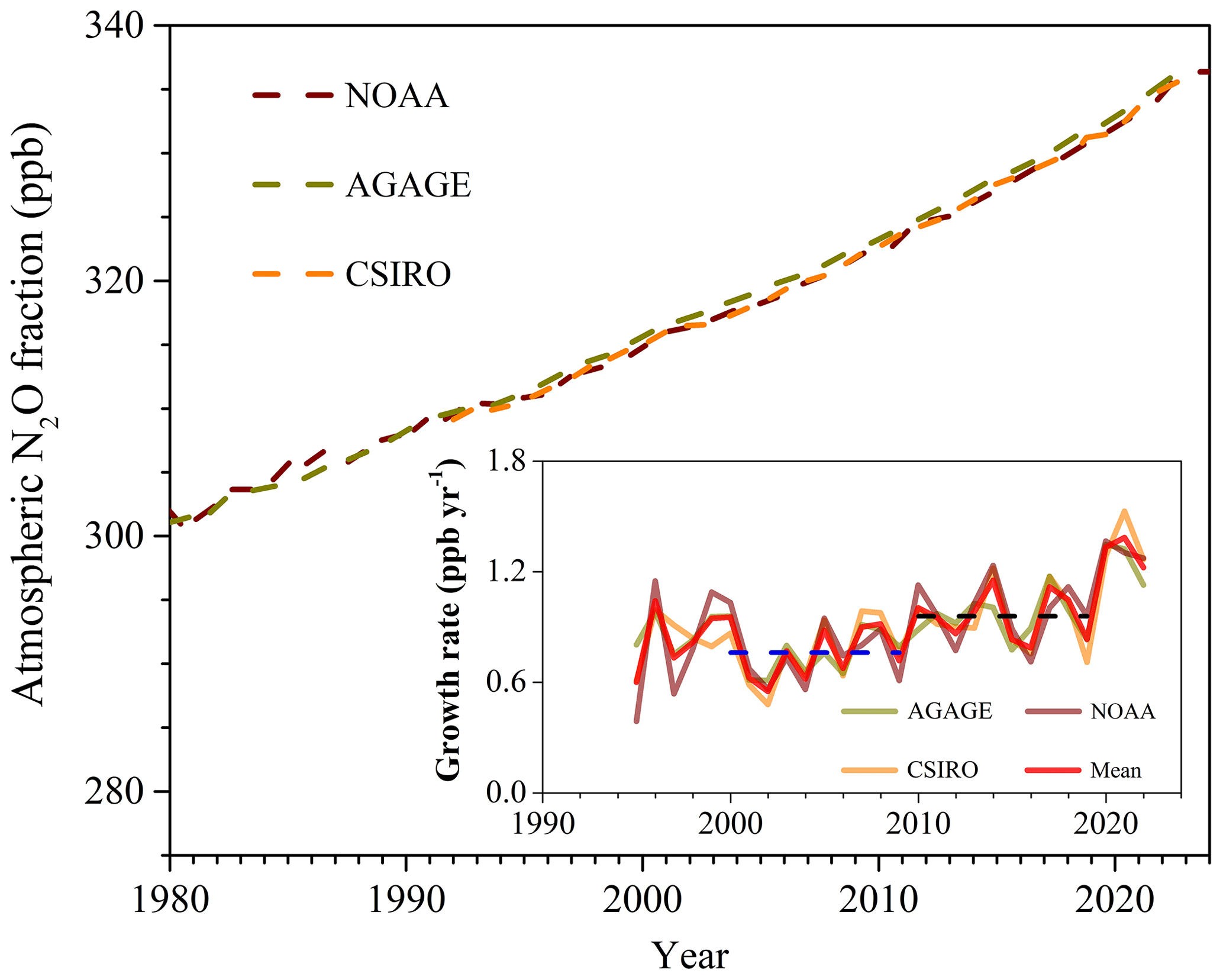
Figure 2Global mean atmospheric N2O dry mole fraction (atmospheric concentration) (1980–2022) and its annual growth rate (1995–2022) estimated by the AGAGE, NOAA, and CSIRO observing networks. The blue and black dashed lines represent the mean annual growth rate in the 2000s and 2010s, respectively.
Due to the rapid increase in global N2O emissions, observed atmospheric N2O mole fractions in recent years have begun to exceed the predicted levels under all scenarios in the Coupled Model Intercomparison Project Phase 6 (CMIP6) for the Sixth Assessment Report of the Intergovernmental Panel on Climate Change (IPCC, 2021; Gidden et al., 2019; Tian et al., 2020). N2O emissions are expected to continue increasing in the coming decades due to the growing demand for food, feed, fiber, and energy as well as a rising source from waste generation and industrial processes (Davidson and Kanter, 2014; Reay et al., 2012). Reducing N2O emissions will contribute to the mitigation of global warming and the recovery of stratospheric ozone (Jackson et al., 2019). It is noted that, although increased stratospheric NOx due to rising levels of N2O can lead to incremental stratospheric O3 loss, it is unlikely to cause catastrophic ozone loss the way that anthropogenic halogens did, as stratospheric NOx from N2O has offset halogen-catalyzed stratospheric ozone loss through various buffering reactions, e.g., the formation of halogen reservoir species like ClONO2 (Wennberg et al., 1994; Nevison et al., 1999; Ravishankara et al., 2009). Significant reductions in N2O emissions are required along with net CO2 emissions to stabilize the global climate system. For pathways consistent with the remaining carbon budget of 1.5, 1.7, and 2 °C stabilization, and assuming that all greenhouse gases (GHGs) should be cut in equal proportion to their contribution to anthropogenic radiative forcing, global N2O emissions need to be reduced by 22 %, 18 %, and 11 %, respectively, by 2050 (Rogelj and Lamboll, 2024). In addition, N2O mitigation could reduce ozone loss comparable to the depletion potential of the global chlorofluorocarbons (CFCs) stock in old air conditioners, refrigerators, insulation foams, and other units (UNEP, 2013). All in all, implementing N2O mitigation will contribute to achieving a set of United Nations Sustainable Development Goals (United Nations, 2016).
Nitrification and denitrification are the two key microbial processes controlling N2O production (Butterbach-Bahl et al., 2013; Gruber and Galloway, 2008; Kuypers et al., 2018; Firestone and Davidson, 1989), making the largest contribution to global N2O emissions (Syakila and Kroeze, 2011; Tian et al., 2020); abiotic processes also play a role in the production of N2O. We categorize the processes governing N2O sources and sinks in 23 different categories (Fig. 3): (1) Ffossil fuel – N2O emissions from fossil fuel combustion; (2) Findustry – N2O emissions from the chemical industry; (3) Fwaste water – N2O emissions from wastewater treatment and discharge; (4) Fnatural inland waters – natural N2O emissions from inland waters (rivers, lakes, and reservoirs); (5) Fhuman inland waters – anthropogenic N2O from inland waters (rivers, lakes, and reservoirs); (6) Fdirect soil emission – direct N2O emissions from agricultural soils; (7) Fmanure left on pasture – N2O emissions from manure left on pasture; (8) Fmanure management – N2O emission from manure management; (9) Faquaculture – N2O emissions from coastal and freshwater aquaculture; (10) – N2O emission/reduction due to land-cover change/deforestation; (11) Fnatural soil emissions – natural soil N2O emission; (12) Fbiomass burning – N2O emissions from biomass burning; (13) Fsurface uptake – surface N2O uptake; (14) FN deposition land – indirect N2O emissions from anthropogenic nitrogen additions on land; (15) FClimate effect – perturbed N2O fluxes from climate change; (16) – perturbed N2O fluxes from CO2 change; (17) Fshelves – N2O emission from continental shelves; (18) Foceans – N2O emission from open ocean; (19) FN deposition ocean – N2O emissions from anthropogenic N deposition on oceans; (20) Flightning and atmospheric production – lightning and atmospheric production of N2O; (21) Fstratospheric sink – stratospheric N2O sink; (22) Fnatural coastal water – natural N2O emissions from estuaries and coastal vegetation; and (23) FN dep and leaching – N2O emissions from nitrogen deposition and leaching to estuaries and coastal vegetation. There is also a small amount of N2O emission from termite mounds, but such an N2O flux is not quantified in the current budget analysis due to limited data.
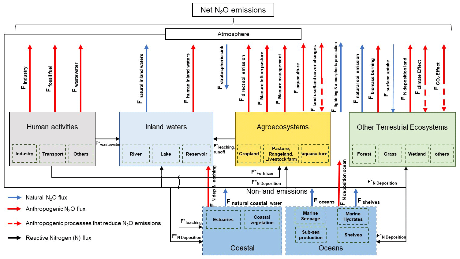
Figure 3N2O sources and sinks and flux partitions contributing to the global N2O budget. Upward-pointing arrows indicate a source to the atmosphere, whereas downward-pointing arrows represent a sink.
Biogenic N2O emissions from land are regulated by multiple environmental factors, including soil moisture, temperature, oxygen status, pH, vegetation type, topography, atmospheric CO2 concentration, and soil N and C availability (Butterbach-Bahl et al., 2013; Dijkstra et al., 2012; Li et al., 2020; Tian et al., 2016, 2019; Yin et al., 2022; H. Yu et al., 2022). The effects of these environmental factors on N2O emissions have strong spatial and temporal heterogeneity, making upscaling field N2O measurements to regional and global scales difficult. Studies using atmospheric N2O inverse modeling suggest a greater source of N2O from land and ocean under the colder and wetter La Nina conditions and vice versa in the warmer and drier El Niño conditions (Patra et al., 2022; Thompson et al., 2014). Ongoing environmental changes, such as ocean warming (and associated changes in stratification and ice coverage), decreasing pH (i.e., increasing acidification), loss of dissolved oxygen (i.e., deoxygenation), and eutrophication due to increasing anthropogenic inputs of nutrients via rivers and atmospheric deposition of nitrogen aerosols, might significantly alter the production and consumption of N2O in the upper ocean, its distribution pattern, and, ultimately, its release to the atmosphere (Bange et al., 2019; Bange, 2022; Wilson et al., 2020), exerting a small but uncertain feedback on global warming in the long term (Battaglia and Joos, 2018; Forster et al., 2021).
In this study, we construct a comprehensive global and regional N2O budget based on the processes and framework shown in Fig. 3 and following the framework of Tian et al. (2020). The figure summarizes the pathways of N2O formation, consumption, emission, and absorption, and it helps to guide consistent estimations and comparisons of N2O budgets among regions and upscaling of regional budgets to the globe. N2O fluxes are grouped into two major categories based on the sources.
The first category is natural N2O fluxes (blue arrows in Fig. 3), which are N2O fluxes in the absence of climate change and anthropogenic disturbances, including natural soil emissions, soil uptake, N2O emission from natural disturbances causing wetland loss and degradation, lightning, and atmospheric production. This category also includes natural emissions from inland waters, coastal ecosystems, and the ocean.
The second category is anthropogenic N2O fluxes (red arrows in Fig. 3). The direct emissions from nitrogen additions in the agricultural sector (“Agroecosystems” box in Fig. 3) include emissions from the direct application of synthetic nitrogen fertilizers and manure (henceforth “Direct soil emissions”), manure left on pasture, manure management, and aquaculture, while other direct anthropogenic sources include fossil fuel combustion and industry, waste and wastewater, and biomass burning. Indirect N2O emissions derive from anthropogenic nitrogen additions, such as atmospheric nitrogen deposition (NDEP) on land and ocean, and the effects of anthropogenic loads of reactive nitrogen in inland waters, estuaries, and coastal vegetation.
In the anthropogenic N2O fluxes category, we also consider N2O fluxes from the anthropogenic perturbations to climate, CO2, and land use/land cover (hereafter perturbation fluxes). In terrestrial ecosystems, perturbation fluxes can be caused by increasing CO2 concentration, climate change (e.g., warming-induced thawing of permafrost), and land-use change (e.g., converting natural lands to lands for human uses, such as croplands, mining, logging, and the post-deforestation pulse effect – the long-term effect of reduced mature forest area). N2O emissions can either increase or decrease during land conversion, depending on the type and phase of the land-use change. For example, when tropical forests are first converted to agriculture, there is often a pulse of N2O emissions for the first year or for as long as 5 years, depending upon the circumstances; following deforestation, emissions decline below those of the original forest if pastures degrade and if croplands are not fertilized, such as in slash-and-burn agriculture (Davidson and Artaxo, 2004; Meurer et al., 2016). When agriculture is abandoned and a secondary forest is allowed to regrow, N2O emissions gradually increase but usually remain lower than those of the original mature forest or from fertilized croplands (Davidson et al., 2007; Sullivan et al., 2019).
Numerous efforts have estimated individual sources and sinks of N2O across global ecosystems. Prominently, anthropogenic N2O emissions have been annually reported for the past 2 decades by Annex I Parties (developed countries) to the United Nations Framework Convention on Climate Change (UNFCCC) (https://unfccc.int/reports, last access: 1 November 2020). As a result of the Paris Agreement, over 190 signatory countries are now required to report their national GHG inventory biannually, if not already reported annually, with sufficient detail and transparency to track progress towards their nationally determined contributions. However, national GHG inventories only provide a partial picture of the observed changes in atmospheric N2O. They do not cover natural sources and have large uncertainties in the emission factors and activity data. Additionally, data are limited in many regions of the world, e.g., South America and Africa (Tian et al., 2020).
Tian et al. (2020) built the first comprehensive global N2O budget using multiple BU and TD methods as part of a partnership between the Global Carbon Project (GCP) and the International Nitrogen Initiative (INI). Based on Tian et al. (2020) and the budget framework established in Fig. 3, our study presents an improved and updated global N2O budget and its regional attribution to 18 land regions and the global ocean. The budgets cover the decades of 1980–1989, 1990–1999, 2000–2009, and 2010–2019 and includes a complete budget extension to 2020 and atmospheric N2O changes in 2021 and 2022. The work allows us to explore the relative temporal and spatial importance of multiple sources and sinks that drive the atmospheric burden of N2O, their uncertainties, and interactions between anthropogenic and natural forcings. This study also consolidates the international scientific capacity and networks that contribute to this assessment with the aim of providing improved and updated N2O budgets at regular intervals.
This global effort builds from and contributes to the set of global GHG assessments that the GCP has established, including regular updates of the carbon (CO2-C), methane (CH4), and (now) N2O budgets as well as other biogeochemical budgets of global significance. The budgets have been designed to (a) support global and national scientific assessments (e.g., IPCC and WCRP annual reports), (b) align scientific research and data products to support climate mitigation and sustainability policy needs, and (c) contribute to the Global Stocktake of the Paris Agreement to track progress towards nationally determined contributions and the ultimate goal of achieving net-zero GHG emissions. Integration of all GHGs in robust and shared methodological approaches and data delivery platforms are central goals of the GCP.
3.1 Definitions, terminology, and the unit of N2O sources and sinks
This study provides an estimation of the global N2O budget considering all quantifiable sources, sinks, and perturbations, resulting in a total of 21 N2O fluxes. To simplify our analysis, we further grouped these fluxes into six major categories: (1) “Natural baseline fluxes”, which is the source in the absence of climate change and anthropogenic disturbances and includes emissions from soils, surface uptake, shelf and ocean emissions, lightning and atmospheric production, and emissions from inland waters, estuaries, and coastal vegetation; (2) direct emissions from nitrogen additions in the agricultural sector (“Agriculture”), which includes emissions from the direct application of nitrogen fertilizers and manure (henceforth direct soil emissions), manure left on pasture, manure management, and aquaculture; (3) “Perturbed fluxes from climate, CO2, and land-cover change”, which includes the effects of CO2, climate, the post-deforestation pulse, and the long-term effect of reduced mature forest area; (4) indirect emissions from anthropogenic nitrogen additions, which includes atmospheric nitrogen deposition (NDEP) on the land, atmospheric NDEP on the ocean, and the effects of anthropogenic loads of reactive nitrogen in inland waters, estuaries, and coastal vegetation; (5) other direct anthropogenic sources, which includes fossil fuel and industry, waste and wastewater, and biomass burning; and (6) the atmospheric sink in the stratosphere (via photolysis and oxidation by O1D). Our anthropogenic N2O emission categories are aligned with those compiled by the national GHG inventories using IPCC (2006) methodologies and reported to the UNFCCC (Table A1).
In this study, N2O fluxes are expressed in teragrams of N2O-N per year, where 1 Tg N2O-N yr−1 (1 Tg N yr−1) = 1012 g N2O-N yr g N2O yr−1, with change rates in N2O fluxes expressed in teragrams of nitrous oxide-nitrogen per year squared (Tg N yr−2), representing the first derivative of annual N2O fluxes calculated by the linear regression method. Atmospheric N2O is expressed as dry air mole fractions, in parts per billion (ppb), with atmospheric N2O annual increases expressed in parts per billion per year (ppb yr−1). The conversion factor from the unit “ppb yr−1” to the unit “Tg N yr−1” is 4.79 Tg N ppb−1 (Prather et al., 2012). Unless specified, uncertainties are reported in parentheses as minimum and maximum values of all estimates, following Tian et al. (2020).
We focus on N2O fluxes and their change rates during three periods: 1997–2020, 1980–2020, and 2010–2019. For the time span from 1980 to 2020, which is the entire study period, we report temporal variations in BU estimates of N2O emissions from different sources to depict the overall trends of these fluxes. For the time span from 1997 to 2020, which is the overlapping period of BU and TD approaches, we compare BU and TD estimates to exam their consistency. For the time span from 2010 to 2019, which is the most recent decade, we report the magnitudes of emissions from different sources to give best estimates of their latest status and relative importance.
3.2 Definition of regions
As anthropogenic emissions are often reported at the country level, we divide global land into 18 regions and define these regions based on a country list (Table A2). This approach is compatible with all TD and BU approaches considered here. The number of regions was close to the widely used TransCom intercomparison map (Gurney et al., 2004) but with subdivisions to separate the contribution of important countries or regions to the global N2O budget (such as China, South Asia, and the USA). This regionalization is also compatible with the REgional Carbon Cycle Assessment and Processes (Poulter et al., 2022) after aggregation into 10 regions. The 18 regions are the United States (USA), Canada (CAN), Central America (CAM), northern South America (NSA), Brazil (BRA), southwestern South America (SSA), Europe (EU), northern Africa (NAF), equatorial Africa (EQAF), southern Africa (SAF), Russia (RUS), Central Asia (CAS), the Middle East (MIDE), China (CHN), Korea and Japan (KAJ), South Asia (SAS), Southeast Asia (SEAS), and Australasia (AUS). The region definition is the same as that used for the GCP methane and N2O budgets (Saunois et al., 2020; Stavert et al., 2022; Tian et al., 2019).
3.3 Overview of methods used for global N2O budget synthesis
Four major methods are available to estimate large-scale N2O emissions: atmospheric inversion models (method 1), activity- and emission-factor-based inventories (method 2), empirically based algorithms and machine learning algorithms (method 3), and process-based ecosystem models (method 4). Atmospheric inversion models (method 1), a TD approach, utilize measurements of atmospheric N2O mixing ratios combined with atmospheric transport models, driven by meteorological fields, to estimate the emissions of N2O (Thompson et al., 2014). Atmospheric inversion models usually use Bayesian statistics, which, starting from a prior emission estimate, find the optimal N2O emissions (i.e., those that best agree with observed atmospheric N2O mixing ratios) while also being guided by the prior emission and observation uncertainties (Nevison et al., 2018; Thompson et al., 2019).
TD approaches generally only estimate the total N2O emission, which is spatially and temporally resolved, but do not constrain the contributions from different sources. The other three methods belong to BU approaches, which are capable of quantifying N2O emissions from different sources. Emission-activity- and emission-factor-based inventories (method 2) use a prescribed emission factor (EF) to calculate N2O emissions. This approach has been widely used in national emission inventories and global studies (Davidson, 2009; Oreggioni et al., 2021; Crippa et al., 2021; Winiwarter et al., 2018). Nevertheless, the fixed EFs cannot capture the nonlinear response of agricultural soil N2O emissions to N inputs (Gerber et al., 2016) and also cannot fully reflect the dependence of EFs on climate, management practices, and soil physical and biochemical conditions (e.g., Marzadri et al., 2022). Therefore, a spatially referenced nonlinear model (SRNM), which outperformed the default EF method, was developed to simulate N2O emissions in response to fertilizer application under various environmental and management conditions (Zhou et al., 2015). In recent years, machine learning algorithms (method 3) have been applied to estimate soil N2O emissions. A random forest model was used to estimate global terrestrial background N2O emissions (Yin et al., 2022) and N2O emissions from intensively managed cropping systems (Saha et al., 2021). Moreover, a machine-learning-based stochastic gradient boosting model was developed to predict global terrestrial nitrification and its fraction in N2O emissions (Pan et al., 2021).
Compared with the three abovementioned methods, process-based ecosystem models (method 4) have two notable advantages (Xu et al., 2020; Tian et al., 2019): (1) they are capable of modeling the key processes affecting N2O production and emission, such as autotrophic nitrification, denitrification, plant nitrogen uptake, ammonia volatilization, nitrate leaching, and soil thermal and hydrological processes, although their accuracy in representing these processes needs further improvement; and (2) they integrate various driving factors controlling soil N2O emissions, such as fertilizer use, atmospheric N deposition, land-use change, climate change, and atmospheric CO2 concentration change and, thus, can disentangle the effects of different driving factors. Although multiple process-based models have estimated global soil N2O emissions, large discrepancies exist in these estimates due to the diverse parameterizations of biogeochemical processes in different models, our limited understanding of the mechanisms responsible for N2O emissions, and the uncertainties in input data. The Global N2O Model Intercomparison Project (NMIP) was launched (Tian et al., 2018, 2019) to develop a multi-model ensemble estimation of global soil N2O emissions during 1861–2016 and quantify the contributions of different driving factors.

Figure 4Methodologies used to estimate each of the main flux categories contributing to the global N2O budget. We use both BU and TD approaches, including 20 BU and 4 TD estimates of N2O fluxes from land and oceans. For sources estimated by the BU approach, we include eight process-based terrestrial biosphere modeling studies; six process-based ocean biogeochemical models and one shelf observational product; one nutrient budget model; five inland and coastal water modeling or meta-analysis studies; one statistical model SRNM based on spatial extrapolation of field measurements; and four greenhouse gas inventories – EDGAR v7.0, FAOSTAT, UNFCCC, and GFED. Previous estimates of the surface sink, lightning and atmospheric production, model-based tropospheric sink, and observed stratospheric sink are included in the current synthesis. The nutrient budget model provides nitrogen flows in global freshwater and marine aquaculture over the 1980–2020 period. Model-based estimates of N2O emissions from inland and coastal waters include rivers and reservoirs, lakes, estuaries, coastal vegetation (i.e., seagrasses, mangroves, and salt marsh), and coastal upwelling.
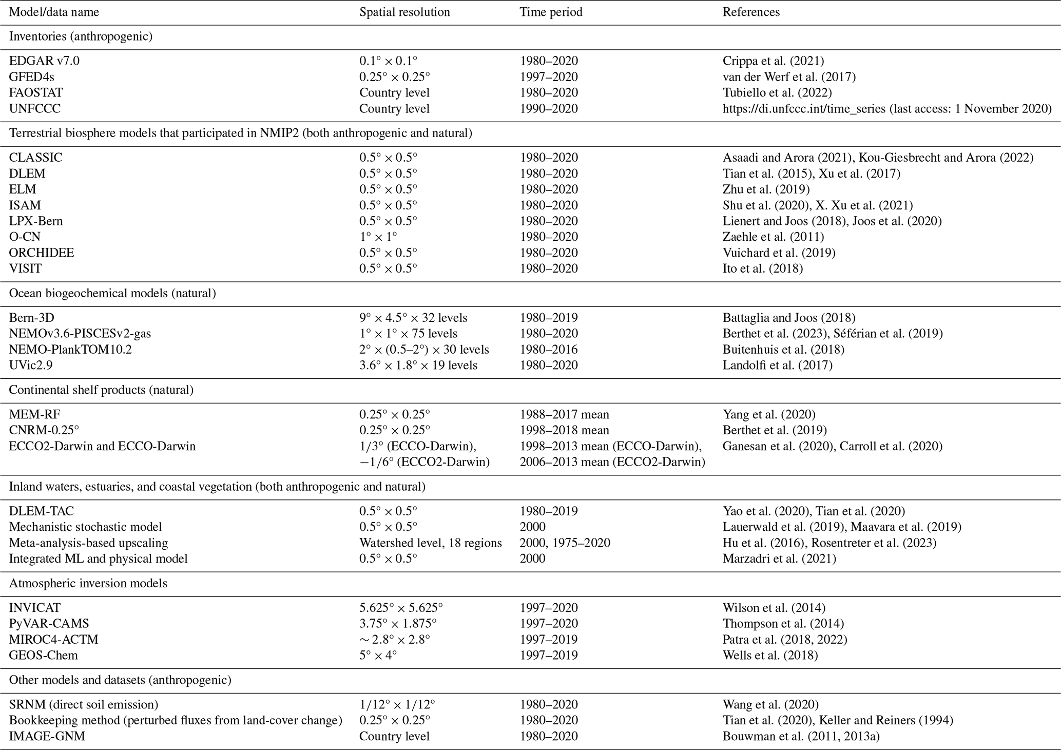
We consider global N2O emissions from land and ocean including natural fluxes and anthropogenic emissions based on BU and TD approaches (Fig. 4). The BU methods considered include eight process-based terrestrial biosphere models from NMIP2 (global Nitrogen/N2O Model Intercomparison Project phase 2); six ocean models (Battaglia and Joos, 2018; Berthet et al., 2023; Buitenhuis et al., 2018; Carroll et al., 2020; Landolfi et al., 2017); one machine-learning-based observational shelf product (Yang et al., 2020); a mix of five approaches relying on meta-analysis and statistical and process-based models for inland waters and coastal ecosystems (Hu et al., 2016; Lauerwald et al., 2019; Maavara et al., 2019; Yao et al., 2020; Marzadri et al., 2021; Marzadri et al., 2022; Rosentreter et al., 2023); four GHG emission databases – Emissions Database for Global Atmospheric Research (EDGAR) v7.0 (Crippa et al., 2021, https://edgar.jrc.ec.europa.eu/dataset_ghg70, last access: 10 February 2022), FAOSTAT (Tubiello et al., 2015), UNFCCC (https://unfccc.int/reports, last access: 1 November 2020), and GFED4s (van der Werf et al., 2017) (only for biomass burning); and one statistical model (SRNM) only for cropland soils (Wang et al., 2020). The TD approach consisted of four independent atmospheric inversion frameworks, namely INVICAT (Wilson et al., 2014), PyVAR-CAMS (Thompson et al., 2014), MIROC4-ACTM (Patra et al., 2022), and GEOS-Chem (Wells et al., 2018).
3.4 Model and inventory data synthesis
3.4.1 Natural N2O fluxes
“Natural soil baseline” emissions were obtained from the ensemble mean of the eight terrestrial biosphere models that participated in NMIP-2 that run with preindustrial land cover (Table 1): (1) the Canadian Land Surface Scheme including Biogeochemical Cycles (CLASSIC) (Asaadi and Arora, 2021; Melton et al., 2020; Kou-Giesbrecht and Arora, 2022); (2) the Dynamic Land Ecosystem Model (DLEM) (Tian et al., 2015; Xu et al., 2017; You et al., 2022); (3) the E3SM Land Model (ELM) (Zhu et al., 2019); (4) the Integrated Science Assessment Model (ISAM) (Shu et al., 2020; X. Xu et al., 2021); (5) the Land Processes and eXchanges model – Bern (LPX-Bern v1.4) (Lienert and Joos, 2018; Joos et al., 2020); (6) O-CN (Zaehle et al., 2011); (7) Organising Carbon and Hydrology In Dynamic Ecosystems (ORCHIDEE) (Goll et al., 2017); and (8) the Vegetation Integrated SImulator for Trace gases (VISIT) (Ito et al., 2018).
Table 1Methods, spatial and temporal resolution, and data sources for the synthesis of the global N2O budget.
Natural emission from “Inland water, estuaries, and coastal vegetation”, including inland and coastal waters, were obtained from models by Yao et al. (2020), Maavara et al. (2019), Lauerwald et al. (2019), and Marzadri et al. (2021) as well as the meta-analyses by Hu et al. (2016) and Rosentreter et al. (2023). As the data (rivers, lakes, reservoirs, and estuaries) provided by Hu et al. (2016), Maavara et al. (2019), Lauerwald et al. (2019), and Marzadri et al. (2021) are for the year 2000, we assumed that these values are constant during 1980–2020. Yao et al. (2020) provided annual riverine N2O emissions using DLEM during 1980–2019. Here, we averaged riverine estimates from Yao et al. (2020), Maavara et al. (2019), Hu et al. (2016), and Marzadri et al. (2021), assuming that the estimates of Maavara et al. (2019) and Hu et al. (2016) represent emissions from larger rivers only, while Yao et al. (2020) and Marzadri et al. (2021) also account for emissions from streams and small rivers. Note further that the estimate by Marzadri et al. (2021) is not fully global, as it excludes river systems north of 60° N. Therefore, we did not use this assessment for the regions of Canada, the USA, Russia, and Europe. DLEM also estimated annual N2O emissions from global reservoirs, and we averaged these estimates with those from Maavara et al. (2019) to represent emissions from reservoirs during 1980–2020. The estimate for global and regional lakes was based on the long-term average values provided by Lauerwald et al. (2019) and an estimate by the DLEM-TAC model (Li et al., 2024). For estuaries, we combined the estimate of Maavara et al. (2019), which relies on a process-based modeling approach, with a new meta-data analysis by Rosentreter et al. (2023). The analysis of Rosentreter et al. (2023) is observation-based and includes the contribution of coastal vegetated ecosystems, a contribution not accounted for in Maavara et al. (2019). Estuaries and coastal vegetation data are from studies published between 1975 and 2020, and we assume fluxes are constant during 1980–2020 (Rosentreter et al., 2023). To disentangle natural and anthropogenic fluxes, we considered the emissions in the year 1900 simulated by DLEM (Yao et al., 2020) as equivalent to the natural emission, assuming that the N load from land was negligible in that period (Kroeze et al., 1999). Using this approach, we estimated that N2O emissions from natural sources of rivers, reservoirs, lakes, and estuaries accounted for 44 % (36 %–52 %) of the total emissions from inland waters, taking into account all N inputs (i.e., inorganic, organic, dissolved, and particulate forms).
N2O emissions from continental shelves were calculated using one data-driven estimate and three high-resolution model estimates for various time periods (Resplandy et al., 2024, also see Sect. S7), namely an observation-based estimate that relied on a random forest (RF) algorithm to interpolate N2O data (Yang et al., 2020), based on a synthesis of over 158 000 observations of the N2O mixing ratio, partial pressure, and concentration in the surface ocean from the MEMENTO database (MEM-RF) (Kock and Bange, 2015); an estimate relying on the high-resolution configuration (Berthet et al., 2019) of the global ocean–biogeochemical component of CNRM-ESM2-1 (CNRM-0.25°); and two estimates relying on the ECCO-Darwin model run at ° (ECCO-Darwin1) and ° (ECCO-Darwin2), respectively. Considering that ECCO-Darwin1 and ECCO-Darwin2 relied on the same model, their mean N2O fluxes were used.
Estimates of natural N2O emissions from open oceans are derived from four global ocean biogeochemistry models, including Bern-3D (Battaglia and Joos, 2018), NEMOv3.6-PISCESv2-gas (Berthet et al., 2023), NEMO-PlankTOM10 (Buitenhuis et al., 2018), and UVic2.9 (Landolfi et al., 2017). Towards the N2O budget synthesis, modeling groups reported gridded monthly fluxes at a 1°×1° resolution for the 1980–2020 period. Specific details on ocean model configurations and N2O parameterizations are reported in the individual model publications.
We combined the estimate from lightning with that from atmospheric production into an integrated category “Lightning and atmospheric production” (Kohlmann and Poppe, 1999; Dentener and Crutzen, 1994). We simplified the Lightning and atmospheric production category as purely natural, although atmospheric production is affected to some extent by anthropogenic activities, such as enhancement of the concentrations of the reactive species NH3 and NO2. This category is, in any case, very small, and the anthropogenic enhancement effect is uncertain. The estimate of “Surface sink” was obtained from Schlesinger (2013) and Syakila et al. (2010).
3.4.2 Direct emissions from nitrogen additions (agriculture)
Agriculture N2O emissions consist of four components: “Direct soil emissions”, “Manure left on pasture”, “Manure management”, and “Aquaculture”. Data for direct soil emissions were obtained as the ensemble mean of N2O emissions from the average of two inventories (EDGAR v7.0 and FAOSTAT), the SRNM and DLEM models, and the NMIP2 and DLEM models. The statistical model SRNM only covers cropland N2O emissions. Thus, we added the DLEM-based estimate of pasture N2O emissions into the two estimates of cropland to represent direct agricultural soil emissions (i.e., SRNM/DLEM or NMIP2/DLEM). Manure left on pasture is the ensemble mean of EDGAR v7.0, FAOSTAT, and DLEM. Manure management emissions are the mean of EDGAR v7.0 and FAOSTAT. FAOSTAT emission factors for N additions are based on the 2006 guidelines. Global N flows (i.e., fish feed intake, fish harvest, and waste) in freshwater and marine aquaculture were obtained from Bouwman et al. (2011, 2013a) and Beusen et al. (2016) and based on the IMAGE-GNM aquaculture nutrient budget model for the 1980–2020 period. We then calculated global aquaculture N2O emissions as a 1.8 % loss of N waste in aquaculture, i.e., the same EF used in Hu et al. (2012) and MacLeod et al. (2019). The uncertainty range of the EF is from 0.5 % (Eggleston et al., 2006) to 5 % (Williams and Crutzen, 2010), the same range used in the UNEP report (Bouwman et al., 2013b).
3.4.3 Emissions from other direct anthropogenic sources
This category includes “Fossil fuel and industry”, “Waste and wastewater”, and “Biomass burning”. Both emissions from fossil fuel and industry and waste and wastewater were calculated as the ensemble means of EDGAR v7.0 and UNFCCC databases. The biomass burning emission is the ensemble mean of FAOSTAT, DLEM, and GFED4s databases. In EDGAR v7.0, the Waste and wastewater category includes “Waste incineration” and “Wastewater handling”. We merged “Transportation”, “Energy”, “Industry”, and “Residential and other sectors” to represent the total emission from fossil fuel and industry. The FAOSTAT emissions database of the Food and Agriculture Organization of the United Nations (FAO) covers emissions of N2O from agriculture and land use by country and globally, from 1961 to 2020 for agriculture and from 1990 for relevant land-use categories, i.e., cultivation of Histosols, biomass burning, etc., applying only Tier-1 coefficients (Tubiello et al., 2021, 2022; Conchedda and Tubiello, 2020; Prosperi et al., 2020). In addition to the IPCC agriculture burning categories “Burning crop residues” and “Burning savannah”, we included FAOSTAT estimates for N2O emissions from deforestation fires, forest fires, and peatland fires (Prosperi et al., 2020).
3.4.4 Indirect emissions from anthropogenic N additions
This category considers N deposition on land and the ocean (“N deposition on land” and “N deposition on ocean”) as well as the N leaching and runoff from upstream (“Inland and coastal waters”). The emission from N deposition on ocean was provided by Suntharalingam et al. (2012) and includes emission from both open oceans and continental shelves, while emission from N deposition on land was the average of two estimates by NMIP2/EDGAR v7.0 and NMIP2. EDGAR v7.0 provided estimates of indirect emissions from both agricultural and non-agricultural sectors; however, here, we sum the ensemble mean of NMIP2 estimates of indirect emissions from agricultural sectors with indirect emissions from the non-agricultural sector of EDGAR v7.0 (i.e., NMIP2/EDGAR v7.0) to represent N-deposition-induced soil emissions from both agricultural and non-agricultural sectors. The N2O emissions from inland and coastal waters consist of rivers, reservoirs, lakes, estuaries, and continental shelves, which is the ensemble mean of an average of two inventories (EDGAR v7.0 indirect N2O emissions – leaching and runoff – and FAOSTAT), and the mean of meta-analysis and models. The anthropogenic emission from inland freshwaters estimated by Yao et al. (2020) considered annual N inputs and other environmental factors (i.e., climate, elevated CO2, and land-cover change). The results in Yao et al. (2020) suggested that 56 % of the total N2O emissions from rivers, reservoirs, estuaries, and lakes was attributed to anthropogenic N additions. Empirical methods (empirical models and meta-analysis) adopted this ratio to calculate long-term average anthropogenic N2O emissions from inland waters, consistent with Tian et al. (2020). Seagrass, mangrove, and salt marsh N2O emissions were updated from Rosentreter et al. (2023).
3.4.5 Perturbation of N2O fluxes from climate, CO2, and land-cover change
The estimate of climate and CO2 effects on emissions was based on eight NMIP2 models, and we used SH1–SH7 and SH1–SH8 to model the effects of CO2 and climate on global terrestrial soil N2O emissions (Table 2), respectively. The effect of land-cover change on N2O dynamics includes the reduction due to the “Long-term effect of reduced mature forest area” and the additional emissions due to the “Post-deforestation pulse effect”. The two estimates were based on the bookkeeping approach and the DLEM model simulation. The bookkeeping method has been developed by Houghton et al. (1983) to account for carbon flows due to land use. In the original bookkeeping model developed by Houghton et al. (1983), land conversion and the affected carbon pools are tracked each year. The initial values of carbon pools are set for each type of land use. Annual changes in carbon pools in areas affected by land-use change or some land management practices (like wood harvest and fire management) are prescribed in the model using response curves, which are usually a function of the age of the newly converted land use. These response curves are specific for each type of land-cover type and land-use change and do not include the effects of environmental changes (Houghton and Castanho, 2023). For each age cohort, it either gains carbon (afforestation or reforestation) or loses carbon (deforestation) until its carbon pools reach a new stable state (the response curve converges). A similar bookkeeping method was developed to account for N2O emission due to deforestation. Here, different from the original bookkeeping model calculating carbon fluxes through tracking changes in vegetation or soil pools, response curves directly tracking annual N2O emissions after deforestation, which are also a function of the age of newly converted land use, were developed in our bookkeeping method (for details, please refer to Sect. S9).
Table 2Simulation design of NMIP2.
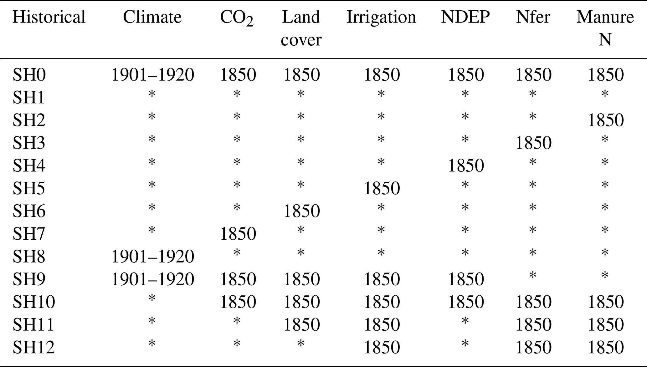
Note: for historical simulations, “*” indicates that the forcing during 1850–2020 is included in the simulation, “1901–1920” indicates that the 20-year mean climate condition during 1901–1920 will be used over the entire simulation period, and “1850” indicates that the forcing will be fixed in 1850 over the entire period. Climate data are only available from 1901; we assume the 20-year average value between 1901 and 1920 for the years 1850–1900. N deposition (NDEP) is available only from 1850. N fertilizer (Nfer) before 1910 was zero. Manure N is available only from 1860; we assume manure N at the 1860 value for the years 1850–1860.
3.4.6 Atmospheric production of reactive nitrogen
N2O production in the atmosphere is a relatively small component of the global budget. N2O is produced by the gaseous-phase oxidation of NH3 in the troposphere; however, there are few published estimates of this source, and it remains poorly constrained. In this paper, we refer to the two known published estimates, which are 0.4 Tg N yr−1 (Kohlmann and Poppe, 1999) and 0.6 (0.3–1.1) Tg N yr−1 (Dentener and Crutzen, 1994), that are derived using global models of atmospheric chemistry and transport. As human activities have greatly affected the atmospheric abundance of NH3, a significant portion of this source may be considered anthropogenic. Lightning production of NOx indirectly leads to N2O emission through its oxidation and subsequent deposition on land and the ocean. A recent study estimated the global lightning production of NOx to be 9 Tg N yr−1 (Nault et al., 2017), which is larger than previous estimates of 5 (2–8) Tg N yr−1 (Schumann and Huntrieser, 2007). In this study, we assume an effective emission factor of 1 % (De Klein et al., 2006); using the median estimate of 5 Tg N yr−1 of NOx, we then estimate a global source of N2O of 0.05 (0.02–0.09) Tg N yr−1. There is also N2O production from N2 + O(1D), which amounts to about 2 % of the atmospheric source in the stratosphere (Estupiñán et al., 2005).
3.5 Atmospheric observation data synthesis
3.5.1 Atmospheric burden and trends from tropospheric observations
The monthly tropospheric N2O mole fraction and its growth rate are derived from three different atmospheric observational networks: the Advanced Global Atmospheric Gases Experiment (AGAGE; Prinn et al., 2018), the Commonwealth Scientific and Industrial Research Organization (CSIRO; Francey et al., 2003), and the National Ocean and Atmospheric Administration (NOAA; Dutton et al., 2023; Lan et al., 2022). Further information on the three networks' stations, instruments, calibration, and uncertainties as well as access to data are provided in Sect. S12 “Atmospheric N2O Observation Networks”.
The atmospheric burden and its rate of change during 1980–2020 were derived from mean maritime surface abundance (mole fraction) of N2O (Prather et al., 2023) with a conversion factor of 4.79 Tg N ppb−1 (Prather et al., 2012). Combining uncertainties in measuring the annual mean surface mole fraction, which are <1 ppb (Dlugokencky et al., 1994), with those of converting surface mole fractions to a global mean abundance, we estimate a ±1.4 % uncertainty in the absolute burden (Prather et al., 2012). The uncertainty in the conversion from parts per billion to teragrams does not affect the trend uncertainty. This uncertainty is estimated to be ±0.2 ppb or ±1 Tg N between any 2 years over any recent period, based on the combined NOAA and AGAGE record of surface N2O taken from Table 2.1 of the IPCC AR5 (Hartmann et al., 2013). Thus, the uncertainty in the burden change between 2 decades (e.g., 2000s to 2010s) is bounded by ±1 Tg N (<0.1 %).
3.5.2 Atmospheric loss rates and trends from stratospheric observations
The NASA Aura Microwave Limb Sounder (MLS) satellite instrument has provided consistent global measurements of stratospheric N2O, O3, and temperature (T) since August 2004. These have been used with simple stratospheric chemistry models to calculate the monthly mean stratospheric loss of N2O due to photolysis and oxidation by O(1D) (Prather et al., 2015, 2023; Minschwaner et al., 1998). Tropospheric chemical loss also occurs, although at a very low rate (<1 % of the total) and is, thus, not included in the calculations.
3.5.3 Atmospheric inversion estimates of N2O emissions and losses
For the TD constraints on both land and ocean N2O fluxes for the 1998–2020 period, we used estimates from four independent atmospheric inversion frameworks (INVICAT, PyVAR-CAMS, MIROC4-ACTM, and GEOS-Chem), all of which used a Bayesian inversion method (see the Supplement for details on the inversion frameworks).
The inversion frameworks INVICAT and PyVAR-CAMS used the transport models TOMCAT and LMDz5, respectively, which were both driven by ECMWF ERA5 meteorology, while MIROC4-ACTM used the transport model ACTM, which was driven by JRA-55 meteorology, and GEOS-Chem used the transport model of the same name, which was driven by MERRA-2 meteorology. All inversion frameworks assumed that the prior distribution of emissions followed a normal distribution, with the multivariate mean taken from different models and data products, with standard deviations detailed in the Supplement. Specifically, GEOS-Chem, INVICAT, and PyVAR-CAMS built prior flux distributions for natural soil emissions from the terrestrial biospheric model O-CN (Zaehle et al., 2011) and for biomass burning emissions from GFED-v4s (van der Werf et al., 2017). For anthropogenic emissions from agricultural and non-agricultural sectors (excluding biomass burning), estimates from EDGAR v5 were used to build the prior for the 2005–2020 period (as these estimates were only available up to 2015, the emissions for 2016–2020 were estimated based on those of the year 2015), and the estimates from EDGAR-v4.32 were used for the 1997–2004 period. On the other hand, MIROC4-ACTM used the estimate from the terrestrial biospheric model VISIT for natural soil emissions and EDGAR v4.2 estimates for all anthropogenic emissions.
The inversion frameworks used atmospheric observations from ground-based networks, specifically NOAA, AGAGE, and CSIRO (see the Supplement for details).
The atmospheric transport models also calculate the loss of N2O in the stratosphere by photolysis and oxidation by O(1D) radicals (Minschwaner et al., 1998). The TD mean posterior estimates for the 18 land regions were calculated by integrating the gridded fluxes at 1°×1° over each region (the fluxes were interpolated from the original model resolution to 1°×1°).
4.1 Trends in atmospheric mole fractions and implied emissions
4.1.1 Trends in atmospheric N2O mole fractions
The three observation networks AGAGE, NOAA, and CSIRO show consistent growth in atmospheric N2O mole fractions from 315.8 (315.5–316.2) ppb in 2000 to 335.9 (335.6–336.1) ppb in 2022. The mean annual growth rate increased from 0.76 (0.55–0.95) ppb yr−1 in the 2000s to 0.96 (0.79–1.15) ppb yr−1in 2010s with significant seasonal and interannual variation. In 2020 and 2021, the N2O atmospheric growth rate was 1.33 and 1.38 ppb yr−1, respectively, both higher than any previous observed year (since 1980), and it was more than 30 % higher than the average value in the decade of the 2010s (Fig. 2). As is shown in Fig. 5, the observed N2O mole fraction in 2020 (333.2, 332.7–333.5 ppb) has exceeded predicted levels across the four illustrative Representative Concentration Pathways (RCPs) (329.2–331.5 ppb) used in CMIP5 (Meinshausen et al., 2011) and the seven illustrative Socioeconomic Pathways (SSPs) (330.5–331.9 ppb) used in CMIP6 (Meinshausen et al., 2020).

Figure 5Comparison between the measured global N2O mole fractions from the three GHG observing networks and the projected mole fractions from (a) the four illustrative Representative Concentration Pathways (RCPs) in the IPCC Fifth Assessment Report and (b) the seven illustrative Socioeconomic Pathways (SSPs) used in CMIP6.
4.2 N2O sources and sinks: BU estimates
4.2.1 Anthropogenic sources
Global anthropogenic emissions during 1980–2020
Global total anthropogenic emissions increased in the last 4 decades, from 4.8 (3.1–7.3) Tg N yr−1 in 1980 to 6.7 (3.3–10.9) Tg N yr−1 in 2020 (Fig. 6). Among all anthropogenic sources, direct emissions from nitrogen additions in the agricultural sector made the largest contribution to the increase, which grew from 2.2 (1.6–2.8) Tg N yr−1 in 1980 to 3.9 (2.9–5.1) Tg N yr−1 in 2020. Indirect N2O emissions also steadily increased during the study period, from 0.9 (0.7–1.1) Tg N yr−1 in 1980 to 1.3 (0.9–1.6) Tg N yr−1 in 2020. In contrast, other direct anthropogenic emissions did not have a trend, and the total amount fluctuated around 2.1 Tg N yr−1. Perturbed fluxes from climate, CO2, and land-cover change led to a small increase in the N2O sink, from −0.4 (−0.9 to 1.0) Tg N yr−1 in 1980 to −0.6 (−2.2 to 1.8) Tg N yr−1 in 2020.

Figure 6Changes in global anthropogenic N2O emissions (a) and N2O emissions from different sectors (b–e) during 1980–2020. In each panel, the line represents the mean N2O emission of different estimates, and the shaded area shows minimum and maximum estimates.
Direct emissions from nitrogen additions in the agricultural sector (agriculture)
In the past 4 decades, N2O emissions from all four sources within the agricultural sector significantly increased (Fig. 7), with the largest contribution from direct soil emissions (from 1.1 Tg N yr−1 in 1980 to 2.1 Tg N yr−1 in 2020), followed by manure left on pasture (from 0.9 Tg N yr−1 in 1980 to 1.4 Tg N yr−1 in 2020), aquaculture (from 0.01 Tg N yr−1 in 1980 to 0.12 Tg N yr−1 in 2020), and manure management (from 0.24 Tg N yr−1 in 1980 to 0.26 Tg N yr−1 in 2020).

Figure 7Changes in global direct N2O emissions from fertilizer and manure applied on agricultural soils (a), manure left on pasture (b), manure management (c), and aquaculture (d) during 1980–2020.
Direct soil emissions accounted for the largest proportion of emissions from the agriculture sector. All four estimates show a steady increase in direct soil emissions since 1980 (Fig. 7a). Among them, NMIP2/DLEM exhibited the largest magnitude and the fastest increase rate, from 1.1 Tg N yr−1 in 1980 to 2.6 Tg N yr−1 in 2020. By contrast, SRNM/DLEM suggested the slowest increase rate, from 1.0 Tg N yr−1 in 1980 to 1.7 Tg N yr−1 in 2020. The estimates of the two inventories (FAOSTAT and EDGARv7.0) exhibited similar magnitudes and trends, especially after 1990. All three estimates suggested a significant increasing trend for N2O emissions from manure left on pasture over the 1980–2020 period. Although all methods showed an increasing trend, they had significant differences in magnitude and increase rate (Fig. 7b). FAOSTAT showed the largest magnitude and increase rate, from 1.2 Tg N yr−1 in 1980 to 1.9 Tg N yr−1 in 2020. However, DLEM showed a smaller magnitude and a slower increase rate, from 0.5 Tg N yr−1 in 1980 to 0.9 Tg N yr−1 in 2020. Although the two inventory estimates for emissions from manure management showed similar temporal variations, FAOSTAT has a larger magnitude than EDGARv7.0 (Fig. 7c). According to the IMAGE-GNM aquaculture nutrient budget model, N2O emissions from aquaculture increased more than 10-fold, from 0.01 Tg N yr−1 in 1980 to 0.12 Tg N yr−1 in 2020 (Fig. 7d).
Other direct anthropogenic sources
Fossil fuel and industry emissions accounted for the largest proportion of N2O emissions from other direct anthropogenic sources. Estimates from two approaches showed different trends during their overlapping period: EGDARv7.0 had an increasing trend from 0.9 Tg N yr−1 in 1990 to 1.1 Tg N yr−1 in 2020, while EDGAR/UNFCCC did not show a trend with 1.0 Tg N yr−1 in 1990 and 1.0 Tg N yr−1 in 2020 (Fig. 8a). These inventories, however, do not capture a strong increase in emissions from adipic acid production since 2010 (Davidson and Winiwarter, 2023). Both EDGARv7.0 and EDGAR/UNFCCC show a steady and significant increase in N2O emissions from waste and wastewater. Although EDGAR/UNFCCC shows a larger magnitude than EGDARv7.0, these two inventory estimates display similar growth rates (Fig. 8b). There are large uncertainties in the magnitude and temporal trend in N2O emissions from biomass burning (Fig. 8c). DLEM and GFED show a larger magnitude of emissions than FAOSTAT. Both DLEM and GFED have a decreasing trend over the overlapping period from 1997 to 2020, but FAOSTAT shows no significant trend during this period.
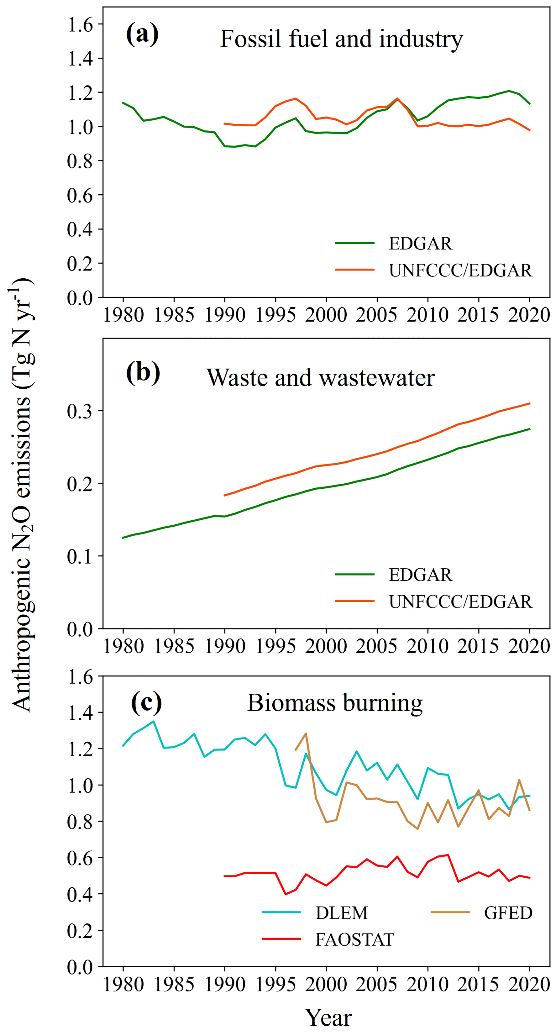
Figure 8Changes in N2O emissions from other direct anthropogenic sources between 1980 and 2020: fossil fuel (a), waste and wastewater (b), and biomass burning (c).
Indirect emissions from anthropogenic nitrogen additions
Global anthropogenic N2O emissions from inland waters, estuaries, and coastal vegetation continuously increased during 1980–2020 (Fig. 9a). Although all methods revealed an overall increasing trend in emissions, process-based models show a much smaller magnitude and increase rate than the two inventories. According to meta-analysis and models, anthropogenic emissions from inland and coastal waters increased from 0.1 Tg N yr−1 in 1980 to 0.15 Tg N yr−1 in 2020. In contrast, EGDARv7.0 and FAOSTAT showed that emissions increased from 0.33 and 0.35 Tg N yr−1 in 1980 to 0.53 and 0.57 Tg N yr−1 in 2020, respectively. Emissions from N deposition on land also continued to increase during 1980–2020 (Fig. 9b). NMIP2 and NMIP2/EDGAR v7.0 show emissions increasing from 0.6 and 0.4 Tg N yr−1 in 1980 to 0.9 and 0.6 Tg N yr−1 in 2020, respectively.
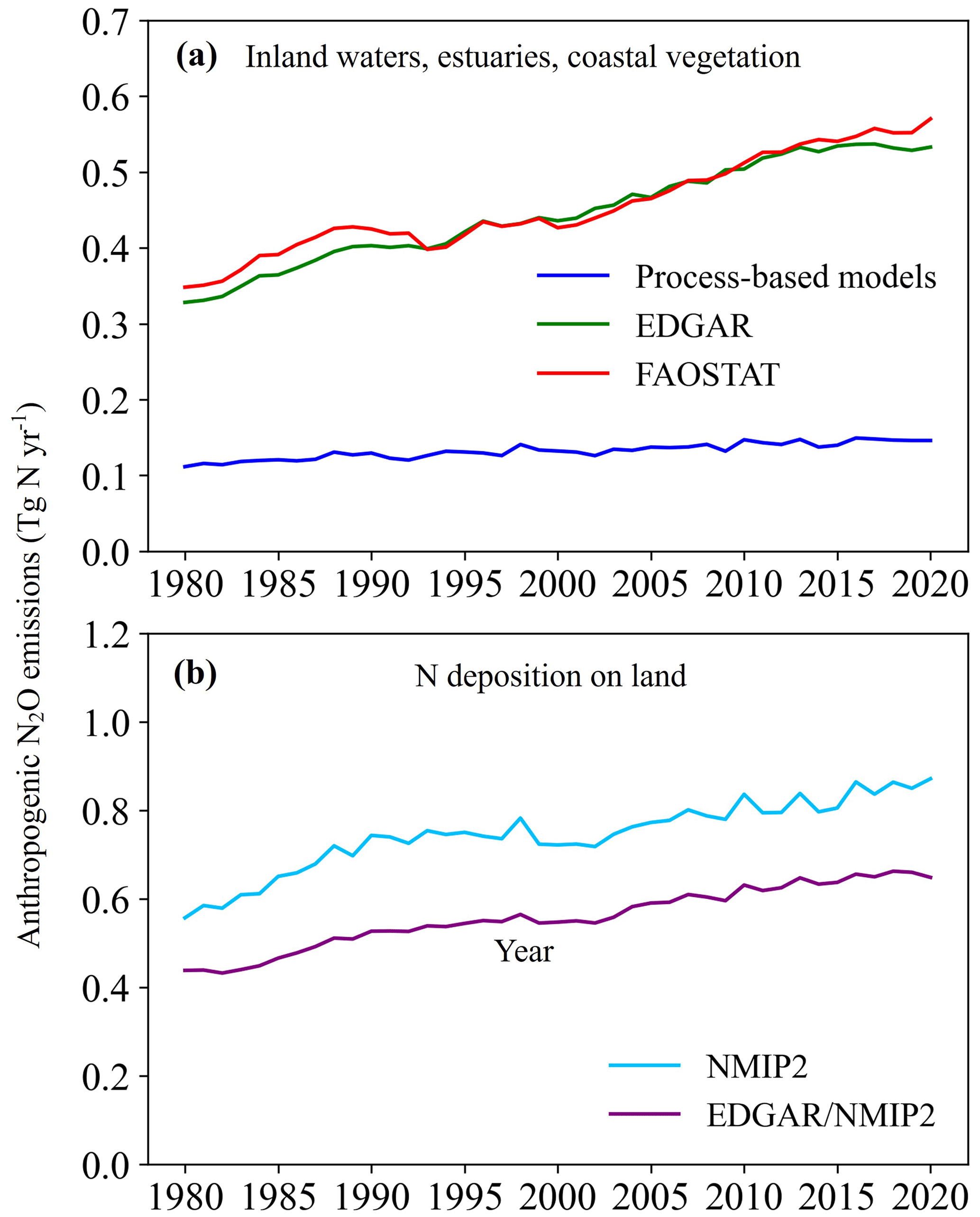
Figure 9Changes in indirect N2O emissions from anthropogenic nitrogen additions to inland waters (rivers, lakes, and reservoirs), estuaries, and coastal vegetation (a) as well as N deposition on land (b) during 1980–2020.
Perturbation fluxes from climate, CO2, and land-cover change
The spread between different estimates (DLEM and the bookkeeping method) of the post-deforestation pulse effect increased from the 1980s to the 2010s. The post-deforestation pulse effect was 0.8 (0.6–1.1) Tg N yr−1 in 1980 and 0.8 (0.4–1.3) Tg N yr−1 in 2020 (Fig. 10a). In contrast, DLEM and empirical approaches are comparable in terms of the magnitude and temporal changes in the long-term reduction effect of deforestation, with both approaches suggesting a strong long-term reduction effect, which grew from −1.2 (−1.0, −1.4) Tg N yr−1 in 1980 to −1.4 (−1.3, −1.6) Tg N yr−1 in 2020 (Fig. 10b). In general, deforestation had a negative effect on global soil N2O emissions. However, most NMIP2 models suggested a positive effect of climate change on soil N2O emissions, although with large uncertainty and significant interannual variation; this positive climate feedback significantly increased during the past 4 decades (Fig. 10c). In contrast to climatic effects, most NMIP2 models suggested a negative effect of rising atmospheric CO2 concentration on soil N2O emissions through increasing nitrogen use efficiency and, hence, reducing soil N availability (Fig. 10d). However, NMIP2 models have large discrepancies in the CO2 fertilization effect on N2O emissions; ELM and ISAM suggested a positive effect, while all the other models suggest a negative effect.
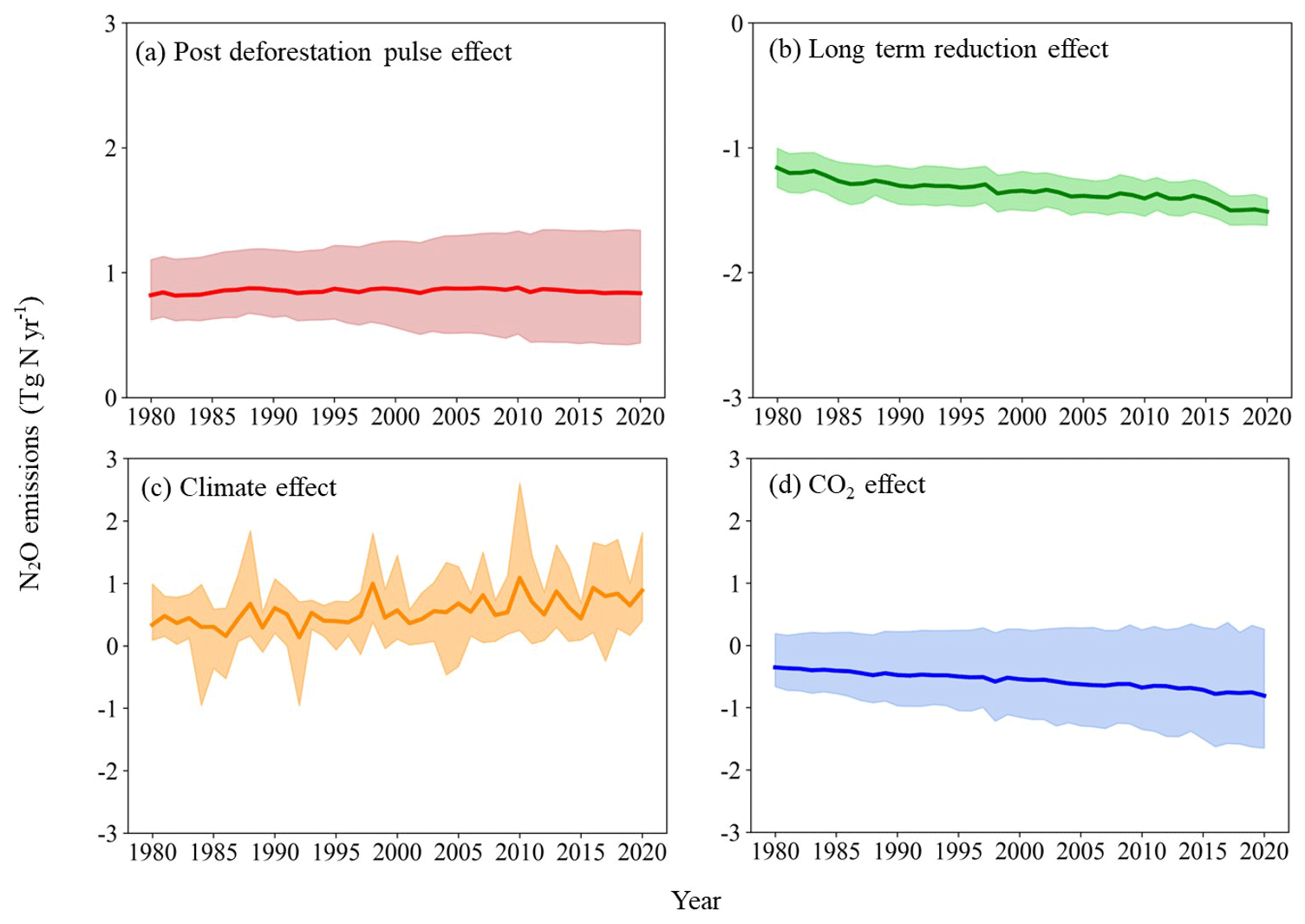
Figure 10Changes in perturbed N2O fluxes from changes in climate, CO2, and land cover during 1980–2020. In each panel, the line represents the mean N2O emission of different estimates, and the shaded area shows minimum and maximum estimates.
4.2.2 Natural N2O sources
Emissions from natural soils and open oceans remained relatively steady throughout the study period from 1980 to 2020, with mean estimates fluctuating between 9.9 and 10.3 Tg N yr−1 (minimum estimates: 6.2–7.1 Tg N yr−1; maximum estimates: 12.8–13.6 Tg N yr−1). Natural emissions from all other sources including shelves, inland waters, and lightning and atmospheric production were assumed to be constant during 1980–2020. According to BU approaches, the total natural emissions from these sources were 1.8 (1.0–3.0) Tg N yr−1. The mean value of global N2O emissions from all of the abovementioned sources fluctuated between 11.7 and 12.1 Tg N yr−1, with an average of 11.9 Tg N yr−1. Global natural N2O emissions also have a large uncertainty, with the maximum estimates (15.8–16.6 Tg N yr−1) roughly double the minimum estimates (7.1–8.1 Tg N yr−1).
Natural soil N2O emission baseline
The natural soil N2O emission baseline represents the preindustrial soil N2O emissions derived from NMIP2 simulations, driven by potential vegetation/land cover and other environmental factors in the preindustrial period (1850). Global natural soil N2O emissions are estimated to be 6.4 Tg N yr−1, and they account for 55 % of the total natural emissions. However, N2O emissions from natural soils estimated by the NMIP2 showed large divergences among eight models. Among the NMIP2 models, ELM had the highest estimate with an average of 8.6 Tg N yr−1, which was more than double the estimate from the CLASSIC model (3.9 Tg N yr−1).
Natural N2O emission baseline from the open ocean and continental shelves
We also estimated N2O emissions from the open oceans and continental shelves. Open ocean is the second largest source of natural N2O emissions, with a global mean value fluctuating between 3.4 and 3.8 Tg N yr−1 during 1980–2020. Open-ocean N2O emissions were estimated by four ocean models. Among these models, NEMOv3.6-PISCESv2-gas had the highest estimate, with an average of 4.6 Tg N yr−1, while NEMO-PlankTOM10 had the lowest estimate, with an average of 2.8 Tg N yr−1. The four ocean models show different trends in open-ocean emissions. NEMOv3.6-PISCESv2-gas shows a slight increasing trend, whereas the other three models show consistent decreasing trends. In addition to open oceans, shelves are an important source of N2O emissions that was not quantified in the previous global N2O budget (Tian et al., 2020). Global shelf N2O emissions were estimated by two high-resolution models (CNRM and ECCO) and one data product (MEM-RF). The average of the three estimates is 1.2 Tg N yr−1, ranging from 0.6 Tg N yr−1 (ECCO) to 1.6 Tg N yr−1 (MEM-RF).
Natural N2O emission from inland waters, estuaries, and coastal vegetation
Natural N2O emissions from inland waters and estuaries were much smaller than emissions from the soils, oceans, and shelves. These emissions have an average value of 0.08 Tg N yr−1, ranging from 0.05 to 0.14 Tg N yr−1. Rivers are the largest source: they emit 0.04 (0.01–0.08) Tg N yr−1 of N2O and account for 48 % of the natural emissions from inland waters and estuaries. The global natural N2O emissions from lakes and estuaries were 0.02 (0.01–0.03) and 0.02 (0.02–0.03) Tg N yr−1, respectively.
Lightning, atmospheric production, and natural sinks
The source of reactive N from lightning (and its contribution to N2O) and the direct production of N2O from NH3 in the atmosphere are relatively small, and we have no new estimates in this work. However, synthesizing the available estimates in the scientific literature, we estimate lightning to contribute 0.05 (0.02–0.09) Tg N yr−1 (median and range) (Nault et al., 2017; Schumann and Huntrieser, 2007) and atmospheric production to contribute 0.5 (0.3–1.1) Tg N yr−1 (Kohlmann and Poppe, 1999; Dentener and Crutzen, 1994).
Similarly, the surface sink of N2O is small. Again, we do not produce a new estimate in this budget and rather only synthesize available estimates from the literature. We estimate the global surface sink to be 0.01 (0.0–0.3) Tg N yr−1.

Figure 11Annual global N2O emissions during 1997–2020 estimated by four atmospheric inversions (TD models): (a) total global emission, (b) land emission, and (c) ocean emission.
4.3 N2O sources and sinks: TD estimates
4.3.1 TD total source
Ensemble estimates across the four atmospheric inversions show that the long-term average global N2O emissions during 1997–2020 were 16.6 Tg N yr−1 (minimum: 15.5 Tg N yr−1; maximum: 18.2 Tg N yr−1). All four inversions show a significant increasing trend in global N2O emissions (p<0.05) with a mean rate of increase of 0.10 Tg N yr−2 (0.08–0.12 Tg N yr−2) (Fig. 11a).
TD land emission
The estimates derived from the four inversions show that the land-based emission is the dominant source of N2O emissions, over ocean sources, and the long-term average land N2O emission during 1997–2020 was 13.7 Tg N yr−1 (minimum: 12.6 Tg N yr−1; maximum: 15.0 Tg N yr−1), contributing 80 %–85 % of the global N2O emissions. Land sources dominated the interannual variability in global N2O emissions and the trend (Fig. 11b). All TD models suggested a significant increasing trend in land N2O emissions during the study period from 1997 to 2020 (p<0.05), with increase rates ranging from 0.09 to 0.13 Tg N yr−2, which were higher than the increase rates of prior fluxes (mean: 0.04 Tg N yr−2; range: 0.00–0.08 Tg N yr−2).
TD ocean emission
The magnitude of N2O emissions from oceans is much smaller than that from land (Fig. 11c). The mean ocean N2O emission during 1997–2020 derived from four inversion models was 2.9 Tg N yr−1, ranging from a minimum of 2.7 Tg N yr−1 to a maximum of 3.3 Tg N yr−1. The estimates of MIROC4 were much higher than the estimates of other models. The four inversions show divergent interannual variability, and none suggested a significant trend. The TD estimates of ocean N2O emission are much smaller than the values estimated by four ocean biogeochemical models, with a global mean value fluctuating between 3.4 and 3.8 Tg N yr−1 during 1980–2020.
4.3.2 TD stratospheric sink
The four inversions have comparable magnitudes of global stratospheric N2O sink (via photolysis and oxidation by the electronically excited atomic oxygen, O(1D), in the stratosphere), with an average value of 12.4 Tg N yr−1 (minimum and maximum of 12.2 and 12.7 Tg N yr−1, respectively) for 2000–2020 (Fig. 12). All four inversions found that the global stratospheric N2O sink increased during 1997–2020 (Fig. 13) in proportion to the growing atmospheric N2O abundance, with an average rate of increase of 0.05 Tg N yr−2 (0.03–0.07 Tg N yr−2). Differences among the estimates decreased after 2000, likely due to improvements in observation coverage and accuracy but also possibly due to the decreasing influence of the initial mixing ratio fields, which differed among the inversion frameworks. Although the inversions show comparable trends in the sink, they differ with respect to their interannual variability.
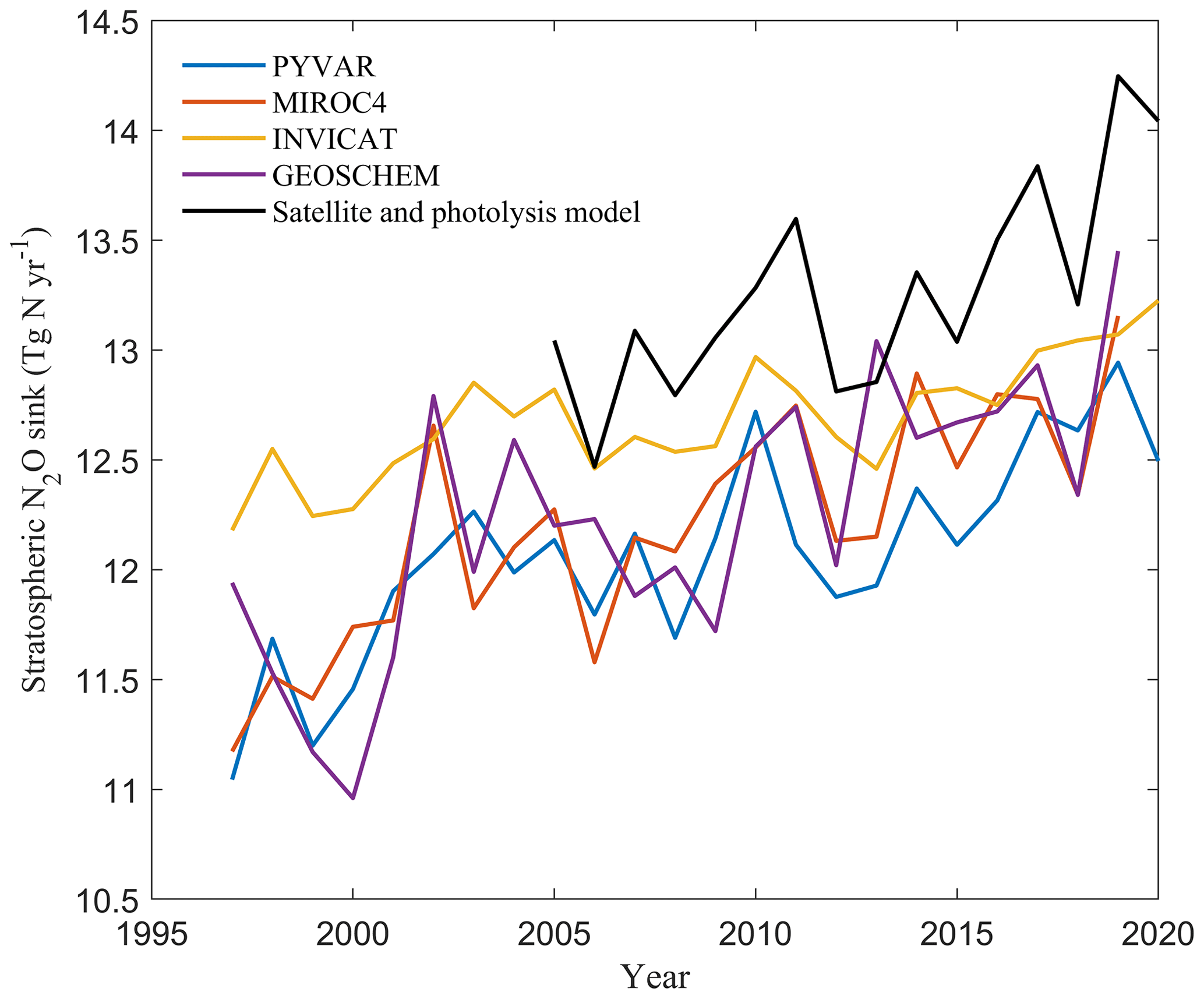
Figure 12Global stratospheric N2O sink estimated by atmospheric inversions and a satellite and photolysis model during 1997–2020.
Table 3The global N2O budget (in Tg N yr−1) for the 1980s, the 1990s, the 2000s, the 2010s, and the year 2020.
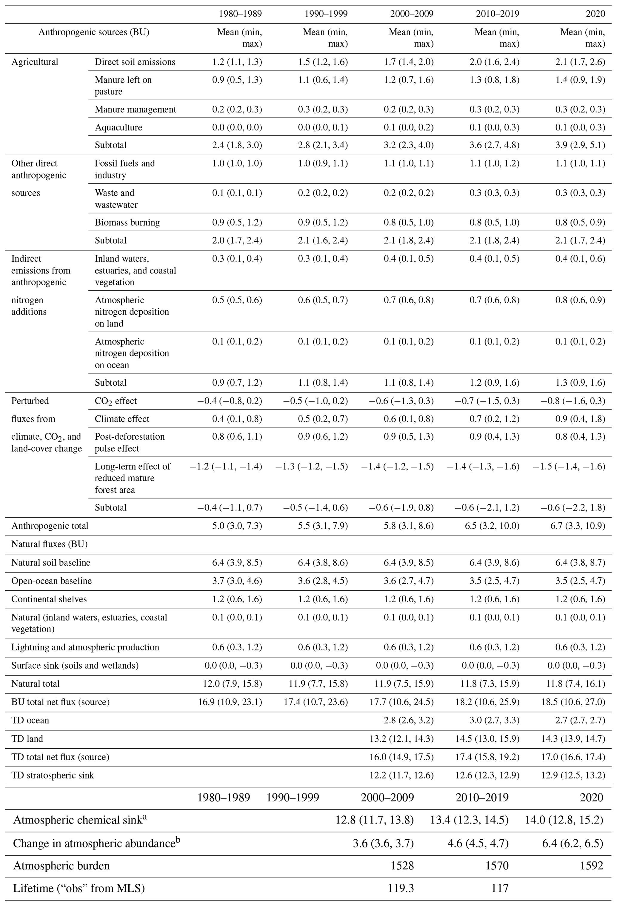
Notes: BU estimates include four categories of anthropogenic source and one category for natural sources and sinks. The sources and sinks of N2O are given in teragrams of nitrogen per year (Tg N yr−1). The atmospheric burden is given in teragrams of nitrogen (Tg N). Detailed information on calculating each subcategory is shown in tables in the Supplement. a Calculated from satellite observations with a photolysis model (about 1 % of this sink occurs in the troposphere). b Calculated from the combined NOAA and AGAGE record of surface N2O and adopting the uncertainty of the IPCC Fifth Assessment Report (Chap. 6), with a conversion factor of 4.79 Tg N ppb−1.
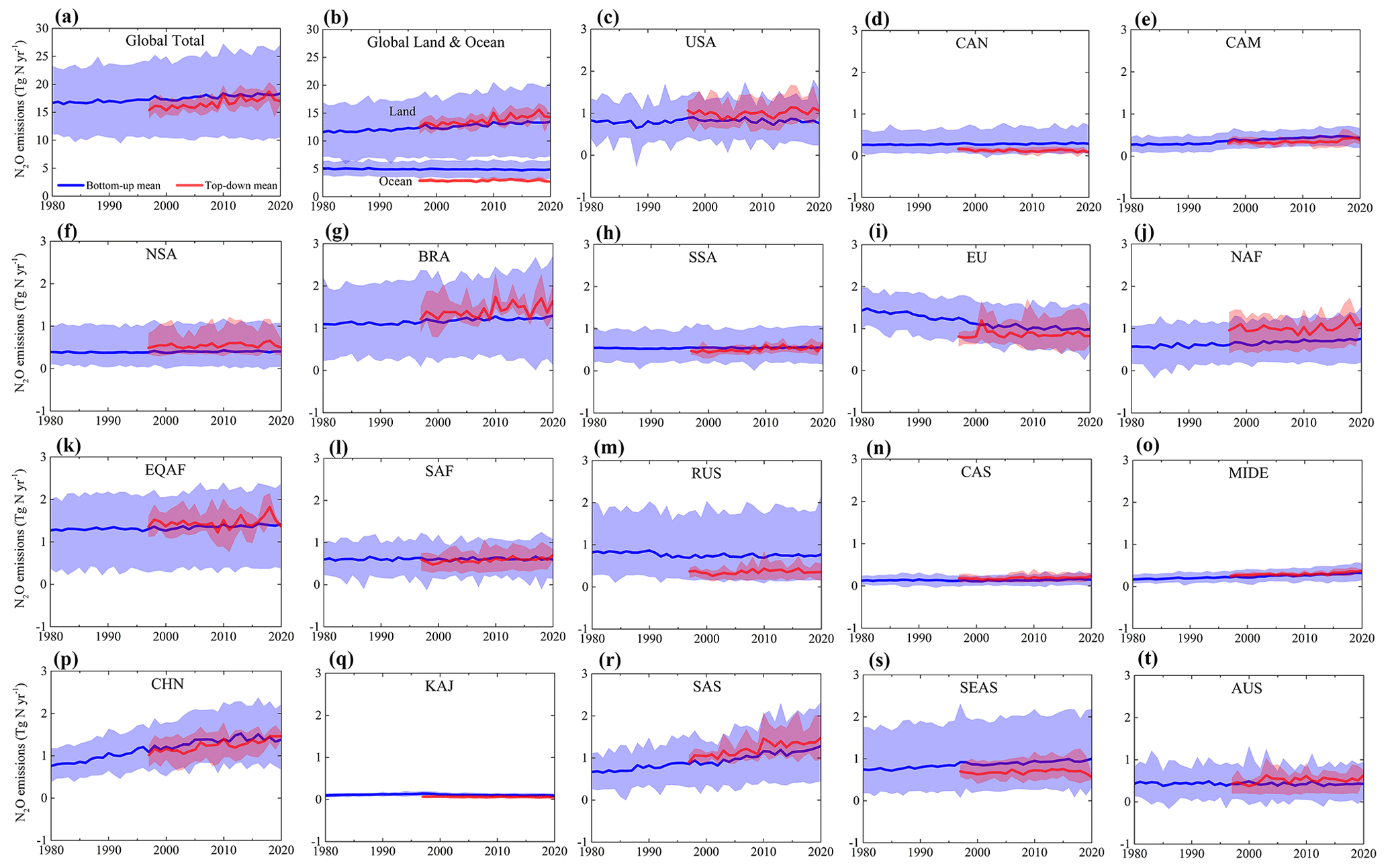
Figure 13Comparison of global and regional N2O emissions estimated using BU and TD approaches. The 18 regions include the United States (USA), Canada (CAN), Central America (CAM), northern South America (NSA), Brazil (BRA), southwestern South America (SSA), Europe (EU), northern Africa (NAF), equatorial Africa (EQAF), southern Africa (SAF), Russia (RUS), Central Asia (CAS), the Middle East (MIDE), China (CHN), Korea and Japan (KAJ), South Asia (SAS), Southeast Asia (SEAS), and Australasia (AUS). The blue lines represent the mean N2O emission from BU methods, and the shaded areas show minimum and maximum estimates; the red lines represent the mean N2O emission from TD methods, and the shaded areas show minimum and maximum estimates.
We also provide an independent estimate of the stratospheric sink based on satellite observations and a photolysis model. This estimate likewise showed that the sink increased, from 12.8 Tg N yr−1 in the 1990s to 14.0 Tg N yr−1 in the 2010s (Table 3), with higher annual loss rates than estimated by the inversions and an average loss of 13.4 Tg N yr−1 for 2005–2021. This estimate also showed large quasi-biennial interannual variability with an amplitude of 7 %. More interestingly, over this time period, the abundance of N2O in the middle stratosphere, where the greatest loss of N2O occurs, was increasing at a rate of 5.0±1.2 % per decade, which is faster than the increase in the tropospheric abundance of 2.9±0.0 % per decade. This resulted in a greater loss of N2O (i.e., more than proportionate to the mean atmospheric increase) and, thus, a decrease in the mean atmospheric lifetime (burden divided by loss) of 2.1±0.7 % per decade, from 119.3 years in the 2000s to 117 years in the 2010s (Prather et al., 2023; also see Table 3). These changes are thought to be a result of an increase in the intensity of the Brewer–Dobson circulation (BDC), which would transport N2O more rapidly from the troposphere into the mid-stratosphere. An increase in the intensity of BDC is predicted by climate models (Oberländer-Hayn et al., 2016). However, we note that none of the atmospheric inversions found a significant trend in the atmospheric lifetime (although the total loss increased; Fig. 12), and more research is needed to identify why there is this discrepancy.
4.4 Decadal patterns and trend in the global N2O budget: comparisons between BU and TD approaches
BU approaches provide estimates of N2O fluxes for the identified sources and sinks during 1980–2020, while TD approaches only provide the total net flux during 1997–2020. In the following analyses of the decadal global N2O budget, the comparison between BU and TD approaches is only for total N2O estimates. We rely on BU approaches to quantify all identified sources and sinks (Table 3, Fig. 1).
4.4.1 Global N2O budget in recent decade (2010–2019)
The BU and TD approaches give remarkably consistent estimates of global total N2O emissions in the 2010s, with values of 18.2 (10.6–25.9) Tg N yr−1 and 17.4 (15.8–19.2) Tg N yr−1 (Fig. 1, Table 3), respectively. However, the BU estimate shows a large uncertainty range, in part because of the spread of estimates from process-based models. TD approaches estimate that the stratospheric sink (i.e., N2O losses via photolysis and reaction with O(1D) in the stratosphere) for the 2010s was 12.6 (12.3–12.9) Tg N yr−1. However, the atmospheric sink estimate based on satellite observations and a photolysis model for the 2010s was 13.4 (12.3–14.5) Tg N yr−1. The imbalance of sources and sinks of N2O derived from the averaged BU and TD estimates is 4.7 Tg N yr−1. This imbalance agrees well with the observed increase in atmospheric abundance of N2O between 2010 and 2019 of 4.6 (4.5–4.7) Tg N yr−1. Based on the BU-based estimates, natural sources contributed 65 % of total emissions (11.8, 7.3–15.9 Tg N yr−1) during this period. Specifically, the natural soil flux contributed the most, with the decadal mean of 6.4 (3.9–8.6) Tg N yr−1, followed by the open-ocean emissions (3.5, 2.5–4.7 Tg N yr−1), shelf emissions (1.2, 0.6–1.6 Tg N yr−1), lightning and atmospheric production (0.6, 0.3–1.2 Tg N yr−1), and natural emissions from inland waters and estuaries (0.1, 0.0–0.1 Tg N yr−1) (Fig. 1).
Anthropogenic sources contributed, on average, 35 % to the total N2O emissions (6.5, 3.2–10.0 Tg N yr−1) in the 2010s. Direct emissions from nitrogen additions in agriculture were 3.6 (2.7–4.8) Tg N yr−1, contributing 56 % of the total anthropogenic emissions (Table 3). Emissions from other direct anthropogenic sources made the second largest contribution, with a decadal mean of 2.1 (1.8–2.4) Tg N yr−1. Indirect emissions from anthropogenic nitrogen additions contributed 19 % of the total anthropogenic emissions, with a decadal mean of 1.2 (0.9–1.6) Tg N yr−1. Changes in climate, CO2, and land cover had an overall negative effect on N2O emissions (−0.6, −2.1 to 1.2 Tg N yr−1), mainly because of the negative effects of reduced mature forest area (−1.4, −1.6 to −1.3 Tg N yr−1) and increasing CO2 concentration (−0.7, −1.5 to −0.3 Tg N yr−1).
4.4.2 Decadal trend in the global N2O budget
Global N2O emissions estimated by the BU and TD approaches were comparable in magnitude during the overlapping period from 1997 to 2020, but TD estimates implied a larger interannual variability and a faster rate of increase (Fig. 13a). BU and TD approaches diverge when estimating the magnitude of land emissions compared with ocean emissions, although they are consistent with respect to trends (Fig. 13b). According to the BU approaches, global N2O emissions increased from 17.4 Tg N yr−1 (10.3–24.0 Tg N yr−1) in 1997 to 18.5 Tg N yr−1 (10.6–27.0 Tg N yr−1) in 2020, with an average increase rate of 0.043 Tg N yr−2 (p<0.05). In contrast, TD approaches suggested that global emissions increased from 15.4 Tg N yr−1 (13.9–16.7 Tg N yr−1) in 1997 to 17.0 Tg N yr−1 (16.6–17.4 Tg N yr−1) in 2020, implying a higher increase rate of 0.085 Tg N yr−2 (p<0.05). The BU estimate during 1997–2010 was on average 1.6 Tg N yr−1 higher than the TD estimate. However, after 2010, the difference in the magnitude of emissions between the two approaches is smaller, due to the rapid increase in the TD estimates. From the year 1980, BU approaches suggested a significant increase in global N2O emissions that was primarily driven by anthropogenic sources (Table 3). Satellite and photolysis models estimate that the atmospheric N2O burden increased from 1528 Tg N in the 2000s to 1570 in the 2010s and 1592 Tg N in 2020, which is comparable to estimates by atmospheric chemistry transport models, showing an increase in the atmospheric N2O burden from 1527 (1504–1545) Tg N in the 2000s to 1606 (1592–1621) Tg N in 2020.

Figure 14Ensembles of regional anthropogenic N2O emissions over the 1980–2020 period. The bar chart in the center shows the total changes in regional and global N2O emissions during the study period from 1980 to 2020. Error bars indicate the 95 % confidence interval for the average of the changes. A Mann–Kendall test was performed to establish any trends globally and for each region over the 1980–2020 period. The changes were calculated from the annual change rate (Tg N yr−2), determined from a linear regression, multiplied by 40 years. All regions except Australasia and the USA show a significant increasing or decreasing trend in the estimated ensemble N2O emissions during 1980–2020. An asterisk (*) denotes significance at the P<0.05 level.
4.5 Regional BU and TD estimates and their trends
To assess regional N2O budgets, we divide the global land into 18 regions (as described in Sect. 3). Our regional analyses include the following: (1) trends and variations in regional total N2O emissions from all sources derived from available TD (1997–2020) and BU (1980–2020) estimates (Fig. 13), (2) trends and variations in region anthropogenic N2O emissions from all identified sources during 1980–2020 derived from a BU approach (Fig. 14), and (3) decadal regional N2O budget (2010–2019) derived from both BU and TD approaches (Fig. 15). The following sections provide detailed estimates for each of the 18 regions.
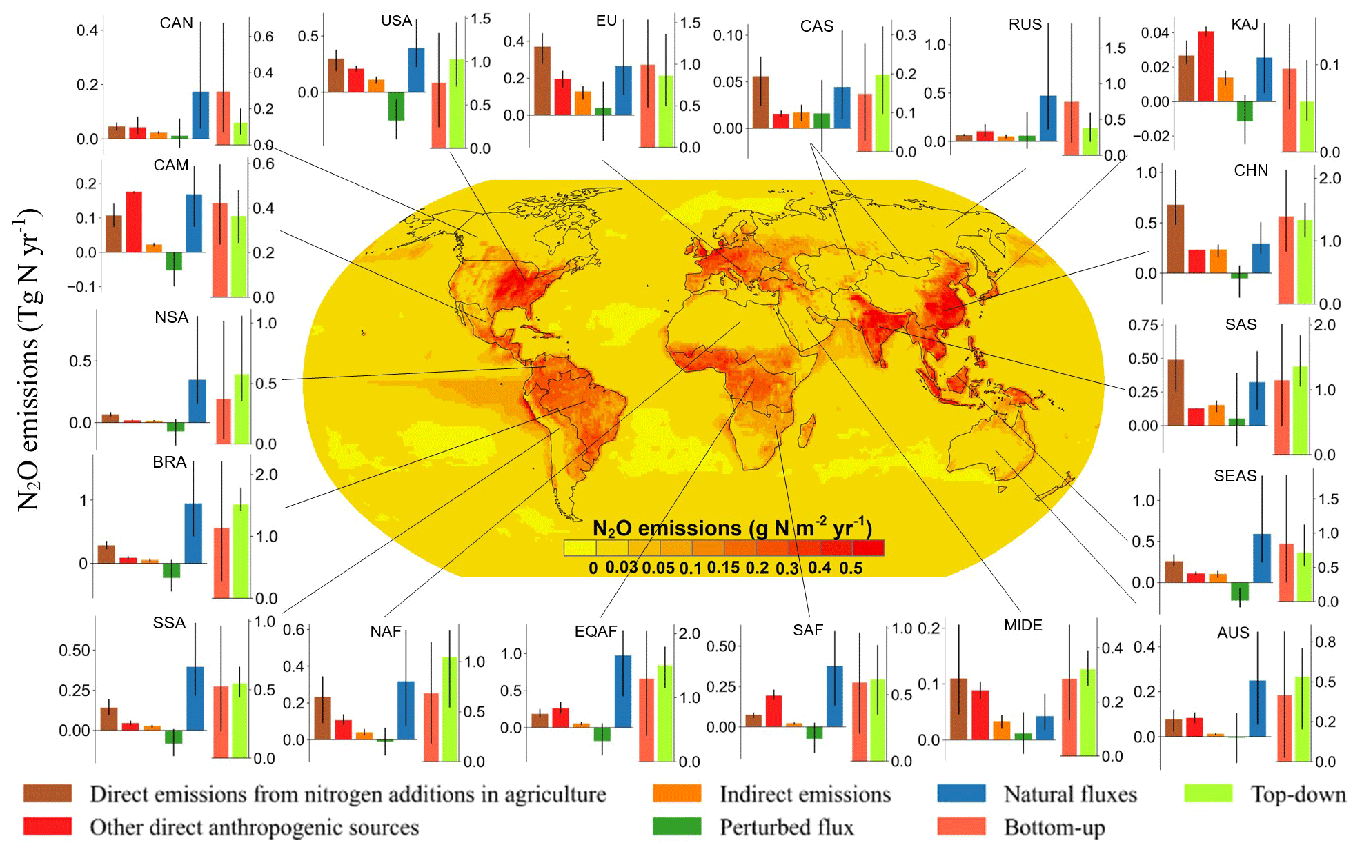
Figure 15Regional N2O emissions during 2010–2019. Each subplot shows the emissions from five subsectors using BU approaches, followed by the sum of these five categories using BU approaches (coral) and the estimates from TD approaches (lime). Error bars indicate the spread between the minimum and the maximum values. The center map shows the spatial distribution of 10-year average N2O emissions from land and the ocean based on the land and ocean models.
4.5.1 United States of America (USA)
For the USA, the TD estimates show higher total N2O emissions than the BU estimates over the 1997–2020 period (Fig. 13c), with 1.00 (0.69–1.39) and 0.82 (0.31–1.42) Tg N yr−1, respectively. Both approaches suggest that the total N2O emissions from the USA remained relatively stable during 1997–2020. Based on the BU estimates, changes in climate, CO2, and land cover caused emission decline over 1980–2020. The flux fluctuated between −0.30 and −0.12 Tg N yr−1, with an average of −0.20 Tg N yr−1. Indirect emissions from anthropogenic nitrogen additions increased from 0.11 Tg N yr−1 in 1980 to 0.13 Tg N yr−1 in 1995 and then decreased to 0.10 Tg N yr−1 in 2020. Direct emissions from nitrogen additions in agriculture increased from 0.25 Tg N yr−1 in 1980 to 0.30 Tg N yr−1 in 2020. However, the increase in direct agricultural emissions was offset by the trend in emissions from other direct anthropogenic sources, which decreased from 0.26 Tg N yr−1 in 1980 to 0.19 Tg N yr−1 in 2020. The total anthropogenic N2O emissions slightly increased during 1980–2020, at an average rate of Tg N yr−2. This increase primarily occurred during 1980–1997 (Fig. 14).
In the 2010s, the BU estimates (0.81, 0.29–1.43 Tg N yr−1) were on average 0.22 Tg N yr−1 lower than the TD estimates (1.03, 0.71–1.45 Tg N yr−1) (Fig. 15). According to the BU results, natural sources contributed 48 % of total emissions (0.39, 0.22–0.65 Tg N yr−1) during this period. Direct emissions from nitrogen additions in agriculture were 0.30 (0.18–0.38) Tg N yr−1, contributing 37 % of the total emissions. Emissions from other direct anthropogenic sources made the second largest contribution to anthropogenic emissions, with a decadal mean of 0.21 (0.18–0.23) Tg N yr−1. Indirect emissions from anthropogenic nitrogen additions contributed 14 % of the total anthropogenic emissions, with a decadal mean of 0.11 (0.07–0.14) Tg N yr−1. Changes in climate, CO2, and land cover had an overall negative effect on N2O emissions, with a mean value of −0.19 Tg N yr−1 and range of −0.37 to 0.03 Tg N yr−1. Recent study has indicated that N2O emissions could be increased by freeze–thaw cycles (Del Grosso et al., 2022) and tillage practices (Lu et al., 2022). Our BU estimates did not consider freeze–thaw cycles or tillage practices and, thus, may have underestimated N2O emissions.
4.5.2 Canada (CAN)
BU approaches suggested a larger magnitude of total N2O emissions from Canada than TD approaches over the 1997–2020 period (Fig. 13d), with values of 0.29 (0.05–0.69) and 0.12 (0.06–0.19) Tg N yr−1, respectively. BU and TD estimates also showed divergent trends: TD estimates decreased at a rate of Tg N yr−2, whereas BU estimates increased at a rate of Tg N yr−2. According to the BU results, the increase in total N2O emissions from Canada was mainly driven by the direct emissions from nitrogen additions in agriculture, which increased from 0.02 Tg N yr−1 in 1980 to 0.05 Tg N yr−1 in 2020. Perturbed fluxes from changes in climate, CO2, and land cover showed an overall increase from 0.00 Tg N yr−1 in 1980 to 0.02 Tg N yr−1 in 2020. Indirect N2O emissions from Canada were relatively stable during the study period, while emissions from other direct anthropogenic sources had large interannual variability (Fig. 14).
In the 2010s, the BU estimates of Canada's total N2O emissions (0.29, 0.07–0.69 Tg N yr−1) were over 2 times higher than the TD estimates (0.12, 0.06–0.20 Tg N yr−1) (Fig. 15). According to the BU results, natural sources contributed 59 % of total emissions (0.17, 0.04–0.43 Tg N yr−1) during this period. Direct emissions from nitrogen additions in agriculture were 0.05 (0.03–0.06) Tg N yr−1, contributing 15 % of the total emissions. Emissions from other direct anthropogenic sources and indirect emissions from anthropogenic nitrogen additions were 0.04 (0.02–0.08) and 0.02 (0.02–0.03) Tg N yr−1, respectively. Changes in climate, CO2, and land cover had an overall positive effect on N2O emissions, with a mean value of 0.01 Tg N yr−1 and a range of −0.04 to 0.09 Tg N yr−1.
4.5.3 Central America (CAM)
TD and BU estimates are comparable with respect to the magnitudes and trends of N2O emissions from Central America (Fig. 13e), with mean values of 0.42 (0.21–0.64) and 0.35 (0.25–0.47) Tg N yr−1 for the BU and TD approaches, respectively. During 1997–2020, the rate of increase of the BU estimates ( Tg N yr−2) was higher than that of TD estimates ( Tg N yr−2). Emissions from other direct anthropogenic sources increased from 0.03 Tg N yr−1 in 1980 to 0.15 Tg N yr−1 in 2020 and were the major driver of the increase in N2O emissions from Central America. Direct agricultural emissions increased during the study period, from 0.08 Tg N yr−1 in 1980 to 0.11 Tg N yr−1 in 2020. Indirect emissions and perturbed fluxes from changes in climate, CO2, and land cover were relatively stable during this period (Fig. 14).
The BU and TD approaches gave comparable estimates of total N2O emissions from Central America in the 2010s, with values of 0.46 (0.24–0.68) and 0.36 (0.24–0.48) Tg N yr−1 for the BU and TD approaches (Fig. 15), respectively. Natural sources contributed 37 % of total emissions (0.17, 0.07–0.26 Tg N yr−1) during this period. Emissions from other direct anthropogenic sources contributed 39 % of the total emissions (0.18, 0.17–0.18 Tg N yr−1). Direct and indirect emissions were 0.11 (0.07–0.14) and 0.02 (0.02–0.03) Tg N yr−1, respectively. Changes in climate, CO2, and land cover had an overall negative effect on N2O emissions, with a mean value of −0.02 Tg N yr−1 and a range of −0.10 to 0.07 Tg N yr−1.
4.5.4 Northern South America (NSA)
TD approaches suggested a larger magnitude of total N2O emissions from northern South America than BU approaches over the 1997–2020 period (Fig. 13f), with respective values of 0.55 (0.34–0.98) and 0.40 (0.04–1.08) Tg N yr−1 for each approach. During 1997–2020, the increase rate of the TD estimates ( Tg N yr−2) was higher than that of BU estimates ( Tg N yr−2). Direct agricultural emissions made the largest contribution to the increase in N2O emissions from northern South America, increasing from 0.04 Tg N yr−1 in 1980 to 0.07 Tg N yr−1 in 2020 (Fig. 14). N2O emissions from the other three anthropogenic sectors did not have a significant trend during 1980–2020.
The BU estimates in the 2010s (0.41, 0.03–1.09 Tg N yr−1) were on average 0.17 Tg N yr−1 lower than the TD estimates (0.58, 0.35–1.06 Tg N yr−1) (Fig. 15). The average natural emission was 0.35 Tg N yr−1 in the 2010s, contributing 85 % of total emissions. Direct agricultural emissions, other direct emissions, and indirect emissions were 0.07 (0.05–0.09), 0.02 (0.01–0.02), and 0.01 (0.01–0.02) Tg N yr−1, respectively. Changes in climate, CO2, and land cover had an overall negative effect on N2O emissions, with a mean value of −0.04 Tg N yr−1 and a range of −0.19 to 0.10 Tg N yr−1.
4.5.5 Brazil (BRA)
The average total N2O emission from Brazil estimated by the BU approaches was 1.21 Tg N yr−1, ranging from 0.26 to 2.32 Tg N yr−1 (Fig. 13g), which was lower than the TD estimates (1.42, 1.18–1.75 Tg N yr−1). Both approaches detected a notable increasing trend in total N2O emissions during 1997–2020. TD approaches suggested a higher increase rate ( Tg N yr−2) than BU approaches ( Tg N yr−2). Direct agricultural emissions, which increased from 0.13 Tg N yr−1 in 1980 to 0.32 Tg N yr−1 in 2020, made the largest contribution to the increase in N2O emissions from Brazil (Fig. 14). Indirect emissions also showed an increase from 0.03 Tg N yr−1 in 1980 to 0.06 Tg N yr−1 in 2020. Emissions from other anthropogenic sources and perturbed fluxes from changes in climate, CO2, and land cover did not have an obvious trend during the study period.
The TD estimates in the 2010s (1.51, 1.40–1.79 Tg N yr−1) were on average 0.28 Tg N yr−1 higher than the BU estimates (1.23, 0.24–2.41 Tg N yr−1) (Fig. 15). According to the BU results, the average natural emission was 0.95 Tg N yr−1 in the 2010s, contributing 77 % of total emissions. Direct agricultural emissions, other direct emissions, and indirect emissions were 0.28 (0.22–0.35), 0.09 (0.06–0.11), and 0.05 (0.02–0.07) Tg N yr−1, respectively. Changes in climate, CO2, and land cover had an overall negative effect on N2O emissions, with a mean value of −0.14 Tg N yr−1 and a range of −0.48 to 0.25 Tg N yr−1.
4.5.6 Southwest South America (SSA)
BU and TD estimates are consistent with respect to the magnitude of the total N2O emissions from southwestern South America during 1997–2020, with values of 0.55 (0.18–1.03) and 0.51 (0.40–0.63) Tg N yr−1 (Fig. 13h), respectively. TD estimates increased at a rate of Tg N yr−2 over 1997–2020, whereas BU estimates did not have an obvious trend during this period. Among the four anthropogenic sectors, direct agricultural emissions had the largest increase, from 0.10 Tg N yr−1 in 1980 to 0.15 Tg N yr−1 in 2020 (Fig. 14). Indirect emissions also increased from 0.02 Tg N yr−1 in 1980 to 0.03 Tg N yr−1 in 2020. Perturbed fluxes from changes in climate, CO2, and land cover had a decreasing trend, while emissions from other sectors fluctuated over the study period.
The BU and TD approaches gave similar estimates of total N2O emissions from southwestern South America in the 2010s, with values of 0.55 (0.19–1.04) and 0.55 (0.44–0.67) Tg N yr−1 (Fig. 15), respectively. The mean natural emission was 0.39 Tg N yr−1 in the 2010s, accounting for 71 % of total emissions. Direct agricultural emissions, other direct emissions, and indirect emissions were 0.14 (0.09–0.19), 0.05 (0.03–0.06), and 0.03 (0.01–0.03) Tg N yr−1, respectively. Changes in climate, CO2, and land cover had an overall negative effect on N2O emissions, with a mean value of −0.05 Tg N yr−1 and a range of −0.16 to 0.08 Tg N yr−1.
4.5.7 Europe (EU)
The BU estimates suggest that Europe had the largest decrease rate of regional N2O emissions among the 18 regions, and the average decrease rate during 1980–2020 was Tg N yr−2 (Fig. 13i). For the 1997–2020 period, this decreasing trend, as estimated by the BU approaches, slowed down ( Tg N yr−2), whereas the TD approach suggests a small increase of Tg N yr−2 (Fig. 13i). Emissions from other direct anthropogenic sources (including fossil fuel and industry, waste and wastewater, and biomass burning), which decreased from 0.51 Tg N yr−1 in 1980 to 0.18 Tg N yr−1 in 2020, made the largest contribution to the decreasing trend in N2O emissions from Europe. Direct agricultural emissions and indirect emissions show overall decreasing trends from 0.46 and 0.16 Tg N yr−1 in 1980 to 0.38 and 0.12 Tg N yr−1 in 2020, respectively, mainly due to a reduction in fertilizer use after the collapse of the Soviet Union (Tian et al., 2022). However, the decreasing trend in direct agricultural emissions has leveled off since the 2000s. Perturbed fluxes from changes in climate, CO2, and land cover decreased during 1980–1985 and then slowly increased (Fig. 14).
The BU and TD approaches gave comparable estimates of European N2O emissions in the 2010s, with values of 1.00 (0.45–1.57) and 0.86 (0.49–1.36) Tg N yr−1 (Fig. 15), respectively. According to the BU results, natural sources only contributed 26 % of total emissions (0.26, 0.11–0.52 Tg N yr−1) during this period. Direct agricultural emissions, other direct emissions, and indirect emissions were 0.38 (0.32–0.44), 0.19 (0.15–0.24), and 0.13 (0.08–0.16) Tg N yr−1, respectively. Changes in climate, CO2, and land cover had an overall positive effect on N2O emissions, with a mean value of 0.03 Tg N yr−1 and a range of −0.21 to 0.22 Tg N yr−1.
4.5.8 Northern Africa (NAF)
For northern Africa, TD approaches suggested a larger magnitude of the total N2O emissions than BU approaches over the 1997–2020 period (Fig. 13j), with values of 1.01 (0.52–1.32) and 0.69 (0.18–1.27) Tg N yr−1, respectively. Both approaches suggest that N2O emissions from northern Africa significantly increased during 1997–2020, and the increase rates estimated by the BU and TD approaches were and Tg N yr−2, respectively. Direct emissions increased from 0.10 Tg N yr−1 in 1980 to 0.27 Tg N yr−1 in 2020, making the largest contribution to the increase in N2O emissions from northern Africa (Fig. 14). Indirect emissions also significantly increased from 0.02 Tg N yr−1 in 1980 to 0.04 Tg N yr−1 in 2020. In contrast, other anthropogenic emissions decreased from 0.12 Tg N yr−1 in 1980 to 0.11 Tg N yr−1 in 2020. N2O fluxes caused by changes in climate, CO2, and land cover remained relatively stable during 1980–2020.
In the 2010s, the BU estimates (0.72, 0.17–1.30 Tg N yr−1) were on average 0.32 Tg N yr−1 lower than the TD estimates (1.04, 0.54–1.31 Tg N yr−1) (Fig. 15). Natural sources accounted for 44 % of total emissions (0.32, 0.07–0.60 Tg N yr−1) during this period. Direct emissions from nitrogen additions in agriculture were 0.23 (0.09–0.34) Tg N yr−1, contributing 32 % of the total emissions. Emissions from other direct anthropogenic sources made the second largest contribution to anthropogenic emissions, with a decadal mean of 0.11 (0.08–0.14) Tg N yr−1. Indirect emissions and perturbed fluxes from changes in climate, CO2, and land cover were 0.04 (0.02–0.06) Tg N yr−1, and 0.02 (−0.10 to 0.16), respectively.
4.5.9 Equatorial Africa (EQAF)
Similar to northern Africa, TD approaches suggested a larger magnitude of total N2O emissions from equatorial Africa than BU approaches over the 1997–2020 period (Fig. 13k), with values of 1.45 (1.15–1.78) and 1.36 (0.36–2.22) Tg N yr−1, respectively. Both approaches suggested that N2O emissions from equatorial Africa significantly increased during 1997–2020, and the increase rates estimated by the BU and TD approaches were and Tg N yr−1, respectively. Direct emissions more than tripled during the study period, from 0.07 Tg N yr−1 in 1980 to 0.22 Tg N yr−1 in 2020, dominating the increase in N2O emissions from equatorial Africa (Fig. 14). Indirect emissions also steadily increased from 0.04 Tg N yr−1 in 1980 to 0.06 Tg N yr−1 in 2020. On the contrary, perturbed fluxes from changes in climate, CO2, and land cover showed an overall decreasing trend with large interannual variability. Emissions from other anthropogenic sources showed relatively stable values.
The BU and TD approaches gave comparable estimates of N2O emissions from equatorial Africa in the 2010s, with values of 1.38 (0.38–2.28) and 1.50 (1.15–1.80) Tg N yr−1 (Fig. 15), respectively. According to the BU results, natural emissions were the dominant component, accounting for 71 % of total emissions (0.98, 0.42–1.32 Tg N yr−1) during this period. Direct agricultural emissions, other direct emissions, and indirect emissions were 0.18 (0.13–0.25), 0.26 (0.19–0.34), and 0.05 (0.03–0.08) Tg N yr−1, respectively. Changes in climate, CO2, and land cover had an overall negative effect on N2O emissions, with a mean value of −0.09 Tg N yr−1 and a range of −0.40 to 0.29 Tg N yr−1.
4.5.10 Southern Africa (SAF)
BU and TD estimates are consistent with respect to the magnitude of the total N2O emissions from southern Africa during 1997–2020, at 0.61 (0.13–1.09) and 0.58 (0.33–0.86) Tg N yr−1 (Fig. 13l), respectively. TD estimates increased at a rate of Tg N yr−2 over 1997–2020, whereas BU estimates did not show an obvious trend during this period. According to the BU results, direct agricultural emissions increased from 0.05 Tg N yr−1 in 1980 to 0.08 Tg N yr−1 in 2020, while emissions from other anthropogenic sources slightly decreased from 0.19 Tg N yr−1 in 1980 to 0.17 Tg N yr−1 in 2020. Both indirect emissions and perturbed fluxes from changes in climate, CO2, and land cover had no significant trend (Fig. 14).
BU and TD approaches gave consistent estimates of total N2O emissions from southern Africa in the 2010s, with values of 0.62 (0.13–1.10) and 0.61 (0.35–0.87) Tg N yr−1 for the BU and TD approaches (Fig. 15), respectively. Natural emissions were the dominant components, accounting for 61 % of total emissions (0.38, 0.13–0.61 Tg N yr−1) during this period. Direct agricultural emissions, other direct emissions, and indirect emissions were 0.07 (0.05–0.09), 0.19 (0.17–0.23), and 0.02 (0.01–0.03) Tg N yr−1, respectively. Changes in climate, CO2, and land cover had an overall negative effect on N2O emissions, with a mean value of −0.05 Tg N yr−1 and a range of −0.24 to 0.14 Tg N yr−1.
4.5.11 Russia (RUS)
During 1997–2020, the average total N2O emission from Russia estimated by the BU approaches was 0.74 Tg N yr−1, ranging from 0.15 to 1.84 Tg N yr−1 (Fig. 13m), which was much higher than the estimates of TD approaches (0.36, 0.18–0.52 Tg N yr−1). Both approaches suggested that Russia's total N2O emissions increased during 1997–2020, and the increase rates estimated by the BU and TD approaches were and Tg N yr−2, respectively. Direct agricultural emissions, other direct emissions, and indirect emissions had divergent trends before and after 1997. From 1980 to 1997, N2O emissions from all three of these sectors decreased. After 1997, direct agricultural emissions and other direct emissions had an overall increasing trend, while indirect emissions remained relatively stable. Perturbed fluxes from changes in climate, CO2, and land cover remained relatively stable with large interannual variability (Fig. 14).
In the 2010s, the BU estimates (0.74, 0.15–1.84 Tg N yr−1) were on average 0.36 Tg N yr−1 higher than the TD estimates (0.38, 0.18–0.59 Tg N yr−1) (Fig. 15). Natural sources accounted for 64 % of total emissions (0.47, 0.12–1.22 Tg N yr−1) during this period. Direct agricultural emissions, other direct emissions, and indirect emissions were 0.06 (0.05–0.07), 0.10 (0.04–0.18), and 0.05 (0.03–0.07) Tg N yr−1, respectively. Changes in climate, CO2, and land cover had an overall positive effect on N2O emissions, with a mean value of 0.05 Tg N yr−1 and a range of −0.10 to 0.30 Tg N yr−1.
4.5.12 Central Asia (CAS)
TD approaches suggested a larger magnitude of total N2O emissions from Central Asia than BU approaches over the 1997–2020 period (Fig. 13n), with values of 0.19 (0.10–0.29) and 0.14 (0.01–0.27) Tg N yr−1, respectively. BU and TD estimates were consistent with respect to the trend in total N2O emissions during 1997–2020, with increase rates of and Tg N yr−2, respectively. Direct emissions increased from 0.05 Tg N yr−1 in 1980 to 0.07 Tg N yr−1 in 2020, making the largest contribution to the increase in N2O emissions from Central Asia. Other direct emissions and indirect emissions had no significant trend. Fluxes from changes in climate, CO2, and land cover showed an overall increasing trend with large interannual variability (Fig. 14).
In the 2010s, the TD estimates (0.20, 0.10–0.32 Tg N yr−1) were on average 0.05 Tg N yr−1 higher than the BU estimates (0.15, 0.01–0.30 Tg N yr−1) (Fig. 15). Natural sources accounted for 30 % of total emissions (0.04, 0.01–0.11 Tg N yr−1) during this period. Direct agricultural emissions, other direct emissions, and indirect emissions were 0.06 (0.02–0.08), 0.02 (0.01–0.02), and 0.02 (0.01–0.03) Tg N yr−1, respectively. Changes in climate, CO2, and land cover had an overall positive effect on N2O emissions, with a mean value of 0.02 Tg N yr−1 and a range of −0.04 to 0.07 Tg N yr−1.
4.5.13 The Middle East (MIDE)
BU and TD estimates are comparable with respect to the magnitude of the total N2O emissions from the Middle East during 1997–2020, with values of 0.27 (0.11–0.45) and 0.30 (0.25–0.36) Tg N yr−1 (Fig. 13o), respectively. BU and TD estimates were consistent regarding the trend in total N2O emissions during 1997–2020, with increase rates of and Tg N yr−2, respectively. According to the BU results, direct agricultural emissions increased from 0.07 Tg N yr−1 in 1980 to 0.13 Tg N yr−1 in 2020. Emissions from other anthropogenic sources (fossil fuel and industry, particularly) had the largest increase, from 0.03 Tg N yr−1 in 1980 to 0.10 Tg N yr−1 in 2020. Indirect emissions also continuously increased from 0.02 Tg N yr−1 in 1980 to 0.04 Tg N yr−1 in 2020. Perturbed fluxes from changes in climate, CO2, and land cover had no significant trend (Fig. 14).
BU and TD approaches gave consistent estimates of total N2O emissions from the Middle East in the 2010s, with values of 0.29 (0.12–0.49) and 0.32 (0.26–0.39) Tg N yr−1 for the BU and TD approaches (Fig. 15), respectively. Natural emissions were 0.04 (0.02–0.08 Tg N yr−1), accounting for 15 % of total emissions during this period. Direct agricultural emissions, other direct emissions, and indirect emissions were 0.12 (0.05–0.21), 0.09 (0.07–0.10), and 0.03 (0.02–0.04) Tg N yr−1, respectively. Changes in climate, CO2, and land cover had an overall positive effect on N2O emissions, with a mean value of 0.01 Tg N yr−1 and a range of −0.04 to 0.05 Tg N yr−1.
4.5.14 China (CHN)
BU and TD approaches agreed very well regarding the magnitudes and trends of N2O emissions from China. Both approaches suggested that China's total N2O emissions significantly increased during 1997–2020, and the increase rates estimated by the BU and TD approaches were and Tg N yr−1, respectively (Fig. 13p). According to the BU results, China's total N2O emissions increased from 0.76 Tg N yr−1 in 1980 to 1.38 Tg N yr−1 in 2020. Direct emissions from N additions in agriculture made the largest contribution to the increase in China's N2O emissions, which increased from 0.29 Tg N yr−1 in 1980 to 0.71 Tg N yr−1 in 2016 and then decreased to 0.64 Tg N yr−1 in 2020 due to decreased N fertilizer application (Fig. 14). Both indirect emissions and other direct emissions continuously increased, from 0.09 and 0.11 Tg N yr−1 in 1980 to 0.24 and 0.27 Tg N yr−1 in 2020, respectively. The total anthropogenic N2O emissions from China increased at an average rate of Tg N yr−2 during 1980–2020, which was the largest among the 18 regions and contributed 40 % of the increase in global anthropogenic N2O emissions.
The BU and TD approaches gave consistent estimates of China's total N2O emissions in the 2010s, with values of 1.41 (0.82–2.23) and 1.33 (1.06–1.60) Tg N yr−1 for the BU and TD approaches (Fig. 15), respectively. According to the BU results, natural sources only contributed 21 % of total emissions (0.29, 0.20–0.51 Tg N yr−1) during this period. Nitrogen additions in agriculture were the dominant source of N2O emissions, contributing 48 % of the total emissions (0.68, 0.48–1.03 Tg N yr−1). Emissions from other direct anthropogenic sources and indirect emissions from anthropogenic nitrogen additions were 0.23 (0.23–0.23) and 0.24 (0.17–0.28) Tg N yr−1, respectively. Changes in climate, CO2, and land cover had an overall negative effect on N2O emissions, with a mean value of −0.03 Tg N yr−1 and a range of −0.25 to 0.18 Tg N yr−1.
4.5.15 Korea and Japan (KAJ)
TD approaches suggested a smaller magnitude of total N2O emissions from Korea and Japan than BU approaches over the 1997–2020 period (Fig. 13q), with values of 0.06 (0.03–0.11) and 0.11 (0.06–0.16) Tg N yr−1, respectively. Both approaches suggested that total N2O emissions from Korea and Japan decreased during 1997–2020, and the decrease rates estimated by the BU and TD approaches were and Tg N yr−2, respectively. Other direct emissions (fossil fuel and industry, particularly) dominated the temporal variations in N2O emissions from Korea and Japan, which increased from 0.04 Tg N yr−1 in 1980 to 0.08 Tg N yr−1 in 1997 and then decreased to 0.04 Tg N yr−1 in 2020. Emissions from agriculture, indirect sources, and perturbed fluxes remained relatively stable during 1997–2020 (Fig. 14).
In the 2010s, BU estimates (0.10, 0.05–0.15 Tg N yr−1) of total N2O emissions were on average 0.04 Tg N yr−1 higher than the TD estimate (0.06, 0.04–0.11 Tg N yr−1) (Fig. 15). Natural sources accounted for 26 % of total emissions (0.03, 0.00–0.05 Tg N yr−1) during this period. Direct agricultural emissions, other direct emissions, and indirect emissions were 0.03 (0.02–0.04), 0.04 (0.04–0.04), and 0.01 (0.01–0.02) Tg N yr−1, respectively. Changes in climate, CO2, and land cover had an overall negative effect on N2O emissions, with a mean value of −0.01 Tg N yr−1 and a range of −0.02 to 0.01 Tg N yr−1.
4.5.16 South Asia (SAS)
BU and TD estimates are comparable in terms of both the magnitude and trend of the total N2O emissions from South Asia (Fig. 13r). During 1997–2020, the magnitudes of total N2O emissions estimated by the BU and TD approaches were 1.04 (0.35–1.80) and 1.21 (0.96–1.56) Tg N yr−1, respectively. Both approaches suggested that the total N2O emissions from South Asia significantly increased during 1997–2020, and the increase rates estimated by the BU and TD approaches were and Tg N yr−2, respectively. Direct emissions from nitrogen additions in agriculture made the largest contribution to the increase in N2O emissions in South Asia, which increased from 0.19 Tg N yr−1 in 1980 to 0.55 Tg N yr−1 in 2020 due to increased N fertilizer application (Fig. 14). Other direct emissions and indirect emissions also significantly increased, from 0.06 and 0.06 Tg N yr−1 in 1980 to 0.14 and 0.17 Tg N yr−1 in 2020, respectively. Fluxes from changes in climate, CO2, and land cover showed an overall increasing trend with large interannual variability.
BU estimates (1.15, 0.41–2.06 Tg N yr−1) were on average 0.21 Tg N yr−1 lower than the TD estimate in the 2010s (1.36, 1.05–1.84 Tg N yr−1) (Fig. 15). Natural sources accounted for 28 % of total emissions (0.32, 0.12–0.56 Tg N yr−1) during this period. Direct agricultural emissions, other direct emissions, and indirect emissions were 0.49 (0.25–0.75), 0.13 (0.13–0.13), and 0.15 (0.10–0.19) Tg N yr−1, respectively. Changes in climate, CO2, and land cover had an overall positive effect on N2O emissions, with a mean value of 0.06 Tg N yr−1 and a range of −0.19 to 0.43 Tg N yr−1.
4.5.17 Southeast Asia (SEAS)
TD approaches suggested a smaller magnitude of the total N2O emissions from Southeast Asia than BU approaches over the 1997–2020 period (Fig. 13s), with values of 0.69 (0.50–1.02) and 0.92 (0.24–2.04) Tg N yr−1, respectively. Both approaches suggested that total N2O emissions from Southeast Asia increased during 1997–2020, and the rates of increase estimated by the BU and TD approaches were and Tg N yr−2, respectively. Direct agricultural emissions, other direct emissions, and indirect emissions significantly increased during the study period, from 0.09, 0.08, and 0.04 Tg N yr−1 in 1980 to 0.30, 0.11, and 0.12 Tg N yr−1 in 2020, respectively. Meanwhile, perturbed fluxes from changes in climate, CO2, and land cover significantly decreased from −0.07 Tg N yr−1 in 1980 to −0.12 Tg N yr−1 in 2020 (Fig. 14).
The BU and TD approaches gave comparable estimates of the total N2O emissions from Southeast Asia in the 2010s, with values of 0.95 (0.24–2.09) and 0.72 (0.51–1.12) Tg N yr−1 for the BU and TD approaches (Fig. 15), respectively. Natural sources accounted for 62 % of total emissions (0.59, 0.24–1.30 Tg N yr−1) during this period. Direct agricultural emissions, other direct emissions, and indirect emissions were 0.26 (0.20–0.35), 0.11 (0.09–0.14), and 0.10 (0.06–0.14) Tg N yr−1, respectively. Changes in climate, CO2, and land cover had an overall negative effect on N2O emissions, with a mean value of −0.12 Tg N yr−1 and a range of −0.35 to 0.16 Tg N yr−1.
4.5.18 Australasia (AUS)
BU and TD estimates are comparable in terms of the magnitude of the total N2O emissions from Australasia during 1997–2020 (Fig. 13t). The magnitudes of the total N2O emissions estimated by the BU and TD approaches were 0.43 (0.01–0.92) and 0.52 (0.21–0.72) Tg N yr−1, respectively. TD estimates increased at a rate of Tg N yr−2 over 1997–2020, whereas BU estimates did not show a notable trend during this period (Fig. 13t). According to the BU results, direct agricultural emissions increased from 0.08 Tg m yr−1 in 1980 to 0.09 Tg N yr−1 in 2020, while emissions from all the other three anthropogenic sectors remained stable (Fig. 14).
In the 2010s, the magnitudes of total N2O emissions estimated by the BU and TD approaches were 0.42 (0.01–0.91) and 0.53 (0.20–0.71) Tg N yr−1, respectively. Natural sources accounted for 59 % of total emissions (0.25, 0.05–0.50 Tg N yr−1) during this period. Direct agricultural emissions, other direct emissions, and indirect emissions were 0.09 (0.06–0.11), 0.08 (0.06–0.11), and 0.01 (0.01–0.02) Tg N yr−1, respectively. Changes in climate, CO2, and land cover had an overall negative effect on N2O emissions, with a mean value of −0.01 Tg N yr−1 and a range of −0.17 to −0.17 Tg N yr−1 (Fig. 15).
The accompanying database includes two Excel files and 27 txt files. The two Excel files are organized into the following spreadsheets.
The global N2O budget 1980–2020 – global emission data spreadsheet includes the following items:
-
a summary;
-
bottom-up estimates – global BU N2O budget from 1980 to 2020, including 20 individual sources and sinks;
-
top-down estimates – N2O emissions from land, ocean, and global during 1997–2020 estimated by the four atmospheric inversion models;
-
Atmospheric_chemical_sink – global atmospheric chemical sink estimated by the four atmospheric inversion models (1997–2020) and one satellite and photolysis model (2005–2020);
-
N2O_dry_mole_fraction – monthly N2O dry mole fraction and its growth rate during 2000–2020 estimated by the three observation networks;
-
Future_N2O_dry_mole_fraction – the projected N2O dry mole fractions from the four illustrative Representative Concentration Pathways (RCPs) in the IPCC Fifth Assessment Report (2000–2050) as well as the seven illustrative Socioeconomic Pathways (SSPs) used in CMIP6 (2005–2050).
The global N2O budget 1980–2020 – regional emission data spreadsheet includes the following items:
-
a summary;
-
Anthropogenic_sectors_1980_2020 – N2O emissions from the four anthropogenic sources for the 18 regions during 1980–2020;
-
Bottom-up_estimates – total N2O emissions from the 18 regions during 1980–2020 estimated by the BU approaches;
-
Top-down_estimates – N2O emissions from the 18 regions during 1997–2020 estimated by the four atmospheric inversion models;
-
Decadal_mean_2010s – regional N2O emissions estimated by the TD and BU approaches in the 2010s.
The global N2O budget 1980–2020 – modeled gridded emission data spreadsheet includes the spatial patterns of N2O emissions from different sources (unit: g N m−2 yr−1) estimated by different models as follows:
-
NMIP2 – a total of 16 maps showing the spatial distribution of soil N2O emissions, including estimates of eight process-based models that participated in NMIP2 (CLASSIC, DLEM, ELM, ISAM, LPX-Bern, O-CN, ORCHIDEE, and VISIT) and two periods (the 1850s and 2010s);
-
open-ocean emissions – a total of four maps showing the spatial distribution of open-ocean N2O emissions, including estimates of four ocean models, namely, Bern-3D, NEMO-PlankTOM10.2, NEMOv3.6-PISCESv2-gas, and UVic2.9;
-
shelf emissions – a total of three maps showing the spatial distribution of continental shelves' N2O emissions, including estimates of three products, namely, CNRM, ECCO, and MEM-RF;
-
top-down estimates – a total of four maps showing the global distribution of N2O emissions, including estimates of four atmospheric inversion models, namely, GEOS-Chem, INVICAT, MIROC4-ACTM, and PyVAR-CAMS.
The data presented in this work can be downloaded from https://doi.org/10.18160/RQ8P-2Z4R (Tian et al., 2023).
6.1 Emission sources and comparison with previous estimates of the global N2O budget
In comparing the global N2O budget estimates with previous studies, the definitions and terminology used in this study for N2O sources and sinks are consistent with those in Tian et al. (2020). In this new synthesis, we have also included a new emission source, namely “Continental shelves”, corresponding to the shallow portion of the ocean overlying continental shelves (Laruelle et al., 2013), which was not explicitly reported in the previous global N2O budget (Tian et al., 2020). Thus, a total of 18 sources and 3 sinks are quantified in the global N2O budget reported here. We utilized a similar methodology to synthesize multiple TD and BU estimates. The TD estimates of global total emissions in this study are consistent with Tian et al. (2020). However, the TD estimates of emissions from the ocean are about 2.3 Tg N yr−1 lower than the previous estimate in the 2000s, whereas the TD estimates of land emissions are about 2.4 Tg N yr−1 higher than the previous estimate for the decade 2007–2016 (Tian et al., 2020). Global BU estimates in this study are about 1.2 Tg N yr−1 higher than the previous estimate, primarily due to the inclusion of emissions from continental shelves (1.2 Tg N yr−1), and 0.8 Tg N yr−1 higher than the previous estimate for the natural soil baseline.
According to our analysis, natural soils contributed more than half of terrestrial N2O emissions (Table 3), consistent with previous studies (Denman et al., 2007; Tian et al., 2020). The global natural soil emissions derived from this study are estimated to be 6.4 Tg N yr−1, with a large uncertainty ranging from 3.9 to 8.6 Tg N yr−1. Using the emission factor from the 2006 IPCC guidelines, Syakila and Kroeze (2011) estimated that global preindustrial N2O emission from natural soils was 7 Tg N yr−1. Xu et al. (2017) suggested that global natural soil N2O emissions were about 6.2 Tg N yr−1, with an uncertainty range of 4.8 to 8.1 Tg N yr−1. Tian et al. (2019) estimated global soil N2O emissions derived from NMIP using seven process-based terrestrial biosphere models and suggested a global soil N2O emission of 6.3±1.1 Tg N yr−1 in the 1860s.
The total of direct agricultural emissions, other direct anthropogenic emissions, and indirect anthropogenic emissions in this study is the same as the previous estimates (Tian et al., 2020). However, the total anthropogenic emission in this study is lower than our previous estimate (Tian et al., 2020), mainly because of the differences in perturbed fluxes from climate, CO2, and land-cover change. According to our new estimate derived from NMIP2, the average perturbed flux from climate, CO2, and land-cover change was −0.6 (−2.1 to 1.2) Tg N yr−1 during 2010–2019 (Table 3). By contrast, the average perturbed flux during 2007–2016 reported by Tian et al. (2020) was 0.2 (−0.6 to 1.1) Tg N yr−1, which was based on the first phase of NMIP (Tian et al., 2018). This study suggests a larger negative effect of increased CO2 concentration and reduced mature forest area on N2O emissions than Tian et al. (2020). Much uncertainty exists in estimating the perturbed fluxes of atmospheric CO2 and mature forest conversion, as discussed in the following section on uncertainties.
Our estimate indicates that agricultural emissions were the major drivers of the increase in anthropogenic emissions during the past 4 decades, increasing from 3.0 Tg N yr−1 in 1980 to 5.0 Tg N yr−1 in 2020 (Fig. 16). Direct agricultural emissions had a larger increase than indirect agricultural emissions (2.2 Tg N yr−1 in 1980 to 3.9 Tg N yr−1 in 2020 versus 0.8 Tg N yr−1 in 1980 to 1.2 Tg N yr−1 in 2020). Agricultural emissions contributed 74 % of total anthropogenic emissions in the 2010s, with 56 % from direct agricultural emissions and 18 % from indirect emissions. Non-agricultural anthropogenic emissions had a slight decreasing trend during 1980–2020 because of a higher estimate of changes in climate, CO2, and land cover than previous estimate.

Figure 16Changes in N2O emissions from anthropogenic emissions from agricultural and non-agricultural sources during 1980–2020 (a, c). Panels (b) and (d) show average anthropogenic emissions from different sources during 2010–2019; error bars indicate the spread between the minimum and the maximum values. Here, direct agricultural emissions include emissions from fertilizer and manure applied on agricultural soils, manure left on pasture, manure management, and aquaculture. Indirect agricultural emissions include emissions from anthropogenic nitrogen additions to inland waters, estuaries, and coastal vegetation as well as N deposition on land. Other anthropogenic emissions are classified as non-agricultural anthropogenic emissions. The letters A–E in panel (d) represent perturbed N2O fluxes from climate, CO2, and land-cover change; emissions from nitrogen deposition on the ocean; emissions from fossil fuels and industry; emissions from waste and wastewater; and emissions from biomass burning, respectively.
This study divides the global land into 18 regions and provides a more detailed regional budget than a previous study, which had only 10 regions (Tian et al., 2020), thereby enhancing our understanding of the N2O budget in subregions of North America, South America, Africa, and East Asia. In the 1980s, Europe made the largest contribution to global anthropogenic N2O emissions (23.6 %), followed by China (11.6 %), South Asia (8.0 %), the USA (7.8 %), and Russia (7.3 %). During the study period, Europe and Russia had the largest decline in the share of anthropogenic N2O emissions, from 23.6 % and 7.3 % in the 1980s to 11.8 % and 4.3 % in the 2010s, respectively. In contrast, China and South Asia had the largest increase, from 11.6 % and 8.0 % in the 1980s to 17.8 % and 13.2 % in the 2010s, respectively. In the 2010s, China (17.8 %), South Asia (13.2 %), Europe (11.8 %), the USA (6.7 %), and equatorial Africa (6.5 %) were the top five contributors to global anthropogenic N2O emissions (Fig. 17).
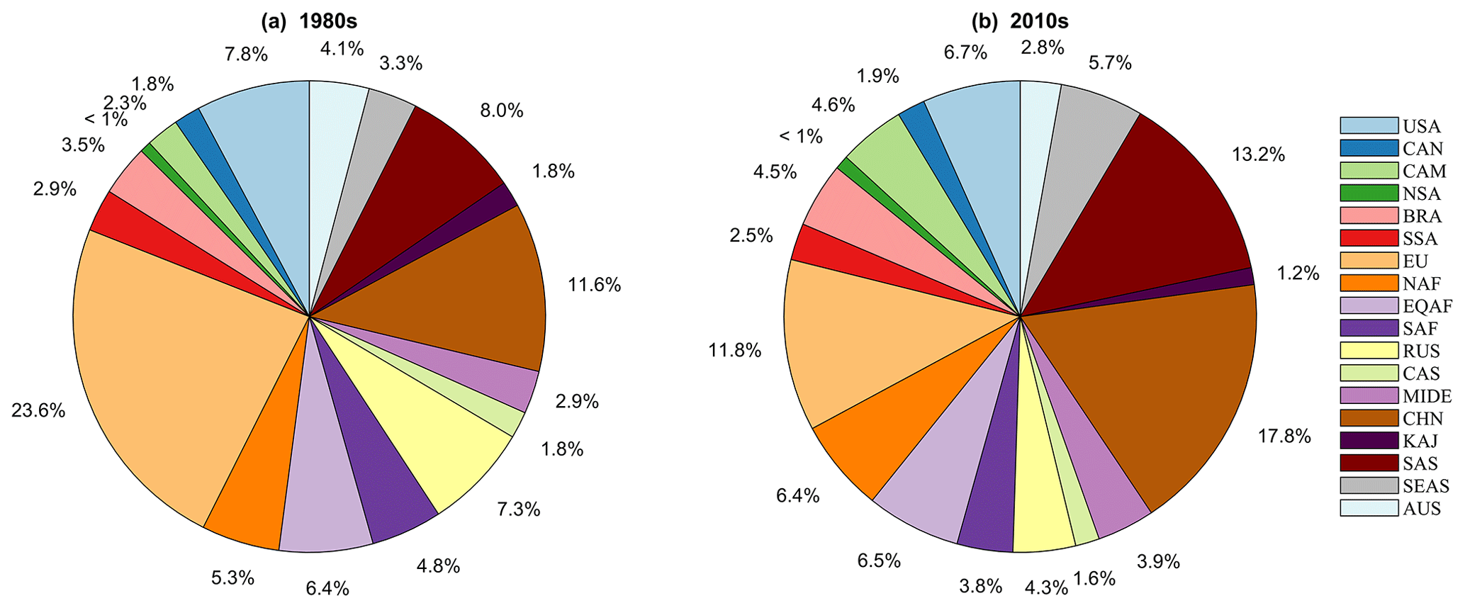
Figure 17Contributions of the 18 regions to global anthropogenic N2O emissions in the 1980s (a) and 2010s (b).
Among the 18 regions identified in this study, only Europe, Russia, Australasia, and Japan and Korea had decreasing N2O emissions. Europe had the largest rate of decrease, with an average of Tg N yr−2 during 1980–2020 (31 % reduction), largely resulting from reduced emissions from fossil fuel and industry, which changed from 0.49 Tg N yr−1 in 1980 to 0.14 Tg N yr−1 in 2020. In addition to the large reduction in fossil fuel and industry emissions in Europe, direct agricultural emissions and indirect emissions showed overall decreasing trends from 0.46 and 0.16 Tg N yr−1 in 1980 to 0.38 and 0.12 Tg N yr−1 in 2020, respectively. However, the decreasing trend in agricultural emissions has leveled off since the 2000s.
China and South Asia had the largest increase in N2O emissions during the study period. The rates of increase in the anthropogenic emissions from China and South Asia were and Tg N yr−2, respectively. The rates of increase in the anthropogenic emissions from China and South Asia contributed 40 % and 30 % to the global anthropogenic increase rate (0.05 Tg N yr−2), respectively. In these two regions, direct nitrogen additions in agriculture made the largest contribution, while other direct emissions and indirect emissions also steadily increased. Our results show a significant increase in anthropogenic N2O emissions from South America, which is consistent with the previous budget (Tian et al., 2020). Moreover, we reveal that Brazil had a higher increase rate in anthropogenic N2O emissions ( Tg N yr−2) than northern South America ( Tg N yr−2) and southwestern South America ( Tg N yr−2) during 1980–2020, and direct emissions from agriculture made the largest contribution. Our results suggest that northern Africa made the largest contribution (58 %) to the increase in anthropogenic N2O emissions from Africa, followed by equatorial Africa (38 %) and southern Africa (4 %). Anthropogenic N2O emissions from the USA and Canada show similar weak increasing rates of and Tg N yr−2 during the 1980–2020 period, respectively. Central America shows a higher anthropogenic N2O emission increase rate ( Tg N yr−2), which is attributed to an increase in emissions from fossil fuels and industry, from 0.01 Tg N yr−1 in the 1980s to 0.16 Tg N yr−1 in the 2010s. The data for Mexico from EDGAR have a known problem with their estimates of N2O emissions from industry, and this issue requires further exploration. To support countries' N2O mitigation, it is essential to accurately estimate sources and sinks of N2O at the national level.
6.2 Sources of uncertainties and suggestions for improvements
6.2.1 Uncertainties in N2O emission factors
Four inventories of N2O emissions (EDGAR, FAOSTAT, GFED, and UNFCCC) are integrated into the current synthesis of anthropogenic N2O emissions. These EF-based inventory datasets (where EF refers to emission factors) used the IPCC default EFs at regional and global scales. Uncertainty in FAOSTAT N2O emissions is ∼60 % across typologies. In fact, it is asymmetrical, following the 2006 guideline values and IPCC uncertainty formulae, with % and umax∼90 % (Tubiello et al., 2013); for N2O in EDGAR, the global uncertainty ranges defining the 95 % confidence intervals of a lognormal distribution are ±113 % for energy, between −12 % and +16 % for industrial processes and product use, between −225 % and +302 % for agriculture, between −159 % and +203 % for waste, and ±112 % for other sectors (Solazzo et al., 2021). However, the poorly captured dependence of EFs on regional climate, management practices such as tillage, legume effect, and soil physical and biochemical conditions are key causes of the large uncertainty in the estimates of agricultural N2O emissions (Shcherbak et al., 2014; Tian et al., 2019; Lu et al., 2022), particularly for croplands where EFs have high spatial heterogeneity (Shang et al., 2019; Wang et al., 2020). There is evidence of a greater-than-linear dependence of emissions on N input where there is an excess of N; however, this is not represented in inventories that assume a linear dependence on N input (Cui et al., 2021). Higher IPCC-tier GHG inventories using the alternative EFs that are disaggregated by environmental factors and management-related factors (Buendia et al., 2019) could provide more accurate estimates, especially for regions where N input surplus is high, such as eastern China, India, and the USA. For example, the US national inventory uses a Tier-3 modeling approach (Del Grosso et al., 2022). Establishing national and regional N2O flux measurement networks could improve the accuracy of EF estimates for regions with different vegetation types and management measures. Furthermore, inventory datasets based on EF methods also suffer from large uncertainties induced by the underlying agriculture and rural data and statistics used as input, including statistics on fertilizer applications, livestock manure availability, storage and applications, and nutrient, crop, and soil management.
According to the ensemble of process-based land model emissions derived from NMIP2, we estimate that the EF of fertilizer and manure applied on global croplands was 1.9 % (1.2 %–3.3 %) in the 2010s, which is significantly larger than the IPCC Tier-1 default for direct emission of 1 %. This higher EF derived from process-based models suggests a strong interactive effect between N additions and other global environmental changes (Perturbed fluxes from climate, atmospheric CO2, and land-cover change in Table 3). Figure 18 shows the spatial pattern of the cropland N2O EF during the 2010s and highlights that the EF was high in eastern China, Southeast Asia, western Europe, and the central USA where anthropogenic N inputs were high (Fig. B3). Previous field experiments reported a better fit to local observations of soil N2O emissions when assuming a nonlinear response to fertilizer N inputs under varied climate and soil conditions (Shcherbak et al., 2014; Wang et al., 2020). The nonlinear response is also likely associated with long-term N accumulation in agricultural soils from N fertilizer use and in aquatic systems from N loads (the legacy effect) (Van Meter et al., 2016), which provides more substrate for microbial processes (Firestone and Davidson, 1989). The increasing N2O emissions estimated by process-based models (Tian et al., 2019) also suggest that recent climate change (particularly warming) may have boosted soil nitrification and denitrification processes, contributing to the growing trend in N2O emissions with rising N additions to agricultural soils (Griffis et al., 2017; Pärn et al., 2018; Smith, 1997).

Figure 18Spatial pattern of the emission factor (EF) of fertilizer and manure applied on global croplands in the 2010s derived from NMIP2.
6.2.2 Uncertainties in estimates of soil N2O emissions
Both process-based land biosphere modeling and measurement-based upscaling approaches have been used to estimate global soil N2O emissions (Table 3), with large uncertainties in their estimates. As shown in Fig. 19, NMIP2 models exhibit the highest uncertainties in the estimates of soil N2O emissions from tropical forests, such as the Amazon Basin, the Congo Basin, and Southeast Asia, as well as in regions with high fertilizer application rates, including eastern China, northern India, and the US Corn Belt. For NMIP2 estimates of direct agricultural emissions, the maximum estimate is about 60 % higher than the ensemble mean, and the minimum estimate is about 40 % lower than the ensemble mean. A large discrepancy in natural soil emissions among NMIP2 models exists, ranging from 3.9 to 8.6 Tg N yr−1, which needs to be reconciled in future research.

Figure 19Spatial distribution of uncertainty (1 standard deviation) in NMIP2 estimations of soil N2O emissions in the 2010s.
Uncertainties associated with NMIP2 models
The uncertainties in process-based models primarily stem from differences in model configuration and process parameterization as well as from the missing processes and critical information (Tian et al., 2019).
First, the NMIP2 models use divergent schemes to represent the flows of reactive N through ecosystems (biological N fixation, N deposition, N leaching, N volatilization, nitrification, and denitrification), which could result in large discrepancies in soil mineral N that serves as substrates for N2O production. Explicit representation of these processes is a critical need with respect to enhancing model simulation accuracy.
Second, several important processes are missing in most process-based land models. Human management measures like tillage and legume cultivation can alter the physical and chemical characteristics of soil in croplands (Raji and Dörsch, 2020; Z. Yu et al., 2020), but they are not adequately represented in most NMIP2 models. Parameterizing these processes in the models is necessary to reduce uncertainty. Additionally, N addition in pasture and rangeland (e.g., livestock excreta deposition, manure, and mineral fertilizer application) constitutes an important source of global soil N2O emissions (Davidson, 2009), accounting for more than half of the global agricultural N2O emissions (Dangal et al., 2019). However, only DLEM considered these processes. The consideration of N addition in managed grasslands is an essential task for process-based models to estimate grassland soil N2O emissions accurately. Moreover, most process-based models did not explicitly consider seasonal freeze–thaw processes or the thawing of permafrost, which can emit substantial amounts of N2O (Marushchak et al., 2011, 2021; Repo et al., 2009; Voigt et al., 2017; Del Grosso et al., 2022). It is recommended to include explicit representation of permafrost physics and seasonal freeze–thaw processes in process-based models, as this would help better catch the “hotspot” and “hot moment” of soil N2O emissions in northern regions (Wagner-Riddle et al., 2017). Current process-based models also face challenges in adequately representing the fine-grained landscape structure of Arctic ecosystems (e.g., landscape elements that act as ultra-emitters of N2O, like organic soil non-vegetated fractions); thus, integrating sub-grid information and processes into models may provide a solution for fine-grained physical–hydrological modeling.
Third, microbial nitrification and denitrification processes are regulated by multiple environmental factors, including substrate availability, precipitation, temperature, oxygen status, pH, vegetation type, and atmospheric CO2 concentration (Butterbach-Bahl et al., 2013; Dijkstra et al., 2012; Li et al., 2020; Tian et al., 2019; Yin et al., 2022; Yu et al., 2022). However, there is significant divergence among NMIP2 models in their response to these factors. For example, simulated soil N2O emissions in response to N addition (i.e., fertilizer and manure N applications and N deposition) exhibit large divergence among the participating NMIP2 models, primarily due to differences in model representation of N processes and parameterization schemes. Moreover, in contrast to our findings indicating N fertilizer application and manure additions as dominant drivers, Harris et al. (2022) identified N deposition as the primary contributor to anthropogenic N2O emissions, accounting for 41±14 % of all anthropogenic emissions. These different findings highlight the complex nature of N2O emissions and the need for further research to better understand the relative contributions of different N sources. For the climatic effects on soil N2O emissions, our NMIP2 models indicate enhanced N2O emissions due to warming, consistent with findings from experiment-based studies (Smith, 1997; Cui et al., 2018; Voigt et al., 2017; Wang et al., 2017), as the denitrifying bacteria community may adapt to higher temperature (Pärn et al., 2018). Additionally, considering that microbial nitrification and denitrification are also largely controlled by soil moisture (Butterbach-Bahl et al., 2013), it is important to address the discrepancies in NMIP2 models concerning soil moisture representation, such as soil depth, root distribution, root water uptake, and water movement processes (Ostle et al., 2009; Raats, 2007; Raoult et al., 2018).
At the global scale, although NMIP2 models show large discrepancies in the CO2 effect on soil N2O emissions, most NMIP2 models show a negative effect, suggesting that enhanced plant N uptake caused by a rising CO2 concentration played a dominant role (Usyskin-Tonne et al., 2020; Tian et al., 2019). Nevertheless, observation-based results of the CO2 effect diverge among different ecosystem types, with some studies reporting reduced N2O emissions in forests under elevated CO2 (Phillips et al., 2001), while others found increased emissions in grasslands (Moser et al., 2018; Regan et al., 2011). It should be noted that the interactions among environmental factors influencing soil N2O emissions are still poorly represented in the NMIP2 models. Further targeted continuous measurements and manipulation experiments are needed to better represent the interactive effects of multiple environmental factors on N2O emissions in the models to improve the simulation of complex N2O dynamics. Finally, simulations targeted to explain the reconstructed increase in terrestrial N2O emissions over the deglaciation and during past abrupt climate events will further help to constrain process-based models (Fischer et al., 2019; Joos et al., 2020).
Land-cover change/deforestation
The two methods for estimating deforestation-induced N2O changes have their limitations. The accuracy of the empirical estimates of post-deforestation pulse N2O emissions in tropical forests strongly depends on the availability of paired N2O observations in deforested and nearby intact forest sites (Melillo et al., 2001; Verchot et al., 1999), which are extremely scarce. Moreover, a fixed value was adopted as the default reference N2O emission rate for tropical forests to simplify computation, but it inevitably ignored the spatiotemporal heterogeneity in tropical forest N2O emissions (Barthel et al., 2022). It is also noted that there were no empirical post-deforestation N2O emission estimates in extra-tropical areas, as no feasible empirical relationships between N2O emissions and years after deforestation were available. The accuracy of process-based estimates (specifically by DLEM here) could be regulated by model-specific configurations for land-use change pathways. For example, in modeling tropical shift cultivation, DLEM assumed that agricultural lands newly converted from forests can only be reforested after at least 15 years to be consistent with the LUHv2 data (Hurtt et al., 2020). Meanwhile, treatments of different nitrogen pools (such as leaf, stem, root, and litter pools) during land conversion would directly influence the nitrogen substrate for nitrification and denitrification. The DLEM model follows the biomass allocation scheme proposed by previous studies (Houghton et al., 1983; McGuire et al., 2001), which may introduce uncertainty in varied land management practices. A bias in the LUHv2 land-use change data in regions experiencing drastic land conversions could also contribute to uncertainty in deforestation-induced GHG emissions, for example, in areas with large-scale plantations (Yu et al., 2022).
In addition, developing forcing datasets with high quality and high spatiotemporal resolution is also important for reducing uncertainties in simulated N2O fluxes. Among various input variables, precise information regarding fertilizer and manure application (including crop-specific application rate, type, timing, and frequency) is pivotal for improving the accuracy of model simulations. However, this crucial information was not unified in NMIP2 simulations, leading to increased modeling uncertainty. To mitigate this issue, it is strongly recommended to use improved fertilizer and manure datasets that provide detailed information on crop-specific application rate, timing, and frequency to drive models in future intercomparison projects. Moreover, with the availability of additional high-precision datasets from manipulation field experiments (e.g., microbial data), we could use these datasets to constrain our models and delve deeper into the underlying mechanisms that regulate N2O fluxes (e.g., the role of soil microbes) and further incorporate these mechanisms into models to reduce uncertainties.
Uncertainties associated with the measurement-based upscaling approach
Measurement-based upscaling estimates are subject to uncertainties due to various factors. One major reason is the limited recording of microscale variables and the incomplete quantification of local EFs related to microbial N2O production. Sampling limitations also contribute to uncertainties, as the frequency and repeatability of measurements may not fully capture the high spatiotemporal variability in the N2O flux. The lack of the history of control sites further complicates the exclusion of observation data with significant legacy fluxes, thereby biasing our estimates. Additionally, gaps in global agricultural management datasets, particularly regarding fertilization details, enlarge the prediction interval of EFs and introduce uncertainties. We then used a Monte Carlo simulation to estimate three sources of uncertainty for predicting EFs based on a flux upscaling approach: (i) the fixed coefficients, (ii) the random coefficients, and (iii) input data. The uncertainty from sampling frequency and replication is reflected in the first source, while the uncertainty from unquantified sources related to field measurements is reflected in the second source. Each of the crop-specific SRNM models was run by randomly generating the fixed and random coefficients from their fitted multivariate normal distribution as well as climate, soil, and other relevant factors following independent normal distributions with the mean of the value in our dataset and standard deviation of the absolute difference between the dataset used in this study and other global datasets. Fertilizer frequency was randomly selected using a Bernoulli distribution. Predicted values were calculated through 1000 iterations to construct a 95 % prediction interval. The breakdown of uncertainty revealed that the random coefficients contributed the most to the estimation uncertainty, with observations showing that they explained more variance in EFs compared with fixed effects (47 %–74 % versus 19 %–35 %) and contributed to most of estimation uncertainty (Fig. 20).
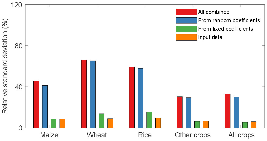
Figure 20Relative standard deviation in the global cropland N2O EF. The figure breaks down the uncertainty in the EF per source of uncertainty (i.e., random coefficients, fixed coefficients, input data, or all combined). The uncertainty due to each source can be quantified by holding the coefficients for the other sources fixed.
To address these limitations and reduce uncertainties, concerted efforts should be made to enhance the availability of N2O observations representing diverse agroecological conditions. Meanwhile, improving the availability of high-precision datasets (e.g., microbial data) and integrating these datasets and the derived underlying mechanisms to our models could also reduce uncertainties. Currently, most available field N2O observations (see the Supplement) are made in Europe, the USA, and China and are scarce in most developing countries (such as sub-Saharan Africa). Therefore, extending the global coverage of direct and indirect N2O flux measurements to encompass all major agricultural land-use types and climates, land-use changes, and management practices as well as conducting long-term high-frequency monitoring are particularly important to increase the reliability of EFs as well as upscale results from site to regional scales.
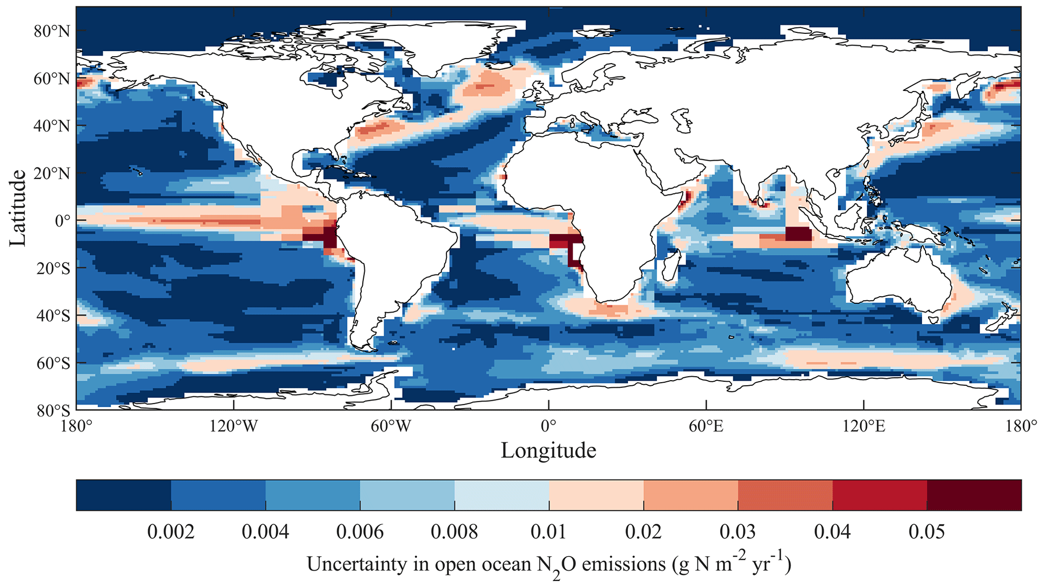
Figure 21Spatial uncertainty distribution (1 standard deviation) in open-ocean N2O emissions in the 2010s. Note that the color scale in this figure is different from that in Fig. 19.
6.2.3 Uncertainties in estimates of ocean N2O emissions
Global open-ocean N2O emissions derived from the ocean biogeochemistry models (Table 1) for the 2010–2019 period are estimated to be 3.5 (2.5–4.7) Tg N yr−1. All models show the highest emissions associated with equatorial and coastal upwelling zones as well as with the major oxygen minimum zones (OMZs; e.g., the eastern equatorial Pacific and the Arabian Sea region of the northern Indian Ocean; see Fig. 21). These are regions characterized by high levels of biological productivity and higher subsurface organic matter remineralization, resulting in higher N2O yields in suboxic waters. The four participating models capture these characteristics but also show varying degrees of intensity in regional N2O emissions. The models also show good agreement with respect to representing the ocean regions of relatively low N2O ocean–atmosphere fluxes (i.e., open-ocean gyres where biological productivity is low).
The spatial distribution of uncertainty in ocean N2O emissions among the models (Fig. 21) is similar to that of the net N2O ocean–atmosphere flux, with the highest uncertainties observed in the equatorial upwelling and low-oxygen waters associated with high subsurface N2O production (Babbin et al., 2020; Ganesan et al., 2020). The largest uncertainties are found in the equatorial Pacific, the Benguela upwelling region of the Atlantic, and the eastern equatorial Indian Ocean. Uncertainties in the ocean models' representation of N2O fluxes result from a range of model characteristics (Zamora and Oschlies, 2014; Martinez-Rey et al., 2015; Buitenhuis et al., 2018; Battaglia and Joos, 2018; Landolfi et al., 2017; Berthet et al., 2023), including the following: (i) uncertainties in ocean circulation – particularly the representation of upwelling zones and the ocean circulation features (often sub-grid scale) that control the extent and intensity of OMZs; (ii) simulation of ocean organic matter productivity, export production, and mesopelagic remineralization (a driver of the subsurface source function for N2O production in models); (iii) the model biogeochemical parameterizations representing N2O production and consumption from marine nitrification and denitrification processes, including their dependence on local dissolved oxygen concentrations and thresholds; and (iv) parameterization of ocean–atmosphere gas-exchange fluxes.
Model simulations of oceanic N2O are closely linked to the underlying modeled oxygen distributions, as the embedded biogeochemical parameterizations for N2O include the sensitivity of N2O cycling processes (e.g., nitrification and denitrification) to the local oxygen level (Ji et al., 2018). Significant uncertainties in modeled N2O fluxes result from model biases in the representation of dissolved oxygen, especially in low-oxygen zones such as the eastern equatorial Pacific (Zamora and Oschlies, 2014; Martinez-Rey et al., 2015). Many ocean model simulations of dissolved oxygen display biases, especially in OMZs critical for N2O cycling (Martinez-Rey et al., 2015). To reduce potential sources of error from model-simulated oxygen, one N2O model in this analysis employs observation-based oxygen distributions when simulating ocean N2O (Buitenhuis et al., 2018). However, this approach also restricts a model's response to climate-related feedback on ocean oxygen. In addition, the models in this analysis include optimization and calibration of N2O cycle parameters by incorporating constraints from ocean observations (e.g., surface and interior N2O and microbially mediated process rates) (Battaglia and Joos, 2018; Buitenhuis et al., 2018; Berthet et al., 2023). A more detailed error analysis of N2O model parameters (including uncertainty in gas-exchange fluxes) in one of the component models (Buitenhuis et al., 2018) suggests estimated uncertainties in global fluxes from biogeochemical parameter specifications of ∼33 %. Further, a 1000-member ensemble with 11 parameters varied with one of the models and constrained with both surface and subsurface N2O observations yields an observation-constrained standard deviation of ±36 % around the median of 4.3 Tg N yr−1 (Battaglia and Joos, 2018), consistent with a recent surface pN2O-based estimate of 4.2±1 Tg N yr−1 (Yang et al., 2020).
Landolfi et al. (2017) also note that uncertainties arise in current model predictions of marine N2O fluxes due to the neglect of feedback from impacts of external nutrient sources and ocean acidification on marine productivity and the ocean nitrogen and oxygen cycles. Reducing uncertainties in model estimates of the evolution of ocean N2O fluxes will require accounting for these impacts in the underlying biogeochemical parameterizations. In addition, due to the high sensitivity of modeled N2O production and consumption rates to oxygen level in the key ocean OMZ zones, an important priority in reducing modeled ocean N2O flux uncertainties is to achieve a more accurate simulation of the ocean circulation and oxygen distribution of these regions.
6.2.4 Uncertainties in emissions estimates from the continental shelves
Estimates of N2O emissions vary by a factor of 2–3 in the continental shelf (one observation-based product and two models). The MEM-RF observational estimate (1.63 Tg N yr−1; Yang et al., 2020) falls at the high end of the two high-resolution model estimates (1.39 and 0.61 Tg N yr−1 for CNRM-0.25° and ECCO-Darwin, respectively). Shelf N2O flux emissions from MEM-RF, CNRM-0.25°, and ECO-Darwin broadly agree with respect to the main patterns and magnitude. Emission hotspots in productive, low-O2 upwelling systems (e.g., eastern boundary upwellings and upwellings of the northwestern Indian Ocean) appear to be underestimated by models. Lower emissions in models likely reflect the inability of models to resolve complex near-shore dynamical circulation and biogeochemical processes key to the production, transport, and evasion of N2O. This includes under-resolved dynamics in upwelling systems and shallow OMZs with high N2O emissions (Resplandy et al., 2024), strong spatial gradients introduced by patterns of high production/high remineralization and enhanced land–sea inputs of N in shallow shelves (e.g., Baltic Sea as well as Southeast and East Asia), sedimentary processes, and production in estuarine and coastal vegetated ecosystems, which is subsequently transported offshore. Conversely, our ability to reconstruct spatial patterns in N2O air–sea fluxes from observations (MEM-RF; Yang et al., 2020), in particular along continental margins, is severely limited by the number of N2O observations, which is 2 orders of magnitude smaller than for CO2. Observations tend to be localized in regions of strong air–sea disequilibrium and, thus, might be biased high (e.g., Babbin et al., 2020; Ganesan et al., 2020). In addition, many coastal regions remain undersampled, further limiting the performance of MEM-RF. For instance, models point to coastal N2O flux hotspots along midlatitude western boundaries (e.g., the US East Coast, the North Pacific east of Japan, the southeast coast of Australia, and the southeastern tip of Africa) that are not diagnosed in the observational product (Resplandy et al., 2024). Furthermore, N2O fluxes are highly spatially heterogeneous (scales of 1 to 100 km) due to land–ocean gradients and mesoscale and sub-mesoscale features such as eddies (Arévalo-Martínez et al., 2017, 2019; Yang et al., 2020; Grundle et al., 2017). Eddies are instrumental in setting suboxic conditions favorable for N2O production, and it has been suggested that N2O production weakens within eddies during their transit across the shelf and further offshore (Arévalo-Martinez et al., 2016). These small-scale circulation features are important controls on N2O dynamics but are poorly accounted for in data-based reconstructions and models.
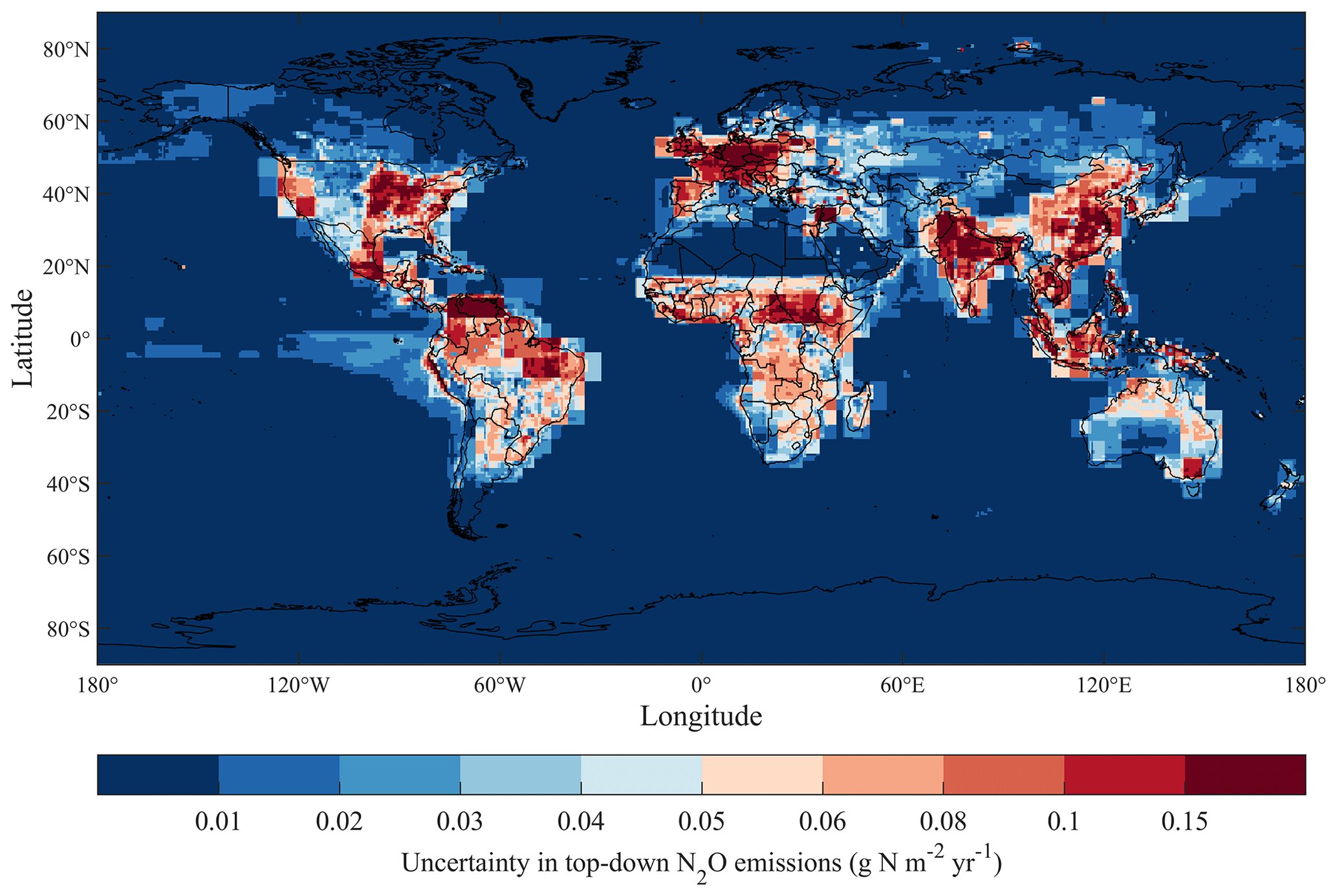
Figure 22Spatial distribution of posterior uncertainty (1 standard deviation) in TD model estimates of N2O emissions in the 2010s.
This assessment provides the most up-to-date estimate of N2O climatological emissions from the global shelves, but the variability in these emissions remains uncertain. Each product covers a different time period and only provides limited or missing information on seasonal fluctuations, interannual variability, and long-term trends. For instance, only a handful of observations per year are available in most regions, providing a limited picture of seasonality and even more limited information on interannual variability (e.g., El Niño–Southern Oscillation and Pacific Decadal Oscillation) and global longer-term trends. Disentangling such influences from limited observations alone remains a major challenge. The effects of extreme events, such as storms and marine heat waves, on N2O fluxes are also currently not captured, and the intra-annual variability in hotspot regions, such as coastal upwelling systems, remains poorly constrained. Despite these limitations, data-based reconstructions and models suggest a vigorous seasonal cycle and, potentially, important variability on interannual timescales (Yang et al., 2020; Ganesan et al., 2020). The development of a global N2O ocean observation network (N2O-ON; Bange et al., 2019; Bange, 2022) is critically needed to better resolve spatiotemporal patterns and reduce uncertainties in N2O emissions. Increasing the density of observations in regions of high N2O disequilibrium and collecting long time series of N2O measurements will allow for better characterization of interannual changes and their dynamics. Meanwhile, algorithmic approaches that address the observational limitations should be developed and refined to extrapolate N2O measurements to global and interannual timescales, leveraging advancements made for CO2 disequilibrium and flux reconstructions.
Parallel efforts based on the development of mechanistic models are also needed to strengthen our understanding of the dynamics underlying interannual N2O flux variability and to detect and attribute long-term anthropogenic effects. However, the representation of N2O processes in biogeochemical models remains limited, and very few climate models include marine emissions of N2O fluxes (only 4 out of 26 CMIP6 models considered in Séférian et al., 2020). Uncertainty persists regarding the various (micro-)biological processes that drive N2O cycling in coastal waters and sediments (Bange, 2022). Current global ocean biogeochemical models typically adopt an indirect representation of N2O production, which is diagnosed from environmental conditions (e.g., temperature) and O2 consumption during remineralization of organic matter, without explicitly representing the bacterial pools and chemical reactions responsible for N2O production in suboxic waters (e.g., Aumont et al., 2015; Battaglia and Joos, 2018). In addition, key aspects of air–sea N2O exchange, such as the effects of surfactants in the sea surface microlayer (Kock et al., 2012), remain poorly understood. Finally, the interannual variability in N2O fluxes and its attribution to climatic and anthropogenic drivers is largely unknown. Disentangling these influences will benefit from (1) interannually varying observational N2O flux reconstructions at scales fine enough to capture high emissions along continental margins, (2) statistical methods that address the limited number of observations in space and time, and (3) N2O cycle simulations with forward mechanistic models. A blueprint for this work already exists with the approaches developed by the oceanic CO2 community (Gruber, 2022). Similar approaches would enable attribution of N2O flux changes to specific drivers, leading to better predictability.

Figure 23Uncertainty reduction (1 – sigma_posterior/sigma_prior) from the PyVAR-CAMS inversion framework. Asterisks (*) represent atmospheric observational stations used in the inversion framework.
6.2.5 Uncertainties in emissions estimates from atmospheric inversions
The four atmospheric inversion frameworks show uncertainties in the estimates of N2O emissions, especially in hotspot regions such as eastern China, India, Europe, the US Corn Belt, and northern South America (Fig. 22). The uncertainties in inversion estimates are mainly from errors in the modeled atmospheric transport, the dependence on the prior information, and the availability of atmospheric observations. Every inversion framework in this study used a different atmospheric transport model with different horizontal and vertical resolutions (Table 1). By including estimates from multiple inversion frameworks with different modeled atmospheric transport, the systematic error can be assessed to some extent. The inversion estimates are dependent on the spatial pattern and magnitude of the prior flux estimates to an extent that is determined by the density of the observations. Using the same prior information might reduce the range in the atmospheric inversion estimates but not the uncertainty, as this depends on the spatiotemporal density of the atmospheric observations and the accuracy of the modeled transport. The uncertainty reduction (calculated as 1 minus the ratio of the posterior to prior uncertainty) indicates the degree of constraint on the inversion estimates (Fig. 23). It shows that the areas of South America, Africa, central and southern Asia, and Australasia are poorly constrained by observations. The relatively sparse distribution of current N2O observation sites underscores the necessity of establishing more sites and regular aircraft profiles, especially in tropical and subtropical regions, to better constrain inversion models and to further reduce the posterior uncertainty.
6.2.6 Other missing fluxes
We recognize that N2O emissions contributed by termites could be a significant natural source in tropical and subtropical ecosystems (Brümmer et al., 2009; Miambi et al., 2022). The metabolic activity of microbial symbionts in the termite gut can maintain steep oxygen gradients, which facilitates nitrification and denitrification processes and the production of N2O (Brauman et al., 2015; Brune et al., 1995). Nevertheless, termites have a wide trophic diversity, and their N2O emission rates vary significantly, with some species creating emission hotspots (Brümmer et al., 2009), while others function as net sinks (Majeed et al., 2012). Feeding habits and the abundance of nitrifiers and denitrifiers in the gut are reported to be the key factors determining net N2O emission of termites (Brauman et al., 2015; Miambi et al., 2022). Termites that consume N-rich material, such as soil organic matter and fungi, exhibit high N2O production rates and emit N2O into the atmosphere, while those feeding on N-deficient wood can consume atmospheric N2O (Brauman et al., 2015). It is difficult to scale up calculations of net N2O emission by termites due to the lack of data on their abundance and biomass across global ecosystems; therefore, our understanding of the precise contribution of termites to the atmospheric N2O budget on a global scale remains limited, and it is not considered in our analysis.
Table A1Comparison of terminologies used in this study and previous reports.


Table A3The sectors in the N2O budget and its sources. (An asterisk denotes that a sector only includes the maximum, mean, and minimum.)
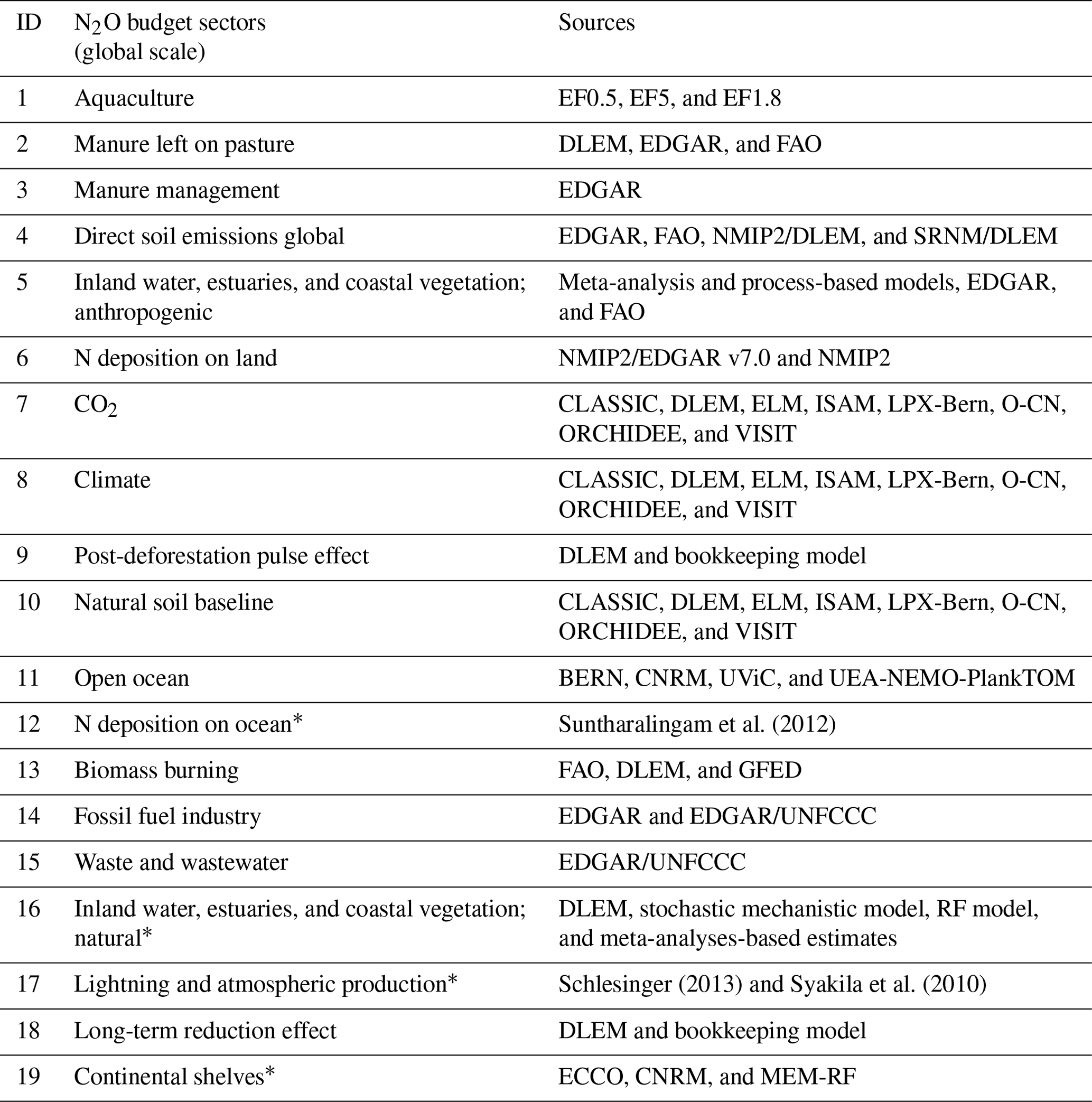
Table A4Funding supporting the production of the various components of the global nitrous oxide budget in addition to the authors' supporting institutions (see also Acknowledgements).
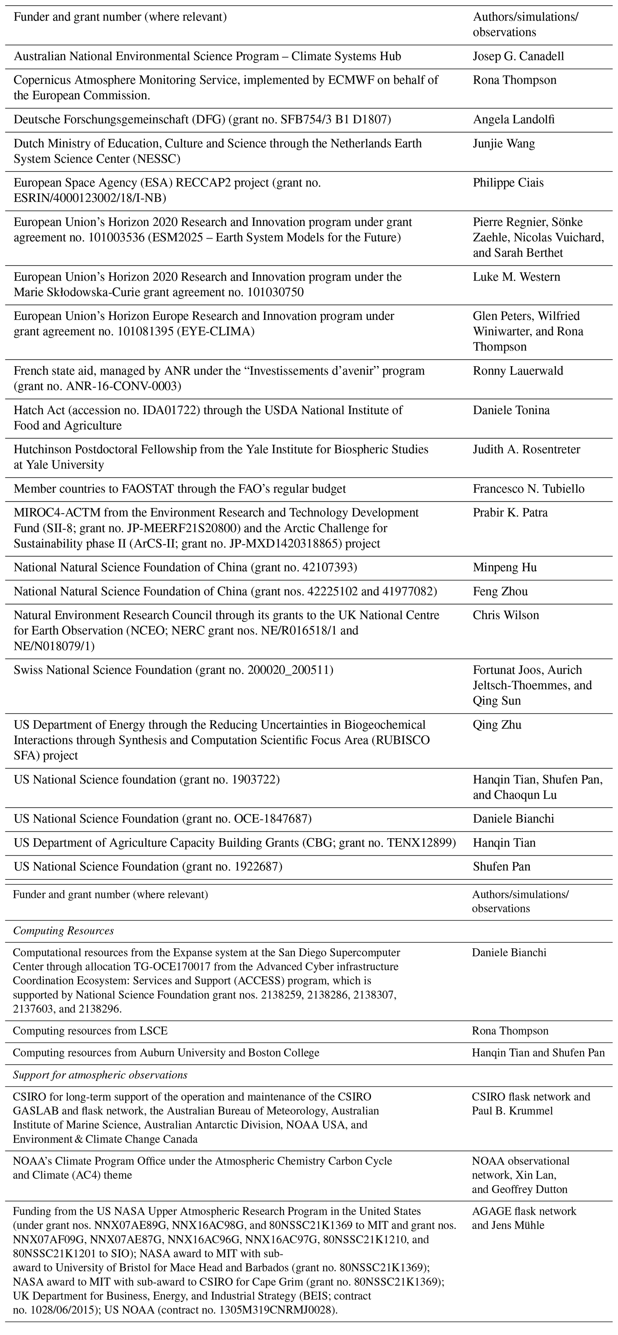

Figure B1Spatial distribution of global N2O emissions in the 2010s estimated by different atmospheric inversion frameworks (TD approach).
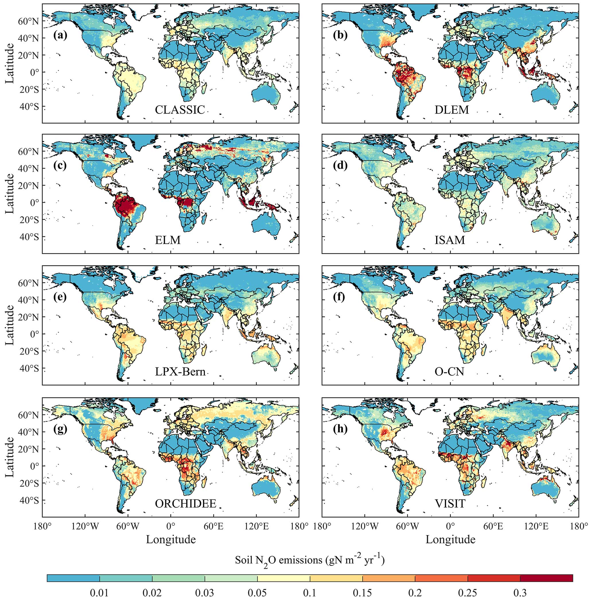
Figure B2Spatial distribution of preindustrial (1850s) soil N2O emissions estimated by different NMIP2 terrestrial biosphere models.

Figure B3Spatial–temporal changes in fertilizer N and manure N applications as well as atmospheric N deposition to global terrestrial ecosystems derived from the HaNi dataset (Tian et al., 2022), which were used to drive NMIP2 terrestrial biosphere models.
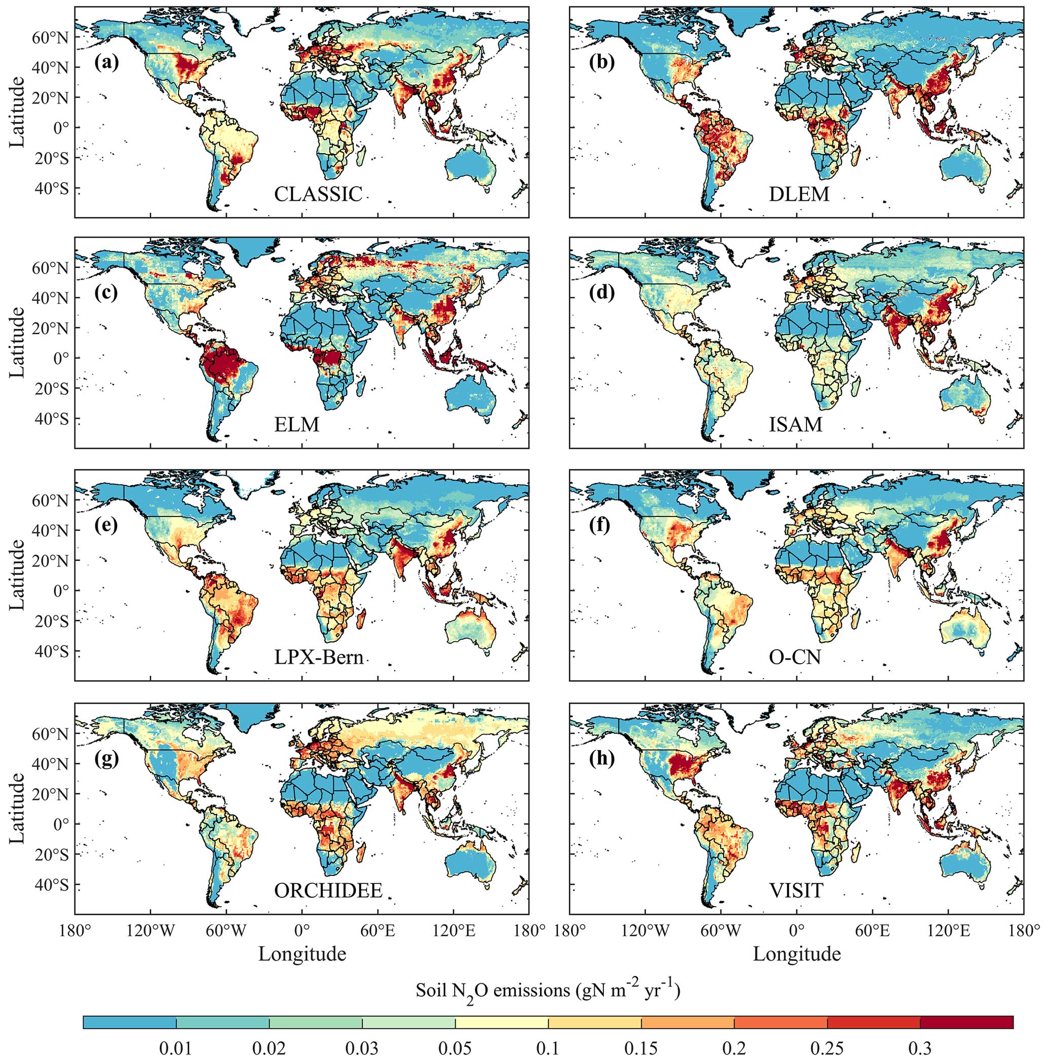
Figure B4Spatial distribution of soil N2O emissions during 2010–2019 estimated by NMIP2 terrestrial biosphere models.
Figure B5Spatial distribution of N2O emissions from open oceans during 2010–2019 estimated by different ocean biogeochemistry models and Earth system models.
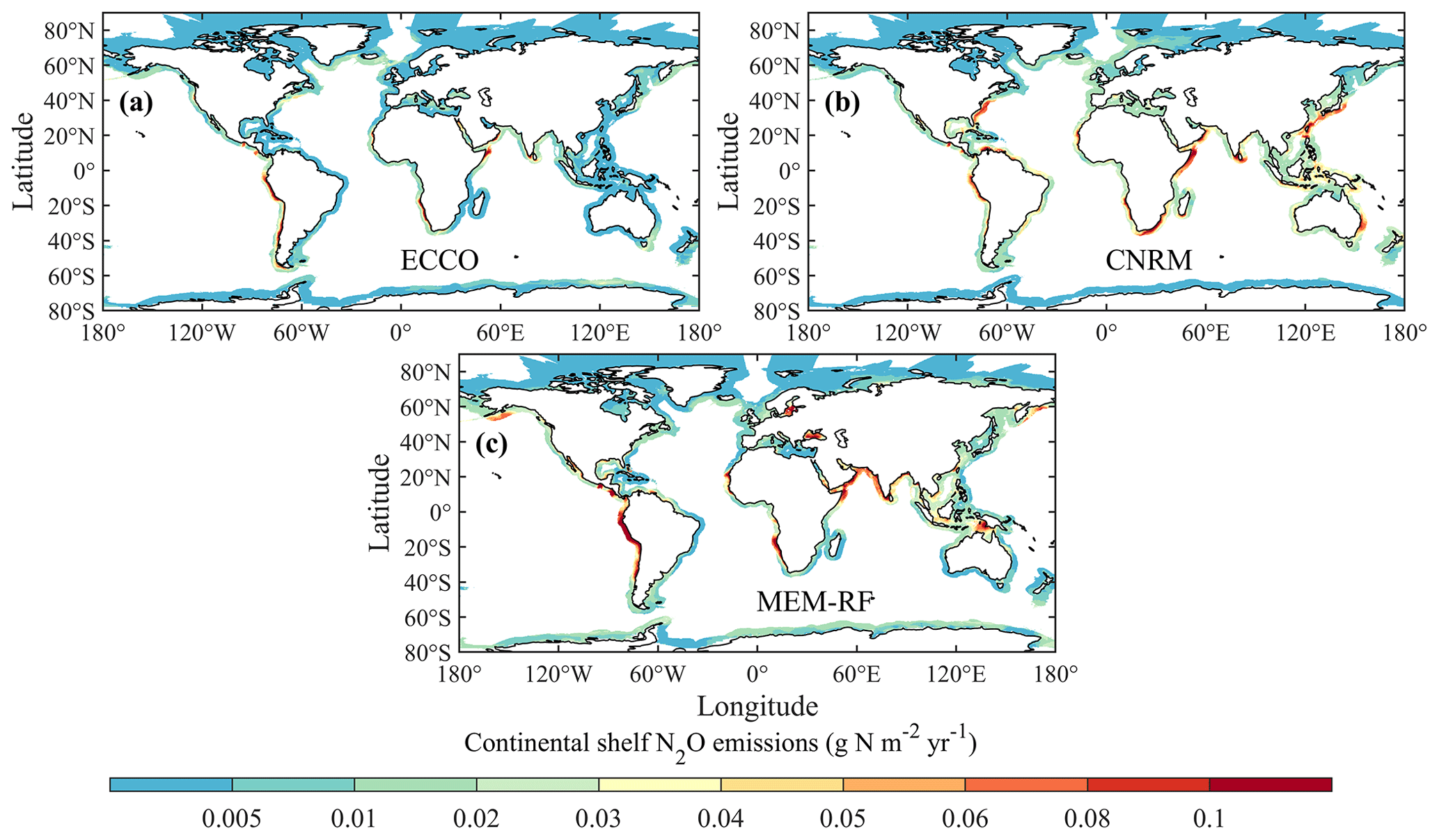
Figure B6N2O emission from continental shelves as estimated by three methods.
The supplement related to this article is available online at: https://doi.org/10.5194/essd-16-2543-2024-supplement.
HT, RLT, and JGC designed and coordinated the study. HT, NP, SP, YL, RLT, PS, and PR gathered the bottom-up and top-down datasets and performed the post-processing, analysis, and synthesis. HT, NP, RLT, JGC, PS, PR, EAD, MJP, PC, MM, SP, WW, SZ, FZ, and RBJ wrote the paper. RLT led atmospheric inversions, teaming with PKP, KCW, DBM, and CW; HT led land biosphere modeling, teaming with NP, SP, SZ, AI, AKJ, FJ, SKG, CL, HS, QS, and QZ; PS led ocean biogeochemical modeling, teaming with EB, AL, SB, AJT, and FJ; PR led the synthesis of LOAC (Land–Ocean Aquatic Continuum), teaming with RL, TM, YY, MH, PR, JR, LR, MM, SB, HB, DB, and HT; JW and LB provided the N2O flux from aquaculture data. GRW and JY provided the N2O emissions from biomass burning data. FZ provided cropland N2O flux data from a statistical model and field observations. MM, FNT, and WW provided N2O inventory data. MJP provided stratospheric and tropospheric sink data. GP provided RCP and SSP scenario data and analysis. XL and GD provided a global N2O monitoring dataset of NOAA/ESRL GMD. JM and LMW provided a global N2O monitoring dataset of AGAGE stations. PK provided a global N2O monitoring dataset of CSIRO stations. All coauthors reviewed and commented on the manuscript.
At least one of the (co-)authors is a member of the editorial board of Earth System Science Data. The peer-review process was guided by an independent editor, and the authors also have no other competing interests to declare.
Publisher's note: Copernicus Publications remains neutral with regard to jurisdictional claims made in the text, published maps, institutional affiliations, or any other geographical representation in this paper. While Copernicus Publications makes every effort to include appropriate place names, the final responsibility lies with the authors.
This paper is the result of a collaborative international effort under the umbrella of the Global Carbon Project (a project of Future Earth and a research partner of the World Climate Research Programme) in partnership with the International Nitrogen Initiative (INI). We acknowledge all of the people and institutions who provided the data used in the global nitrous oxide budget as well as the institutions funding parts of this effort (see Table A4). We acknowledge the modeling groups for making their simulations available for this analysis. The PyVAR-CAMS modeling results were funded through the Copernicus Atmosphere Monitoring Service, implemented by ECMWF on behalf of the European Commission, and were generated using computing resources from LSCE. Hanqin Tian and Shufen Pan acknowledge computational and administrative support from the Center for Earth System Science and Global Sustainability, Schiller Institute for Integrated Science and Society at Boston College. Josep G. Canadell thanks the Australian National Environmental Science Program – Climate Systems Hub for supporting the GHG budget activities of the Global Carbon Project (GCP), including the global and regional N2O budget work. We are grateful to the EDGAR team (Monica Crippa, Diego Guizzardi, Edwin Schaaf, Marilena Muntean, Efisio Solazzo, Federico Pagani, and Manjola Banja) for the work needed to publish the EDGARv7.0 Global Greenhouse Gas Emissions dataset (https://edgar.jrc.ec.europa.eu/dataset_ghg70, last access: 10 February 2022). Atul K. Jain thanks Shijie Shu and Tzu-Shun Lin for their involvement in developing and analyzing the ISAM model products used here. Giulia Conchedda, Griffiths Obli-Layrea, and Nathan Wanner contributed significant efforts to the generation of fertilizer, livestock, and soil nutrient data that underlie FAO's estimates of N2O data.
Please see a full list of funders in the Appendix (Table A4).
This paper was edited by Yuyu Zhou and reviewed by Stephen Del Grosso and two anonymous referees.
Arévalo-Martínez, D. L., Kock, A., Löscher, C. R., Schmitz, R. A., Stramma, L., and Bange, H. W.: Influence of mesoscale eddies on the distribution of nitrous oxide in the eastern tropical South Pacific, Biogeosciences, 13, 1105–1118, https://doi.org/10.5194/bg-13-1105-2016, 2016.
Arévalo-Martínez, D. L., Kock, A., Steinhoff, T., Brandt, P., Dengler, M., Fischer, T., Körtzinger, A., and Bange, H. W.: Nitrous oxide during the onset of the Atlantic cold tongue, J. Geophys. Res.-Oceans, 122, 171–184, https://doi.org/10.1002/2016JC012238, 2017.
Arévalo-Martínez, D. L., Steinhoff, T., Brandt, P., Körtzinger, A., Lamont, T., Rehder, G., and Bange, H. W.: N2O Emissions From the Northern Benguela Upwelling System, Geophys. Res. Lett., 46, 3317–3326, https://doi.org/10.1029/2018GL081648, 2019.
Asaadi, A. and Arora, V. K.: Implementation of nitrogen cycle in the CLASSIC land model, Biogeosciences, 18, 669–706, https://doi.org/10.5194/bg-18-669-2021, 2021.
Aumont, O., Ethé, C., Tagliabue, A., Bopp, L., and Gehlen, M.: PISCES-v2: an ocean biogeochemical model for carbon and ecosystem studies, Geosci. Model Dev., 8, 2465–2513, https://doi.org/10.5194/gmd-8-2465-2015, 2015.
Babbin, A. R., Boles, E. L., Mühle, J., and Weiss, R. F.: On the natural spatio-temporal heterogeneity of South Pacific nitrous oxide, Nat. Commun., 11, 3672, https://doi.org/10.1038/s41467-020-17509-6, 2020.
Bange, H. W.: Non-CO2 greenhouse gases (N2O, CH4, CO) and the ocean, One Earth, 5, 1316–1318, https://doi.org/10.1016/j.oneear.2022.11.011, 2022.
Bange, H. W., Arévalo-Martínez, D. L., de la Paz, M., Farías, L., Kaiser, J., Kock, A., Law, C. S., Rees, A. P., Rehder, G., Tortell, P. D., Upstill-Goddard, R. C., and Wilson, S. T.: A Harmonized Nitrous Oxide (N2O) Ocean Observation Network for the 21st Century, Front. Mar. Sci., 6, 157, https://doi.org/10.3389/fmars.2019.00157, 2019.
Barthel, M., Bauters, M., Baumgartner, S., Drake, T. W., Bey, N. M., Bush, G., Boeckx, P., Botefa, C. I., Dériaz, N., Ekamba, G. L., Gallarotti, N., Mbayu, F. M., Mugula, J. K., Makelele, I. A., Mbongo, C. E., Mohn, J., Mandea, J. Z., Mpambi, D. M., Ntaboba, L. C., Rukeza, M. B., Spencer, R. G. M., Summerauer, L., Vanlauwe, B., Van Oost, K., Wolf, B., and Six, J.: Low N2O and variable CH4 fluxes from tropical forest soils of the Congo Basin, Nat. Commun., 13, 330, https://doi.org/10.1038/s41467-022-27978-6, 2022.
Battaglia, G. and Joos, F.: Marine N2O Emissions From Nitrification and Denitrification Constrained by Modern Observations and Projected in Multimillennial Global Warming Simulations, Global Biogeochem. Cy., 32, 92–121, https://doi.org/10.1002/2017GB005671, 2018.
Berthet, S., Séférian, R., Bricaud, C., Chevallier, M., Voldoire, A., and Ethé, C.: Evaluation of an Online Grid-Coarsening Algorithm in a Global Eddy-Admitting Ocean Biogeochemical Model, J. Adv. Model. Earth Syst., 11, 1759–1783, https://doi.org/10.1029/2019MS001644, 2019.
Berthet, S., Jouanno, J., Séférian, R., Gehlen, M., and Llovel, W.: How does the phytoplankton–light feedback affect the marine N2O inventory?, Earth Syst. Dynam., 14, 399–412, https://doi.org/10.5194/esd-14-399-2023, 2023.
Beusen, A. H. W., Bouwman, A. F., Van Beek, L. P. H., Mogollón, J. M., and Middelburg, J. J.: Global riverine N and P transport to ocean increased during the 20th century despite increased retention along the aquatic continuum, Biogeosciences, 13, 2441–2451, https://doi.org/10.5194/bg-13-2441-2016, 2016.
Bouwman, A. F., Pawłowski, M., Liu, C., Beusen, A. H. W., Shumway, S. E., Glibert, P. M., and Overbeek, C. C.: Global Hindcasts and Future Projections of Coastal Nitrogen and Phosphorus Loads Due to Shellfish and Seaweed Aquaculture, Rev. Fish. Sci., 19, 331–357, https://doi.org/10.1080/10641262.2011.603849, 2011.
Bouwman, A. F., Beusen, A. H. W., Overbeek, C. C., Bureau, D. P., Pawlowski, M., and Glibert, P. M.: Hindcasts and Future Projections of Global Inland and Coastal Nitrogen and Phosphorus Loads Due to Finfish Aquaculture, Rev. Fish. Sci., 21, 112–156, https://doi.org/10.1080/10641262.2013.790340, 2013a.
Bouwman, L., Daniel, J. S., Davidson, E. A., de Klein, C., Holland, E., Ju, X., Kanter, D., Oenema, O., Ravishankara, A. R., and Skiba, U. M.: Drawing down N2O to protect climate and the ozone layer, A UNEP Synthesis Report, UNEP – United Nations Environment Programme, https://nora.nerc.ac.uk/id/eprint/505848 (last access: 5 April 2021), 2013b.
Brauman, A., Majeed, M. Z., Buatois, B., Robert, A., Pablo, A.-L., and Miambi, E.: Nitrous Oxide (N2O) Emissions by Termites: Does the Feeding Guild Matter?, PLOS ONE, 10, e0144340, https://doi.org/10.1371/journal.pone.0144340, 2015.
Brümmer, C., Papen, H., Wassmann, R., and Brüggemann, N.: Termite mounds as hot spots of nitrous oxide emissions in South-Sudanian savanna of Burkina Faso (West Africa), Geophys. Res. Lett., 36, L09814 https://doi.org/10.1029/2009GL037351, 2009.
Brune, A., Emerson, D., and Breznak, J. A.: The termite gut microflora as an oxygen sink: microelectrode determination of oxygen and pH gradients in guts of lower and higher termites, Appl. Environ. Microbiol., 61, 2681–2687, 1995.
Buendia, E. C., Tanabe, K., Kranjc, A., Baasansuren, J., Fukuda, M., Ngarize, S., Osako, A., Pyrozhenko, Y., Shermanau, P., and Federici, S.: Refinement To the 2006 Ipcc Guidelines for National Greenhouse Gas Inventories, IPCC, Geneva, Switzerland, https://www.ipcc-nggip.iges.or.jp/public/2019rf/pdf/0_Overview/19R_V0_00_Cover_Foreword_Preface_Dedication.pdf (last access: 17 February 2020), 2019.
Buitenhuis, E. T., Suntharalingam, P., and Le Quéré, C.: Constraints on global oceanic emissions of N2O from observations and models, Biogeosciences, 15, 2161–2175, https://doi.org/10.5194/bg-15-2161-2018, 2018.
Butterbach-Bahl, K., Baggs, E. M., Dannenmann, M., Kiese, R., and Zechmeister-Boltenstern, S.: Nitrous oxide emissions from soils: how well do we understand the processes and their controls?, Philos. T. Roy. Soc. B, 368, 20130122, https://doi.org/10.1098/rstb.2013.0122, 2013.
Canadell, J. G., Monteiro, P. M. S., Costa, M. H., Cunha, L. C. D., Cox, P. M., Eliseev, A. V., Henson, S., Ishii, M., Jaccard, S., Koven, C., Lohila, A., Patra, P. K., Piao, S., Syampungani, S., Zaehle, S., Zickfeld, K., Alexandrov, G. A., Bala, G., Bopp, L., Boysen, L., Cao, L., Chandra, N., Ciais, P., Denisov, S. N., Dentener, F. J., Douville, H., Fay, A., Forster, P., Fox-Kemper, B., Friedlingstein, P., Fu, W., Fuss, S., Garçon, V., Gier, B., Gillett, N. P., Gregor, L., Haustein, K., Haverd, V., He, J., Hewitt, H. T., Hoffman, F. M., Ilyina, T., Jackson, R., Jones, C., Keller, D. P., Kwiatkowski, L., Lamboll, R. D., Lan, X., Laufkötter, C., Quéré, C. L., Lenton, A., Lewis, J., Liddicoat, S., Lorenzoni, L., Lovenduski, N., Macdougall, A. H., Mathesius, S., Matthews, D. H., Meinshausen, M., Mokhov, I. I., Naik, V., Nicholls, Z. R. J., Nurhati, I. S., O'sullivan, M., Peters, G., Pongratz, J., Poulter, B., Sallée, J.-B., Saunois, M., Schuur, E. A. G., I. Seneviratne, S., Stavert, A., Suntharalingam, P., Tachiiri, K., Terhaar, J., Thompson, R., Tian, H., Turnbull, J., Vicente-Serrano, S. M., Wang, X., Wanninkhof, R. H., Williamson, P., Brovkin, V., Feely, R. A., and Lebehot, A. D.: Global Carbon and other Biogeochemical Cycles and Feedbacks, chap. 5, https://hal.science/hal-03336145 (last access: 25 June 2022), 2021.
Carroll, D., Menemenlis, D., Adkins, J. F., Bowman, K. W., Brix, H., Dutkiewicz, S., Fenty, I., Gierach, M. M., Hill, C., Jahn, O., Landschützer, P., Lauderdale, J. M., Liu, J., Manizza, M., Naviaux, J. D., Rödenbeck, C., Schimel, D. S., Van der Stocken, T., and Zhang, H.: The ECCO-Darwin Data-Assimilative Global Ocean Biogeochemistry Model: Estimates of Seasonal to Multidecadal Surface Ocean pCO2 and Air-Sea CO2 Flux, J. Adv. Model. Earth Syst., 12, e2019MS001888, https://doi.org/10.1029/2019MS001888, 2020.
Conchedda, G. and Tubiello, F. N.: Drainage of organic soils and GHG emissions: validation with country data, Earth Syst. Sci. Data, 12, 3113–3137, https://doi.org/10.5194/essd-12-3113-2020, 2020.
Crippa, M., Guizzardi, D., Solazzo, E., Muntean, M., Schaaf, E., Monforti-Ferrario, F., Banja, M., Olivier, J., Grassi, G., and Rossi, S.: GHG emissions of all world countries, Publications Office of the European Union, https://publications.jrc.ec.europa.eu/repository/handle/JRC126363 (last access: 12 October 2022), 2021.
Cui, X., Zhou, F., Ciais, P., Davidson, E. A., Tubiello, F. N., Niu, X., Ju, X., Canadell, J. G., Bouwman, A. F., and Jackson, R. B.: Global mapping of crop-specific emission factors highlights hotspots of nitrous oxide mitigation, Nat. Food, 2, 886–893, 2021.
Cui, Z., Zhang, H., Chen, X., Zhang, C., Ma, W., Huang, C., Zhang, W., Mi, G., Miao, Y., and Li, X.: Pursuing sustainable productivity with millions of smallholder farmers, Nature, 555, 363–366, 2018.
Dangal, S. R., Tian, H., Xu, R., Chang, J., Canadell, J. G., Ciais, P., Pan, S., Yang, J., and Zhang, B.: Global nitrous oxide emissions from pasturelands and rangelands: magnitude, spatiotemporal patterns, and attribution, Global Biogeochem. Cy., 33, 200–222, 2019.
Davidson, E. A.: The contribution of manure and fertilizer nitrogen to atmospheric nitrous oxide since 1860, Nat. Geosci., 2, 659–662, 2009.
Davidson, E. A. and Artaxo, P.: Globally significant changes in biological processes of the Amazon Basin: results of the Large-scale Biosphere–Atmosphere Experiment, Global Change Biol., 10, 519–529, 2004.
Davidson, E. A. and Kanter, D.: Inventories and scenarios of nitrous oxide emissions, Environ. Res. Lett., 9, 105012, https://doi.org/10.1088/1748-9326/9/10/105012, 2014.
Davidson, E. A. and Winiwarter, W.: Urgent abatement of industrial sources of nitrous oxide, Nat. Clim. Change, 13, 599–601, https://doi.org/10.1038/s41558-023-01723-3, 2023.
Davidson, E. A., de Carvalho, C. J. R., Figueira, A. M., Ishida, F. Y., Ometto, J. P. H. B., Nardoto, G. B., Sabá, R. T., Hayashi, S. N., Leal, E. C., Vieira, I. C. G., and Martinelli, L. A.: Recuperation of nitrogen cycling in Amazonian forests following agricultural abandonment, Nature, 447, 995–998, https://doi.org/10.1038/nature05900, 2007.
De Klein, C. A. M., Smith, L. C., and Monaghan, R. M.: Restricted autumn grazing to reduce nitrous oxide emissions from dairy pastures in Southland, New Zealand, Agr. Ecosyst. Environ., 112, 192–199, 2006.
Del Grosso, S. J., Ogle, S. M., Nevison, C., Gurung, R., Parton, W. J., Wagner-Riddle, C., Smith, W., Winiwarter, W., Grant, B., and Tenuta, M.: A gap in nitrous oxide emission reporting complicates long-term climate mitigation, P. Natl. Acad. Sci. USA, 119, e2200354119, https://doi.org/10.1073/pnas.220035411, 2022.
Denman, K. L., Brasseur, G. P., Chidthaisong, A., Ciais, P., Cox, P. M., Dickinson, R. E., Hauglustaine, D. A., Heinze, C., Holland, E. A., and Jacob, D. J.: Couplings Between Changes in the Climate System and Biogeochemistry, in: Climate Change 2007: The Physical Science Basis, Cambridge University Press, ISBN 978-0521-70596-7, 2007.
Dentener, F. J. and Crutzen, P. J.: A three-dimensional model of the global ammonia cycle, J. Atmos. Chem., 19, 331–369, https://doi.org/10.1007/BF00694492, 1994.
Dijkstra, F. A., Prior, S. A., Runion, G. B., Torbert, H. A., Tian, H., Lu, C., and Venterea, R. T.: Effects of elevated carbon dioxide and increased temperature on methane and nitrous oxide fluxes: evidence from field experiments, Front. Ecol. Environ., 10, 520–527, 2012.
Dlugokencky, E. J., Steele, L. P., Lang, P. M., and Masarie, K. A.: The growth rate and distribution of atmospheric methane, J. Geophys. Res.-Atmos., 99, 17021–17043, 1994.
Dutton, G. S., Hall, B. D., Dlugokencky, E. J., Lan, X., Nance, J. D., and Madronich, M.: Combined Atmospheric Nitrous Oxide Dry Air Mole Fractions from the NOAA GML Halocarbons Sampling Network, 1977–2023, Version: 2023-04-13, NOAA, https://doi.org/10.15138/GMZ7-2Q16, 2023.
Eggleston, H. S., Buendia, L., Miwa, K., Ngara, T., and Tanabe, K.: 2006 IPCC guidelines for national greenhouse gas inventories, http://www.ipcc-nggip.iges.or.jp/public/2006gl/index.htm (last access: 2 January 2023), 2006.
Estupiñán, E. G., Nicovich, J. M., Li, J., Cunnold, D. M., and Wine, P. H.: Investigation of N2O Production from 266 and 532 nm Laser Flash Photolysis of O3/N2/O2 Mixtures, J. Phys. Chem. A, 106, 5880–5890, https://doi.org/10.1021/jp014242c, 2002.
Firestone, M. K. and Davidson, E. A.: Microbiological basis of NO and N2O production and consumption in soil, in: Exchange of trace gases between terrestrial ecosystems and the atmosphere, edited by: Andreae, M. O. and Schimel, D. S., John Wiley & Sons, New York, 7–21, ISBN 978-0-471-92551-4, 1989.
Fischer, H., Schmitt, J., Bock, M., Seth, B., Joos, F., Spahni, R., Lienert, S., Battaglia, G., Stocker, B. D., Schilt, A., and Brook, E. J.: N2O changes from the Last Glacial Maximum to the preindustrial – Part 1: Quantitative reconstruction of terrestrial and marine emissions using N2O stable isotopes in ice cores, Biogeosciences, 16, 3997–4021, https://doi.org/10.5194/bg-16-3997-2019, 2019.
Forster, P., Storelvmo, T., Armour, K., Collins, W., Dufresne, J.-L., Frame, D., Lunt, D. J., Mauritsen, T., Palmer, M. D., Watanabe, M., Wild, M., and Zhang, H.: The Earth's Energy Budget, Climate Feedbacks, and Climate Sensitivity, in: Climate Change 2021: The Physical Science Basis, Contribution of Working Group I to the Sixth Assessment Report of the Intergovernmental Panel on Climate Change, edited by: Masson-Delmotte, V., Zhai, P., Pirani, A., Connors, S. L., Pèan, C., Berger, S., Caud, N., Chen, Y., Goldfarb, L., Gomis, M. I., Huang, M., Leitzell, K., Lonnoy, E., Matthews, J. B. R., Maycock, T. K., Waterfield, T., Yelekçi, O., Yu, R., and Zhou, B., Cambridge University Press, Cambridge, UK and New York, NY, USA, 923–1054, https://doi.org/10.1017/9781009157896.009, 2021.
Francey, R. J., Steele, L. P., Spencer, D. A., Langenfelds, R. L., Law, R. M., Krummel, P. B., Fraser, P. J., Etheridge, D. M., Derek, N., and Coram, S. A.: The CSIRO (Australia) measurement of greenhouse gases in the global atmosphere, Baseline Atmospheric Program Australia, edited by: Tindale, N. W., Derek, N., and Fraser, P. J., Bureau of Meteorology and CSIRO Atmospheric Research, Melbourne, 42–53, 2003.
Galloway, J. N., Bleeker, A., and Erisman, J. W.: The human creation and use of reactive nitrogen: a global and regional perspective, Annu. Rev. Environ. Resour., 46, 255–288, 2021.
Ganesan, A. L., Manizza, M., Morgan, E. J., Harth, C. M., Kozlova, E., Lueker, T., Manning, A. J., Lunt, M. F., Mühle, J., Lavric, J. V., Heimann, M., Weiss, R. F., and Rigby, M.: Marine Nitrous Oxide Emissions From Three Eastern Boundary Upwelling Systems Inferred From Atmospheric Observations, Geophys. Res. Lett., 47, e2020GL087822, https://doi.org/10.1029/2020GL087822, 2020.
Gerber, J. S., Carlson, K. M., Makowski, D., Mueller, N. D., Garcia de Cortazar-Atauri, I., Havlík, P., Herrero, M., Launay, M., O'Connell, C. S., and Smith, P.: Spatially explicit estimates of N2O emissions from croplands suggest climate mitigation opportunities from improved fertilizer management, Global Change Biol., 22, 3383–3394, 2016.
Gidden, M. J., Riahi, K., Smith, S. J., Fujimori, S., Luderer, G., Kriegler, E., van Vuuren, D. P., van den Berg, M., Feng, L., Klein, D., Calvin, K., Doelman, J. C., Frank, S., Fricko, O., Harmsen, M., Hasegawa, T., Havlik, P., Hilaire, J., Hoesly, R., Horing, J., Popp, A., Stehfest, E., and Takahashi, K.: Global emissions pathways under different socioeconomic scenarios for use in CMIP6: a dataset of harmonized emissions trajectories through the end of the century, Geosci. Model Dev., 12, 1443–1475, https://doi.org/10.5194/gmd-12-1443-2019, 2019.
Goll, D. S., Vuichard, N., Maignan, F., Jornet-Puig, A., Sardans, J., Violette, A., Peng, S., Sun, Y., Kvakic, M., Guimberteau, M., Guenet, B., Zaehle, S., Penuelas, J., Janssens, I., and Ciais, P.: A representation of the phosphorus cycle for ORCHIDEE (revision 4520), Geosci. Model Dev., 10, 3745–3770, https://doi.org/10.5194/gmd-10-3745-2017, 2017.
Griffis, T. J., Chen, Z., Baker, J. M., Wood, J. D., Millet, D. B., Lee, X., Venterea, R. T., and Turner, P. A.: Nitrous oxide emissions are enhanced in a warmer and wetter world, P. Natl. Acad. Sci. USA, 114, 12081–12085, https://doi.org/10.1073/pnas.1704552114, 2017.
Gruber, N.: The ocean carbon sink-recent highlights and challenges, in: IOC Carbon Meeting, Integrated Ocean Carbon Research workshop, http://hdl.handle.net/20.500.11850/595969 (last access: 8 December 2022), 2022.
Gruber, N. and Galloway, J. N.: An Earth-system perspective of the global nitrogen cycle, Nature, 451, 293–296, https://doi.org/10.1038/nature06592, 2008.
Grundle, D. S., Löscher, C. R., Krahmann, G., Altabet, M. A., Bange, H. W., Karstensen, J., Körtzinger, A., and Fiedler, B.: Low oxygen eddies in the eastern tropical North Atlantic: Implications for N2O cycling, Sci. Rep., 7, 4806, https://doi.org/10.1038/s41598-017-04745-y, 2017.
Gurney, K. R., Law, R. M., Denning, A. S., Rayner, P. J., Pak, B. C., Baker, D., Bousquet, P., Bruhwiler, L., Chen, Y.-H., Ciais, P., Fung, I. Y., Heimann, M., John, J., Maki, T., Maksyutov, S., Peylin, P., Prather, M., and Taguchi, S.: Transcom 3 inversion intercomparison: Model mean results for the estimation of seasonal carbon sources and sinks, Global Biogeochem. Cy., 18, GB1010, https://doi.org/10.1029/2003GB002111, 2004.
Hall, B. D., Dutton, G. S., and Elkins, J. W.: The NOAA nitrous oxide standard scale for atmospheric observations, J. Geophys. Res.-Atmos., 112, D09305, https://doi.org/10.1029/2006JD007954, 2007.
Harris, E., Yu, L., Wang, Y.-P., Mohn, J., Henne, S., Bai, E., Barthel, M., Bauters, M., Boeckx, P., Dorich, C., Farrell, M., Krummel, P. B., Loh, Z. M., Reichstein, M., Six, J., Steinbacher, M., Wells, N. S., Bahn, M., and Rayner, P.: Warming and redistribution of nitrogen inputs drive an increase in terrestrial nitrous oxide emission factor, Nat. Commun., 13, 4310, https://doi.org/10.1038/s41467-022-32001-z, 2022.
Hartmann, D. L., Klein Tank, A. M. G., Rusticucci, M., Alexander, L. V., Brönnimann, S., Charabi, Y. A. R., Dentener, F. J., Dlugokencky, E. J., Easterling, D. R., Kaplan, A., Soden, B. J., Thorne, P. W., Wild, M., and Zhai, P.: Observations: Atmosphere and surface, in: Climate Change 2013 the Physical Science Basis, vol. 9781107057999, Cambridge University Press, 159–254, https://doi.org/10.1017/CBO9781107415324.008, 2013.
Houghton, R. A. and Castanho, A.: Annual emissions of carbon from land use, land-use change, and forestry from 1850 to 2020, Earth Syst. Sci. Data, 15, 2025–2054, https://doi.org/10.5194/essd-15-2025-2023, 2023.
Houghton, R. A., Hobbie, J. E., Melillo, J. M., Moore, B., Peterson, B. J., Shaver, G. R., and Woodwell, G. M.: Changes in the Carbon Content of Terrestrial Biota and Soils between 1860 and 1980: A Net Release of CO2 to the Atmosphere, Ecol. Monogr., 53, 235–262, https://doi.org/10.2307/1942531, 1983.
Hu, M., Chen, D., and Dahlgren, R. A.: Modeling nitrous oxide emission from rivers: a global assessment, Global Change Biol., 22, 3566–3582, https://doi.org/10.1111/gcb.13351, 2016.
Hu, Z., Lee, J. W., Chandran, K., Kim, S., and Khanal, S. K.: Nitrous oxide (N2O) emission from aquaculture: a review, Environ. Sci. Technol., 46, 6470–6480, 2012.
Hurtt, G. C., Chini, L., Sahajpal, R., Frolking, S., Bodirsky, B. L., Calvin, K., Doelman, J. C., Fisk, J., Fujimori, S., Klein Goldewijk, K., Hasegawa, T., Havlik, P., Heinimann, A., Humpenöder, F., Jungclaus, J., Kaplan, J. O., Kennedy, J., Krisztin, T., Lawrence, D., Lawrence, P., Ma, L., Mertz, O., Pongratz, J., Popp, A., Poulter, B., Riahi, K., Shevliakova, E., Stehfest, E., Thornton, P., Tubiello, F. N., van Vuuren, D. P., and Zhang, X.: Harmonization of global land use change and management for the period 850–2100 (LUH2) for CMIP6, Geosci. Model Dev., 13, 5425–5464, https://doi.org/10.5194/gmd-13-5425-2020, 2020.
IPCC: Guidelines for national greenhouse gas inventories, Prepared by the National Greenhouse Gas Inventories Programme, edited by: Eggleston, H. S., Buendia, L., Miwa, K., Ngara, T., and Tanabe, K., IGES, Japan, http://www.ipcc-nggip.iges.or.jp/public/2006gl/index.htm (last access: 8 May 2020), 2006.
IPCC: Climate Change 2021: The Physical Science Basis, in: Contribution of Working Group I to the Sixth Assessment Report of the Intergovernmental Panel on Climate Change, edited by: Masson-Delmotte, V., Zhai, P., Pirani, A., Connors, S. L., Péan, C., Berger, S., Caud, N., Chen, Y., Goldfarb, L., Gomis, M. I., Huang, M., Leitzell, K., Lonnoy, E., Matthews, J. B. R., Maycock, T. K., Waterfield, T., Yelekçi, O., Yu, R., and Zhou, B., Cambridge University Press, Cambridge, UK and New York, NY, USA, 2391 pp., https://doi.org/10.1017/9781009157896, 2021.
Ito, A., Nishina, K., Ishijima, K., Hashimoto, S., and Inatomi, M.: Emissions of nitrous oxide (N2O) from soil surfaces and their historical changes in East Asia: a model-based assessment, Prog. Earth Planet. Sci., 5, 55, https://doi.org/10.1186/s40645-018-0215-4, 2018.
Jackson, R. B., Solomon, E. I., Canadell, J. G., Cargnello, M., and Field, C. B.: Methane removal and atmospheric restoration, Nat. Sustainabil., 2, 436–438, 2019.
Ji, Q., Buitenhuis, E., Suntharalingam, P., Sarmiento, J. L., and Ward, B. B.: Global Nitrous Oxide Production Determined by Oxygen Sensitivity of Nitrification and Denitrification, Global Biogeochem. Cy., 32, 1790–1802, https://doi.org/10.1029/2018GB005887, 2018.
Joos, F. and Spahni, R.: Rates of change in natural and anthropogenic radiative forcing over the past 20,000 years, P. Natl. Acad. Sci. USA, 105, 1425–1430, https://doi.org/10.1073/pnas.0707386105, 2008.
Joos, F., Spahni, R., Stocker, B. D., Lienert, S., Müller, J., Fischer, H., Schmitt, J., Prentice, I. C., Otto-Bliesner, B., and Liu, Z.: N2O changes from the Last Glacial Maximum to the preindustrial – Part 2: terrestrial N2O emissions and carbon–nitrogen cycle interactions, Biogeosciences, 17, 3511–3543, https://doi.org/10.5194/bg-17-3511-2020, 2020.
Keller, M. and Reiners, W. A.: Soil-atmosphere exchange of nitrous oxide, nitric oxide, and methane under secondary succession of pasture to forest in the Atlantic lowlands of Costa Rica, Global Biogeochem. Cy., 8, 399–409, https://doi.org/10.1029/94GB01660, 1994.
Kock, A. and Bange, H. W.: Counting the ocean's greenhouse gas emissions, Eos: Earth Space Sci. News, 96, 10–13, 2015.
Kock, A., Schafstall, J., Dengler, M., Brandt, P., and Bange, H. W.: Sea-to-air and diapycnal nitrous oxide fluxes in the eastern tropical North Atlantic Ocean, Biogeosciences, 9, 957–964, https://doi.org/10.5194/bg-9-957-2012, 2012.
Kohlmann, J.-P. and Poppe, D.: The Tropospheric Gas-Phase Degradation of NH3 and Its Impact on the Formation of N2O and NOx, J. Atmos. Chem., 32, 397–415, https://doi.org/10.1023/A:1006162910279, 1999.
Kou-Giesbrecht, S. and Arora, V. K.: Representing the Dynamic Response of Vegetation to Nitrogen Limitation via Biological Nitrogen Fixation in the CLASSIC Land Model, Global Biogeochem. Cy., 36, e2022GB007341, https://doi.org/10.1029/2022GB007341, 2022.
Kroeze, C., Mosier, A., and Bouwman, L.: Closing the global N2O budget: A retrospective analysis 1500–1994, Global Biogeochem. Cy., 13, 1–8, https://doi.org/10.1029/1998GB900020, 1999.
Kuypers, M. M. M., Marchant, H. K., and Kartal, B.: The microbial nitrogen-cycling network, Nat. Rev. Microbiol., 16, 263–276, https://doi.org/10.1038/nrmicro.2018.9, 2018.
Lan, X., Dlugokencky, E. J., Mund, J. W., Crotwell, A. M., Crotwell, M. J., Moglia, E., Madronich, M., Neff, D., and Thoning, K. W.: Atmospheric Nitrous Oxide Dry Air Mole Fractions from the NOAA GML Carbon Cycle Cooperative Global Air Sampling Network, 1997–2021, Version: 2022-11-21, NOAA, https://doi.org/10.15138/53g1-x417, 2022.
Landolfi, A., Somes, C. J., Koeve, W., Zamora, L. M., and Oschlies, A.: Oceanic nitrogen cycling and N2O flux perturbations in the Anthropocene, Global Biogeochem. Cy., 31, 1236–1255, https://doi.org/10.1002/2017GB005633, 2017.
Laruelle, G. G., Dürr, H. H., Lauerwald, R., Hartmann, J., Slomp, C. P., Goossens, N., and Regnier, P. a. G.: Global multi-scale segmentation of continental and coastal waters from the watersheds to the continental margins, Hydrol. Earth Syst. Sci., 17, 2029–2051, https://doi.org/10.5194/hess-17-2029-2013, 2013.
Lauerwald, R., Regnier, P., Figueiredo, V., Enrich-Prast, A., Bastviken, D., Lehner, B., Maavara, T., and Raymond, P.: Natural Lakes Are a Minor Global Source of N2O to the Atmosphere, Global Biogeochem. Cy., 33, 1564–1581, https://doi.org/10.1029/2019GB006261, 2019.
Li, L., Zheng, Z., Wang, W., Biederman, J. A., Xu, X., Ran, Q., Qian, R., Xu, C., Zhang, B., Wang, F., Zhou, S., Cui, L., Che, R., Hao, Y., Cui, X., Xu, Z., and Wang, Y.: Terrestrial N2O emissions and related functional genes under climate change: A global meta-analysis, Global Change Biol., 26, 931–943, https://doi.org/10.1111/gcb.14847, 2020.
Li, Y., Tian, H., Yao, Y., Shi, H., Bian, Z., Shi, Y., Wang, S., Maavara, T., Lauerwald, R., and Pan, S.: Increased nitrous oxide emissions from global lakes and reservoirs since the pre-industrial era, Nat. Commun., 15, 942, https://doi.org/10.1038/s41467-024-45061-0, 2024.
Lienert, S. and Joos, F.: A Bayesian ensemble data assimilation to constrain model parameters and land-use carbon emissions, Biogeosciences, 2909–2930, https://doi.org/10.5194/bg-15-2909-2018, 2018.
Lu, C., Yu, Z., Zhang, J., Cao, P., Tian, H., and Nevison, C.: Century-long changes and drivers of soil nitrous oxide (N2O) emissions across the contiguous United States, Global Change Biol., 28, 2505–2524, https://doi.org/10.1111/gcb.16061, 2022.
Maavara, T., Lauerwald, R., Laruelle, G. G., Akbarzadeh, Z., Bouskill, N. J., Van Cappellen, P., and Regnier, P.: Nitrous oxide emissions from inland waters: Are IPCC estimates too high?, Global Change Biol., 25, 473–488, https://doi.org/10.1111/gcb.14504, 2019.
MacFarling Meure, C., Etheridge, D., Trudinger, C., Steele, P., Langenfelds, R., van Ommen, T., Smith, A., and Elkins, J.: Law Dome CO2, CH4 and N2O ice core records extended to 2000 years BP, Geophys. Res. Lett., 33, L14810, https://doi.org/10.1029/2006GL026152, 2006.
MacLeod, M., Hasan, M. R., Robb, D. H., and Mamun-Ur-Rashid, M.: Quantifying and mitigating greenhouse gas emissions from global aquaculture, Food and Agriculture Organization of the United Nations, http://www.fao.org/documents/card/en/c/ca7130en (last access: 15 November 2022), 2019.
Majeed, M. Z., Miambi, E., Robert, A., Bernoux, M., and Brauman, A.: Xylophagous termites: A potential sink for atmospheric nitrous oxide, Eur. J. Soil Biol., 53, 121–125, https://doi.org/10.1016/j.ejsobi.2012.10.002, 2012.
Martinez-Rey, J., Bopp, L., Gehlen, M., Tagliabue, A., and Gruber, N.: Projections of oceanic N2O emissions in the 21st century using the IPSL Earth system model, Biogeosciences, 12, 4133–4148, https://doi.org/10.5194/bg-12-4133-2015, 2015.
Marushchak, M. E., Pitkämäki, A., Koponen, H., Biasi, C., Seppälä, M., and Martikainen, P. J.: Hot spots for nitrous oxide emissions found in different types of permafrost peatlands, Global Change Biol., 17, 2601–2614, https://doi.org/10.1111/j.1365-2486.2011.02442.x, 2011.
Marushchak, M. E., Kerttula, J., Diáková, K., Faguet, A., Gil, J., Grosse, G., Knoblauch, C., Lashchinskiy, N., Martikainen, P. J., Morgenstern, A., Nykamb, M., Ronkainen, J. G., Siljanen, H. M. P., van Delden, L., Voigt, C., Zimov, N., Zimov, S., and Biasi, C.: Thawing Yedoma permafrost is a neglected nitrous oxide source, Nat. Commun., 12, 7107, https://doi.org/10.1038/s41467-021-27386-2, 2021.
Marzadri, A., Amatulli, G., Tonina, D., Bellin, A., Shen, L. Q., Allen, G. H., and Raymond, P. A.: Global riverine nitrous oxide emissions: The role of small streams and large rivers, Sci. Total Environ., 776, 145148, https://doi.org/10.1016/j.scitotenv.2021.145148, 2021.
Marzadri, A., Bellin, A., Tank, J. L., and Tonina, D.: Predicting nitrous oxide emissions through riverine networks, Sci. Total Environ., 843, 156844, https://doi.org/10.1016/j.scitotenv.2022.156844, 2022.
McGuire, A. D., Sitch, S., Clein, J. S., Dargaville, R., Esser, G., Foley, J., Heimann, M., Joos, F., Kaplan, J., Kicklighter, D. W., Meier, R. A., Melillo, J. M., Moore III, B., Prentice, I. C., Ramankutty, N., Reichenau, T., Schloss, A., Tian, H., Williams, L. J., and Wittenberg, U.: Carbon balance of the terrestrial biosphere in the Twentieth Century: Analyses of CO2, climate and land use effects with four process-based ecosystem models, Global Biogeochem. Cy., 15, 183–206, https://doi.org/10.1029/2000GB001298, 2001.
Meinshausen, M., Smith, S. J., Calvin, K., Daniel, J. S., Kainuma, M. L. T., Lamarque, J.-F., Matsumoto, K., Montzka, S. A., Raper, S. C. B., Riahi, K., Thomson, A., Velders, G. J. M., and van Vuuren, D. P. P.: The RCP greenhouse gas concentrations and their extensions from 1765 to 2300, Climatic Change, 109, 213, https://doi.org/10.1007/s10584-011-0156-z, 2011.
Meinshausen, M., Nicholls, Z. R. J., Lewis, J., Gidden, M. J., Vogel, E., Freund, M., Beyerle, U., Gessner, C., Nauels, A., Bauer, N., Canadell, J. G., Daniel, J. S., John, A., Krummel, P. B., Luderer, G., Meinshausen, N., Montzka, S. A., Rayner, P. J., Reimann, S., Smith, S. J., van den Berg, M., Velders, G. J. M., Vollmer, M. K., and Wang, R. H. J.: The shared socio-economic pathway (SSP) greenhouse gas concentrations and their extensions to 2500, Geosci. Model Dev., 13, 3571–3605, https://doi.org/10.5194/gmd-13-3571-2020, 2020.
Melillo, J. M., Steudler, P. A., Feigl, B. J., Neill, C., Garcia, D., Piccolo, M. C., Cerri, C. C., and Tian, H.: Nitrous oxide emissions from forests and pastures of various ages in the Brazilian Amazon, J. Geophys. Res.-Atmos., 106, 34179–34188, https://doi.org/10.1029/2000JD000036, 2001.
Melton, J. R., Arora, V. K., Wisernig-Cojoc, E., Seiler, C., Fortier, M., Chan, E., and Teckentrup, L.: CLASSIC v1.0: the open-source community successor to the Canadian Land Surface Scheme (CLASS) and the Canadian Terrestrial Ecosystem Model (CTEM) – Part 1: Model framework and site-level performance, Geosci. Model Dev., 13, 2825–2850, https://doi.org/10.5194/gmd-13-2825-2020, 2020.
Meurer, K. H. E., Franko, U., Stange, C. F., Rosa, J. D., Madari, B. E., and Jungkunst, H. F.: Direct nitrous oxide (N2O) fluxes from soils under different land use in Brazil – a critical review, Environ. Res. Lett., 11, 023001, https://doi.org/10.1088/1748-9326/11/2/023001, 2016.
Miambi, E., Jusselme, T. M. D., des Châtelliers, C. C., Robert, A., Delort, A., and Le Roux, X.: Potential gross and net N2O production by the gut of different termite species are related to the abundance of nitrifier and denitrifier groups, Front. Microbiom., 1, 1017006, https://doi.org/10.3389/frmbi.2022.1017006, 2022.
Minschwaner, K., Carver, R. W., Briegleb, B. P., and Roche, A. E.: Infrared radiative forcing and atmospheric lifetimes of trace species based on observations from UARS, J. Geophys. Res.-Atmos., 103, 23243–23253, https://doi.org/10.1029/98JD02116, 1998.
Moser, G., Gorenflo, A., Brenzinger, K., Keidel, L., Braker, G., Marhan, S., Clough, T. J., and Müller, C.: Explaining the doubling of N2O emissions under elevated CO2 in the Giessen FACE via in-field 15N tracing, Global Change Biol., 24, 3897–3910, https://doi.org/10.1111/gcb.14136, 2018.
Myhre, G., Samset, B. H., Schulz, M., Balkanski, Y., Bauer, S., Berntsen, T. K., Bian, H., Bellouin, N., Chin, M., Diehl, T., Easter, R. C., Feichter, J., Ghan, S. J., Hauglustaine, D., Iversen, T., Kinne, S., Kirkevåg, A., Lamarque, J.-F., Lin, G., Liu, X., Lund, M. T., Luo, G., Ma, X., van Noije, T., Penner, J. E., Rasch, P. J., Ruiz, A., Seland, Ø., Skeie, R. B., Stier, P., Takemura, T., Tsigaridis, K., Wang, P., Wang, Z., Xu, L., Yu, H., Yu, F., Yoon, J.-H., Zhang, K., Zhang, H., and Zhou, C.: Radiative forcing of the direct aerosol effect from AeroCom Phase II simulations, Atmos. Chem. Phys., 13, 1853–1877, https://doi.org/10.5194/acp-13-1853-2013, 2013.
Nault, B. A., Laughner, J. L., Wooldridge, P. J., Crounse, J. D., Dibb, J., Diskin, G., Peischl, J., Podolske, J. R., Pollack, I. B., Ryerson, T. B., Scheuer, E., Wennberg, P. O., and Cohen, R. C.: Lightning NOx Emissions: Reconciling Measured and Modeled Estimates With Updated NOx Chemistry, Geophys. Res. Lett., 44, 9479–9488, https://doi.org/10.1002/2017GL074436, 2017.
Nevison, C., Andrews, A., Thoning, K., Dlugokencky, E., Sweeney, C., Miller, S., Saikawa, E., Benmergui, J., Fischer, M., Mountain, M., and Nehrkorn, T.: Nitrous Oxide Emissions Estimated With the CarbonTracker-Lagrange North American Regional Inversion Framework, Global Biogeochem. Cy., 32, 463–485, https://doi.org/10.1002/2017GB005759, 2018.
Nevison, C. D., Solomon, S., and Gao, R. S.: Buffering interactions in the modeled response of stratospheric O3 to increased NOx and HOx, J. Geophys. Res.-Atmos., 104, 3741–3754, https://doi.org/10.1029/1998JD100018, 1999.
Oberländer-Hayn, S., Gerber, E. P., Abalichin, J., Akiyoshi, H., Kerschbaumer, A., Kubin, A., Kunze, M., Langematz, U., Meul, S., Michou, M., Morgenstern, O., and Oman, L. D.: Is the Brewer-Dobson circulation increasing or moving upward?, Geophys. Res. Lett., 43, 1772–1779, https://doi.org/10.1002/2015GL067545, 2016.
Oreggioni, G. D., Monforti Ferraio, F., Crippa, M., Muntean, M., Schaaf, E., Guizzardi, D., Solazzo, E., Duerr, M., Perry, M., and Vignati, E.: Climate change in a changing world: Socio-economic and technological transitions, regulatory frameworks and trends on global greenhouse gas emissions from EDGAR v.5.0, Global Environ. Change, 70, 102350, https://doi.org/10.1016/j.gloenvcha.2021.102350, 2021.
Ostle, N. J., Smith, P., Fisher, R., Ian Woodward, F., Fisher, J. B., Smith, J. U., Galbraith, D., Levy, P., Meir, P., McNamara, N. P., and Bardgett, R. D.: Integrating plant–soil interactions into global carbon cycle models, J. Ecol., 97, 851–863, https://doi.org/10.1111/j.1365-2745.2009.01547.x, 2009.
Pan, B., Lam, S. K., Wang, E., Mosier, A., and Chen, D.: New approach for predicting nitrification and its fraction of N2O emissions in global terrestrial ecosystems, Environ. Res. Lett., 16, 034053, https://doi.org/10.1088/1748-9326/abe4f5, 2021.
Pärn, J., Verhoeven, J. T. A., Butterbach-Bahl, K., Dise, N. B., Ullah, S., Aasa, A., Egorov, S., Espenberg, M., Järveoja, J., Jauhiainen, J., Kasak, K., Klemedtsson, L., Kull, A., Laggoun-Défarge, F., Lapshina, E. D., Lohila, A., Lõhmus, K., Maddison, M., Mitsch, W. J., Müller, C., Niinemets, Ü., Osborne, B., Pae, T., Salm, J.-O., Sgouridis, F., Sohar, K., Soosaar, K., Storey, K., Teemusk, A., Tenywa, M. M., Tournebize, J., Truu, J., Veber, G., Villa, J. A., Zaw, S. S., and Mander, Ü.: Nitrogen-rich organic soils under warm well-drained conditions are global nitrous oxide emission hotspots, Nat. Commun., 9, 1135, https://doi.org/10.1038/s41467-018-03540-1, 2018.
Patra, P. K., Takigawa, M., Watanabe, S., Chandra, N., Ishijima, K., and Yamashita, Y.: Improved chemical tracer simulation by MIROC4.0-based atmospheric chemistry-transport model (MIROC4-ACTM), Sola, 14, 91–96, 2018.
Patra, P. K., Dlugokencky, E. J., Elkins, J. W., Dutton, G. S., Tohjima, Y., Sasakawa, M., Ito, A., Weiss, R. F., Manizza, M., and Krummel, P. B.: Forward and inverse modelling of atmospheric nitrous oxide using MIROC4-atmospheric chemistry-transport model, J. Meteorol. Soc. Jpn. Ser. II, 100, 361–386, 2022.
Phillips, R. L., Whalen, S. C., and Schlesinger, W. H.: Influence of atmospheric CO2 enrichment on nitrous oxide flux in a temperate forest ecosystem, Global Biogeochem. Cy., 15, 741–752, https://doi.org/10.1029/2000GB001372, 2001.
Poulter, B., Bastos, A., Canadell, J., Ciais, P., Gruber, N., Hauck, J., Jackson, R., Ishii, M., Müller, J. D., and Patra, P.: Inventorying Earth's land and ocean greenhouse gases, Eos, 103, https://doi.org/10.1029/2022EO179084, 2022.
Prather, M. J., Holmes, C. D., and Hsu, J.: Reactive greenhouse gas scenarios: Systematic exploration of uncertainties and the role of atmospheric chemistry, Geophys. Res. Lett., 39, L09803, https://doi.org/10.1029/2012GL051440, 2012.
Prather, M. J., Hsu, J., DeLuca, N. M., Jackman, C. H., Oman, L. D., Douglass, A. R., Fleming, E. L., Strahan, S. E., Steenrod, S. D., Søvde, O. A., Isaksen, I. S. A., Froidevaux, L., and Funke, B.: Measuring and modeling the lifetime of nitrous oxide including its variability, J. Geophys. Res.-Atmos., 120, 5693–5705, https://doi.org/10.1002/2015JD023267, 2015.
Prather, M. J., Froidevaux, L., and Livesey, N. J.: Observed changes in stratospheric circulation: decreasing lifetime of N2O, 2005–2021, Atmos. Chem. Phys., 23, 843–849, https://doi.org/10.5194/acp-23-843-2023, 2023.
Prinn, R. G., Weiss, R. F., Arduini, J., Arnold, T., DeWitt, H. L., Fraser, P. J., Ganesan, A. L., Gasore, J., Harth, C. M., Hermansen, O., Kim, J., Krummel, P. B., Li, S., Loh, Z. M., Lunder, C. R., Maione, M., Manning, A. J., Miller, B. R., Mitrevski, B., Mühle, J., O'Doherty, S., Park, S., Reimann, S., Rigby, M., Saito, T., Salameh, P. K., Schmidt, R., Simmonds, P. G., Steele, L. P., Vollmer, M. K., Wang, R. H., Yao, B., Yokouchi, Y., Young, D., and Zhou, L.: History of chemically and radiatively important atmospheric gases from the Advanced Global Atmospheric Gases Experiment (AGAGE), Earth Syst. Sci. Data, 10, 985–1018, https://doi.org/10.5194/essd-10-985-2018, 2018.
Prosperi, P., Bloise, M., Tubiello, F. N., Conchedda, G., Rossi, S., Boschetti, L., Salvatore, M., and Bernoux, M.: New estimates of greenhouse gas emissions from biomass burning and peat fires using MODIS Collection 6 burned areas, Climatic Change, 161, 415–432, https://doi.org/10.1007/s10584-020-02654-0, 2020.
Raats, P. A. C.: Uptake of water from soils by plant roots, Transp. Porous Med., 68, 5–28, https://doi.org/10.1007/s11242-006-9055-6, 2007.
Raji, S. G. and Dörsch, P.: Effect of legume intercropping on N2O emissions and CH4 uptake during maize production in the Great Rift Valley, Ethiopia, Biogeosciences, 17, 345–359, https://doi.org/10.5194/bg-17-345-2020, 2020.
Raoult, N., Delorme, B., Ottlé, C., Peylin, P., Bastrikov, V., Maugis, P., and Polcher, J.: Confronting Soil Moisture Dynamics from the ORCHIDEE Land Surface Model With the ESA-CCI Product: Perspectives for Data Assimilation, Remote Sens., 10, 1786, https://doi.org/10.3390/rs10111786, 2018.
Ravishankara, A. R., Daniel, J. S., and Portmann, R. W.: Nitrous Oxide (N2O): The Dominant Ozone-Depleting Substance Emitted in the 21st Century, Science, 326, 123–125, https://doi.org/10.1126/science.1176985, 2009.
Reay, D. S., Davidson, E. A., Smith, K. A., Smith, P., Melillo, J. M., Dentener, F., and Crutzen, P. J.: Global agriculture and nitrous oxide emissions, Nat. Clim. Change, 2, 410–416, https://doi.org/10.1038/nclimate1458, 2012.
Regan, K., Kammann, C., Hartung, K., Lenhart, K., Müller, C., Philippot, L., Kandeler, E., and Marhan, S.: Can differences in microbial abundances help explain enhanced N2O emissions in a permanent grassland under elevated atmospheric CO2?, Global Change Biol., 17, 3176–3186, https://doi.org/10.1111/j.1365-2486.2011.02470.x, 2011.
Repo, M. E., Susiluoto, S., Lind, S. E., Jokinen, S., Elsakov, V., Biasi, C., Virtanen, T., and Martikainen, P. J.: Large N2O emissions from cryoturbated peat soil in tundra, Nat. Geosci., 2, 189–192, https://doi.org/10.1038/ngeo434, 2009.
Resplandy, L., Hogikyan, A., Müller, J. D., Najjar, R. G., Bange, H. W., Bianchi, D., Weber, T., Cai, W.-J., Doney, S. C., Fennel, K., Gehlen, M., Hauck, J., Lacroix, F., Landschützer, P., Le Quéré, C., Roobaert, A., Schwinger, J., Berthet, S., Bopp, L., Chau, T. T. T., Dai, M., Gruber, N., Ilyina, T., Kock, A., Manizza, M., Lachkar, Z., Laruelle, G. G., Liao, E., Lima, I. D., Nissen, C., Rödenbeck, C., Séférian, R., Toyama, K., Tsujino, H., and Regnier, P.: A Synthesis of Global Coastal Ocean Greenhouse Gas Fluxes, Global Biogeochem. Cy., 38, e2023GB007803, https://doi.org/10.1029/2023GB007803, 2024.
Rogelj, J. and Lamboll, R. D.: Substantial reductions in non-CO2 greenhouse gas emissions reductions implied by IPCC estimates of the remaining carbon budget, Commun. Earth Environ., 5, 1–5, https://doi.org/10.1038/s43247-023-01168-8, 2024.
Rosentreter, J. A., Laruelle, G. G., Bange, H. W., Bianchi, T. S., Busecke, J. J. M., Cai, W.-J., Eyre, B. D., Forbrich, I., Kwon, E. Y., Maavara, T., Moosdorf, N., Najjar, R. G., Sarma, V. V. S. S., Van Dam, B., and Regnier, P.: Coastal vegetation and estuaries are collectively a greenhouse gas sink, Nat. Clim. Change, 13, 579–587, https://doi.org/10.1038/s41558-023-01682-9, 2023.
Saha, D., Basso, B., and Robertson, G. P.: Machine learning improves predictions of agricultural nitrous oxide (N2O) emissions from intensively managed cropping systems, Environ. Res. Lett., 16, 024004, https://doi.org/10.1088/1748-9326/abd2f3, 2021.
Saunois, M., Stavert, A. R., Poulter, B., Bousquet, P., Canadell, J. G., Jackson, R. B., Raymond, P. A., Dlugokencky, E. J., Houweling, S., Patra, P. K., Ciais, P., Arora, V. K., Bastviken, D., Bergamaschi, P., Blake, D. R., Brailsford, G., Bruhwiler, L., Carlson, K. M., Carrol, M., Castaldi, S., Chandra, N., Crevoisier, C., Crill, P. M., Covey, K., Curry, C. L., Etiope, G., Frankenberg, C., Gedney, N., Hegglin, M. I., Höglund-Isaksson, L., Hugelius, G., Ishizawa, M., Ito, A., Janssens-Maenhout, G., Jensen, K. M., Joos, F., Kleinen, T., Krummel, P. B., Langenfelds, R. L., Laruelle, G. G., Liu, L., Machida, T., Maksyutov, S., McDonald, K. C., McNorton, J., Miller, P. A., Melton, J. R., Morino, I., Müller, J., Murguia-Flores, F., Naik, V., Niwa, Y., Noce, S., O'Doherty, S., Parker, R. J., Peng, C., Peng, S., Peters, G. P., Prigent, C., Prinn, R., Ramonet, M., Regnier, P., Riley, W. J., Rosentreter, J. A., Segers, A., Simpson, I. J., Shi, H., Smith, S. J., Steele, L. P., Thornton, B. F., Tian, H., Tohjima, Y., Tubiello, F. N., Tsuruta, A., Viovy, N., Voulgarakis, A., Weber, T. S., van Weele, M., van der Werf, G. R., Weiss, R. F., Worthy, D., Wunch, D., Yin, Y., Yoshida, Y., Zhang, W., Zhang, Z., Zhao, Y., Zheng, B., Zhu, Q., Zhu, Q., and Zhuang, Q.: The Global Methane Budget 2000–2017, Earth Syst. Sci. Data, 12, 1561–1623, https://doi.org/10.5194/essd-12-1561-2020, 2020.
Scheer, C., Pelster, D. E., and Butterbach-Bahl, K.: Editorial Overview: Climate change, reactive nitrogen, food security and sustainable agriculture –the case of N2O, Curr. Opin. Environ. Sustain., 47, A1–A4, https://doi.org/10.1016/j.cosust.2020.11.001, 2020.
Schilt, A., Baumgartner, M., Schwander, J., Buiron, D., Capron, E., Chappellaz, J., Loulergue, L., Schüpbach, S., Spahni, R., Fischer, H., and Stocker, T. F.: Atmospheric nitrous oxide during the last 140,000 years, Earth Planet. Sc. Lett., 300, 33–43, https://doi.org/10.1016/j.epsl.2010.09.027, 2010.
Schlesinger, W. H.: An estimate of the global sink for nitrous oxide in soils, Global Change Biol., 19, 2929–2931, https://doi.org/10.1111/gcb.12239, 2013.
Schumann, U. and Huntrieser, H.: The global lightning-induced nitrogen oxides source, Atmos. Chem. Phys., 7, 3823–3907, https://doi.org/10.5194/acp-7-3823-2007, 2007.
Séférian, R., Nabat, P., Michou, M., Saint-Martin, D., Voldoire, A., Colin, J., Decharme, B., Delire, C., Berthet, S., Chevallier, M., Sénési, S., Franchisteguy, L., Vial, J., Mallet, M., Joetzjer, E., Geoffroy, O., Guérémy, J.-F., Moine, M.-P., Msadek, R., Ribes, A., Rocher, M., Roehrig, R., Salas-y-Mélia, D., Sanchez, E., Terray, L., Valcke, S., Waldman, R., Aumont, O., Bopp, L., Deshayes, J., Éthé, C., and Madec, G.: Evaluation of CNRM Earth System Model, CNRM-ESM2-1: Role of Earth System Processes in Present-Day and Future Climate, J. Adv. Model. Earth Syst., 11, 4182–4227, https://doi.org/10.1029/2019MS001791, 2019.
Séférian, R., Berthet, S., Yool, A., Palmiéri, J., Bopp, L., Tagliabue, A., Kwiatkowski, L., Aumont, O., Christian, J., Dunne, J., Gehlen, M., Ilyina, T., John, J. G., Li, H., Long, M. C., Luo, J. Y., Nakano, H., Romanou, A., Schwinger, J., Stock, C., Santana-Falcón, Y., Takano, Y., Tjiputra, J., Tsujino, H., Watanabe, M., Wu, T., Wu, F., and Yamamoto, A.: Tracking Improvement in Simulated Marine Biogeochemistry Between CMIP5 and CMIP6, Curr. Clim. Change Rep., 6, 95–119, https://doi.org/10.1007/s40641-020-00160-0, 2020.
Shang, Z., Zhou, F., Smith, P., Saikawa, E., Ciais, P., Chang, J., Tian, H., Del Grosso, S. J., Ito, A., Chen, M., Wang, Q., Bo, Y., Cui, X., Castaldi, S., Juszczak, R., Kasimir, Å., Magliulo, V., Medinets, S., Medinets, V., Rees, R. M., Wohlfahrt, G., and Sabbatini, S.: Weakened growth of cropland-N2O emissions in China associated with nationwide policy interventions, Global Change Biol., 25, 3706–3719, https://doi.org/10.1111/gcb.14741, 2019.
Shcherbak, I., Millar, N., and Robertson, G. P.: Global metaanalysis of the nonlinear response of soil nitrous oxide (N2O) emissions to fertilizer nitrogen, P. Natl. Acad. Sci. USA, 111, 9199–9204, https://doi.org/10.1073/pnas.1322434111, 2014.
Shu, S., Jain, A. K., Koven, C. D., and Mishra, U.: Estimation of Permafrost SOC Stock and Turnover Time Using a Land Surface Model With Vertical Heterogeneity of Permafrost Soils, Global Biogeochem. Cy., 34, e2020GB006585, https://doi.org/10.1029/2020GB006585, 2020.
Smith, K.: The potential for feedback effects induced by global warming on emissions of nitrous oxide by soils, Global Change Biol., 3, 327–338, https://doi.org/10.1046/j.1365-2486.1997.00100.x, 1997.
Solazzo, E., Crippa, M., Guizzardi, D., Muntean, M., Choulga, M., and Janssens-Maenhout, G.: Uncertainties in the Emissions Database for Global Atmospheric Research (EDGAR) emission inventory of greenhouse gases, Atmos. Chem. Phys., 21, 5655–5683, https://doi.org/10.5194/acp-21-5655-2021, 2021.
Stavert, A. R., Saunois, M., Canadell, J. G., Poulter, B., Jackson, R. B., Regnier, P., Lauerwald, R., Raymond, P. A., Allen, G. H., Patra, P. K., Bergamaschi, P., Bousquet, P., Chandra, N., Ciais, P., Gustafson, A., Ishizawa, M., Ito, A., Kleinen, T., Maksyutov, S., McNorton, J., Melton, J. R., Müller, J., Niwa, Y., Peng, S., Riley, W. J., Segers, A., Tian, H., Tsuruta, A., Yin, Y., Zhang, Z., Zheng, B., and Zhuang, Q.: Regional trends and drivers of the global methane budget, Global Change Biol., 28, 182–200, https://doi.org/10.1111/gcb.15901, 2022.
Sullivan, B. W., Nifong, R. L., Nasto, M. K., Alvarez-Clare, S., Dencker, C. M., Soper, F. M., Shoemaker, K. T., Ishida, F. Y., Zaragoza-Castells, J., Davidson, E. A., and Cleveland, C. C.: Biogeochemical recuperation of lowland tropical forest during succession, Ecology, 100, e02641, https://doi.org/10.1002/ecy.2641, 2019.
Suntharalingam, P., Buitenhuis, E., Le Quéré, C., Dentener, F., Nevison, C., Butler, J. H., Bange, H. W., and Forster, G.: Quantifying the impact of anthropogenic nitrogen deposition on oceanic nitrous oxide, Geophysical Research Letters, 39, L07605, https://doi.org/10.1029/2011GL050778, 2012.
Syakila, A. and Kroeze, C.: The global nitrous oxide budget revisited, Greenhouse Gas Meas. Manage., 1, 17–26, https://doi.org/10.3763/ghgmm.2010.0007, 2011.
Syakila, A., Kroeze, C., and Slomp, C. P.: Neglecting sinks for N2O at the earth's surface: does it matter?, J. Integr. Environ. Sci., 7, 79–87, https://doi.org/10.1080/1943815X.2010.497492, 2010.
Thompson, R. L., Chevallier, F., Crotwell, A. M., Dutton, G., Langenfelds, R. L., Prinn, R. G., Weiss, R. F., Tohjima, Y., Nakazawa, T., Krummel, P. B., Steele, L. P., Fraser, P., O'Doherty, S., Ishijima, K., and Aoki, S.: Nitrous oxide emissions 1999 to 2009 from a global atmospheric inversion, Atmos. Chem. Phys., 14, 1801–1817, https://doi.org/10.5194/acp-14-1801-2014, 2014.
Thompson, R. L., Lassaletta, L., Patra, P. K., Wilson, C., Wells, K. C., Gressent, A., Koffi, E. N., Chipperfield, M. P., Winiwarter, W., Davidson, E. A., Tian, H., and Canadell, J. G.: Acceleration of global N2O emissions seen from two decades of atmospheric inversion, Nat. Clim. Change, 9, 993–998, https://doi.org/10.1038/s41558-019-0613-7, 2019.
Tian, H., Yang, Q., Najjar, R. G., Ren, W., Friedrichs, M. A., Hopkinson, C. S., and Pan, S.: Anthropogenic and climatic influences on carbon fluxes from eastern North America to the Atlantic Ocean: A process-based modeling study, J. Geophys. Res.-Biogeo., 120, 757–772, 2015.
Tian, H., Lu, C., Ciais, P., Michalak, A. M., Canadell, J. G., Saikawa, E., Huntzinger, D. N., Gurney, K. R., Sitch, S., Zhang, B., Yang, J., Bousquet, P., Bruhwiler, L., Chen, G., Dlugokencky, E., Friedlingstein, P., Melillo, J., Pan, S., Poulter, B., Prinn, R., Saunois, M., Schwalm, C. R., and Wofsy, S. C.: The terrestrial biosphere as a net source of greenhouse gases to the atmosphere. Nature, 531, 225–228, https://doi.org/10.1038/nature16946, 2016.
Tian, H., Yang, J., Lu, C., Xu, R., Canadell, J. G., Jackson, R. B., Arneth, A., Chang, J., Chen, G., Ciais, P., Gerber, S., Ito, A., Huang, Y., Joos, F., Lienert, S., Messina, P., Olin, S., Pan, S., Peng, C., Saikawa, E., Thompson, R. L., Vuichard, N., Winiwarter, W., Zaehle, S., Zhang, B., Zhang, K., and Zhu, Q.: The Global N2O Model Intercomparison Project, B. Am. Meteorol. Soc., 99, 1231–1251, https://doi.org/10.1175/BAMS-D-17-0212.1, 2018.
Tian, H., Yang, J., Xu, R., Lu, C., Canadell, J. G., Davidson, E. A., Jackson, R. B., Arneth, A., Chang, J., Ciais, P., Gerber, S., Ito, A., Joos, F., Lienert, S., Messina, P., Olin, S., Pan, S., Peng, C., Saikawa, E., Thompson, R. L., Vuichard, N., Winiwarter, W., Zaehle, S., and Zhang, B.: Global soil nitrous oxide emissions since the preindustrial era estimated by an ensemble of terrestrial biosphere models: Magnitude, attribution, and uncertainty, Global Change Biol., 25, 640–659, https://doi.org/10.1111/gcb.14514, 2019.
Tian, H., Xu, R., Canadell, J. G., Thompson, R. L., Winiwarter, W., Suntharalingam, P., Davidson, E. A., Ciais, P., Jackson, R. B., Janssens-Maenhout, G., Prather, M. J., Regnier, P., Pan, N., Pan, S., Peters, G. P., Shi, H., Tubiello, F. N., Zaehle, S., Zhou, F., Arneth, A., Battaglia, G., Berthet, S., Bopp, L., Bouwman, A. F., Buitenhuis, E. T., Chang, J., Chipperfield, M. P., Dangal, S. R. S., Dlugokencky, E., Elkins, J. W., Eyre, B. D., Fu, B., Hall, B., Ito, A., Joos, F., Krummel, P. B., Landolfi, A., Laruelle, G. G., Lauerwald, R., Li, W., Lienert, S., Maavara, T., MacLeod, M., Millet, D. B., Olin, S., Patra, P. K., Prinn, R. G., Raymond, P. A., Ruiz, D. J., van der Werf, G. R., Vuichard, N., Wang, J., Weiss, R. F., Wells, K. C., Wilson, C., Yang, J., and Yao, Y.: A comprehensive quantification of global nitrous oxide sources and sinks, Nature, 586, 248–256, https://doi.org/10.1038/s41586-020-2780-0, 2020.
Tian, H., Bian, Z., Shi, H., Qin, X., Pan, N., Lu, C., Pan, S., Tubiello, F. N., Chang, J., Conchedda, G., Liu, J., Mueller, N., Nishina, K., Xu, R., Yang, J., You, L., and Zhang, B.: History of anthropogenic Nitrogen inputs (HaNi) to the terrestrial biosphere: a 5 arcmin resolution annual dataset from 1860 to 2019, Earth Syst. Sci. Data, 14, 4551–4568, https://doi.org/10.5194/essd-14-4551-2022, 2022.
Tian, H., Pan, N., Thompson, R. L., Canadell, J. G., Suntharalingam, P., Regnier, P., Davidson, E. A., Prather, M., Ciais, P., Muntean, M., Pan, S., Winiwarter, W., Zaehle, S., Zhou, F., Jackson, R. B., Bange, H. W., Berthet, S., Bian, Z., Bianchi, D., Bouwman, A. F., Buitenhuis, E. T., Dutton, G., Hu, M., Ito, A., Jain, A. K., Jeltsch-Thömmes, A., Joos, F., Kou-Giesbrecht, S., Krummel, P. B., Lan, X., Landolfi, A., Lauerwald, R., Li, Y., Lu, C., Maavara, T., Manizza, M., Millet, D. B., Mühle, J., Patra, P. K., Peters, G. P., Qin, X., Raymond, P., Resplandy, L., Rosentreter, J. A., Shi, H., Sun, Q., Tonina, D., Tubiello, F. N., van der Werf, G. R., Vuichard, N., Wang, J., Wells, K. C., Western, L. M., Wilson, C., Yang, J., Yao, Y., You, Y., and Zhu, Q.: Data supplement to: Tian et al. (2023): Global Nitrous Oxide Budget 1980–2020, Earth Syst. Sci. Data, Global Carbon Project [data set], https://doi.org/10.18160/RQ8P-2Z4R, 2023.
Tubiello, F. N., Salvatore, M., Rossi, S., Ferrara, A., Fitton, N., and Smith, P.: The FAOSTAT database of greenhouse gas emissions from agriculture, Environ. Res. Lett., 8, 015009, https://doi.org/10.1088/1748-9326/8/1/015009, 2013.
Tubiello, F. N., Salvatore, M., Ferrara, A. F., House, J., Federici, S., Rossi, S., Biancalani, R., Condor Golec, R. D., Jacobs, H., Flammini, A., Prosperi, P., Cardenas-Galindo, P., Schmidhuber, J., Sanz Sanchez, M. J., Srivastava, N., and Smith, P.: The Contribution of Agriculture, Forestry and other Land Use activities to Global Warming, 1990–2012, Global Change Biol., 21, 2655–2660, https://doi.org/10.1111/gcb.12865, 2015.
Tubiello, F. N., Rosenzweig, C., Conchedda, G., Karl, K., Gütschow, J., Xueyao, P., Obli-Laryea, G., Wanner, N., Qiu, S. Y., Barros, J. D., Flammini, A., Mencos-Contreras, E., Souza, L., Quadrelli, R., Heiðarsdóttir, H. H., Benoit, P., Hayek, M., and Sandalow, D.: Greenhouse gas emissions from food systems: building the evidence base, Environ. Res. Lett., 16, 065007, https://doi.org/10.1088/1748-9326/ac018e, 2021.
Tubiello, F. N., Karl, K., Flammini, A., Gütschow, J., Obli-Laryea, G., Conchedda, G., Pan, X., Qi, S. Y., Halldórudóttir Heiðarsdóttir, H., Wanner, N., Quadrelli, R., Rocha Souza, L., Benoit, P., Hayek, M., Sandalow, D., Mencos Contreras, E., Rosenzweig, C., Rosero Moncayo, J., Conforti, P., and Torero, M.: Pre- and post-production processes increasingly dominate greenhouse gas emissions from agri-food systems, Earth Syst. Sci. Data, 14, 1795–1809, https://doi.org/10.5194/essd-14-1795-2022, 2022.
UNEP: Drawing Down N2O to Protect Climate and the Ozone Layer, A UNEP Synthesis Report, UNEP – nited Nations Environment Programme, Nairobi, Kenya, http://www.unep.org/publications/ebooks/UNEPN2Oreport/ (last access: 22 October 2021), 2013.
United Nations: The Sustainable Development Goals 2016, eSocialSciences, https://EconPapers.repec.org/RePEc:ess:wpaper:id:11456 (last access: 3 April 2022), 2016.
Usyskin-Tonne, A., Hadar, Y., Yermiyahu, U., and Minz, D.: Elevated CO2 has a significant impact on denitrifying bacterial community in wheat roots, Soil Biol. Biochem., 142, 107697, https://doi.org/10.1016/j.soilbio.2019.107697, 2020.
van der Werf, G. R., Randerson, J. T., Giglio, L., van Leeuwen, T. T., Chen, Y., Rogers, B. M., Mu, M., van Marle, M. J. E., Morton, D. C., Collatz, G. J., Yokelson, R. J., and Kasibhatla, P. S.: Global fire emissions estimates during 1997–2016, Earth Syst. Sci. Data, 9, 697–720, https://doi.org/10.5194/essd-9-697-2017, 2017.
Van Meter, K. J., Basu, N. B., Veenstra, J. J., and Burras, C. L: The nitrogen legacy: emerging evidence of nitrogen accumulation in anthropogenic landscapes, Environ. Res. Lett., 11, 035014, https://doi.org/10.1088/1748-9326/11/3/035014, 2016.
Verchot, L. V., Davidson, E. A., Cattânio, H., Ackerman, I. L., Erickson, H. E., and Keller, M.: Land use change and biogeochemical controls of nitrogen oxide emissions from soils in eastern Amazonia, Global Biogeochem. Cy., 13, 31–46, https://doi.org/10.1029/1998GB900019, 1999.
Voigt, C., Marushchak, M. E., Lamprecht, R. E., Jackowicz-Korczyński, M., Lindgren, A., Mastepanov, M., Granlund, L., Christensen, T. R., Tahvanainen, T., Martikainen, P. J., and Biasi, C.: Increased nitrous oxide emissions from Arctic peatlands after permafrost thaw, P. Natl. Acad. Sci. USA, 114, 6238–6243, https://doi.org/10.1073/pnas.1702902114, 2017.
Vuichard, N., Messina, P., Luyssaert, S., Guenet, B., Zaehle, S., Ghattas, J., Bastrikov, V., and Peylin, P.: Accounting for carbon and nitrogen interactions in the global terrestrial ecosystem model ORCHIDEE (trunk version, rev 4999): multi-scale evaluation of gross primary production, Geosci. Model Dev., 12, 4751–4779, https://doi.org/10.5194/gmd-12-4751-2019, 2019.
Wagner-Riddle, C., Congreves, K. A., Abalos, D., Berg, A. A., Brown, S. E., Ambadan, J. T., Gao, X., and Tenuta, M.: Globally important nitrous oxide emissions from croplands induced by freeze–thaw cycles, Nat. Geosci., 10, 279–283, https://doi.org/10.1038/ngeo2907, 2017.
Wang, C., Lai, D. Y. F., Sardans, J., Wang, W., Zeng, C., and Peñuelas, J.: Factors Related with CH4 and N2O Emissions from a Paddy Field: Clues for Management implications, PLOS ONE, 12, e0169254, https://doi.org/10.1371/journal.pone.0169254, 2017.
Wang, Q., Zhou, F., Shang, Z., Ciais, P., Winiwarter, W., Jackson, R. B., Tubiello, F. N., Janssens-Maenhout, G., Tian, H., Cui, X., Canadell, J. G., Piao, S., and Tao, S.: Data-driven estimates of global nitrous oxide emissions from croplands, Natl. Sci. Rev., 7, 441–452, https://doi.org/10.1093/nsr/nwz087, 2020.
Wells, K. C., Millet, D. B., Bousserez, N., Henze, D. K., Griffis, T. J., Chaliyakunnel, S., Dlugokencky, E. J., Saikawa, E., Xiang, G., Prinn, R. G., O'Doherty, S., Young, D., Weiss, R. F., Dutton, G. S., Elkins, J. W., Krummel, P. B., Langenfelds, R., and Steele, L. P.: Top-down constraints on global N2O emissions at optimal resolution: application of a new dimension reduction technique, Atmos. Chem. Phys., 18, 735–756, https://doi.org/10.5194/acp-18-735-2018, 2018.
Wennberg, P. O., Cohen, R. C., Stimpfle, R. M., Koplow, J. P., Anderson, J. G., Salawitch, R. J., Fahey, D. W., Woodbridge, E. L., Keim, E. R., Gao, R. S., Webster, C. R., May, R. D., Toohey, D. W., Avallone, L. M., Proffitt, M. H., Loewenstein, M., Podolske, J. R., Chan, K. R., and Wofsy, S. C.: Removal of Stratospheric O3 by Radicals: In Situ Measurements of OH, HO2, NO, NO2, ClO, and BrO, Science, 266, 398–404, https://doi.org/10.1126/science.266.5184.398, 1994.
Williams, J. and Crutzen, P. J.: Nitrous oxide from aquaculture, Nat. Geosci., 3, 143–143, https://doi.org/10.1038/ngeo804, 2010.
Wilson, C., Chipperfield, M. P., Gloor, M., and Chevallier, F.: Development of a variational flux inversion system (INVICAT v1.0) using the TOMCAT chemical transport model, Geosci. Model Dev., 7, 2485–2500, https://doi.org/10.5194/gmd-7-2485-2014, 2014.
Wilson, S. T., Al-Haj, A. N., Bourbonnais, A., Frey, C., Fulweiler, R. W., Kessler, J. D., Marchant, H. K., Milucka, J., Ray, N. E., Suntharalingam, P., Thornton, B. F., Upstill-Goddard, R. C., Weber, T. S., Arévalo-Martínez, D. L., Bange, H. W., Benway, H. M., Bianchi, D., Borges, A. V., Chang, B. X., Crill, P. M., del Valle, D. A., Farías, L., Joye, S. B., Kock, A., Labidi, J., Manning, C. C., Pohlman, J. W., Rehder, G., Sparrow, K. J., Tortell, P. D., Treude, T., Valentine, D. L., Ward, B. B., Yang, S., and Yurganov, L. N.: Ideas and perspectives: A strategic assessment of methane and nitrous oxide measurements in the marine environment, Biogeosciences, 17, 5809–5828, https://doi.org/10.5194/bg-17-5809-2020, 2020.
Winiwarter, W., Höglund-Isaksson, L., Klimont, Z., Schöpp, W., and Amann, M.: Technical opportunities to reduce global anthropogenic emissions of nitrous oxide, Environ. Res. Lett., 13, 014011, https://doi.org/10.1088/1748-9326/aa9ec9, 2018.
World Meteorological Organization: Scientific Assessment of Ozone Depletion, 2022 GAW Report No. 278, https://www.csl.noaa.gov/assessments/ozone/2022 (last access: 26 February 2023), 2022.
Xu, R., Tian, H., Lu, C., Pan, S., Chen, J., Yang, J., and Zhang, B.: Preindustrial nitrous oxide emissions from the land biosphere estimated by using a global biogeochemistry model, Clim. Past, 13, 977–990, https://doi.org/10.5194/cp-13-977-2017, 2017.
Xu, R., Tian, H., Pan, S., Prior, S. A., Feng, Y., and Dangal, S. R. S.: Global N2O Emissions from Cropland Driven by Nitrogen Addition and Environmental Factors: Comparison and Uncertainty Analysis, Global Biogeochem. Cy., 34, e2020GB006698, https://doi.org/10.1029/2020GB006698, 2020.
Xu, R., Tian, H., Pan, N., Thompson, R. L., Canadell, J. G., Davidson, E. A., Nevison, C., Winiwarter, W., Shi, H., Pan, S., Chang, J., Ciais, P., Dangal, S. R. S., Ito, A., Jackson, R. B., Joos, F., Lauerwald, R., Lienert, S., Maavara, T., Millet, D. B., Raymond, P. A., Regnier, P., Tubiello, F. N., Vuichard, N., Wells, K. C., Wilson, C., Yang, J., Yao, Y., Zaehle, S., and Zhou, F.: Magnitude and Uncertainty of Nitrous Oxide Emissions From North America Based on Bottom-Up and Top-Down Approaches: Informing Future Research and National Inventories, Geophys. Res. Let., 48, e2021GL095264, https://doi.org/10.1029/2021GL095264, 2021.
Xu, X., Sharma, P., Shu, S., Lin, T.-S., Ciais, P., Tubiello, F. N., Smith, P., Campbell, N., and Jain, A. K.: Global greenhouse gas emissions from animal-based foods are twice those of plant-based foods, Nat. Food, 2, 724–732, https://doi.org/10.1038/s43016-021-00358-x, 2021.
Yang, S., Chang, B. X., Warner, M. J., Weber, T. S., Bourbonnais, A. M., Santoro, A. E., Kock, A., Sonnerup, R. E., Bullister, J. L., Wilson, S. T., and Bianchi, D.: Global reconstruction reduces the uncertainty of oceanic nitrous oxide emissions and reveals a vigorous seasonal cycle, P. Natl. Acad. Sci. USA, 117, 11954–11960, https://doi.org/10.1073/pnas.1921914117, 2020.
Yao, Y., Tian, H., Shi, H., Pan, S., Xu, R., Pan, N., and Canadell, J. G.: Increased global nitrous oxide emissions from streams and rivers in the Anthropocene, Nat. Clim. Change, 10, 138–142, 2020.
Yin, Y., Wang, Z., Tian, X., Wang, Y., Cong, J., and Cui, Z.: Evaluation of variation in background nitrous oxide emissions: A new global synthesis integrating the impacts of climate, soil, and management conditions, Global Change Biol., 28, 480–492, https://doi.org/10.1111/gcb.15860, 2022.
You, Y., Tian, H., Pan, S., Shi, H., Bian, Z., Gurgel, A., Huang, Y., Kicklighter, D., Liang, X.-Z., Lu, C., Melillo, J., Miao, R., Pan, N., Reilly, J., Ren, W., Xu, R., Yang, J., Yu, Q., and Zhang, J.: Incorporating dynamic crop growth processes and management practices into a terrestrial biosphere model for simulating crop production in the United States: Toward a unified modeling framework, Agr. Forest Meteorol., 325, 109144, https://doi.org/10.1016/j.agrformet.2022.109144, 2022.
Yu, H., Wang, T., Huang, Q., Song, K., Zhang, G., Ma, J., and Xu, H.: Effects of elevated CO2 concentration on CH4 and N2O emissions from paddy fields: A meta-analysis, Sci. China Earth Sci., 65, 96–106, https://doi.org/10.1007/s11430-021-9848-2, 2022.
Yu, Z., Lu, C., Hennessy, D. A., Feng, H., and Tian, H.: Impacts of tillage practices on soil carbon stocks in the US corn-soybean cropping system during 1998 to 2016, Environ. Res. Lett., 15, 014008, https://doi.org/10.1088/1748-9326/ab6393, 2020.
Zaehle, S., Ciais, P., Friend, A. D., and Prieur, V.: Carbon benefits of anthropogenic reactive nitrogen offset by nitrous oxide emissions, Nat. Geosci., 4, 601–605, https://doi.org/10.1038/ngeo1207, 2011.
Zamora, L. M. and Oschlies, A.: Surface nitrification: A major uncertainty in marine N2O emissions, Geophys. Res. Lett., 41, 4247–4253, https://doi.org/10.1002/2014GL060556, 2014.
Zhou, F., Shang, Z., Zeng, Z., Piao, S., Ciais, P., Raymond, P. A., Wang, X., Wang, R., Chen, M., Yang, C., Tao, S., Zhao, Y., Meng, Q., Gao, S., and Mao, Q.: New model for capturing the variations of fertilizer-induced emission factors of N2O, Global Biogeochem. Cy., 29, 885–897, https://doi.org/10.1002/2014GB005046, 2015.
Zhu, Q., Riley, W. J., Tang, J., Collier, N., Hoffman, F. M., Yang, X., and Bisht, G.: Representing Nitrogen, Phosphorus, and Carbon Interactions in the E3SM Land Model: Development and Global Benchmarking, J. Adv. Model. Earth Syst., 11, 2238–2258, https://doi.org/10.1029/2018MS001571, 2019.