Long-wavelength steric sea level and heat storage anomaly maps to 2000 m by combining Argo temperature and salinity profiles with satellite altimetry and gravimetry

Argo profiles of temperature/salinity ($T/S$) at specific times and locations from January 2003 through December 2023 are mapped into monthly maps of steric sea level (SSL), thermosteric sea level (TSL), and Ocean Heat Content (OHC) anomalies at long wavelengths (>1500 km) down to depths of 2000 m. The mapping uses a monthly satellite reference computed from the difference between satellite altimetry and gravimetry, so that in periods where there is not sufficient global Argo coverage (generally before 2007), the satellite estimate is used instead of a mean monthly climatology or zero, as other analysis centers use. Longwave mapping is done to reduce large errors introduced by poor sampling of mesoscale eddies by the Argo floats. We demonstrate that on global- and basin-scales, the longwave mapping does not substantially affect calculations of mean SSL, TSL, or OHC changes. Monthly standard error maps from the mapping are also provided. These maps are intended for users interested in understanding global- and basin-scale sea level budgets, as well as combining with deep ocean measurements to study ocean heat uptake. The complete dataset is available from https://doi.org/10.17632/dsjkkhvywr.1 (Chambers and Reinelt, 2025).

1 Introduction

The Argo program was proposed in 1998 to provide regular (∼10 d) and more spatially dense (∼1 float per 3°×3° grid) observations of temperature (T) and salinity (S) profiles of the upper ocean (Argo Steering Team, 1998). Since the initial deployments in 1999 and 2000, floats have continued to be placed into the ocean with regular frequency (Wong et al., 2020). By the late 2000s, almost every ocean region between 65° S and 65° N had at least one float within a 500 km radius returning regular $T/S$ measurements to depths of 2000 m (Figs. 1 and S1 in the Supplement). The main exception is in marginal seas and shallow areas, where there tend to be few or no regular measurements. However, it should be noted that although most of the open ocean areas now have approximately 1–3 profiles per month within a 300–500 km radius, this is likely to still not be sufficient to accurately map areas with intense mesoscale signals, as we will discuss shortly.

Figure 1 Percentage of months during the year (2005, 2010, 2015, 2020) when there is at least 1 Argo profile within 500 km of the center of each 1°×1° grid. Statistics for all years from 2003 until 2023 are shown in Figs. S1 and S2.

Numerous studies have demonstrated the usefulness of Argo $T/S$ measurements to understand large-scale ocean circulation (e.g., Davis, 2005; Kwon and Riser, 2005; Le Cann et al., 2005; Park et al., 2005; Roemmich et al., 2009) as well as steric sea level and ocean heat storage changes (e.g., Willis et al., 2004; von Schuckmann et al., 2014; Johnson et al., 2016; Chambers et al., 2017; Meyssignac et al., 2019; Loeb et al., 2021; Lyman and Johnson, 2023; Hakuba et al., 2024). The latter have been primarily based on gridded $T/S$ products derived from the Argo measurements, which began to be updated at monthly intervals in the late 2000s (e.g., Roemmich and Gilson, 2009), although early work mapped vertically-integrated steric sea level and heat storage anomalies from single profiles (Willis et al., 2004).

Several processing centers around the globe now routinely produce monthly gridded $T/S$ fields for the upper 2000 m, based on different combinations of data, mapping methods, data editing, and the choice of climatology to fill gaps. A non-exhaustive list includes: Scripps Institution of Oceanography (SIO, Roemmich and Gilson, 2009), Barnes Objective Analysis (BOA) from the Chinese Second Institute of Oceanography (Li et al., 2017), the EN4.2.1 product from the UK Met Office Hadley Centre (Good et al., 2013), the Meteorological Research Institute of Japan (Ishii et al., 2017), and the JAMSTEC center (Hosoda et al., 2008). Maps of ocean heat content for the upper 2000 m, based on Argo and other data, are also routinely produced (Cheng et al., 2024; Lyman and Johnson, 2023). It has been noted in several papers that while the temperature fields from the products agree well post-2005, there are larger disagreements in salinity fields since 2015 (Liu et al., 2020, 2024). This causes substantial differences in global steric sea level calculations (Blazquez et al., 2018; Chen et al., 2020; Barnoud et al., 2021) and in calculations of ocean heat uptake (Hakuba et al., 2024). Some of these differences may be caused by use of salinity measurements which have been shown to have drifts or biases in them (Liu et al., 2024; Wong et al., 2023). While suggestions on how to eliminate and correct the problematic floats has been released (Wong et al., 2023), it may or may not have been fully implemented in all the products.

Another method, known as the satellite or geodetic method, can also be used to estimate vertically-integrated steric sea level and ocean heat content anomalies (Jayne et al., 2003; Hakuba et al., 2021; Marti et al., 2022). It relies on differencing the total sea level measured by satellite altimetry and the mass (non-steric) component of sea level measured by the Gravity Recovery and Climate Experiment (GRACE) (e.g., Chambers, 2006) and the subsequent GRACE Follow-on (GRACE-FO) missions. For heat storage, the sea level residual must be appropriately scaled to convert to heat storage (Chambers et al., 1997; Jayne et al., 2003; Sect. 2.3). Besides intrinsic uncertainty differences between Argo, altimetry, and GRACE data, there are expected to be small differences in the calculations from the two methods, since the geodetic method theoretically accounts for the entire water column, whereas the Argo method can only measure the variations for the upper 2000 m. Fully quantifying deep ocean contributions to steric sea level is still very much an open area of research (e.g., Purkey and Johnson, 2010; Desbruyères et al., 2016; Johnson and Purkey, 2024). For example, a recent study suggests that short-term changes in small areas may be of the order of ±2 cm for periods of up to a year (Zilberman et al., 2025), Because of this, studies that examine the sea level budget have to add an estimate of deep steric changes to any Argo-based product that can only resolve changes above 2000 m. With that caveat, numerous studies have compared the two methods on regional and global scales, finding good agreement in ocean heat content (von Schuckmann et al., 2014; Hakuba et al., 2021, 2024; Marti et al., 2022; Meyssignac et al., 2019) and global thermosteric sea level (Blaquez et al., 2018; Barnoud et al., 2021), but with substantial differences in steric sea level after 2015 (Blaquez et al., 2018; Chen et al., 2020; Barnoud et al., 2021), likely due to salinity problems in the gridded Argo $T/S$ products.

One aspect of mapping Argo data that is problematic is how to treat high-variance, mesoscale signals like eddies in mapping the background $T/S$ state. It is well documented that eddies are distributed around the ocean (e.g., Chelton et al., 2007) and that Argo floats can become trapped in them for months at a time (e.g., Keppler et al., 2024). Eddies can cause significant departures in the local $T/S$ field, and if an Argo float is trapped within one for an extended time, it can potentially bias the $T/S$ profile away from the surrounding state, introducing significant errors into the mapped $T/S$ values away from the true mean value for the grid cell. While there may be several floats within an eddy region every month, there is not sufficient coverage to completely map the eddy field. Thus, any Argo mapped data will have larger errors in regions of high mesoscale eddy activity, and the errors will depend on the specific Argo sampling, locations of eddies, and the mapping strategy. To our knowledge, the mapping errors in Argo mapped products which would highlight this are not routinely provided.

In this study, we describe a new long-wavelength mapped dataset of steric and thermosteric sea level and heat storage anomalies for the upper 2000 m of the ocean, based on a statistical combination of Argo and satellite (altimetry and gravimetry) data at monthly intervals since 2003. While previous studies have mapped Argo data using a reference based solely on satellite altimetry (Willis et al., 2003, 2004; Lyman and Johnson, 2008, 2023), Jayne et al. (2003) suggested from a model experiment that using a combination of altimetry and satellite gravimetry would improve mapped steric sea level and ocean heat content in high latitudes. While such a combination with real GRACE/FO observations has been used in global comparisons (Blaquez et al., 2018; Chen et al., 2020; Barnoud et al., 2021) to compare to already mapped Argo data, it has not been fully tested as a reference in mapping Argo data. As suggested by the limited Argo coverage before 2007 (Figs. 1 and S1), use of altimetry-GRACE/FO as a reference to fill gaps may have a significant impact before 2007 in mapping Argo data.

We will also demonstrate that a longwave mapping method estimates the large-scale steric and heat storage with globally consistent and small errors compared to mapping with eddy variances included in signal covariance – in this case, the Argo sampling causes large errors in western boundary currents and throughout the Southern Ocean. The satellite data will form the base monthly climatology that Argo data are referenced to, analogous to the method employed by Willis et al. (2004, 2005) or Lyman and Johnson (2008, 2023), although they used only satellite altimetry data. We will demonstrate that before 2007, the use of a monthly-varying altimeter-GRACE based reference reduces mapping errors and improves global steric sea level compared to using a mean monthly climatology, or zero values or altimetry alone as a reference.

Finally, we also include a map of estimated standard error in the recovered fields, which is derived as part of the optimal interpolation method. This is rarely distributed with other gridded products and can quickly and easily show where Argo sampling is too sparse to accurately measure the longwave steric sea level or ocean heat content. Additionally, we also distribute the specific vertically-integrated Argo profiles used in the mapping, so that non-experts can perform their own mapping of steric, thermosteric, halosteric, or ocean heat content anomalies using alternate methods without having to download, quality check, and integrate raw Argo profile data.

Section 2 will describe the specific data and methods utilized, including details on the Argo data editing, integration to steric sea level and OHC anomalies, and the long-wavelength optimal interpolation and error calculations. Section 3 will analyze the grids, showing how including eddy variance in the mapping function can introduce large errors in western boundary currents and the Southern Ocean. We will also demonstrate differences that result from the choice of climatology and that global and regional averages of the long-wave gridded altimetry data results in nearly identical results to averaging the raw, unmapped data, thus indicating the maps are capturing the full, longwave signals. Finally, Sect. 4 will discuss uses for the data as well as limitations.

2 Data and methods

2.1 Argo data

Profiles of temperature (T) and salinity (S) were downloaded from all Argo autonomous profiling floats for 2003 to 2023 from the Argo Global Data Assembly Center (GDAC) (Argo, 2000, https://www.seanoe.org/data/00311/42182/, last access: 15 October 2024; Wong et al., 2020). In addition, gridded mean climatology T and S values (averaged over 2004–2018) were downloaded from the SIO analysis (Roemmich and Gilson, 2009), in order to compute anomalous steric sea level (ΔSSL), thermosteric sea level (ΔTSL), halosteric sea level (ΔHSL), and heat storage (ΔH) for each profile. Relevant variables from each float were extracted, including float identification number, sea water pressure (P), in situ temperature, practical salinity, longitude, latitude, and date. Quality control (QC) flags associated with data mode, position, and measurements of pressure, temperature, and salinity were also extracted.

Argo profile data were subjected to stringent quality control (QC) steps. Only profiles in delayed mode (“D” flag) were retained for analysis. Additionally, profiles were retained only if the QC flags for position, date, pressure, salinity, and temperature were all set to “1,” indicating the highest quality measurements (Wong et al., 2023). In particular, this flag indicates no sign of apparent salinity drift in the float. We should note that flags on some $T/S$ profiles in the online archive have changed since publication of Wong et al. (2023) as QC has improved. In an earlier download of the profile data in March 2023, we found a small number of profiles with measurements of pressure, temperature, and salinity exceeding predefined extrema or with near-surface pressure measurements erroneously shifted to deeper positions in the profile and deeper pressures in the surface bins positions. The data downloaded in October 2024 had all these problems corrected or flagged as “bad” properly. Since our goal is to integrate vertically to obtain a value for upper ocean ΔSSL, etc, we kept only profiles that had a maximum pressure/depth greater than 1000 dbar, had a minimum pressure ≤50 dbar, and that had more than 50 observations in each profile. Although we allowed profiles that only sampled the upper 1000 m and not the full 2000 m of the upper ocean, this was a relatively small number, and tests indicated it did not significantly alter recovered maps over using a restriction to profiles that observed down to >1900 dbar. It did, critically, allow more floats to be used before 2005.

Each Argo profile was matched to the climatology dataset by comparing the longitude and latitude of the Argo profile to the climatology grid, which has a 1° resolution. We did not interpolate, but simply used the value for the grid cell that the Argo profile lay in. The temperature and salinity values from climatology were vertically-interpolated to match the specific pressure levels of each Argo profile, however.

Practical salinity values were converted to absolute salinity (S), and in situ temperatures (T) converted to conservative temperatures (T_c) (for sea level calculations) and potential temperatures (T_p) (for heat calculations), using the Gibbs SeaWater (GSW) Oceanographic Toolbox of TEOS-10 (McDougall and Barker, 2011). Isobaric heat capacity (c_p) was computed from absolute in situ temperature and pressure (P), while in situ density (ρ) was computed from S, T_c, and P using the GSW package.

Each Argo profile was then vertically integrated to estimate steric (ΔSSL), thermosteric (ΔTSL), halosteric (ΔHSL) sea level anomalies and heat storage (ΔH) anomalies:

$$\begin{array}{}\text{(1)}& {\displaystyle }\mathrm{\Delta }\text{SSL}=-{\displaystyle \frac{\mathrm{1}}{{\mathit{\rho }}_{\mathrm{0}}}}{\int }_{-h}^{\mathit{\eta }}\left[\mathit{\rho }\right(T_{\mathrm{c}},S,P,t)-\mathit{\rho }(\stackrel{\mathrm{‾}}{T_{\mathrm{c}}},\stackrel{\mathrm{‾}}{S},P\left)\right]\mathrm{d}z\text{(2)}& {\displaystyle }\mathrm{\Delta }\text{TSL}=-{\displaystyle \frac{\mathrm{1}}{{\mathit{\rho }}_{\mathrm{0}}}}{\int }_{-h}^{\mathit{\eta }}\left[\mathit{\rho }\right(T_{\mathrm{c}},\stackrel{\mathrm{‾}}{S},P,t)-\mathit{\rho }(\stackrel{\mathrm{‾}}{T_{\mathrm{c}}},\stackrel{\mathrm{‾}}{S},P\left)\right]\mathrm{d}z\text{(3)}& {\displaystyle }\mathrm{\Delta }\text{HSL}=-{\displaystyle \frac{\mathrm{1}}{{\mathit{\rho }}_{\mathrm{0}}}}{\int }_{-h}^{\mathit{\eta }}\left[\mathit{\rho }\right(\stackrel{\mathrm{‾}}{T_{\mathrm{c}}},S,P,t)-\mathit{\rho }(\stackrel{\mathrm{‾}}{T_{\mathrm{c}}},\stackrel{\mathrm{‾}}{S},P\left)\right]\mathrm{d}z\text{(4)}& {\displaystyle }\mathrm{\Delta }H=\mathit{\rho }{c}_p{\int }_{-h}^{\mathit{\eta }}\left[T_{\mathrm{p}}\right(P,t)-T_{\mathrm{p}}(P\left)\right]\mathrm{d}z\end{array}$$

where η is sea level, −h is our bottom depth value for the given profile and ρ₀ is the reference density of 1027 kg m⁻³. Overbars denote climatological values computed from the 2004–2018 Roemmich–Gilson Argo Climatology temperature, salinity, and pressure.

Profiles with ΔSSL≧2 m were excluded, as these extreme values were considered erroneous based on the expected range of steric heights. Although we do not directly map halosteric anomalies (since satellite measurements are a poor reference for halosteric sea level), they are distributed for users who wish to map them or to compare the values to those derived from other gridded salinity products, along with all other integrated profile values for all floats used in the mapping (available from Chambers and Reinelt, 2025).

2.2 Satellite data

We utilize along-track, 1 Hz sampled sea surface height anomaly (SSHA) from the Jason-1, Jason-2, Jason-3, and Sentinel-6 nadir altimeter missions, taken from the Integrated Multi-Mission Ocean Altimeter Data for Climate Research (Version 5.1) provided by Beckley et al. (2010, 2022, https://podaac.jpl.nasa.gov/dataset/MERGED_TP_J1_OSTM_OST_ALL_V51, last access: 15 July 2024). These data have consistent geophysical corrections and orbits and have had all standard geophysical corrections applied (e.g., inverted barometer, ocean tides, wet and dry troposphere, ionosphere, sea state bias) as described in the data documentation (Beckley et al., 2010, 2022). We note that these data do not include a correction for the recently discovered small drift of the Jason-3 radiometer (Brown et al., 2023), which will affect the altimeter after January 2016. However, during this time, Argo sampling is of sufficient density (Figs. S1 and S2) that they should correct for any small drift errors in the reference surface used. We will demonstrate this is so in Sect. 3 by utilizing different initial reference grids, including zero and a mean monthly climatology, neither of which are affected by any radiometer drift.

While gridded multi-mission data are available (e.g., Ducet et al., 2000), we do not use these, as they have already been optimally interpolated accounting for eddy variance in the signal covariance (see Sect. 2.3). It has been shown that this OI already attenuates longer wavelength signal between 100 and 500 km more than 20 % (Ballarotta et al., 2019). Thus, using these gridded data would mean reduced signal from some wavelengths that are still present in the original nadir altimetry. Additional smoothing on top of this would attenuate these signals further. Note that while some authors (e.g., Frederikse et al., 2017) correct altimetry SSH for small changes in the ocean bottom from glacial isostatic adjustment (GIA) or present-day mass loss, this is non-standard and also not a large effect; values are of order <0.3 mm yr⁻¹. Within the period when altimetry will have a large effect on filling gaps in Argo data (2003–2007), overall changes will be less than 1 cm, which is smaller than the estimated uncertainty. Moreover, such corrections for altimetry are not provided as correction maps but must be computed from an elastic earth model and ice loading histories, which is beyond the capability of the authors.

Therefore, we start from the original track observations rather than data that has already had an optimal interpolation scheme applied. As we will demonstrate, the track data from Jason-1, Jason-2, Jason-3, and Sentinel-6 is more than sufficient to capture the long-wave signal. We do preprocess the raw 1 Hz data by averaging tracks over calendar months and to a preliminary 0.5° grid (noting that many of the grid cells are empty where there are no satellite tracks). This is done primarily to optimize the OI calculations.

We utilize Level-3 Ver. RL06Mv02 GRACE and GRACE-FO (hereafter GRACE/FO) mascons distributed by Jet Propulsion laboratory (Watkins et al., 2015; Wiese et al., 2019, https://podaac.jpl.nasa.gov/dataset/TELLUS_GRAC-GRFO_MASCON_CRI_GRID_RL06_V2, last access: 15 July 2024) for our calculations. To be consistent with satellite altimetry, we remove a global mean monthly ocean atmospheric pressure signal from the mascons. This is removed from satellite altimetry as part of the inverted barometer correction but has typically been retained in GRACE/FO data to as it is a signal that occurs in bottom pressure recorders (Chambers and Schröter, 2011). This can be computed directly from the GAD files that are also distributed with the mascons. There are also several large earthquake-related gravity signals in the GRACE/FO mascons that are not in the satellite altimetry data, from the 2004 Andaman-Sumatra magnitude 9.2 earthquake and the magnitude 9.0 Tōhoku, Japan earthquake in 2011 (e.g., Chen et al., 2007; Han et al., 2008; Cambiotti and Sabadini, 2012; Dai et al., 2014). These signals are orders of magnitude larger than the oceanographic mass signals. If we left them in, they would create large, erroneous steric signals in the reference grids. We chose to mask out and not use in our calculations. Thus, when we combine with altimetry to estimate initial guesses at steric sea level, these small areas do not include a mass estimate and simply approximate SSL as the altimeter measurement. This introduces a much smaller error than including the large solid earth signal.

GRACE data is generally complete from 1 January 2003 until December 2010 (with only one missing month in June 2003). Starting in January 2011, however, the GRACE satellites began to suffer battery problems, and the scientific instruments had to be powered down for 1–2 months at a time (Tapley et al., 2019). This continued until the end of the mission (June 2017) then there is a 1 year gap before GRACE-FO observations are available in July 2018. There is a 2 month gap in September and October 2018, then GRACE-FO is continuous. To deal with these gaps, we first estimate a linear trend + annual + semi-annual sinusoid for each mascon grid cell over the entire record (2003–2023), then evaluate that model at the missing month midpoint to create a best estimate of the mass value. We then compute the satellite SSL anomaly (ΔSSL_sat) as:

$$\begin{array}{}\text{(5)}& \mathrm{\Delta }{\text{SSL}}_{\text{sat}}(x,y,t)=\text{SSHA}(x,y,t)-\mathrm{\Delta }{\text{SL}}_{\text{GRACE/FO}}(x,y,t)\end{array}$$

where t is time in monthly increments, x is longitude of the nadir track, and y is latitude of the nadir track, at 0.5° increments along-track. Because ΔSL_GRACE/FO is gridded at a lower resolution than 0.5°, the same GRACE/FO value is often used for subsequent 0.5° cells.

2.3 Optimal interpolation methods

Optimal Interpolation (OI) is a type of weighted-average of limited observations, except the weights are determined from the autocovariance of the data and are not arbitrarily defined (such as in a boxcar or Gaussian weighting). If the autocovariance (and weights) are defined properly, the residuals should be random and reflect the standard error of the optimal value. An optimal value of $\mathrm{\Delta }\text{SSL}(x,y,t)$, for example, would be:

$$\begin{array}{}\text{(6)}& \langle \mathrm{\Delta }\text{SSL}{\rangle }_{\text{OI}}={\sum }_{j=\mathrm{1}}^M{\mathit{\alpha }}_j\mathrm{\Delta }{\text{SSL}}_j=\stackrel{\mathrm{̃}}{\mathit{\alpha }}\stackrel{\mathrm{̃}}{\mathrm{\Delta }\text{SSL}},\end{array}$$

where α are the weights to be determined from the autocovariance function and the counter j indicates the specific observation (M total) within some discrete radius of the point where the optimal value is desired. In matrix form (indicated by $\stackrel{\mathrm{̃}}{}$), the weight matrix ($\stackrel{\mathrm{̃}}{\mathit{\alpha }}$) is 1×M, and the observation matrix ($\stackrel{\mathrm{̃}}{\mathrm{\Delta }\text{SSL}}$) is M×1. Time (t) can be included in the autocovariance calculation, but it is normally ignored and all values within a certain period (e.g., within a calendar month for our calculations) are considered identically.

There are several different methods to determine the optimal weights (α). We prefer the method described by Wunsch (2003):

$$\begin{array}{}\text{(7)}& \stackrel{\mathrm{̃}}{\mathit{\alpha }}=R_{ij}^{\text{signal}}[R_{jj}^{\text{signal}}+R_{jj}^{\text{error}}{]}^{-\mathrm{1}},\end{array}$$

where $R_{ij}^{\text{signal}}$ is a 1×M matrix that contains the signal covariance value based on the distance between the grid center (i) and the observation locations (j) within a window, $R_{jj}^{\text{signal}}$ is a M×M matrix that contains the signal covariance value based on the distance between all observation locations (j) within a window, and R^error is a M×M matrix that contains the error covariance value based on the distances between all observations in the window. Note that R^error can contain estimates of both random (diagonal of matrix) and correlated errors (off diagonal), provided there is some quantified estimate or model of the correlated errors. In our case, we have no a priori knowledge of correlated errors so will assume random errors only, which is routinely done. Because the computational time of the OI is dependent on M (which increases with the search radius), we utilize a search radius of 1500 km. We tested larger windows, and the resulting differences in maps was minimal (errors well below the estimated errors as discussed below), but processing time was often 4–10 times slower.

We compute an autocovariance function from the global, ungridded ΔSSL_sat values (Sect. 2.2) as a function of distance between points or an observation and the center of the grid (r). A single autocovariance was computed for all months between 2003 and 2023 – we tested computing month-specific functions, but the differences were minimal, so we used the single covariance function to reduce complexity. We then approximated the covariance values with a continuous function comprised of a Gaussian for short wavelength signals and exponential decay functions for the longwave portion, along with a random component to match the full variance of the data, similar to that done in previous studies (e.g., Willis et al., 2008; Roemmich and Gilson, 2009). Optimal parameters for the roll-off and amplitude parameters were estimated using non-linear least squares based on iterating values of the roll-off parameters over a range of expected values. The covariance function used to calculate the R matrices in Eq. (6) for the satellite SSL is:

$$\begin{array}{}\text{(8)}& \begin{array}{rl}& C^{\text{sat}}\left(r\right)=\mathrm{82}{e}^{-{\left(\frac{r}{\mathrm{100}\mathrm{km}}\right)}^{\mathrm{2}}}+\mathrm{25}{e}^{-\left(\frac{r}{\mathrm{1675}\mathrm{km}}\right)},\\ & C^{\text{sat}}\left(r\right)=C_{\text{short}}^{\text{sat}}\left(r\right)+C_{\text{long}}^{\text{sat}}\left(r\right).\end{array}\end{array}$$

with units of cm², plus an additional 25 cm² for lag 0 from random variability. Throughout the remainder of this paper, when we say “longwave” or “long wavelength” we mean the portion of SSL that has a covariance function equal to $\mathrm{25}{e}^{-\left(\frac{r}{\mathrm{1675}\mathrm{km}}\right)}$, i.e., an exponential decay with a roll-off of 1675 km and max covariance of 25 cm². By “shortwave” or “short wavelength” we mean the portion of SSL that has a covariance function equal to $\mathrm{82}{e}^{-{\left(\frac{r}{\mathrm{100}\mathrm{km}}\right)}^{\mathrm{2}}}$, i.e., a Gaussian with a roll-off of 100 km and max covariance of 82 cm². By “eddy resolution” we mean the full covariance structure of Eq. (7). A spectral analysis of the longwave maps compared to the original, unsmoothed data indicates the longwave maps keep nearly 100 % of the power for wavelengths longer than 1500 km.

Random error is generally assumed in Eq. (6), meaning the R^error matrix is diagonal only and the recovered maps will include the short-wavelength variance (albeit, with sampling error). However, there is nothing in formulation that requires that R^error only be random. In fact, some of the signal (for instance, the short-wave portion of the covariance) can be treated as a correlated “error” and so, the resulting OI map will reflect the long-wave signal only. Note that in doing this, the $[R_{jj}^{\text{signal}}+R_{jj}^{\text{error}}{]}^{-\mathrm{1}}$ matrix in Eq. (6) (i.e., the signal + error covariance evaluated for all the observation pairs in the window) does not change. If the R^signal matrix includes both the short and long covariances (so will have diagonal and off-diagonal terms), adding random error only adjusts the diagonal matrix. If, on the other hand, the short covariance structure is included in R^error, then when added together, one gets the same matrix. The difference arises in the $R_{ij}^{\text{signal}}$ matrix (i.e., the matrix containing the covariances based on the distance from the observations to the center point of the grid). When short (eddy) covariance structure is included in $R_{jj}^{\text{error}}$, $R_{ij}^{\text{signal}}$ will only contain longwave covariance structure. Thus, when α is calculated, it will contain the weights to map only the longwave portion, while the shortwave and random parts of the covariance are accounted for in the error.

In our case, then:

$$\begin{array}{}\text{(9)}& \begin{array}{rl}& C_{\text{signal}}^{\text{sat}}\left(r\right)=\mathrm{25}{e}^{-\left(\frac{r}{\mathrm{1675}\mathrm{km}}\right)}\\ & C_{\text{error}}^{\text{sat}}\left(r\right)=\mathrm{82}{e}^{-{\left(\frac{r}{\mathrm{100}\mathrm{km}}\right)}^{\mathrm{2}}}+\mathrm{25}{\mathrm{cm}}^{\mathrm{2}}\left(\text{random}\right).\end{array}\end{array}$$

and so $R_{ij}^{\text{signal}}$ and $R_{jj}^{\text{signal}}$will be computed from $C_{\text{signal}}^{\text{sat}}\left(r\right)$, while $R_{jj}^{\text{error}}$ is calculated from $C_{\text{error}}^{\text{sat}}\left(r\right)$. However, the overall covariance function remains the same; it is merely partitioned differently between “signal” and “error.” Note that because the number of observations (M) are not necessarily uniform in number for all grid cells (e.g., from missing tracks or gaps), the sizes of the R matrices in Eq. (6) will vary from grid cell to grid cell and time to time, so they have to be computed independently for each grid cell and month.

One benefit of an optimal interpolation is that a standard error map (${\mathit{\sigma }}_i^{\mathrm{2}}$) can also be directly calculated from the R matrices in Eq. (6) (Wunsch, 2003):

$$\begin{array}{}\text{(10)}& {\mathit{\sigma }}_i^{\mathrm{2}}={\mathit{\sigma }}_{\text{exp}}^{\mathrm{2}}-R_{ij}^{\text{signal}}[R_{jj}^{\text{signal}}+R_{jj}^{\text{error}}{]}^{-\mathrm{1}}{R}_{ij}^{{\text{signal}}^T},\end{array}$$

where ${\mathit{\sigma }}_{\text{exp}}^{\mathrm{2}}$ is the expected variance of the maps (based on the global covariance) and the matrix calculation provides the actual variance based on the distances between data and number of observations. Thus, the difference reflects the mapping error based primarily on the sampling of the data. For low number of observations within the window, the error will be higher than for larger numbers. For our mapping of the satellite SSL, we use ${\mathit{\sigma }}_{\text{exp}}^{\mathrm{2}}=\mathrm{25}$ cm², the value used in the long-wave signal covariance amplitude.

For data that may have large spatial gaps (e.g., early Argo) with many areas having M<nmin observations within the monthly window, a climatology is commonly used (e.g., Willis et al., 2004; Roemmich and Gilson, 2009) to fill the gaps. For our calculations, we use nmin=10. Typically, the climatology is removed from the data when mapping, so that residuals to the reference surface are mapped, then the reference is restored. In our case, that would be:

$$\begin{array}{}\text{(11)}& \begin{array}{rl}\mathrm{\Delta }& {\text{SSL}}_{\text{combined}}({\mathit{\varphi }}_{\mathrm{c}},{\mathit{\lambda }}_{\mathrm{c}},t)=\langle \mathrm{\Delta }{\text{SSL}}_{\text{Argo}}(\mathit{\varphi },\mathit{\lambda },t)\\ & -\mathrm{\Delta }{\text{SSL}}_{\text{sat\_oi}}({\mathit{\varphi }}_{\mathrm{c}},{\mathit{\lambda }}_{\mathrm{c}},t){\rangle }_{\text{OI}}+\mathrm{\Delta }{\text{SSL}}_{\text{sat\_oi}}({\mathit{\varphi }}_{\mathrm{c}},{\mathit{\lambda }}_{\mathrm{c}},t),\end{array}\end{array}$$

where the subscript sat_oi indicates the monthly mapped version of ΔSSL_sat in Eq. (6) and ΔSSL_Argo are the profiles in Eq. (1). Here, we also indicate ϕ_c for the latitude and λ_c for the longitude of the 1° grid, t for the particular month, and ϕ,λ without subscripts for the specific Argo profile latitude and longitude. The 〈〉_OI indicates an OI operation on the values within the 〈〉. Because using a reference removes some of the variance, the covariance functions should be modified to reflect this. For our long-wave mapping of data we use:

$$\begin{array}{}\text{(12)}& \begin{array}{rl}& C_{\text{signal}}^{\text{Argo}}\left(r\right)=\mathrm{18}{e}^{-\left(\frac{r}{\mathrm{1675}\mathrm{km}}\right)}\\ & C_{\text{error}}^{\text{Argo}}\left(r\right)=\mathrm{60}{e}^{-{\left(\frac{r}{\mathrm{100}\mathrm{km}}\right)}^{\mathrm{2}}}+\mathrm{4}{\mathrm{cm}}^{\mathrm{2}}\left(\text{random}\right)\end{array}\end{array}$$

with ${\mathit{\sigma }}_{\text{exp}}^{\mathrm{2}}=\mathrm{18}{\mathrm{cm}}^{\mathrm{2}}$ (Eq. 9), which is based on the autocovariance structure of Argo profile SSL after removing the long-wave mapped satellite SSL. Note that in Eq. (11), the shapes of the autocorrelation functions are identical to those used in the satellite mapping in terms (accounting for the short- and long-wavelength component). Only the variance at lag-0 has changed, to reflect the reduction in variance by first removing an a priori reference value, leaving only residuals to map. While the actual “best-fit” roll-off parameters estimated to the residuals is slightly difference from those estimated from the altimetry, they were close to those estimated for the satellite data (<10 km for the eddy-scales and <200 km for the long-wave). Testing with the actual roll-off values versus the consistent roll-off values led to differences far less than estimated errors (or order 5 mm), so we chose to use consistent roll-off values.

However, before combining the satellite and Argo data in the OI scheme, one must account for differences in the reference period used for the satellite altimetry, GRACE/FO, and Argo anomalies. For example, GRACE/FO anomalies are referenced to a 2005–2010 mean period, the altimetry SSH anomalies to a mean period of approximately 1993–2018, and Argo to $T/S$ means for 2004–2018. If one does not reference the ΔSSL_sat reference grids to a comparable time-period as Argo, this would potentially cause biases from 2003 to about 2008 when Argo data is not complete (Figs. 1 and S1). Removing a mean surface for 2004–2018 from ΔSSL_sat may also not completely solve the problem, since: (1) there are gaps in GRACE/FO data at this time, and (2) the Argo climatology in some areas is likely biased more toward 2008–2018 because of significant gaps in coverage before this period. Therefore, we performed a multi-step process to address the problem:

1. The original ΔSSL_sat along-track data was mapped to create $\mathrm{\Delta }{\text{SSL}}_{\text{sat\_oi}}({\mathit{\varphi }}_{\mathrm{c}},{\mathit{\lambda }}_{\mathrm{c}},t)$.

2. The Argo profile data ($\mathrm{\Delta }{\text{SSL}}_{\text{Argo}}(\mathit{\varphi },\mathit{\lambda },t$)). was mapped without using a reference to create $\mathrm{\Delta }{\text{SSL}}_{\text{Argo\_oi}}({\mathit{\varphi }}_{\mathrm{c}},{\mathit{\lambda }}_{\mathrm{c}},t)$.

3. Monthly differences were computed ($\mathrm{\Delta }\text{resid}(x,y,t)=\mathrm{\Delta }{\text{SSL}}_{\text{sat\_oi}}({\mathit{\varphi }}_{\mathrm{c}},{\mathit{\lambda }}_{\mathrm{c}},t).-\mathrm{\Delta }{\text{SSL}}_{\text{Argo\_oi}}({\mathit{\varphi }}_{\mathrm{c}},{\mathit{\lambda }}_{\mathrm{c}},t)$), then averaged over 2008–2016 to create bias(ϕ_c,λ_c). This provides a map of the mean difference between the satellite maps and the Argo maps for the period 2008–2018, when Argo coverage is highest.

4. A new set of satellite maps is created ($\mathrm{\Delta }{\text{SSL}}_{\text{sat\_oi\_corr}}({\mathit{\varphi }}_{\mathrm{c}},{\mathit{\lambda }}_{\mathrm{c}},t)=\mathrm{\Delta }{\text{SSL}}_{\text{sat\_oi}}({\mathit{\varphi }}_{\mathrm{c}},{\mathit{\lambda }}_{\mathrm{c}},t).-\text{bias}({\mathit{\varphi }}_{\mathrm{c}},{\mathit{\lambda }}_{\mathrm{c}})$). These maps are then used as the a priori first guess in the OI in Eq. (10) where ΔSSL${}_{\text{sat\_oi\_corr}}({\mathit{\varphi }}_{\mathrm{c}},{\mathit{\lambda }}_{\mathrm{c}},t)$ replaces $\mathrm{\Delta }{\text{SSL}}_{\text{sat\_oi}}({\mathit{\varphi }}_{\mathrm{c}},{\mathit{\lambda }}_{\mathrm{c}},t)$.

A flowchart of the entire processing is included as Fig. S3. For mapping thermosteric sea level anomalies from Argo, the corrected satellite SSL maps are used along with the thermosteric profiles from Argo (Eq. 2). This is a reasonable proxy in the midlatitudes (Chambers et al., 1997; Jayne et al., 2003), but less reasonable at higher latitudes because of larger salinity fluctuations there. This should be considered if using the thermosteric maps before more complete coverage of Argo in ∼2008.

For heat storage anomalies, we computed a scale factor (γ) from all the Argo thermosteric and heat storage anomaly profiles based on a least squares fit of all profiles over time in each 1° grid cell (Fig. 2) so that

$$\begin{array}{}\text{(13)}& \mathrm{\Delta }H(x,y,t)\sim \mathit{\gamma }(x,y)\cdot \mathrm{\Delta }\text{TSL}(x,y,t).\end{array}$$

We estimate the heat storage anomalies from the satellite SSL maps by scaling them by the value of γ in the appropriate grid cell, then use this as the reference to map the Argo profiles of heat storage anomalies for the optimal interpolation, noting that the amplitudes in Eq. (11) have to be scaled to account for the conversion from cm of SSL to heat storage (in units of 10⁷ J m⁻²).

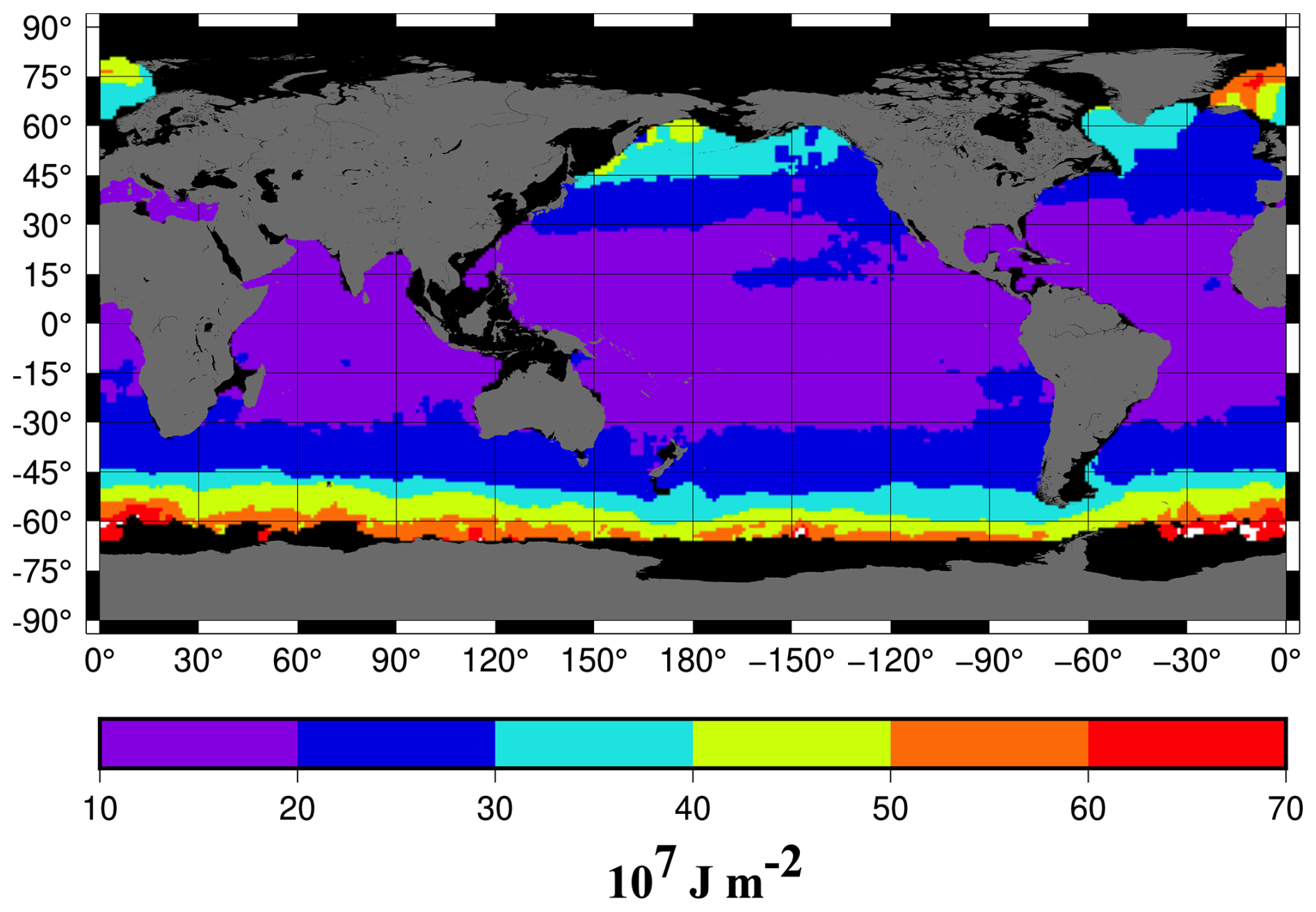
Figure 2 Estimated scale factor to convert satellite SSL grids (in cm) to heat storage anomalies (in 10⁷ J m⁻²).

Finally, we mask the mapped data to remove any estimates in marginal seas or shallow water and above ±65° latitude to be consistent with the SIO no data mask. While we sometimes have sufficient data to find a value in marginal seas, errors are quite large (or are based primarily on the satellite reference) and the OI value mainly depends on observations outside the marginal sea. So, like the SIO product, we choose to ignore them.

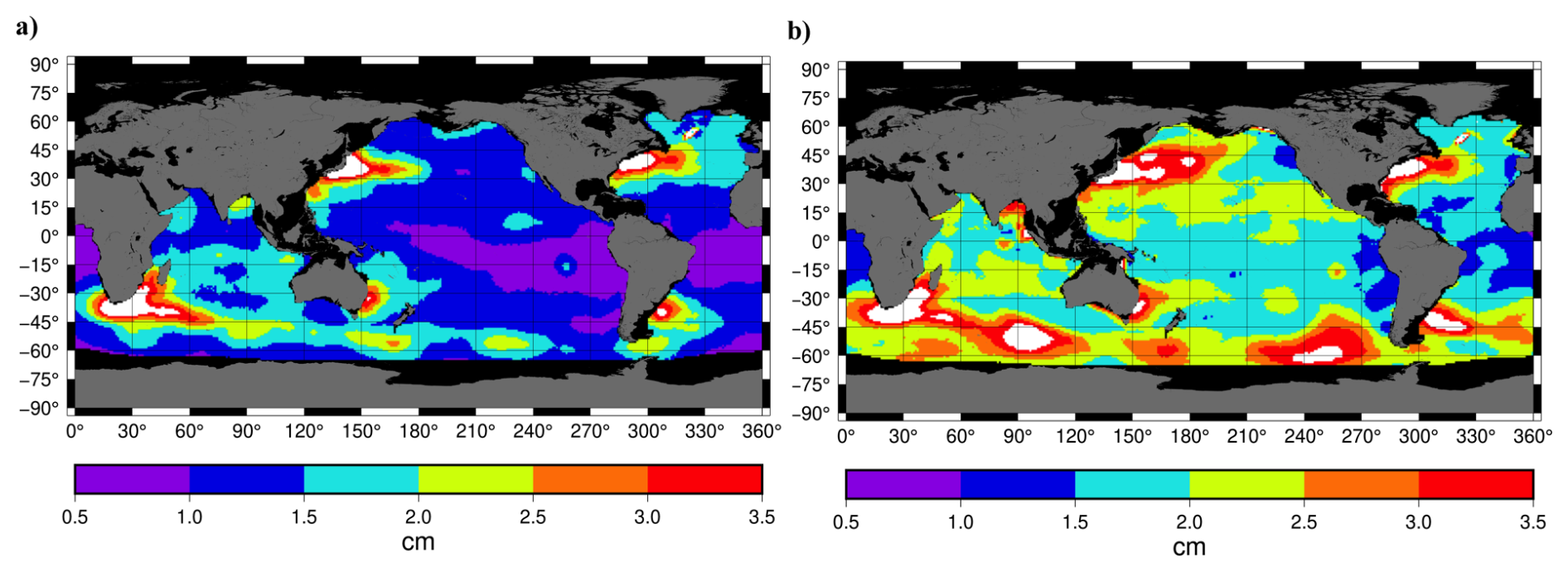
Figure 3 Standard deviation of difference between (a) Argo-only maps and Altimeter-GRACE/FO maps and (b) Altimeter-only maps for January 2010–December 2023. Note that only months that have a GRACE/FO observation are used in the statistics. Values exceeding 3.5 cm are colored white.

3 Analysis of mapped data

To verify that the mapping captures the longwave signal, we calculated the mean autocovariance of all the SSL maps and verified it matches the longwave covariance structure used in the OI mapping (Eq. 7). To demonstrate the relative benefit of using monthly altimetry-GRACE/FO maps as a climatology in the early record, we compare those to maps gridded with only Argo data post 2010 when there is sufficient data to calculate maps with no reference climatology (Fig. 3a). The Argo-only grids are also compared to longwave mapped altimetry grids over the same period (Fig. 3b). It is clear that the altimetry-GRACE/FO maps agree better with Argo-only mapping than only altimetry at most areas outside western boundary currents and the Agulhas Retroreflection, indicating that the altimetry-GRACE/FO maps we utilize as a reference are better for filling gaps in Argo data (especially prior to 2007–2008) over using just altimetry as a reference. This is because GRACE/FO removes large non-steric bottom ocean mass variations in the Southern Ocean and North Pacific (e.g., Jayne et al., 2003) as well as the non-steric global ocean mass variations that are present in altimetry data (e.g., Chambers et al., 2017; Chen et al., 2020). Overall, reduction in error before 2007–2008 where the maps default to the reference is expected to be 2–3 cm in the Southern Ocean and about 1 cm in the rest of the ocean north of 45° S.

We next demonstrate the effect of sampling eddies with limited Argo floats. To do this, we performed a sampling experiment using the altimetry track data. First, the nearest along-track altimetry points in each month to each Argo float location and date are interpolated using bilinear spatial and linear temporal interpolation. These sampled values are then mapped using the two different covariance functions and the standard deviation of the mapped values computed (Fig. 4). Standard deviations of the “eddy-resolution” Argo maps differ from the altimetry maps by over 12 cm in all regions of high mesoscale activity (Fig. 4a) and between 4 and 8 cm in many other ocean regions. This is due solely to the sampling of the Argo floats: i.e., the sampling, even in later years, is insufficient of fully resolving the short-scale (<100 km) variance in the sea level as opposed to the many more altimeter observations. Conversely, differences in the longwave maps peak at about 3–4 cm standard deviation in mesoscale regions, with differences of less than 2 cm over most of the ocean (Fig. 4b). The only exception is in areas with limited Argo floats and these areas are masked in the final products.

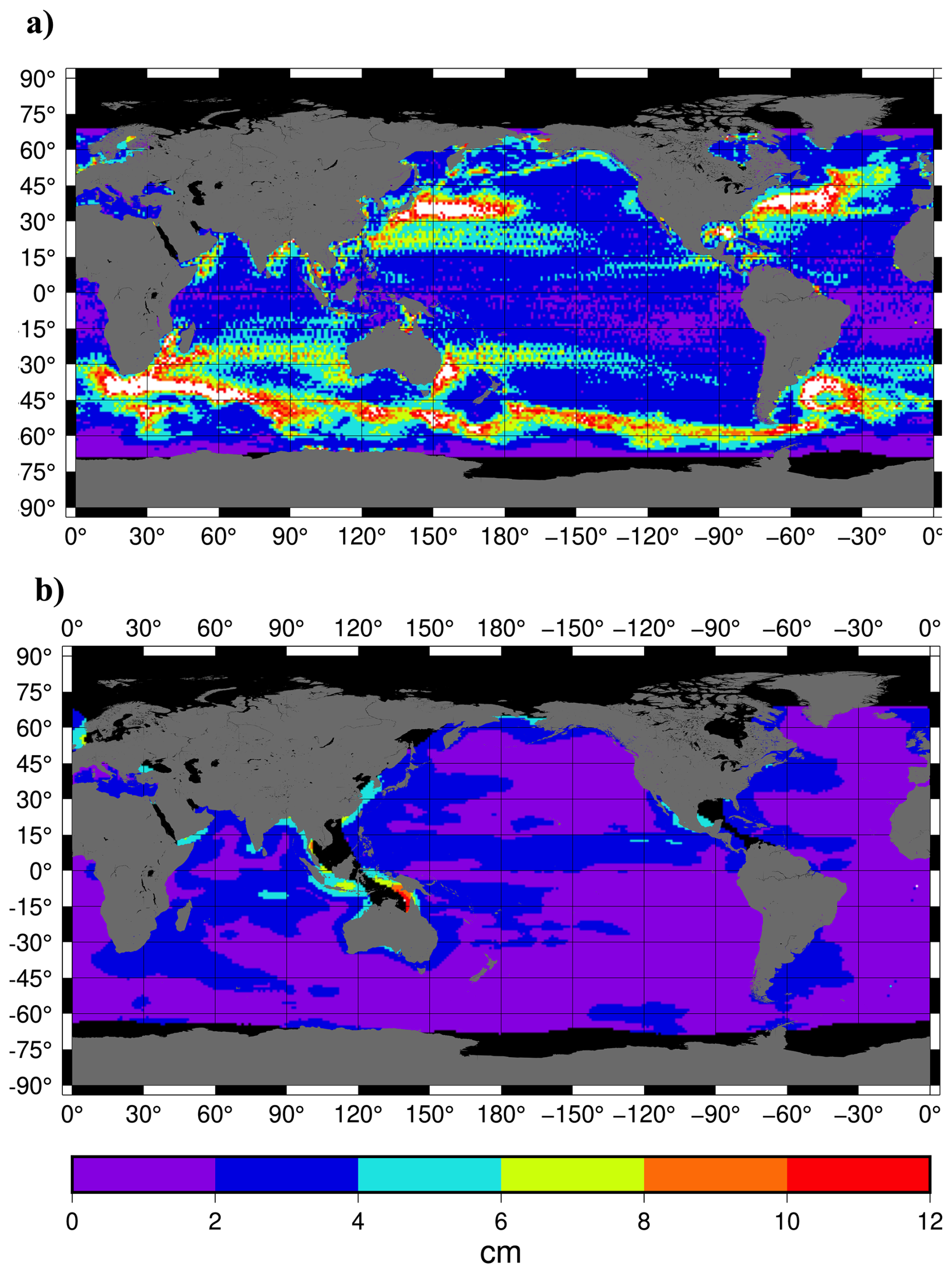
Figure 4 Standard deviation of Argo sampling experiments, where altimetry interpolated to Argo profile locations and times is mapped and compared to maps from the full altimetry. (a) Eddy covariance as modeled as signal (Eq. 7) and (b) eddy covariance as modeled error (Eq. 8), i.e., the longwave mapping.

The sampling error is not perfectly random. To demonstrate this, the sampling error from the experiment (sample – full) is plotted for two grid cells in Fig. 5, one in the Kuroshio extension (150.5° E, 40.5° N) and one in the Agulhas Retroreflection zone (30.5° E, 40.5° S). Biases as large as 20 to 40 cm can persist for upwards of 6 months, resulting in significant non-zero trends (±10 mm yr⁻¹).

The longwave mapping does not significantly alter the global mean sea level estimate (Fig. 6) or basin-scale averages (Table 1), with the trend and annual variations included or if they are removed. Correlations exceed 0.9 (p<0.001) in every case, standard deviations range from 1 mm for the global average to up to 1.5 mm for regional averages. Trend errors range from 0.08 mm yr⁻¹ for the global average, to about as much as 0.2 mm yr⁻¹ over basins. Correlation remains ∼0.99 and standard deviation of residuals are even lower, indicating the long-wave maps capture non-seasonal and long-period variability equally well. We performed an additional test over a smaller area (1500 km by 1500 km) east of Japan where there is significant eddy activity. Correlations remain 0.99 or higher (even after removing a trend and annual variations) and standard deviation of the differences only increases to 2 mm, with trend errors <0.2 mm yr⁻¹. However, if smaller areas are considered (for example 500 km by 500 km in the same area), non-seasonal correlation drops to 0.8 and the standard deviation of differences increases to 4 cm, with significant trend differences (1.7 mm yr⁻¹). Thus, we conclude the longwave mapping is sufficiently accurate to resolve average monthly SSL, TSL, OHC anomalies for the upper 2000 m over areas greater than 1500 km×1500 km. At smaller areas, especially within eddy regions, the longwave maps cannot fully resolve the average and should not be used for studies over regions smaller than this. We would argue the same is true of any Argo-mapped product within eddy regions, even if it includes small-scale variance in the signal covariance function.

Figure 5 Argo sampling error at two regions of high mesoscale eddy activity.

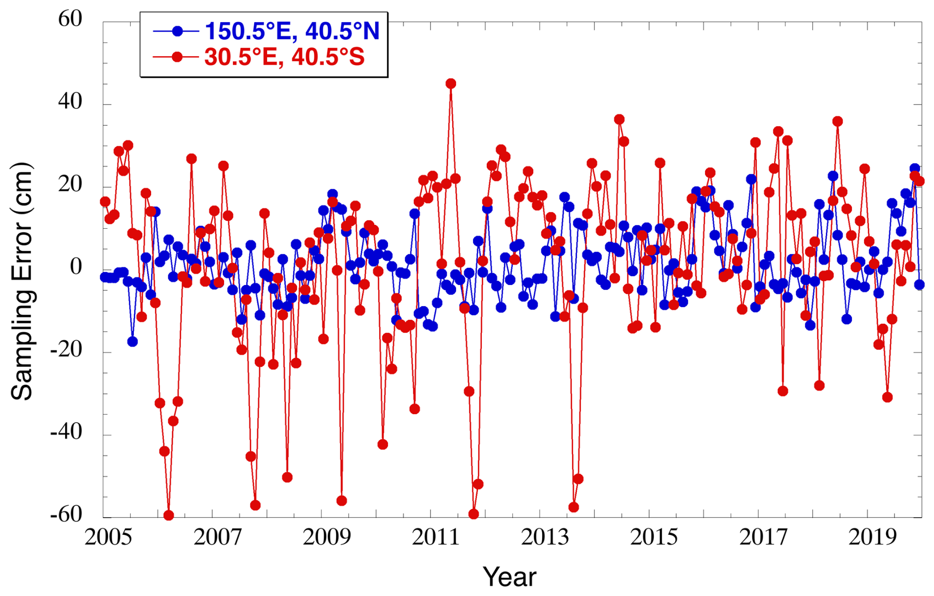
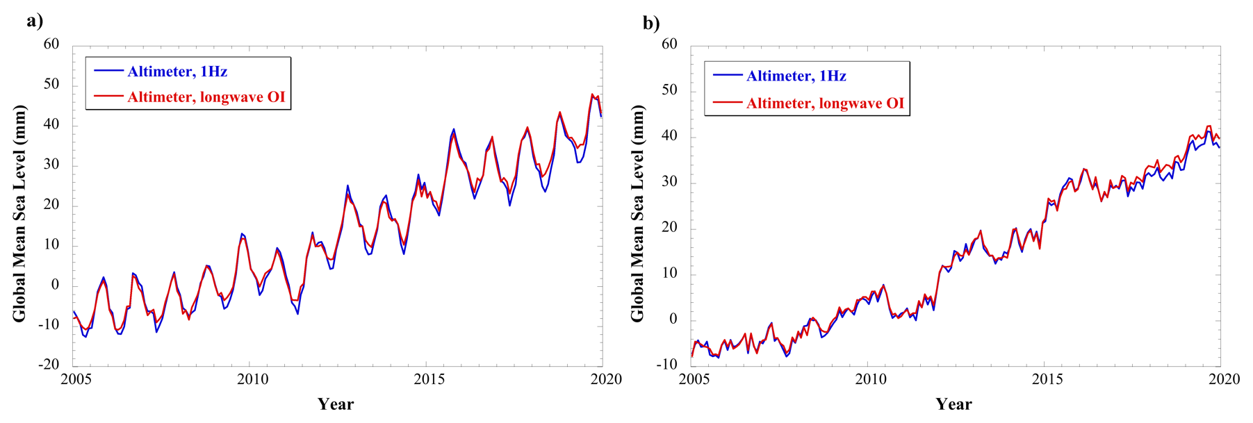
Figure 6 Global mean sea level from raw, 1 Hz altimetry (blue) and from longwave OI maps (red) (a) with annual + semiannual variations and (b) without annual + semiannual variations.

Table 1 Statistics for basin-averages (2005–2019). Difference are eddy OI – longwave OI. North and South partitions are from the equator and the Southern Ocean is defined as all ocean areas south of 30° S.

Figure 7 Global mean steric sea level from reference SSL experiments. (a) With annual + semiannual variations and (b) without annual + semiannual variations. (cyan) No reference, so grids without sufficient Argo profiles for mapping defaults to no data, (blue) a mean monthly climatology based on Argo-only maps from 2008–2018, and (red) the released product, utilizing altimetry-GRACE/FO monthly maps.

The choice of climatology has a noticeable effect on recovered Argo SSL maps in the early part of the record, as others have commented on previously (e.g., Lyman and Johnson, 2008). We have performed three different mapping experiments of Argo SSL to demonstrate this effect on global mean SSL (GMSSL) calculations: (1) using no climatology, so that areas without sufficient Argo profiles are set to no data, (2) using a mean climatology based on Argo mapping only from 2008–2018, and (3) using the monthly satellite estimates (the final product). The results (Fig. 7) show that using no climatology and having gaps in coverage significantly impacts GMSSL until at least 2009, with the largest differences occurring before 2008. Even using a mean climatology to fill gaps creates significant biases (∼5 mm) with the satellite reference before 2007, with smaller (<2 mm) biases up until at least 2011. While it has been previously accepted that Argo data mapped with a climatology reference is sufficient for studying sea level budgets back to 2005 (e.g., Chambers et al., 2017; Blaquez et al., 2018; Chen et al., 2020; Barnoud et al., 2021), this experiment suggests interannual changes in SSL before ∼2008 are sufficiently different from the climatology and that gaps in Argo coverage are still large enough that it can lead to systematic errors in GMSSL. The mean trend from 2005–2024 increases from 1.04 ± 0.04 mm yr⁻¹ for the climatology reference to 1.17 ± 0.04 mm yr⁻¹ using the satellite reference (error at 90 % confidence interval). From 2011 to 2024, when the Argo coverage is more complete and the reference has minimal effect, the trend difference is only 0.08 ± 0.07 mm yr⁻¹ (90 % confidence interval). Trend uncertainty accounts for reduction in degrees of freedom due to non-random residuals as described in Chambers et al. (2017).

As discussed in Sect. 2.3, error maps are provided for each monthly map of SSL, TSL, and OHC anomalies. It should be noted these represent standard errors based on the quantity of data used in the mapping and how well the mapped data represents the expected longwave covariance; they cannot explain the full uncertainty, such as arising from sampling errors (e.g., Fig. 4b) or systematic errors (such as biases or drifts). However, they are useful for seeing where the satellite reference data are used to fill gaps and where the maps are mostly determined by Argo data. Because more data are used in the satellite mapping, the errors are considerably lower than where Argo data is used to update the reference (Fig. 8). Note that in early years (2003–2005 especially), the standard errors often have a “bullseye” pattern, with lower errors in the center and higher values increasing with radius (see 2003 and 2005 in Fig. 8). This reflects lower errors near a cluster of Argo floats, and larger errors on grids that are within the radius of the OI mapping but with no (or few) Argo floats in them during that month. Oftentimes, there is an abrupt transition from high errors to low errors where there are no Argo floats and so the mapping defaults to the satellite reference.

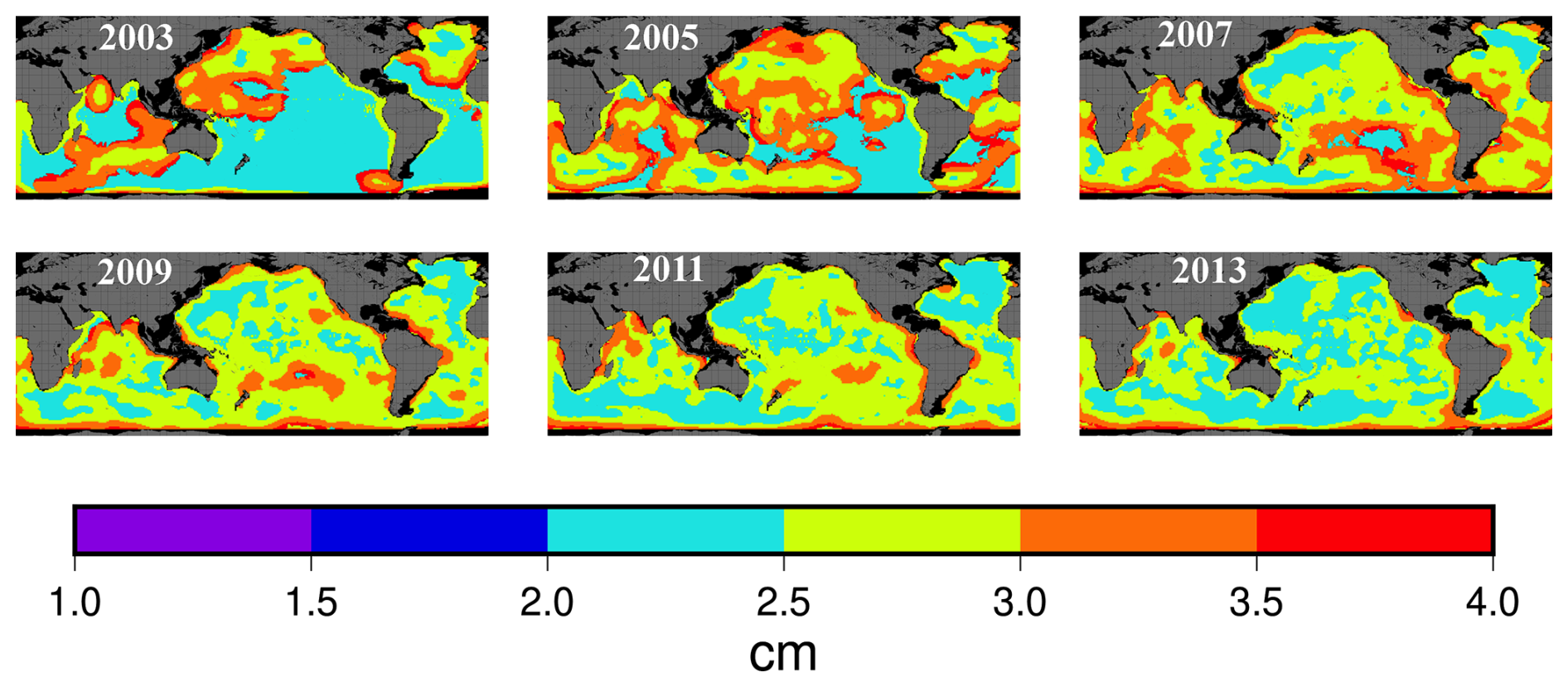
Figure 8 Standard error for SSL in June for years indicated.

Figure 9 Global mean steric sea level from altimetry-GRACE (gray), USF mapped SSL (red), and SIO mapped $T/S$ grids (blue), (a) with annual + semiannual variations and (b) without annual + semiannual variations.

The satellite data tend to dominate the mapping from 2003 to 2005 but are still the primary source in some areas of the South Pacific as late as 2008 and 2009 (Fig. 8; see also Figs. S1 and S2). This should result in an improved estimate of SSL, TSL, and OHC in these areas over using a mean monthly climatology if there are significant interannual fluctuations there – e.g., El Niño/La Niño signals in the eastern Pacific, which did not have complete Argo coverage in every month until 2008 (Fig. S1). By 2010, most of the ocean has sufficient Argo coverage each month that maps are computed fully from Argo data and the reference does not matter, so the error maps reflect the Argo mapping error. TSL errors from the satellite data are identical to the SSL errors from satellites (as the same satellite reference maps were used for both TSL and SSL), but the Argo errors differ, since TSL is directly computed from Argo profiles. OHC errors are merely the TSL errors scaled to the appropriate units.

It is beyond the scope of this manuscript to compare our results to every gridded Argo product available. However, we do compare the global mean steric (Fig. 9) and thermosteric sea level (Fig. 10) computed from our product (designated USF for University of South Florida) with that computed from the SIO gridded $T/S$ data. The SIO product has been shown to have smaller salinity errors than other available products (Blaquez et al., 2018; Barnoud et al., 2021; Liu et al., 2023). Thus, the comparison provides some insight into how our processing may inform sea level budget studies. We also show a global SSL series computed by differencing the altimetry track data (from Beckley et al., 2022) and GRACE/FO (from the JPL Release RL06Mv02 mascons) – the same data used for the longwave gridded reference grids – but here we do no additional mapping, just perform a global area-weighted average of the original resolution data. Several minor corrections are applied to remove signals that the Argo data do not observe (see Blaquez et al., 2018, for why these are necessary): (1) a correction for glacial isostatic adjustment is added to the altimetry (Nerem et al., 2010; value used =0.3 mm yr⁻¹), (2) a correction for Jason-3 radiometer drift is added to the Jason-3 altimetry as the product we used did not include this at the time of processing (Brown et al., 2023), and (3) an estimate of the mean global steric sea level rate below 2000 m (0.11 mm yr⁻¹) from Purkey and Johnson (2010) was removed to align with the 2000 m max depth used in the Argo profiles. Note that after 2010, the altimeter-GRACE/FO time series is nearly independent, as there are sufficient Argo profiles that a reference is not needed (Fig. 7).

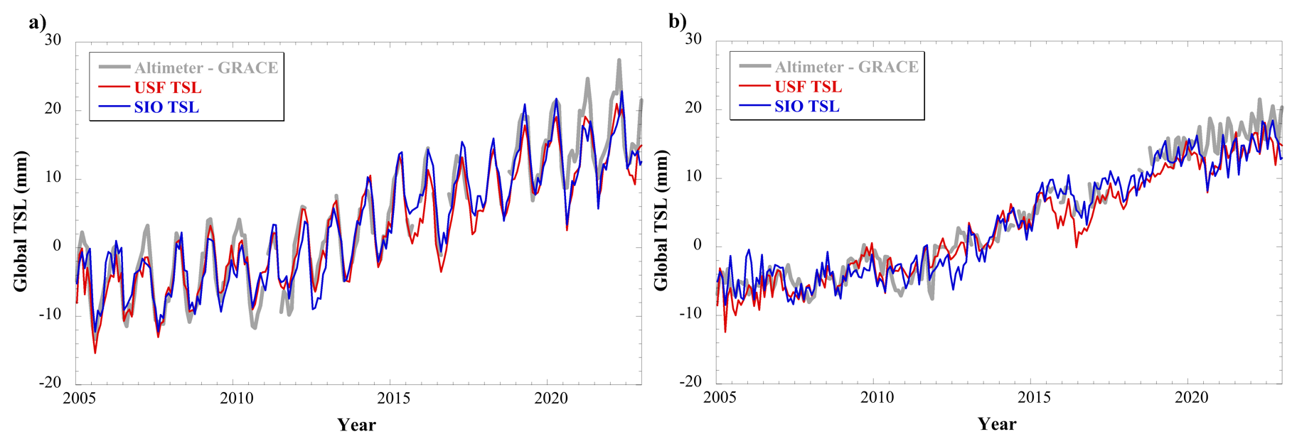
Figure 10 Global mean steric sea level from altimetry-GRACE (gray), and thermosteric from USF (red), and SIO (blue), (a) with annual + semiannual variations and (b) without annual + semiannual variations.

As noted in multiple studies (Blaquez et al., 2018; Chen et al., 2020; Barnoud et al., 2021), there is a significant misclosure between the satellite estimate and the Argo GSSL estimate after 2019–2020 for both the SIO and USF products (Fig. 9). The SIO estimate matches altimetry well in 2019 and the first half of 2020, but then falls off rapidly, while the USF estimate is significantly lower starting in 2018. However, the USF and SIO estimates generally agree after 2020.5, both being significantly lower than the satellite estimate.

From this analysis, we conclude that GSSL computed from our long-wave steric sea level maps is in general agreement with that derived from the currently available SIO $T/S$ maps, except for two notable occasions: in 2015 and between 2018–2020.5. The difference in 2015 is interesting, as the USF estimate agrees better with the satellite estimate for part of the seasonal variation (closer at the trough than at the peak. Moreover, when global thermosteric sea level (GTSL) is compared instead (Fig. 10), there is no change in behavior during 2015, but USF and SIO GTSL agree well for all other periods. This suggests that the difference between USF and SIO GSSL in 2018–2020.5 is due to unresolved salinity errors that are not flagged (and so get into the USF processing) but that SIO has edited out. Unfortunately, there is no documentation that we can find on recent SIO processing standards that can explain how this was accomplished. Moreover, the SIO and USF GSSL curves both depart significantly from the altimetry-GRACE curve after 2020, whereas the SIO and USF TSL curves differ by a smaller amount. This further suggests unresolved salinity errors in a large number of profiles after 2018, even though we have utilized a release of Argo $T/S$ profiles that has added new flags and adjustments to identify such problem floats (Wong et al., 2023). We removed such flagged/adjusted floats from our processing stream (see Sect. 2.1). However, this does not prevent large and unrealistic global halosteric signals post 2018, so we must conclude that unidentified salinity errors remain in enough profiles to affect the global halosteric signal.

However, the differences in 2015 can't be explained by salinity errors, as they appear in both the USF GSSL and GTSL curves. We experimented with an additional 3-sigma editing of the $T/S$ profiles (based on difference with the climatological profiles); while that removed a small number of profiles, it did not significantly affect the recovered maps in those periods, or GSSL/TSSL. Because of this, we selected not to use a 3-sigma editing

Unfortunately, because the exact retained floats and profiles used in the SIO mapping are not provided, we cannot test if our analysis would change if we used the same profiles in our mapping. We suggest it would be beneficial for all Argo data centers producing statistically mapped data to provide a list of the exact float numbers and profile dates used in their analysis so that mapping experiments with the same raw data can be conducted by other groups. For this reason, we distribute the float numbers and dates that we utilize in our mapping.

A common use of OHC anomalies for the upper 2000 m is to take the time-derivative of the global average (in W m⁻²) and use this in computing the global ocean heat uptake (OHU) (e.g., Hakuba et al., 2021, 2024; Loeb et al., 2021; Lyman and Johnson, 2023). The upper ocean above 2000 m explains approximately 90 % of the OHU, while the ocean deeper than 2000 m explains the remainder (Purkey and Johnson, 2010; Hakuba et al., 2021). Importantly, interannual to decadal-scale changes in OHU are dominated by the changes above 2000 m. Typically upper ocean OHC derivatives are combined with an estimate of deep warming below 2000 m (assuming a steady gain of heat), using values determined from deep and repeat hydrographic sections (e.g., Purkey and Johnson, 2010; Johnson and Purkey, 2024). The value commonly added is 0.06 ± 0.04 W m⁻² (e.g., Hakuba et al., 2024). Additionally, the OHC derivatives are often normalized by Earth's surface area at the top of the atmosphere (5.14×10¹⁴ m² at 20 km above the Earth's surface) and not the ocean area, to bring it into line with satellite measurements of Earth's Energy Imbalance (EEI) (e.g., Hakuba et al., 2021; Loeb et al., 2021).

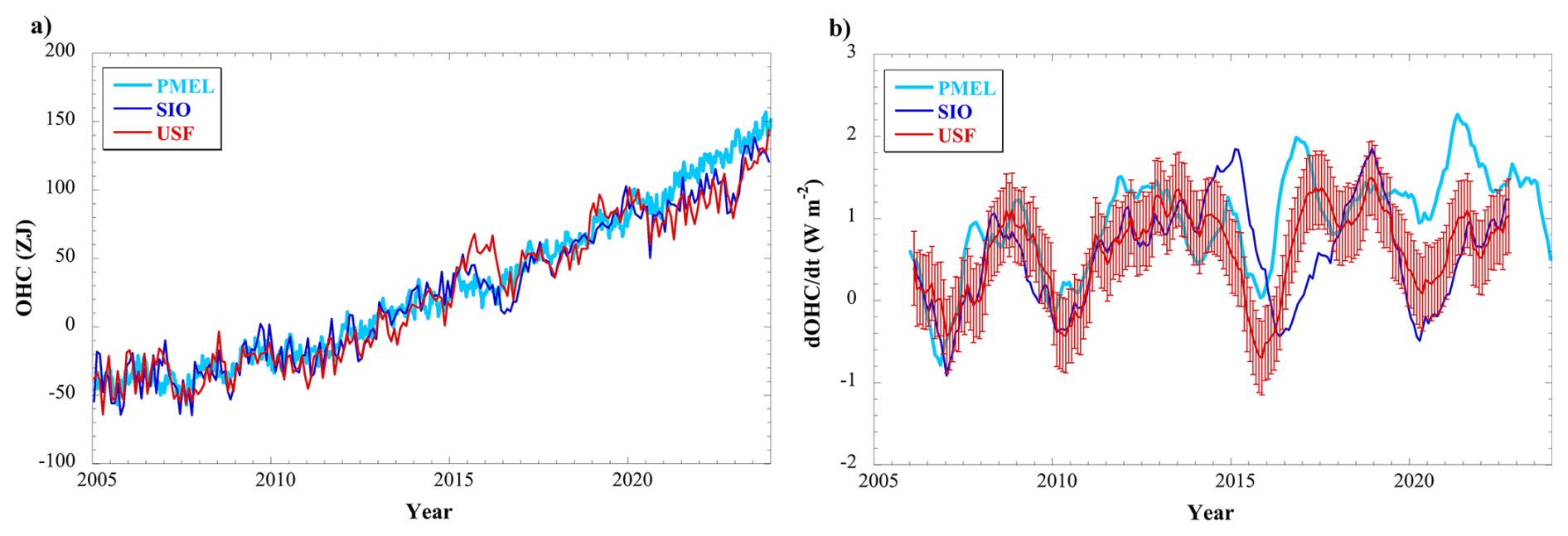
Figure 11 (a) Global OHC anomalies above 2000 m, after removing mean annual/semiannual sinusoids. Data shown are from (cyan) the Random Forest Regression Ocean Maps at the NOAA Pacific Marine Environmental Laboratory (PMEL; Lyman and Johnson, 2023, 2025; https://www.pmel.noaa.gov/rfrom/, last access: 7 November 2025), (blue) the SIO $T/S$ grids (blue), and (red) the USF OHC anomaly grids. (b) Two-year running trends computed from (a) which reflects $\mathrm{d}\text{OHC}/\mathrm{d}t$ for the upper 2000 m over time. Uncertainty is the 90 % confidence interval based on least squares fit, and accounts for reduction serial correlation in residuals as described by Chambers et al. (2017). Uncertainty is only shown for the USF calculation, but the SIO and PMEL uncertainty is similar in magnitude. The PMEL data were referenced to the mean of 2008–2016 to be consistent with the mean of the USF grids. One ZJ=10²¹ J.

Here, we compare the global OHC anomalies above 2000 m computed from our OHC grids with those from computed from the SIO $T/S$ grids as well as those computed by Lyman and Johnson (2023), which use altimetry and satellite sea surface temperature measurements as a reference before combining with Argo (Fig. 11a). Before 2015, the three datasets agree well, showing similar overall trends and interannual variability. While the Lyman and Johnson (2023) grids are specifically formulated to resolve eddy signals, it is clear this has little effect on the global average and that the longwave mapping we use is sufficient. within estimated errors, except for the periods that include 2015 (Fig. 11). During 2015 to early 2016, there is disagreement as noted previously (e.g., Figs. 9 and 10 and associated discussion). The USF OHC appears to be the outlier in 2015, but by early 2016, it agrees with the PMEL OHC, whereas the SIO OHC has a significant drop throughout 2016 until 2017. This further supports the idea that there may be unresolved issues with Argo temperatures in some floats in 2015 and 2016 that warrants further investigation.

After 2020, there is a significant change in behavior between the USF/SIO OHC curves and that from the Lyman and Johnson (2023) analysis. The PMEL analysis shows a steady rise in OHC after 2020, whereas USF and SIO grids indicate more interannual variability, with a drop from 2020–2021, followed by a subsequent rise. It is interesting that the PMEL curve follows the general trend in satellite altimetry over this time (e.g., Fig. 10), which suggests that the global OHC from the PMEL analysis may be more dependent on the altimetry reference than our analysis, as we find little to no impact of different references in the global average (Fig. 7). Notably, the USF curve post-2020 follows that of SIO, which uses only Argo data (and an Argo-based climatology) in the mapping.

These subtle differences in OHC are reflected in the time-derivative (Fig. 11b), which we calculated using running 2 year trends (along with annual and semiannual sinusoids) from the global average OHC (and converting $\mathrm{J}{\mathrm{m}}^{-\mathrm{2}}{\mathrm{yr}}^{-\mathrm{1}}$ to W m⁻²) – the time stamp used is the middle of each 2 year window and a one-month step was used. Values agree reasonably well before 2020 (noting the small differences in 2015–2017 noted earlier). The mean values for 2005 to 2023 are similar for USF and SIO (USF: 0.58 ± 0.18 W m⁻²; SIO: 0.54 ± 0.21 W m⁻²) but are significantly higher for the PMEL OHC derivative (0.96 ± 0.19 W m⁻²). This is primarily caused by higher values post 2020. In the first half or of the record (2005–2015), the mean PMEL values of $\mathrm{d}\text{OHC}/\mathrm{d}t$ are 0.63 W ± 0.24 W m⁻², whereas in the second half (2015–2024), the mean of the PMEL series is 1.36 ± 0.20 W m⁻².

4 Data availability

All data utilized in this project is publicly available. GRACE data can be downloaded from https://doi.org/10.5067/TEMSC-3JC62 (Wiese et al., 2019). Altimetry data can be downloaded from https://doi.org/10.5067/ALTTS-TJA51 (Beckley et al., 2022). Argo data were collected and made freely available by the International Argo Program and the national programs that contribute to it and can be downloaded from https://doi.org/10.17882/42182 (Argo, 2000). The Argo Program is part of the Global Ocean Observing System. The OHC anomalies from the NOAA Pacific Marine Environmental Laboratory Random Forest product can be downloaded from https://www.pmel.noaa.gov/rfrom/ (last access: 7 November 2025) (Lyman and Johnson, 2025). The final mapped SSL, TSL, and OHC maps (and error maps) are available at from https://doi.org/10.17632/dsjkkhvywr.1 (Chambers and Reinelt, 2025).

5 Conclusions

We have described a new set of steric and thermosteric sea level anomaly gridded data, at monthly resolution between 2003 and 2023. Additionally, ocean heat content anomalies are also available. Maps are based on using a satellite estimate (altimetry – GRACE/FO) as a starting guess, then updating with values derived from Argo profiles. The data have been intentionally mapped to retain only the longwave portion of the covariance, to reduce sampling errors from limited Argo observations in regions of high mesoscale activity; limited Argo profiles (especially from floats within an eddy) may lead to biased estimates in individual grid cells if the short variance signal is mapped. As we have demonstrated, there is no significant difference between the longwave or shortwave mapped data when averaged over ocean basins and globally.

These data complement mapped data from other sources (e.g., SIO, the Chinese Second Institute of Oceanography, EN4.2.1 the Meteorological Research Institute of Japan, JAMSTEC), but provide useful benefits for scientists working on sea level budget and ocean heat uptake studies:

1. Data are provided in integrated values necessary for these studies, not in $T/S$ at depth that require conversion and integration.

2. The monthly satellite reference likely improves estimates during 2003 to ∼2008 when Argo sampling still has substantial gaps (e.g., Figs. 3 and 7).

3. Error maps are provided for SSL, TSL, and OHC for each month. Such error maps are not routinely provided by other processing centers.

4. The integrated SSL, TSL, halosteric sea level, and OHC anomalies for each float profile that met the flagging and editing criteria is also distributed. This allows users to see the locations and time of the exact floats used in the analysis, which may be of use for understanding differences between other data center mapping strategies (e.g., the difference between our grids and those of SIO in 2015). Again, this information is not available from other centers that we have been able to find.

There are limitations to the data. These maps are intended to represent SSL, TSL, and OHC for the upper 2000 m of the ocean. They do not account for any steric variations below 2000 m. However, this is true of any Argo-based mapped product of $T/S$ or OHC above 2000 m. New data from the deep Argo array indicate the possibility of relatively large steric anomalies below 2000 m in at least one small area of the tropical Atlantic (Zilberman et al., 2025), but complete knowledge of deep steric signals is still very much an open research area. The maps we have produced will be as useful as any other current Argo-based product for global and basin-scale sea level and heat budgets that are available at the present, provided the studies are for areas larger than about 1000 km by 1000 km. Because our data are mapped over long wavelengths, they will not capture small-scale variations in sea level or OHC. While this was done to improve the recovery of unbiased values of the background state in areas of high mesoscale activity, it will also reduce signal in other areas, such as in the tropics where there can be signals from shifts in the zonal equatorial currents. They likely will also underestimate El Niño variations in the eastern and western Pacific. Users focusing on these specific regions should take this under consideration.