Ground-based atmospheric measurements at the Onsala Space Observatory (Sweden): data & trends (2009–2025)

This study presents a comprehensive long-term dataset of ground-based atmospheric observations collected at the Onsala Space Observatory (OSO), Sweden, between August 2009 and April 2025 (https://doi.org/10.1594/PANGAEA.984087, Mascaut et al., 2026a; https://doi.org/10.1594/PANGAEA.984085, Mascaut et al., 2026b). The dataset includes measurements of temperature, relative humidity, atmospheric pressure, precipitation, wind speed, gust and direction, and solar irradiance. It offers high-resolution insight into local weather patterns and seasonal variations, making it a valuable resource for climate monitoring and regional environmental studies. Preliminary analysis reveals a warming trend of ∼ 0.15 °C yr⁻¹, with significant seasonal contrasts: the most pronounced increase occurs in winter (203.3 % above the annual trend, so winters are becoming milder), followed by autumn (80.1 %), spring (62.3 %), and summer (32.9 %). Rain rate trends show a significant decrease over the study period. Anomalies such as the particularly cold winters in 2009–2010 and 2010–2011 or the particularly warm winter in 2019–2020 are highlighted and linked with the North Atlantic Oscillation (NAO) phases. This dataset complements existing data for local trend analysis and atmospheric modeling in northern Europe.

1 Introduction

In recent years, the scientific community has increasingly recognized the value of long-term, high-quality ground-based measurements to capture the nuances of surface processes and atmospheric interactions. Such datasets not only support the development and refinement of geophysical models but also enhance the reproducibility and consistency of climate research.

Understanding local expressions of climate variability further depends on sustained, high-resolution (e.g. 1 min resolution) observations of key atmospheric parameters. In situ ground-based measurements, with their ability to capture local-scale processes, diurnal cycles, and extreme events at high temporal resolution, offer critical insights that complement satellite and reanalysis datasets (Ménard et al., 2019). While extensive observational networks exist across Northern Europe, high-frequency, multi-variable datasets covering more than a decade are still relatively uncommon - especially in coastal and maritime regions, where climate variability is strongly modulated by the interaction of oceanic and continental air masses.

The Onsala Space Observatory (OSO), situated on Sweden’s west coast, provides a valuable multi-year record of key near-surface atmospheric parameters. These include air temperature, relative humidity, atmospheric pressure, wind (speed, gusts, direction), precipitation (rate and accumulations), and solar irradiance. Each of these variables plays a central role in the energy and water cycles of the atmosphere and is directly relevant to climate monitoring. For example, temperature and humidity are fundamental indicators of thermodynamic state and climate change (Douville et al., 2021); wind patterns influence regional heat and moisture transport (Donat et al., 2010); precipitation and its intensity determine hydrological extremes and flood risks (Trenberth, 2011); solar irradiance governs surface energy balance and is critical for both climate models and renewable energy assessments (Wild et al., 2015); and atmospheric pressure provides insight into synoptic-scale circulation patterns.

This descriptive paper does not aim to introduce novel findings but rather to provide valuable data and offer an overview of the potential insights that such a dataset can yield. Although the measurements presented are local, the analysis demonstrates their relevance and potential utility for more advanced atmospheric or climate research conducted at broader spatial and temporal scales. In the present paper, the context in which the measurements were taken, as well as a brief presentation of the dataset and the instruments, are provided in Sect. 2. An initial analysis (time series and seasonal behaviour) of this dataset is presented in Sect. 3. Finally, Sect. 4 shows the inter-annual trends of the various measured parameters, and the first conclusions are presented in Sect. 6.

2 Study area and instrumentation

2.1 Study area – The Onsala Space observatory (OSO)

The Onsala Space Observatory (OSO), located 45 km south of Gothenburg in western Sweden, operates multiple geodetic and geophysical facilities since 1979, including Very Long Baseline Interferometry radio telescopes, a superconducting gravimeter, Global Navigation Satellite System stations, tide gauges, and many others (e.g. Haas et al., 2023; Varenius et al., 2021; Scherneck et al., 2020; Ning and Elgered, 2025). An overview of the observatory with the instrument locations is depicted in Fig. 1. Instruments used in this study are highlighted in red. The OSO has a strategic location on the west coast of southern Sweden at the land/sea interface. Land coverage is characterized by grassland, forest and sea (see photos in Fig. 1).

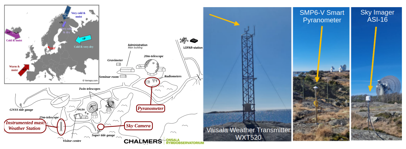
Figure 1 Locations and geographical context of the different measurements made at the OSO. Top left: Large-scale map (source: https://vemaps.com, last access: 17 June 2025) and main air masses. Center: OSO map with instrument locations (atmospheric sensors highlighted in red). Right: Photos of each instrument used (Vaisala Weather transmitter WXT520, SMP6-V Smart Pyranometer and Sky Imager ASI-16).

The OSO atmospheric measurements are influenced by both local and large-scale phenomena. Indeed, Lepy and Pasanen (2017) show that the position of Northern Europe between the ocean and the continent and between the tropical and polar regions favours the confluence of multiple air masses (Fig. 1 top left, adapted from Lepy and Pasanen, 2017). Thus, the OSO is a meeting place for the maritime Polar (mP) air masses, the maritime Tropical (mT) air masses, the continental Polar (cP) air masses; the maritime Arctic (mA) air masses responsible for the coldness from February to the arrival of the spring; and the continental Arctic (cA) air masses starting in the autumn. In this map, we can thus see that, depending on the seasons and atmospheric movements, Sweden can be subject to different regimes/air masses. Each of the later has specific thermodynamic properties: they can be warm or cold, bring humidity or, on the contrary, dry out the atmospheric layers. For example, the maritime Polar air masses bring cold and moist air from south of Greenland, and the maritime Tropical air masses imply warm and moist air that is important for the energy transfer from the warm Atlantic waters to Northern Europe. Sweden, and in our specific case the OSO, is at the crossroads of these air masses.

Large‐scale pressure patterns such as the North Atlantic Oscillation (NAO) further modulate our region’s winter climate. During boreal winter (November–April), the NAO manifests as a north–south dipole between the Azores High and the Icelandic Low. Appendix A shows the monthly NAO indices (Fig. A1) as well as the impact of the NAO phases on the Swedish West coast weather conditions, depending on the seasons (Table A1). In its positive phase, strengthened westerlies channel mild, moist air into northern Europe, yielding warmer, wetter winters, whereas its negative phase weakens the westerly flow, resulting in colder, drier conditions across the region (Iles and Hegerl, 2017; Hurrell, 1995; Hurrell and Loon, 1997; Deser et al., 2017). These insights are compared with ground-based measurements conducted at OSO, throughout this paper.

In addition, the site is situated far away from major sources of air pollutants, and the measurements are performed in background air most of the time (≃ 60 %, Wängberg et al., 2016).

2.2 Instrumentation

The current section gives a description of the sensors deployed and the quantities measured (see Table 1).

Table 1 Sensors of the ground-based atmospheric measurements at the OSO. The height of each instrument is given in meters above the sea level (m a.s.l.). Specified accuracies and measuring ranges are manufacturer information. The corresponding data links are also given.

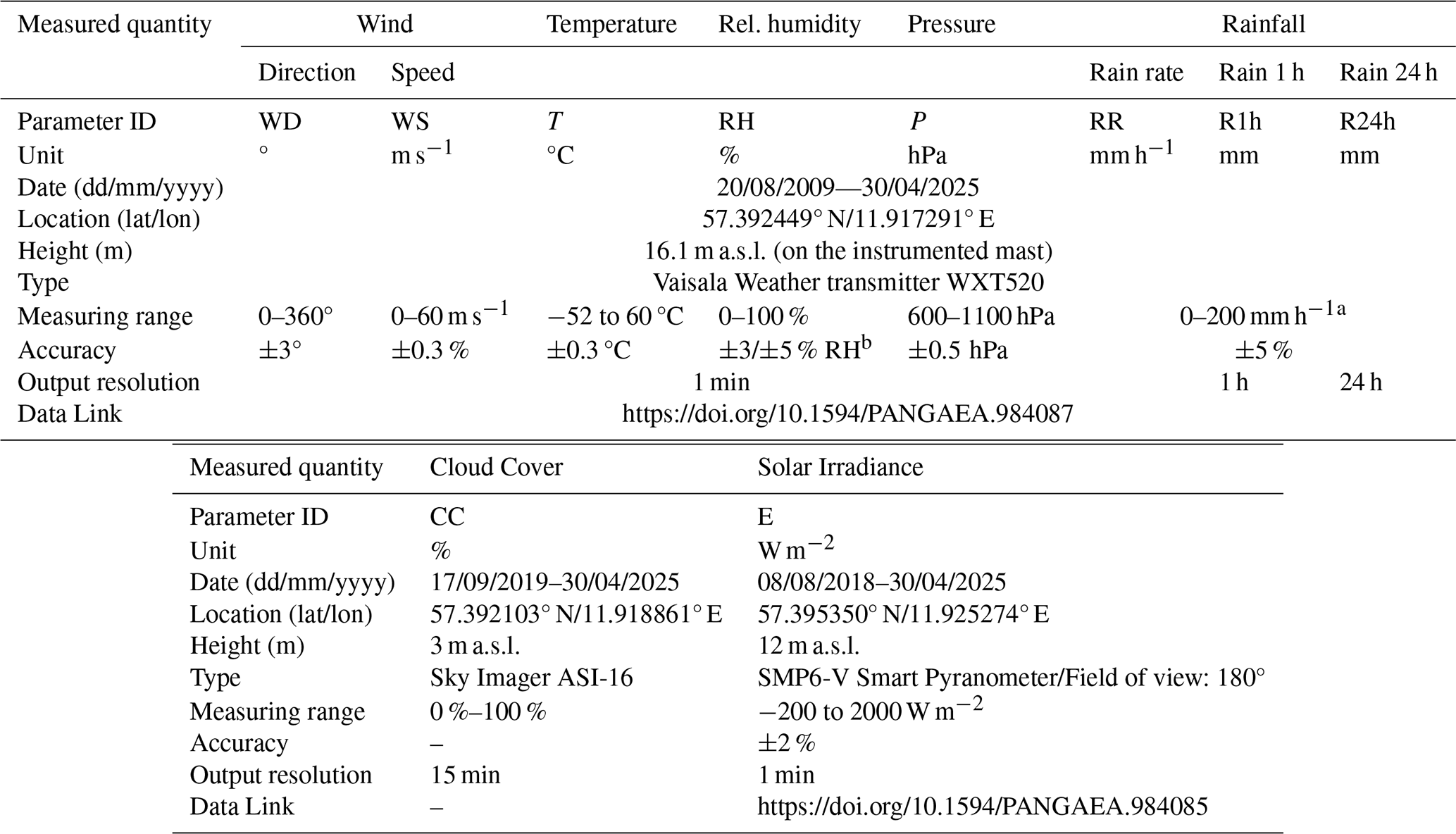
^a broader range with reduced accuracy; ^b ±3 % RH at 0 %–90 % RH and ±5 % RH for 90 %–100 % RH

2.2.1 Vaisala Weather station on the instrumented mast

The Vaisala weather transmitter WXT520 is an integrated instrument that combines multiple sensors to measure thermodynamic and meteorological parameters (including temperature, humidity, pressure, precipitation, and wind) at a single location and at a 1 min sampling frequency. The corresponding sensors are mounted at the top of the tower at ∼ 16 m a.s.l. (Table 1). Data are continuously acquired, and 1 min averages are recorded. The resulting dataset covers the period from August 2009 to April 2025 (included).

The Vaisala wind sensor, located on the same mast, captures real-time data on wind speed, gust and direction. Wind measurements are based on an ultrasonic sensor (WINDCAP^®) that determines speed and direction from the transit time differences of ultrasonic pulses between multiple transducers. Wind speed and direction are provided at a temporal resolution of 1 min and represent mean values over this time. Wind gust is defined as the maximum wind speed observed over a 3 s internal interval within each reporting period. As before, the wind sensor is measuring continuously between 2009 and 2025.

The rain sensor is a device that accurately measures real-time rain rate (RR: rain intensity in mm h⁻¹), and cumulative rainfall over 1 h (R1h in mm) and 24 h (R24h in mm) periods. Precipitation measurements from the Vaisala WXT520 utilize an acoustic impact sensor (RAINCAP^®) that estimates rainfall intensity from the characteristics of raindrop impacts. The rain rate (RR) is provided at a 1 min temporal resolution and expressed in mm h⁻¹. Hourly and daily accumulations (the latter defined using the 06:00–06:00 local time convention) are calculated by summing the 1 min precipitation amounts derived from the rain rate over the corresponding periods. The measurement dates are the same as for the other sensors.

2.2.2 Sky camera

The sky camera imager is an optical instrument designed to capture high-resolution, real-time images of the sky. This camera is intended to be used for capturing all-sky images in the visible spectrum, inspection, and analysis of clouds during daytime with a 180° field of view to the sky and the horizon. Here, we estimate the cloud cover (cc) values by counting the clear and cloudy pixels in the images and calculating cc $=\mathrm{100}\times$ number of cloudy pixels/total number of pixels. Cloudy and clear pixels are identified using the FindCloudsTrinity (FCT, Schreder/CMS) software applied to images from the ASI-16 sky imager. The classification is based on the Blue/Red and Blue/Green (BRBG) color ratios derived from the RGB image channels, which allow for discrimination between clouds, haze, and clear sky. Pixels are classified using the BRBG-based cloud index, resulting in a binary cloud mask from which the cloud cover is computed as the fraction of cloudy pixels. This approach has been widely used and validated in previous studies for cloud and irradiance analysis (e.g. Song et al., 2023; Nevins and Apell, 2021; Long et al., 2006; Sabburg and Long, 2004), and further implementation details are available in the instrument manuals (Schreder CMS, 2025b, a). The sky camera records images every 15 min between September 2019 and April 2025. Note that no images were saved between 30 June (12:00) and 5 August (12:00) 2022.

2.2.3 Pyranometer

As an addition to the previous instruments (the Vaisala Weather transmitter WXT520 and the Sky Imager ASI-16), global radiation is measured using a pyranometer, SMP6-V Smart Pyranometer (Kipp & Zonen). The sensor is installed 12 m a.s.l. (see OSO map on Fig. 1 for location). It measures the global horizontal solar irradiance over a wide temperature range (−40 to +80 °C) with a 180° field of view. The data are updated every minute, from August 2018 to April 2025. To match the data from the sky camera, we use here the observations between September 2019 and April 2025. The year 2022 exhibits a disruption in continuous measurements over a certain period due to a sensor malfunction.

3 Data at the OSO (2009–2025)

The data presented here reflects the evolution of ground-based atmospheric parameters measured at the OSO over a period of 15 years and 8 months (August 2009–April 2025). For the presentation of this dataset, we have structured the measurements as follows: the temperature, relative humidity and pressure sensors (Sect. 3.1, 3.2 and 3.3), the rain sensor (Sect. 3.4), the wind sensor (Sect. 3.5), and the combination of computations derived from the sky camera and the pyranometer (Sect. 3.6).

Figure 2 (left side) displays: (a) temperature and relative humidity measurements at 1 min resolution for the entire period (2009–2025); (b) monthly averages of these measurements (derived from panel a); (c) atmospheric pressure measurements at 1 min resolution (at ∼ 16 m a.s.l.) along with their monthly averages; and finally, (d) and (e) monthly averages of temperature and relative humidity, respectively, for each year. Note that the averages for 2009 and 2025 should be interpreted with caution since the data do not cover complete years.

It has been shown in numerous studies that weather parameters are affected in various ways and by processes of different scales (e.g. Busuioc et al., 2001; Rimbu et al., 2001). The atmospheric processes impacting meteorological parameters vary not only by region, but also between seasons (e.g. Dankers and Hiederer, 2008; IPCC, 2022). Therefore, our analysis takes seasonal variations into account.

On the right side of Fig. 2, the daily anomalies (cycles) for the three parameters (T, RH and P) are presented according to season. For this purpose, the seasons are defined as follows: (a) winter: 1 December to 28 February (or 29); (b) spring: 1 March to 30 May; (c) summer: 1 June to 31 August; and (d) autumn: 1 September to 30 November. Thus, the data are binned by season, and the daily mean value is subtracted, so the resulting anomaly represents the deviation from this reference value (i.e. the diurnal variations). Data from 2009 and 2025 have been excluded from this calculation.

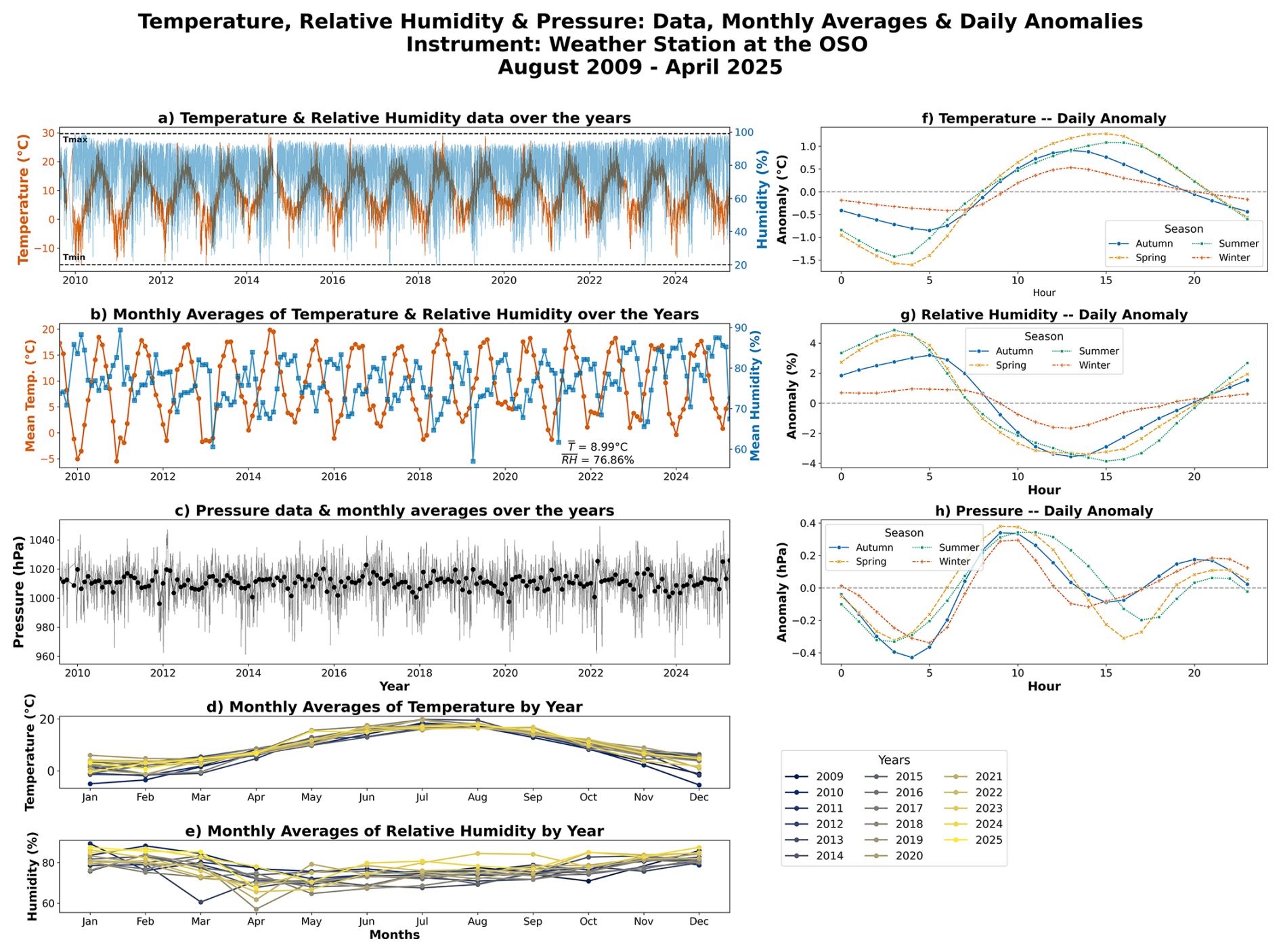
Figure 2 Temperature, relative humidity, and atmospheric pressure recorded at ∼ 16 m a.s.l. by the Vaisala Weather transmitter WXT520 at the OSO over a 15-year and 8-month period. (a) Time series (1 min temporal resolution) of temperature (°C, red) and relative humidity (%, blue) data. (b) Monthly mean values (derived from a) of temperature and relative humidity, with overall means. (c) Time series of atmospheric pressure (hPa, grey) at ∼ 16 m a.s.l., at 1 min resolution, including monthly means (black). (d) Monthly mean temperature by year, color-coded by calendar year. (e) Monthly mean relative humidity by year, color-coded by calendar year. (f–h) Diurnal anomalies (from daily mean) of temperature (f), relative humidity (g), and pressure (h) averaged by season.

3.1 Dynamics of Temperature

The seasonal cycle of temperature is well-defined: (1) cold winters with minimum temperatures dropping below 0 °C, reaching −5 to −10 °C in some years (e.g. 2010–2013, 2024); and (2) mild to moderately warm summers, with maximum temperatures reaching 20 to 25 °C (e.g. 2014–2016, 2018–2019). The inter-annual average temperature is 9.0 °C, typical for a maritime temperate climate.

The Fig. 2d shows that although the seasonal structure remains broadly consistent, notable interannual variability is present. Some years exhibit higher average temperatures during winter and autumn, potentially associated with climatic anomalies – such as atmospheric circulation patterns favouring mild winters in Scandinavia. Some years are marked by colder winters, as in 2009–2010 or in 2010–2011, when a pronounced negative phase of the North Atlantic Oscillation (NAO−, Fig. A1) favored Arctic air intrusions and led to unusually low temperatures. Conversely, the positive NAO phase during the winter of 2019–2020 contributed to exceptionally mild conditions.

Temperature daily anomalies (Fig. 2f) exhibit a clear diurnal variation across all seasons, with positive anomalies during the day (approximately between 08:00 and 20:00–21:00) and negative anomalies at night. In winter, this variation is the least pronounced (±0.5 °C), and positive anomalies appear later, around 09:00. In spring, the anomalies are the most pronounced (±1.5 °C), both positive and negative. In summer, the pattern is very similar to spring, but with slightly weaker anomalies. The minimum anomalies occur around 04:00 in spring and summer, 05:00 in autumn, and 06:00 in winter. The maximum anomalies, on the other hand, occur around 12:00, 15:00, and 16:00 in winter/autumn, spring, and summer, respectively. This implies that positive anomalies persist for a shorter duration in winter than in autumn – and even less than in summer or spring – likely reflecting the seasonal differences in sunshine, which directly influence diurnal temperature anomalies.

3.2 Relative Humidity

Relative humidity at the OSO site exhibits a pronounced annual and diurnal cycle but only weak interannual drift over the 2009–2025 record (see Sect. 4). Monthly averages (Fig. 2b, e) peak in the cold season (December–February; RH ≈ 75 %–85 %) and bottom out in midsummer (June–August; RH ≈ 65 %–75 %), yielding a long-term mean of 76.95 %.

Humidity daily anomalies (Fig. 2g) follow an inverse pattern to temperature. Indeed, superimposed on this seasonal envelope, the diurnal anomaly shows a consistent early-morning maximum (anomaly +1 % to +5 % depending on season) and mid-afternoon minimum (anomaly −2 % to −4.0 %), with the largest amplitude occurring in summer/spring and the smallest in winter. Autumn, on the other hand, shows an intermediate behavior at night and is similar to spring during the day.

Comparison of the monthly RH patterns across individual years (Fig. 2e) reveals only modest year-to-year scatter. The coastal location on the Swedish west coast further reinforces an interpretation of a moisture regime strongly controlled by maritime influence: proximity to the Kattegat and North seas ensures a quasi-permanent supply of moisture, moderating the seasonal amplitude compared to continental sites, attenuating afternoon RH minima, and sustaining relatively elevated morning peaks, especially in summer.

3.3 Atmospheric Pressure

The evolution of atmospheric pressure (Fig. 2c) over the studied period reveals a strong intra-annual variability, typical of seasonal cycles. Pressure fluctuates between approximately 970 and 1050 hPa.

It exhibits a clear semidiurnal cycle, with two peaks and two troughs per day (Fig. 2h), whose shape varies with the seasons. These variations, known as thermal atmospheric tides, are complex and not yet fully understood. However, they are primarily driven by the absorption of solar radiation by ozone in the stratosphere, with additional contributions from water vapor (Siebert, 1961; Chapman and Lindzen, 1970; Haurwitz and Cowley, 1973; Pugh, 1987). In the upper atmosphere, the diurnal heating cycle generates pressure oscillations, but due to the dynamic structure of the atmosphere, the semidiurnal harmonic becomes dominant (Pugh, 1987; Le Blancq, 2011). As a result, two pressure cycles are observed daily.

At the surface, the primary (diurnal) minimum typically occurs around 04:00, and the secondary (diurnal) maximum around 21:00, relatively constant across all seasons. In contrast, the timing of the semidiurnal variation shows a seasonal dependence: its secondary minimum occurs earlier in winter and autumn (around 15:00) than in spring and summer (around 18:00). Overall, these atmospheric tides result in lower atmospheric pressure during the night compared to the daytime.

Previous studies have shown that the amplitude of atmospheric tides varies with latitude – from about 0.3 hPa near the poles to around 3.0 hPa in the tropics (Le Blancq, 2011). The amplitude observed at OSO (lat ∼ 57.4° N) aligns with this latitudinal trend, with a typical amplitude of ∼ 0.8 hPa. Furthermore, a seasonal modulation is also evident in our data, supporting earlier findings. Our results are consistent with those reported at the Observatorio Astronómico Nacional in Sierra San Pedro Mártir (OAN-SPM) for the 2007–2019 period (Plauchu-Frayn et al., 2020).

3.4 Dynamics of Precipitations

Figure 3 provides an overview of precipitation dynamics recorded at the OSO between August 2009 and April 2025, based on high-frequency observations from the on-site rain sensor. The figure combines minute-resolution rain rate measurements (panel a) with hourly (b) and daily accumulations (c). In addition, we define “wet days” as those with measurable¹ daily precipitation (R24h ≥ 1 mm) to filter out trace events below the climatological significance threshold. Days with heavy precipitation are defined by R24h ≥ 20 mm. These threshold values are chosen knowing that the average daily precipitation (R24h) is ∼ 5 mm, so a heavy precipitation day can reasonably be defined as one with R24h ≥ 20 mm.

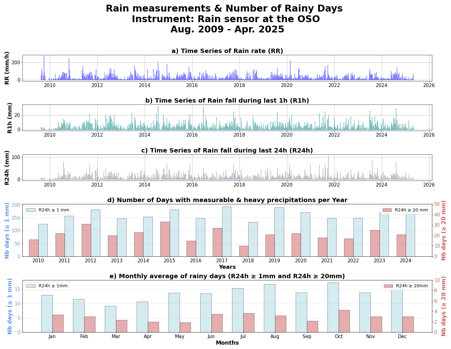
Figure 3 Rainfall measurements and number of days with measurable and heavy precipitation observed at the OSO from August 2009 to April 2025. (a) Time series of rain rate (RR, in mm h⁻¹). (b) Time series of accumulated rainfall over 1 h (R1h, in mm). (c) Time series of accumulated rainfall over 24 h (R24h, in mm). (d) Annual number of days with measurable (R24h ≥ 1 mm; blue bars) and heavy precipitation (R24h ≥ 20 mm; red bars). (e) Monthly number of days with measurable and heavy precipitation, using the same thresholds and color coding as in panel (d).

Rain events are irregularly distributed in time but occur consistently across the 15-year record. Instantaneous rain rate (RR) peaks can exceed 200 mm h⁻¹, although such extremes are infrequent. Rainfall extremes exceeding 50 mm in 24 h are rare but recurrent, aligning with the heavy precipitation thresholds defined previously or by regional climatologies (e.g. Donat et al., 2014; Plauchu-Frayn et al., 2020).

Panel (d) quantifies the annual number of rainy days, distinguishing between measurable precipitation events (R24h ≥ 1 mm, blue bars, left axis) and heavy rainfall events (R24h ≥ 20 mm, red bars, right axis). The number of rainy days (R24h ≥ 1 mm) remains relatively stable over the years (typically between 120 and 180 d yr⁻¹), while heavy rainfall days (R24h ≥ 20 mm) show greater interannual variability, ranging from fewer than 10 d (2018) to over 30 d (2015). These variations are partly associated with interannual shifts in the NAO.

Panel (e) shows the monthly number of rainy days (2010–2024). Measurable precipitation (R24h ≥ 1 mm) occurs most frequently from August to December, with monthly averages reaching up to 15 d. This seasonal maximum reflects increased cyclonic activity during the boreal cold season. Conversely, heavy precipitation (R24h ≥ 20 mm) is most common in autumn, with October exhibiting the highest frequency of such events (up to 5 d per month on average). Spring months (March–May) show lower frequencies of both measurable and heavy rainfall, consistent with reduced synoptic-scale forcing and a greater prevalence of convective, localized events.

Together, these patterns reveal a rainfall regime at OSO characterized by frequent light to moderate precipitation and a smaller number of intense events. The marked seasonal cycle and interannual variability are typical of coastal western Sweden and reflect the site's exposure to North Atlantic storm tracks.

3.5 Wind Regimes and Synoptic Patterns

On the west coast of Sweden, the dominant winds are primarily influenced by the North Atlantic Ocean and regional weather patterns. Figure 4 provides a comprehensive overview of wind conditions recorded at the OSO from August 2009 to April 2025. It includes the site’s geographic context, the overall wind direction and speed distribution (wind rose), seasonal wind patterns, and histograms detailing the frequency of wind direction, wind speed, and gusts. Wind speed and direction measurements at 1 min resolution are used to produce the wind roses and histograms shown. For the seasonal wind roses, data are categorized into four seasons according to the measurement date (see the beginning of Sect. 3 for details).

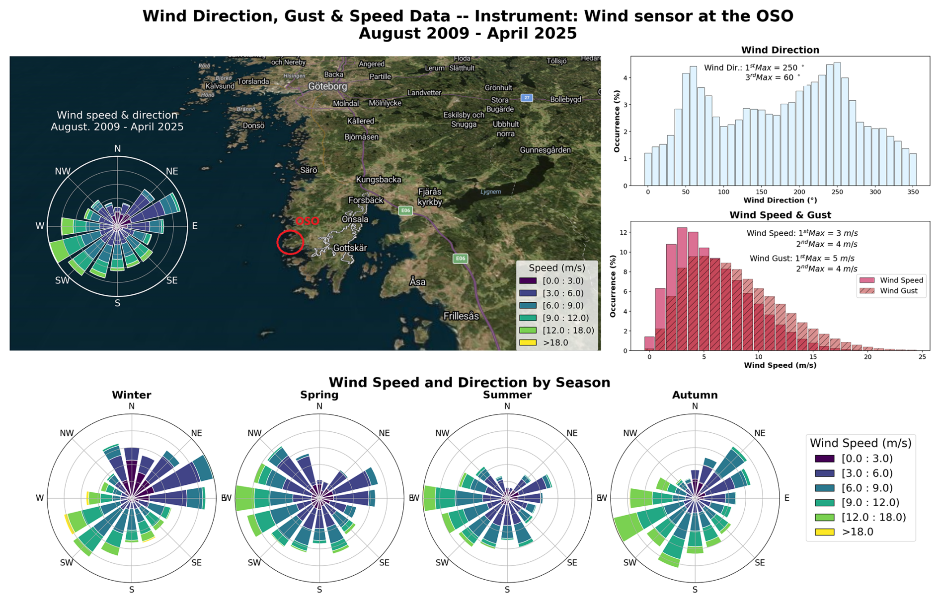
Figure 4 Wind direction and speed recorded at the OSO from 2009 to 2025. The central map (Source: Images © 2025 NASA, Map data © 2025 Google – https://maps.google.com, last access: 6 February 2026) shows the location of the OSO on the Swedish west coast for geographic context. The wind rose diagram (left on the map) displays the distribution of wind direction and speed data (1 min temporal resolution) over the entire period. Top right: Wind direction (in °) histogram (i.e. frequency distribution) and wind speed (solid bars) and wind gust (hatched bars) histogram. Bottom panels: Seasonal wind roses (Winter, Spring, Summer, Autumn). Colours represent different wind speed classes.

The most frequent wind directions are West-Southwest (WSW) and East-Northeast (ENE). WSW winds, originating from the sea, carry marine aerosols and moisture, strongly impacting local thermodynamic conditions. These maritime winds have a moderating effect on air temperatures (especially during winter months) and contribute to cloud formation and precipitation. They also enhance vertical mixing, leading to near-neutral temperature profiles in the lower atmosphere, in contrast to the thermal inversions maintained by the ENE wind conditions. This leads to a reduced diurnal temperature range at the surface.

These dynamics are consistent with broader-scale findings over Central Europe. According to Donat et al. (2010), approximately 80 % of windstorm days in this region are linked to westerly flows, and windstorm occurrence is strongly modulated by the NAO. Most events occur during moderately positive NAO phases, while the rarer strongly positive phases account for over 20 % of all severe windstorm occurrences. These synoptic conditions often favor enhanced cyclonic activity across the North Atlantic, increasing the frequency and intensity of maritime winds reaching Scandinavia.

In contrast, ENE winds are continental in origin and generally dry and cool. These winds are typically associated with anticyclonic weather patterns, which lead to clear skies, strong radiative cooling at night, and warmer daytime temperatures, especially during the spring. These conditions are favorable to temperature inversions, whereby colder air remains trapped near the surface due to a lack of atmospheric mixing.

Figure 4 confirms that the strongest winds – exceeding 10 m s⁻¹ – are predominantly marine (WSW sector), while continental winds are more moderate, often below 6 m s⁻¹. The wind rose also shows that winds can occasionally blow from all directions, although the northern sector contributes little to the overall wind regime.

Overall, the OSO region appears to be dominantly influenced by WSW marine winds and, to a lesser extent, ENE continental winds. Figure B1 shows annual wind roses from 2009 to 2025. Note that data for 2009 and 2025 only cover part of the year (August–December for 2009 and January–April for 2025).

The upper-right panel in Fig. 4 shows that winds most frequently originate from 250° (WSW) and 60° (ENE). In contrast, directions such as true North (0 or 360°) show minimal occurrence. Wind speeds range from 0 to 25 m s⁻¹, with a peak occurrence at 3 m s⁻¹ and most values between 2 and 8 m s⁻¹.

To evaluate seasonal variability, we excluded incomplete years (2009 and 2025). The strongest winds (exceeding 12 m s⁻¹) are observed during autumn and winter, while summer features fewer strong wind events. For all seasons, winds from the eastern half of the compass (land origin) are weaker than those from the west (ocean origin). Seasonal patterns observed in Fig. 4 are as follows:

• Winter. Winds primarily originate from the North and North-Northeast, with stronger winds from the Southwest. These patterns are consistent with earlier studies such as Chen (2000), and align with the cyclonic pathways described by Donat et al. (2010), where storms follow a dominant trajectory from the North Atlantic across the British Isles and southern Scandinavia toward the Baltic Sea.

• Spring. Winds shift to a predominantly westerly origin, still maritime but generally less intense.

• Summer. Winds come from the West and occasionally from the South, with limited influence from the North. This season features the lowest occurrence of strong winds.

• Autumn. Winds return to a Southwest and Northeast pattern. This is a storm-prone season, with frequent strong gusts associated with deep depressions, often enhanced by NAO+ phases.

The influence of the NAO is particularly noticeable in winter. Positive phases (NAO+) are characterized by enhanced zonal flow, bringing mild, wet weather and frequent westerly storms to northern Europe.

3.6 Cloud cover & Solar Irradiance

Figure 5 presents the temporal evolution of solar irradiance (E) measured by the pyranometer, at 1 min resolution, from 2018 to 2025 (top panel), along with its seasonal and diurnal interactions with the cloud cover (lower panel). For the latter, irradiance values corresponding to the exact dates and times of available sky camera observations are used (i.e., every 15 min). It should be noted that E is a direct measurement from the pyranometer, whereas cloud cover (CC) is an estimate. The latter is obtained by calculating the percentage of cloudy pixels in the sky camera image relative to the total number of pixels.

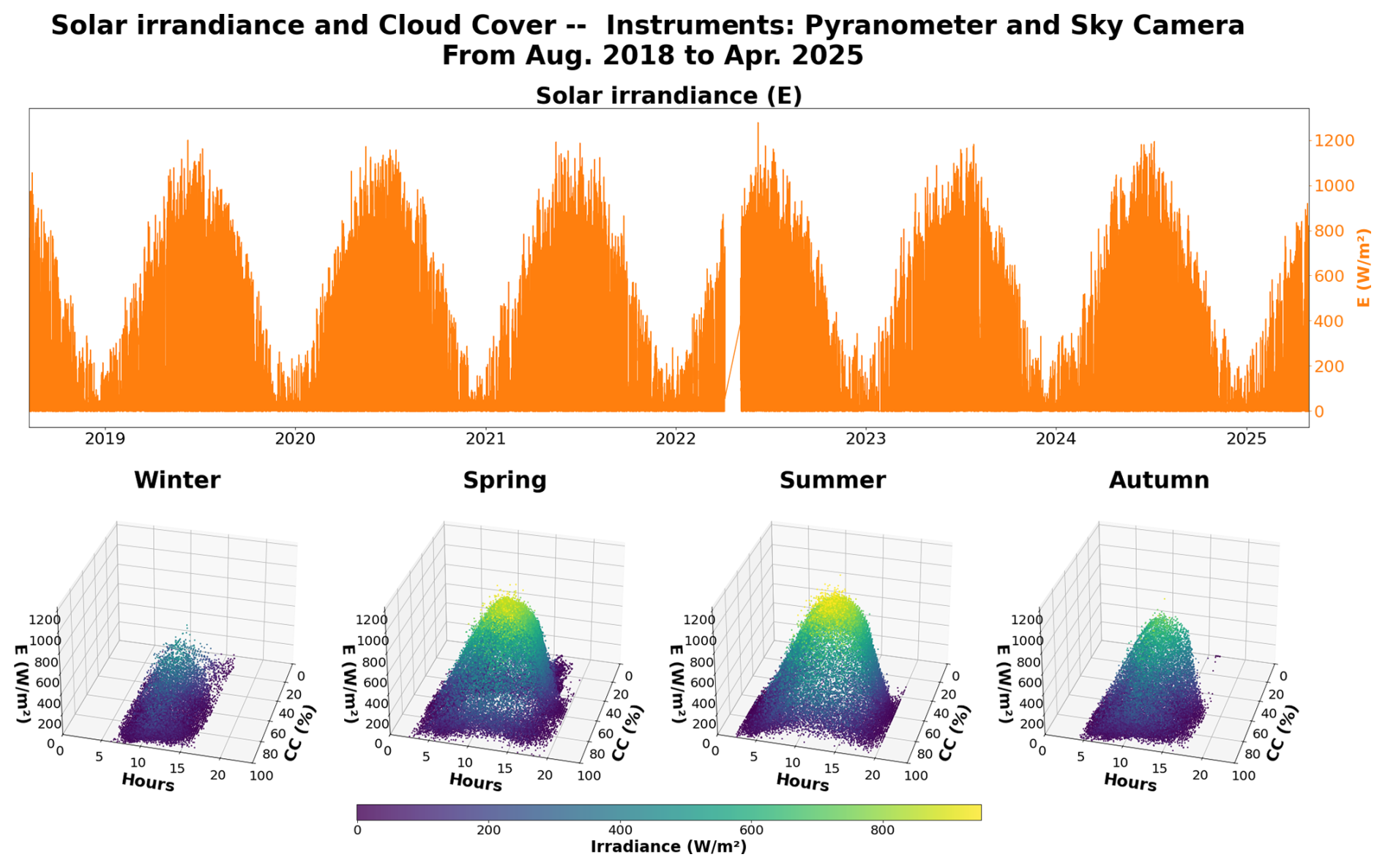
Figure 5 Temporal evolution and seasonal characteristics of solar irradiance (E) and cloud cover (CC), as measured by the pyranometer and estimated from the sky camera. Top panel: Time series of solar irradiance (E, measured every minute, in W m⁻²) from August 2018 to April 2025. Lower panel: 3D scatter plots of E as a function of CC and hour of day for each season (Winter, Spring, Summer, Autumn) between September 2019 and April 2025. For these scatter plots, only data at 15 min resolution are used, corresponding to the CC time step.

The irradiance time series exhibits a clear annual periodicity, with pronounced peaks during the summer months and troughs during winter. Maximum irradiance values exceed 1200 W m⁻² in summer, whereas values frequently fall below 200 W m⁻² in winter, consistent with expected seasonal variations in solar angle and daylight duration. Superimposed on this seasonal cycle are high-frequency fluctuations, largely modulated by cloud cover variability.

The 3D scatter plots (lower panel in Fig. 5) provide insight into the joint distribution of E, CC, and hour of day across the four seasons:

• Winter. Irradiance remains low across all cloud cover conditions, rarely exceeding 600 W m⁻². The time window for significant irradiance is narrow (approximately 09:00 to 15:00), reflecting the short photoperiod.

• Spring. Irradiance levels increase substantially, with maximum values reaching up to 1000 W m⁻². The irradiance distribution broadens with time of day and cloud cover, suggesting a more dynamic range of sky conditions. Clear-sky conditions begin to contribute significantly to total solar energy.

• Summer. This season presents the highest irradiance values and the longest duration of solar exposure, with peak irradiance occurring between 08:00 and 16:00. Despite the presence of high cloud cover in some instances, irradiance often remains elevated, indicating the influence of partially cloudy skies and potential cloud edge enhancement effects.

• Autumn. As solar elevation decreases, irradiance levels and daylight duration both diminish. The pattern is similar to spring but with an overall decline in peak irradiance and a noticeable shift of the irradiance peak toward midday.

Across all seasons, the inverse relationship between CC and E is evident. However, the relationship is non-linear: significant irradiance can still occur under moderate to high CC conditions, especially in summer. This reflects the complex interplay between cloud optical properties, cloud type, and solar geometry. These results highlight the importance of considering both cloud cover and diurnal cycles in solar resource modeling. Seasonal variability plays a critical role not only in the total irradiance received but also in the timing and reliability of solar availability.

4 Inter-annual trends

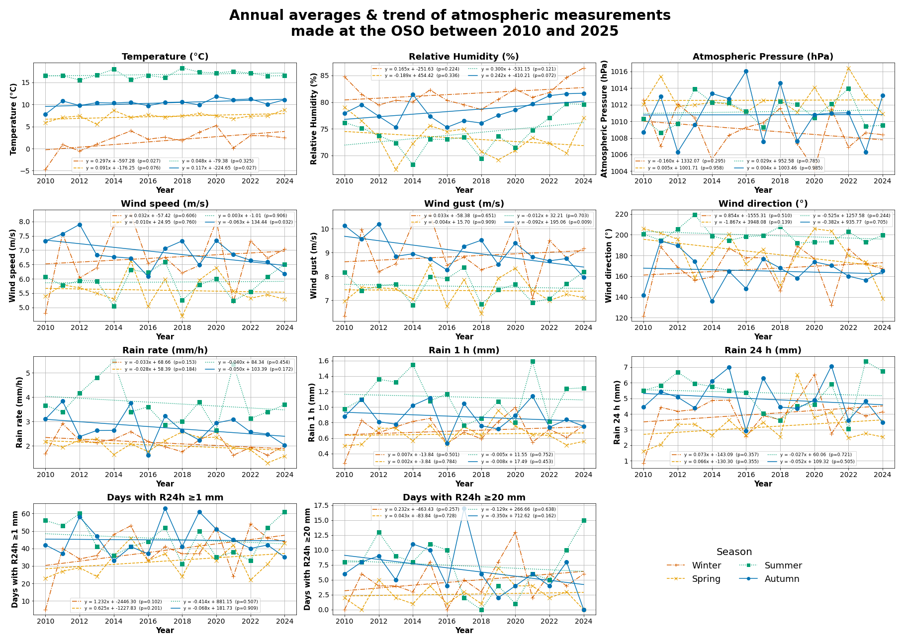
In this section, we analyse the 15-year trends (2010–2024) of the parameters introduced above, excluding cloud cover (CC) and solar irradiance (E) for which less than five complete years of data are available. We consider only full calendar years (2010–2024) and compute trends based on annual mean values.

Figure 6 displays the annual averages of each parameter together with their linear regression fits. Table 2 reports the slope (a) and intercept (b) of the regression model a x+b (with $x=\mathrm{1},\mathrm{2},\mathrm{\dots },N$ years) alongside the associated p-values. Cells highlighted in bold correspond to p-values ≤0.05, indicating statistical significance at the 95 % confidence level. In addition, Table 2 also includes the Root Mean Square Error (RMSE) of each linear regression. RMSE quantifies the average deviation of the observed annual means from the fitted trend line and serves as an indicator of how well the fit captures interannual variability.

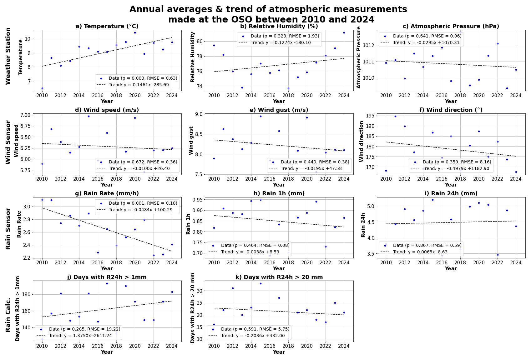
Figure 6 Annual mean values and linear trends of atmospheric variables recorded at the OSO from 2010 to 2024. Panels (a)–(c) show (a) temperature, (b) relative humidity, and (c) atmospheric pressure; panels (d)–(f) display wind characteristics: (d) wind speed, (e) gust speed, and (f) wind direction; panels (g)–(i) present precipitation metrics: (g) rain rate, (h) total rainfall in 1 h, and (i) total rainfall in 24 h; and panels (j)–(k) summarize rainfall occurrence: (j) number of days with R24h ≥ 1 mm and (k) days with R24h ≥ 20 mm. Dotted lines denote the best‐fit linear trends, and p-values and RMSE for trend significance are indicated in each panel’s legend.

Table 2 Linear annual trends (2010–2024) of meteorological parameters measured at the Onsala Space Observatory with: slope a (± standard deviation), intercept b (± standard deviation), p-value, RMSE, and indication of statistical significance. Bold font indicates parameters with statistical significance at a 95 % confidence level.

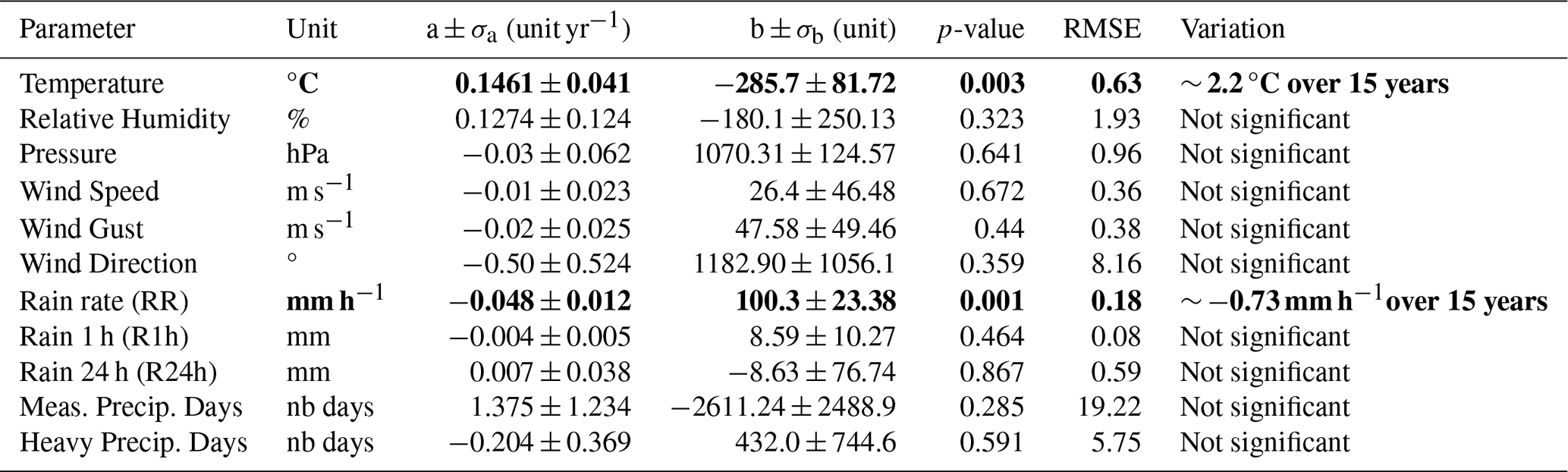
Annual mean air temperature exhibits a robust warming of +0.1461 °C yr⁻¹ (p=0.003, RMSE =0.63), raising the 2010–2024 average from 6.5 to ∼ 9.75 °C. Over the 15-year period, this corresponds to an increase of about 2.2 °C in the annual average temperature – a significant warming trend that may reflect broader regional or global climate warming patterns (IPCC, 2022; Dankers and Hiederer, 2008).

For relative humidity, the fitted line suggests a slight increase over time, but with a p=0.323, meaning the variation is not statistically significant. When looking at the annual averages point by point, a pattern of alternating decreases and sharp increases appears to be present. A visible offset is observed in the annual cycles since 2018 (Fig. 2e), where average monthly RH values appear higher than in the previous decade. While the absence of sensor recalibration since 2009 means an instrumental drift cannot be definitively ruled out, this variation is partially concurrent with a significant increase in surface temperature (p=0.003, Fig. 6a) and an increase in the frequency of light rain days (Fig. 6j). Furthermore, the scarcity of foggy days at OSO is consistent with the recorded data, and the physically coherent diurnal anomalies (Fig. 2g) suggest that the sensor maintains sufficient sensitivity for process-based analysis.

Regarding atmospheric pressure, the slope is slightly negative but not statistically significant (p=0.64). The annual mean pressure appears stable over this period, showing no meaningful long-term change.

Wind sensor data indicate marginal decreases in annual mean wind speed (−0.01 m s⁻¹ yr⁻¹, p=0.672) and gust magnitude (−0.02 m s⁻¹ yr⁻¹, p=0.44). None of the wind‐related trends attain conventional significance, pointing to natural variability as the dominant control.

Precipitation intensity (RR) exhibits a clear downward trend over the study period. The mean rain rate decreases significantly by −0.05 mm h⁻¹ yr⁻¹ (p=0.001), amounting to ∼ −0.73 mm h⁻¹ over 15 years. This statistically significant decline indicates a measurable reduction in short-term rainfall intensity; however, the dispersion remains within the instrumental margin of error (RMSE =0.18). In contrast, 1 h rainfall accumulations show a slight, non-significant decrease of −0.004 mm yr⁻¹ (p=0.464), while 24 h totals exhibit a negligible and non-significant increase of +0.0065 mm yr⁻¹ (p=0.867). The frequency of precipitation days does not exhibit statistically significant changes. The number of days with measurable precipitation (R24h ≥ 1 mm) shows a slight increase, while the number of days with heavy precipitation (R24h ≥ 20 mm) shows a small decrease, both variations being statistically non-significant.

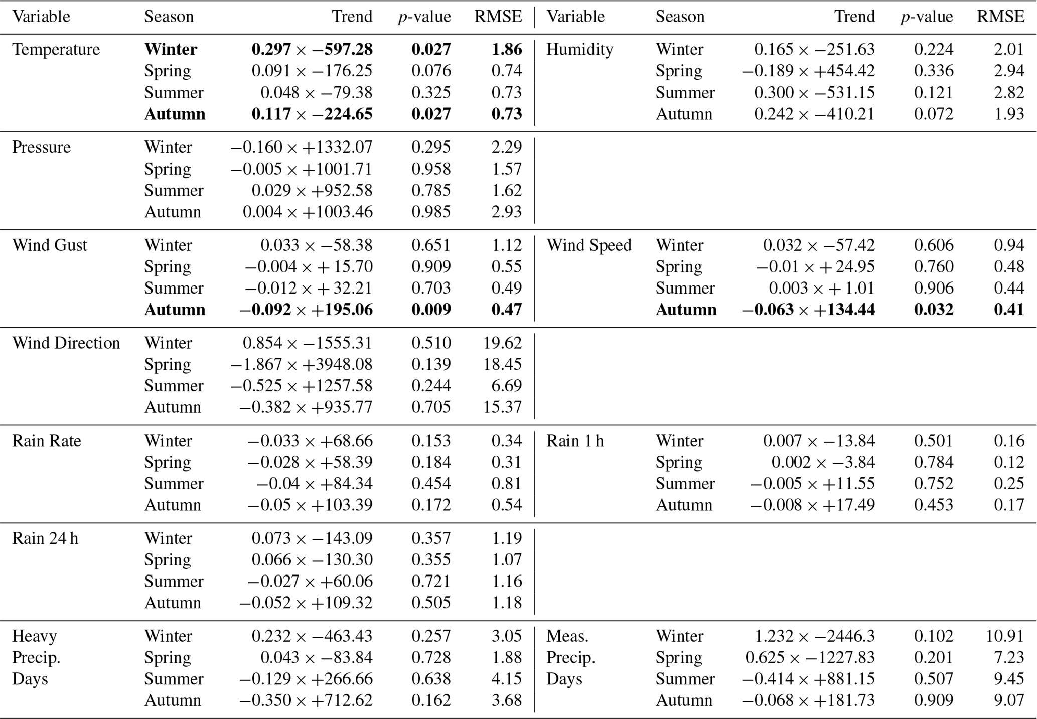
As an indication, the linear regression trends for seasonal averages has been calculated. This will help determine whether one season is more affected than another by climate change or if an inter-seasonal compensation is visible. Figure C1 and Table C1 show the seasonal averages and their associated trends for each parameter. The p-values indicating a trend with a confidence level up to 95 % (p≤ 0.05) are:

• For temperature:

  • –

    in autumn (p ∼ 0.03), the trend shows an increase of 0.12 °C yr⁻¹ (which corresponds to ∼ 1.76 °C over 15 years).

  • –

    in winter (p ∼ 0.03), the increase is ∼ 0.3 °C per year (∼ 4.5 °C over 15 years).

  Although not statistically significant, temperature trends are also increasing for the other two seasons (spring and summer). However, the most pronounced temperature increase occurs in winter (203.3 % compared to the annual trend). The deviation from the annual trend then decreases in autumn (80.1 %), spring (62.3 %), and summer (32.9 %).

• For wind:

  • –

    wind speed, in autumn (p ∼ 0.03): an upward trend is observed (−0.063 m s⁻¹ per year, which corresponds to −0.95 m s⁻¹ over 15 years).

  • –

    wind gust, in autumn (p ∼ 0.009): the decrease is ∼ 0.1 m s⁻¹ per year (∼ −1.4 m s⁻¹ over 15 years).

  Regarding wind speed, the declining trend in autumn seems to be compensated by an increase in winter, with almost no variation in spring and summer. However, the linear fit has a high p-value (especially for data in summer), so no strong conclusion can be drawn. We observe the same kind of pattern for the seasonal trends of wind gusts.

For rain rate, no season shows a trend with a statistically significant p-value. However, the rain rate tends to decrease in all seasons, which explains why the trend is significant for annual averages. Note that the maximum values are recorded in autumn and summer.

In conclusion, between 2010 and 2024, the OSO station’s Vaisala WXT520 record reveals that the increase in temperature is more pronounced in winter than in the other seasons and that the downward trend in the rain rate is evident (but low) throughout the year. The absence of significant trends in the other parameters further highlights the complexity and multifactorial nature of local climate variability.

5 Data availability

The data described in this manuscript are available through PANGAEA: (1) Ground-based meteorological measurements at the Onsala Space Observatory (Sweden) between 2009 and 2025; (https://doi.org/10.1594/PANGAEA.984087, Mascaut et al., 2026a); (2) Ground-based atmospheric solar radiation measurements at the Onsala Space Observatory (Sweden) between 2009 and 2025. (https://doi.org/10.1594/PANGAEA.984085, Mascaut et al., 2026b). The complete citations are provided in the reference list (Mascaut et al., 2026a, b).

In all time series, the first column represents UTC date and time, with the format yyyy-mm-ddThh:mm:ss. The columns are separated by tabs (\t). Note that basic quality control was applied to the data and no gap filling or homogenization was applied. A detailed file description is provided in Table 1.

The record of NAO phases from 1950 to present is available from NOAA's Climate Prediction Center (https://www.cpc.ncep.noaa.gov/products/precip/CWlink/pna/nao.shtml, last access: 7 May 2025).

6 Conclusions

We analysed more than 15 years of continuous, high-resolution ground-based atmospheric measurements collected at the Onsala Space Observatory (OSO), located on the Swedish west coast, from August 2009 to April 2025. The dataset includes minute-scale records of near-surface (16.1 m a.s.l.) air temperature, relative humidity, atmospheric pressure, precipitation (rain rate, 1 and 24 h accumulations), sustained wind speed, gusts, and direction as weel as solar irradiance at 12 m a.s.l. All variables were quality-controlled and analysed statistically. In addition to descriptive analyses, we explored seasonal cycles, interannual variability, and linear trends, and we related key anomalies to the phase of the NAO. Our results confirm several consistent signals:

• Temperature. A statistically significant warming trend of +0.15 °C per year was detected, with winter warming reaching approximately 203 % above the annual mean rate. The warming signal was most pronounced between 2013 and 2020, and is consistent with Arctic amplification patterns and regional trends reported in Northern Europe.

• Precipitation. While accumulated precipitation (over 1 or 24 h) showed no clear trend, we observed a slight but significant decline in rain rate intensity over the study period (−0.05 mm h⁻¹ yr⁻¹). The frequency of wet days (R24h ≥ 1 mm) remained relatively stable across years, while the number of heavy precipitation days (R24h ≥ 20 mm) showed greater interannual variability. Seasonal analyses confirmed summer and autumn as the wettest seasons, and spring as the driest.

• Wind. Westerly (WSW) maritime flows dominate the wind data, with wind roses showing stronger wind speeds and gusts during winter and autumn months. Windstorm activity was found to correlate with NAO phase, with most events occurring under moderately or strongly positive NAO conditions. The mild winter of 2019–2020, for instance, coincided with a positive NAO phase, while the cold winter of 2009–2010 occurred during a strong negative NAO phase.

• Pressure. Atmospheric pressure displayed clear semidiurnal tides, consistent with theoretical expectations and prior studies. The timing and amplitude of pressure oscillations showed seasonal modulation, particularly in the timing of the secondary minima.

• Solar irradiance. Solar irradiance followed well-defined seasonal and daily cycles, with maxima in summer and minima in winter. Despite an overall inverse relationship with cloud cover, significant irradiance can still occur under moderate cloud conditions, especially in summer.

Together, these observations provide a valuable benchmark for understanding local expressions of broader climate dynamics. Although this dataset is geographically limited, it captures key processes relevant to Northern European coastal climates, including land–sea interactions, mid-latitude storm tracks, and NAO-related variability. By making this dataset publicly available, we aim to support further research in regional trend attribution, model evaluation, and synoptic climatology.

Appendix A: North Atlantic Oscillation (NAO) phases

The data and information in this appendix are sourced from the NOAA website (https://www.cpc.ncep.noaa.gov/products/precip/CWlink/pna/nao.shtml, last access: 7 May 2025). Figure A1 shows the monthly NAO index values between 2009 and 2025. The data for the winter months (December, January, and February) are highlighted: red indicates a negative index (NAO−) and dark blue indicates a positive index (NAO+).

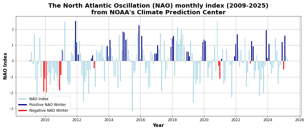
Figure A1 The monthly index of the North Atlantic Oscillation between 2009 and 2025. Data from NOAA's Climate Prediction Center.

Table A1 presents the impact of the NAO phase (positive or negative) on the local weather in our study region (the west coast of southern Sweden).

Table A1 Impacts of NAO Phases on Weather along the West Coast of Sweden, by Season. Source: NOAA Climate.gov, “Climate Variability: North Atlantic Oscillation” (2009).

Appendix B: Wind Speed and Direction by Year

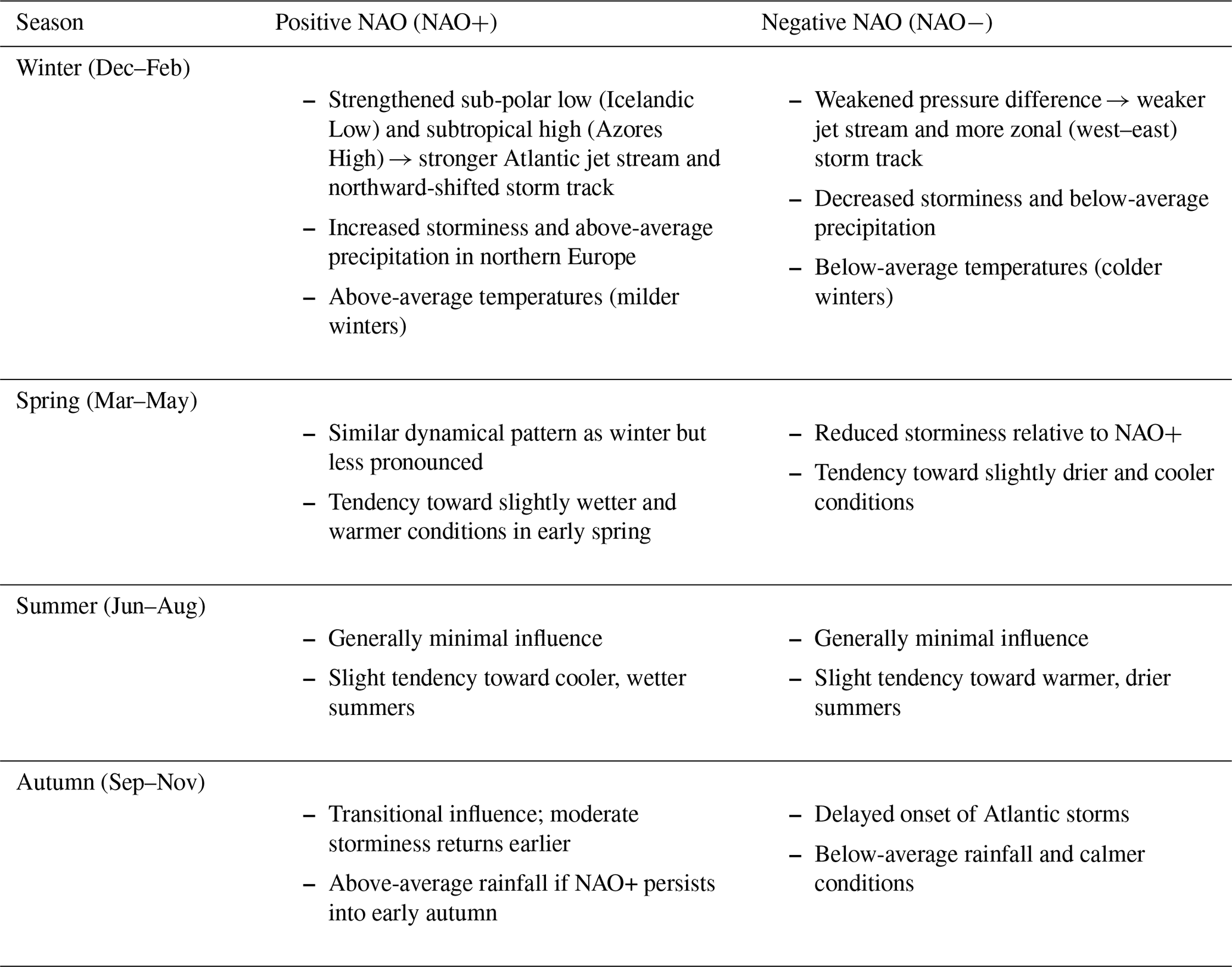
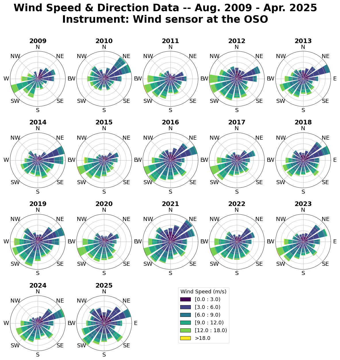
Figure B1 Annual wind‐rose diagrams depicting the distribution of wind direction and speed from August 2009 to April 2025. Each panel represents one calendar year (2009–2025). Note that 2009 and 2025 are not complete years.

Appendix C: Inter-annual trends by season

Figure C1 Same as Fig. 6 but for each season: winter in red, autumn in blue, spring in orange and summer in green.

Table C1 Linear annual trends (2010–2024), p-value and RMSE from the Fig. C1. Bold font indicates parameters with statistical significance at a 95 % confidence level.