An accurate 10 m annual crop map product of maize and soybean across the United States

High-resolution crop maps over large spatial extents are fundamental to many agricultural applications; however, generating high-quality crop maps consistently across space and time remains a challenge. In this study, we improved a workflow for crop mapping and developed an openly available, annual, 10 m spatial resolution maize and soybean map product over the Contiguous United States (CONUS) from 2019 to 2022 (available at https://glad.umd.edu/dataset/mapping-crops-10-m-resolution-united-states, last access: 26 December 2025). We obtained all available Sentinel-2 surface reflectance data between May and October for every year, applied quality assurance, corrected the bidirectional reflectance distribution function (BRDF) effects, and generated 10 d analysis ready data (ARD) composites. We then derived multi-temporal metrics from the 10 d ARD as training features for the national-scale wall-to-wall mapping. We implemented a stratified, two-stage cluster sampling, and then conducted annual field surveys and collected ground data. Utilizing the training data with Sentinel-2 multi-temporal metrics and topographic factors, we trained random forest models generalized for annual maize and soybean classification separately. Validated using field data from the two-stage cluster sample, our annual maps achieved consistent overall accuracies (OA) greater than 95 % with standard errors of less than 1 %. User's accuracies (UAs) and producer's accuracies (PAs) for maize were higher than 91 % and 84 % across the years, and UAs and PAs for soybean were greater than 88 % and 82 %, respectively. To illustrate the substantial improvement of the 10 m map over existing datasets, e.g., the 30 m Cropland Data Layer (CDL), we aggregated the 10 m maps to 30 m spatial resolution and quantified the number of mixed pixels that can be reduced by improving the mapping from 30 to 10 m. The counties with the most maize and soybean production in Iowa, Illinois and Nebraska had the lowest reduction in mixed pixels, ranging from 1 % to 7 %, whereas southern counties had a higher reduction in mixed pixels. Overall, the median percentages of mixed maize and soybean pixels reduction across all counties were 8 % and 9 %, respectively. With more Sentinel-2-like data available from continuous observations and incoming satellite missions, we anticipate that 10 m crop maps will greatly benefit long-term monitoring for agricultural practices from the field to global scales. The dataset is also available at https://doi.org/10.6084/m9.figshare.28934993.v2 (Li et al., 2025).

1 Introduction

Satellite-derived crop maps are essential to many agricultural applications, such as crop yield prediction (Bolton and Friedl, 2013; Song et al., 2022; Wang et al., 2024), food market forecasting (Tanaka et al., 2023), crop area estimation (Khan et al., 2016), conservation policy design (Song et al., 2021b; Zalles et al., 2021), smallholder livelihood evaluation (Lambert et al., 2018), warfare impacts on food security (Li et al., 2022; Lin et al., 2023), and greenhouse gas emissions in agriculture (Escobar et al., 2020; Ouyang et al., 2023). However, along with these benefits are the outstanding challenges to generating high-quality crop maps, including developing consistent ready-to-use satellite datasets, collecting representative field data, and building classification algorithms robust to phenological variations.

Dense time series of satellite observations with complete spatial coverage is essential to mapping crops at broad scales. With global coverage and daily revisit frequency, the Moderate Resolution Imaging Spectroradiometer (MODIS) data are often used for crop mapping in early studies (Wardlow et al., 2007; Wardlow and Egbert, 2008). However, spatial details within individual small fields can rarely be depicted at 250 m resolution (Fritz et al., 2015), especially for more than 475 million smallholder and family farms accounting for 12 % of the world's agricultural land (Lowder et al., 2016). Since the opening of the Landsat archive in 2008 (Woodcock et al., 2008), Landsat data have been extensively used to generate 30 m crop maps in many parts of the world, such as in North America (Boryan et al., 2011; Fisette et al., 2013; Johnson and Mueller, 2021; Song et al., 2017; Wang et al., 2020), Europe (Foerster et al., 2012), South America (Song et al., 2021b), and Asia (Dong et al., 2016; Khan et al., 2021; Remelgado et al., 2020). However, Landsat-based crop mapping is hampered by the relatively sparse 16 d temporal frequency (8 d with two satellites), especially when cloudy weather persists. Compared to Landsat, Sentinel-2A and -2B together have a revisit frequency of 5 d and provide 10, 20 and 60 m spectral bands including red edge bands that are particularly useful for crop identification (Immitzer et al., 2016; Song et al., 2021a). These advantages make Sentinel-2 data one of the best publicly accessible data sources for crop mapping (Ghassemi et al., 2022; Han et al., 2021; Luo et al., 2022; You et al., 2021).

Crop classification from satellite imagery is usually implemented by relating specific crop types to remotely sensed features, using reference data and classification algorithms such as conventional machine learning or advanced deep learning (e.g., Alami Machichi et al., 2023; Joshi et al., 2023). Therefore, in situ data can serve as critical references to annotate satellite imagery for supervised classifications, although field surveys over large areas require extensive time and labor resources. Currently, the US Department of Agriculture (USDA) National Agricultural Statistics Service (NASS) collects periodic field data across the US and produces the Cropland Data Layer (CDL) annually based on a large amount of ground data and supervised algorithms (Boryan et al., 2011). When current-year labels are unavailable, some researchers have explored transferring pre-trained models to target regions or years (Luo et al., 2022; Wang et al., 2019), or generating labels with knowledge-guided approaches (Lin et al., 2022; You et al., 2023). However, these approaches are limited to experiments at small spatial scales, such as the US Midwest and Northeast China, and thus the efficiency of national-scale crop classification over large countries with more challenging environments remains to be explored. In cases where reference data are entirely unavailable, unsupervised classifications are used first to cluster satellite-derived features and then assign crop labels to the clusters to generate approximate crop maps (Konduri et al., 2020; Xiong et al., 2017). They, however, are vulnerable to outliers and noisy features and require intensive visual inspections (Wang et al., 2019). In summary, collecting representative ground data is a critical yet challenging component for large-area crop mapping.

Spatiotemporal consistency in crop classifications is necessary to make annual crop maps comparable and thus allow long-term crop monitoring and change analysis. Yet this is undermined partly due to crop phenology variations across large extents, depending on soil properties, planting dates, and weather conditions, among other factors (Deines et al., 2023; Yang et al., 2017). On one hand, within a calendar year, crop progress is regionally different. To address this issue, some studies trained regional models through agroecological zoning, which requires zone-specific training and validation (de Abelleyra et al., 2020; Wardlow and Egbert, 2008). On the other hand, yearly unaligned phenological profiles can jeopardize the classification consistency across years, especially when extreme weather events occur (Manoochehr et al., 2021). Given these interannual variations, classifiers that accurately identify crops in average normal growing seasons using single-date or time-series satellite imagery may perform poorly for abnormal years. To this end, researchers proposed yearly specific classifications (Massey et al., 2017; Som-ard et al., 2022). However, these annual models need fine-tuning based on reference data from each corresponding year especially when encountering unseen growing trends, and thus cannot be generalized for long-term periods.

Multi-temporal metrics are statistical transformations of temporal profiles of satellite observations that can improve spatial and temporal consistency and facilitate land cover mapping for large areas. In the mid-1980s, researchers derived phenological features from pixel time series from the Advanced Very High Resolution Radiometer (AVHRR) for vegetation monitoring (Malingreau, 1986) and from Landsat Multispectral Scanner (MSS) for crop classification (Badhwar, 1984). This metrics method was then widely used for land cover mapping and change analysis from regional to global scales using AVHRR, MODIS and Landsat data (DeFries et al., 1995; Hansen et al., 2013; Potapov et al., 2021b; Song et al., 2018). For crop mapping over continental scales, the metrics method was used to generalize classification models robust to interannual phenological variations (Song et al., 2021b). Many studies are adopting similar concepts for regional crop mapping (Kerner et al., 2022; Konduri et al., 2020; Yang et al., 2023; Zhong et al., 2014).

In the US, the CDL has been used widely for many applications (Bolton and Friedl, 2013; Gao et al., 2017; Lobell et al., 2020; Wright and Wimberly, 2013; Yan and Roy, 2016). Recently, the 2024 CDL has been successfully released with the spatial resolution increased from 30 to 10 m (https://www.nass.usda.gov/Research_and_Science/Cropland/SARS1a.php, last access: 26 December 2025). However, the previous years of CDL are at 30 m resolution, and have inconsistent accuracies depending on the location, and inaccurate classifications are observed in sparse or complex agricultural regions (Larsen et al., 2015). The 30 m spatial resolution can lead to substantial mixed pixels, obscuring incremental or pixel-level changes, particularly along field boundaries. In comparison, 10 m maps with a higher spatial resolution can improve the delineation of precise field boundaries, reducing mixed pixels in individual fields, as well as lowering uncertainties of area estimation. Global 10 m crop mapping efforts are rare, although the WorldCereal provides an example (Van Tricht et al., 2023). In Europe, recent 10 m crop mapping efforts include the Crop Map of England (CROME) (CROME, 2024), the parcel-level crop maps in the Netherlands (ESA, 2024), the crop maps produced by the Sentinel-2 for Agriculture (Sen2-Agri) (Defourny et al., 2019; Inglada et al., 2015), and the more recent High Resolution Layer Crop Types (CTY) (EU, 2024). In Asia, large-area crop-specific maps have been generated recently (Han et al., 2021; Li et al., 2023; Mei et al., 2024). In the US, the potential of national-scale 10 m crop mapping has rarely been explored, although a recent prototyping effort has been reported (Huang et al., 2024).

The objective of this study is to develop annual 10 m crop maps with Sentinel-2 time series. We also quantify the benefits of 10 m maps compared to existing 30 m products. In this study, we generated annual maize and soybean maps at 10 m spatial resolution over the entire Contiguous US (CONUS), from 2019 to 2022. We also quantified the benefits of our 10 m crop maps in mixed pixel reduction compared to 30 m maps, at field, regional and national scales. We improved a workflow developed in previous studies (Li et al., 2023; Song et al., 2017) by combining satellite analysis ready data (ARD) generation, field survey design, and machine learning. An overview workflow for annual crop map production is presented in Fig. 1.

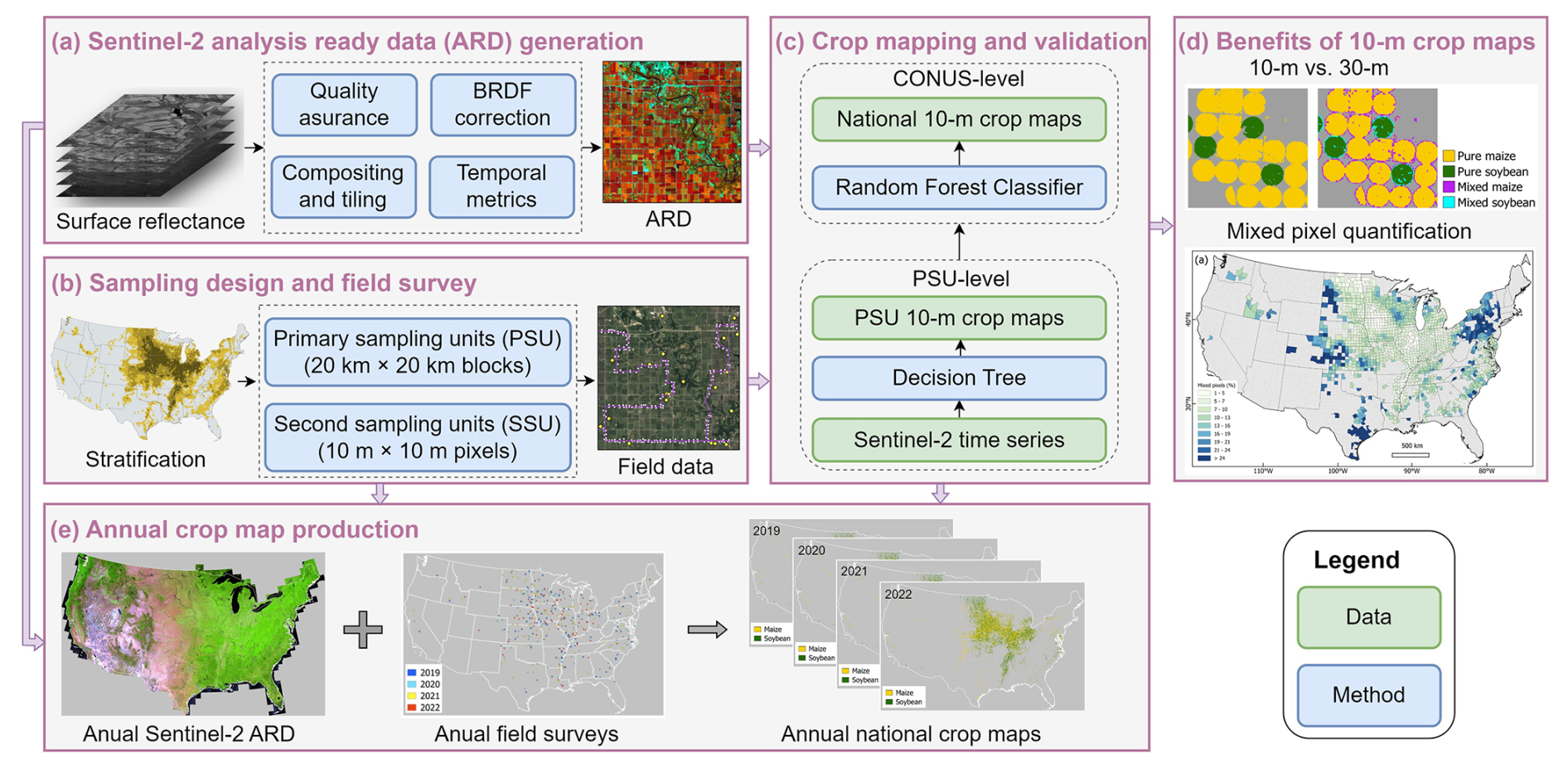
Figure 1 Overview of the workflow for large-area annual crop map production.

2 Materials and methods

2.1 Satellite analysis ready data (ARD) generation

Operational crop mapping over large areas relies on satellite data that are geometrically and radiometrically consistent with quality assessment (e.g., Boryan et al., 2011; Fisette et al., 2013; Song et al., 2021b). Analysis ready data (ARD), defined by the Committee on Earth Observation Satellites (CEOS), meet such criteria as “have been processed to a minimum set of requirements and organized into a form that allows immediate analysis with a minimum of additional user effort and interoperability both through time and with other datasets” (https://ceos.org/ard/, last access: 11 November 2024). To support annual wall-to-wall crop mapping over the CONUS, we obtained all available Sentinel-2 data between May and October, applied quality assurance, corrected the bidirectional reflectance distribution function (BRDF) effects, and generated 10 d ARD composites.

We downloaded Sentinel-2A and -2B Level-2A Bottom of the Atmosphere reflectance (S2 L2A) images from Google Cloud, including the 10 m blue, green, red and near-infrared (NIR) bands, the 20 m red edge (RE1, RE2, RE3), narrow near-infrared (NNIR) and shortwave infrared (SWIR1, SWIR2) bands. We selected images acquired between 1 May and 31 October after filtering out images with >80 % cloud cover. We then processed all available Sentinel-2 data by utilizing the GLAD and Zaratan high-performance computing clusters at the University of Maryland and generated Sentinel-2 ARD for the wall-to-wall crop mapping. Details of the ARD generation are described in the following sections.

2.1.1 Quality assurance

Based on the S2 scene classification (SCL) layer, we generated the cloud mask by merging categories of cloud shadow, thin cirrus, snow, cloud with low, medium and high probability into cloudy pixels. We also produced an additional cloud mask layer derived from the Fmask algorithms (Zhu et al., 2015) and the Cloud Displacement Index (Frantz et al., 2018). We combined the SCL-derived cloud mask with the additional cloud mask as the final quality assurance (QA) layer.

2.1.2 Bidirectional Reflectance Distribution Function (BRDF) correction

We corrected the BRDF effects using the c-factor method to derive nadir BRDF-adjusted reflectance (NBAR) (Roy et al., 2017a, b). The S2 L2A product provides solar and view geometry metadata in 23 × 23 grids at 5 km spatial resolution. For each multi-spectral instrument (MSI) detector in each spectral band, the solar zenith and azimuth angles remain consistent; the view zenith and azimuth angles, however, vary from one detector to another, and from band to band. We calculated the mean value of the view zenith and azimuth angle for each 5 km grid across all detectors and all spectral bands. Per-pixel solar and view angles at 10 m resolution were derived by nearest neighbor interpolation of the 5 km grid values. As a result, the 10 m angle layers were used to generate NBAR images using the global spectral BRDF model parameters (Roy et al., 2017a, b). This process reduced the BRDF effects and improved the spatial coherence compared to the surface reflectance without BRDF correction (Fig. 2).

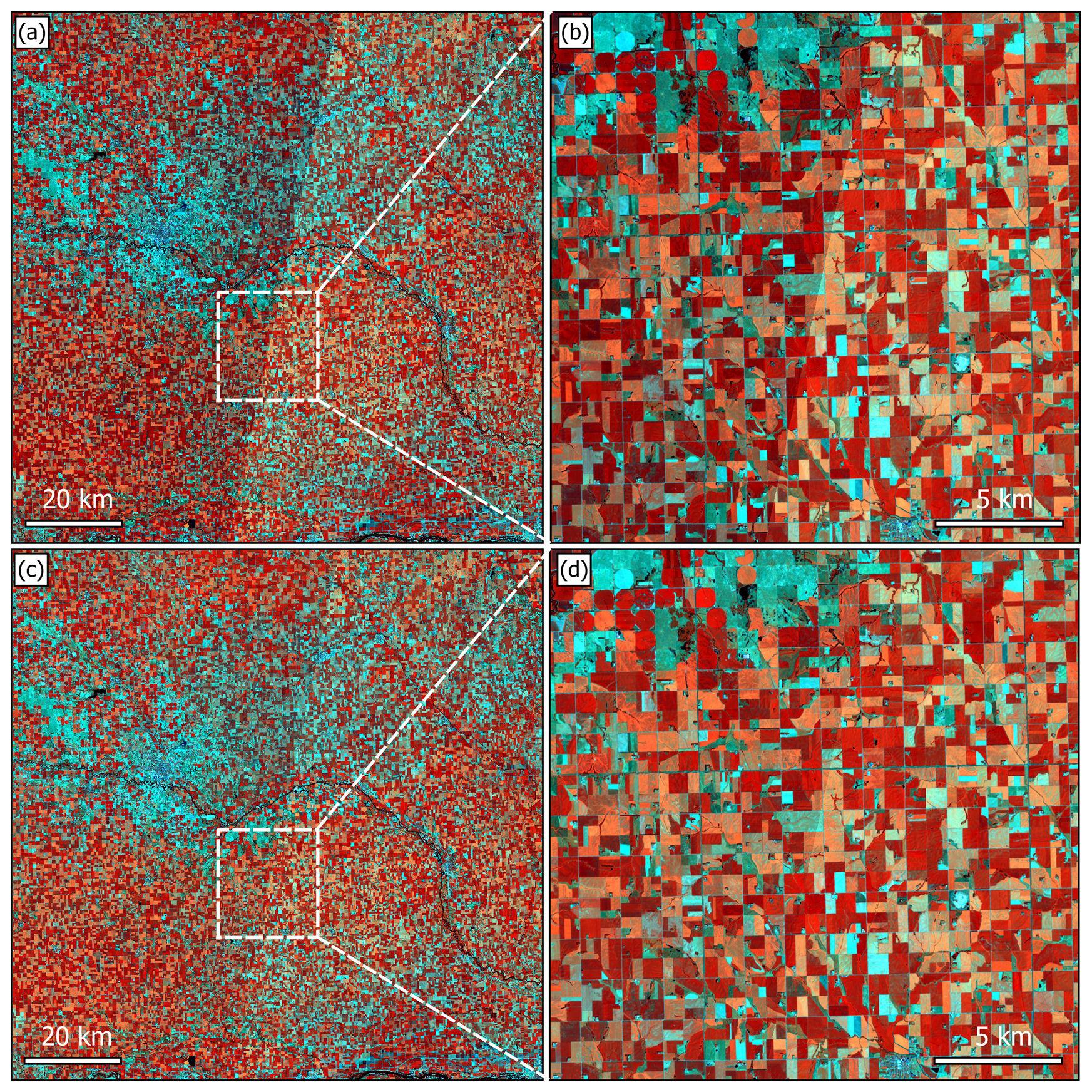
Figure 2 Sentinel-2 false color composites (R: NIR, G: SWIR1, B: SWIR2) over a selected UTM tile 14TMP centered at (97.131° W, 41.942° N). (a–b) Surface reflectance. (c–d) Nadir BRDF-adjusted reflectance (NBAR). Two overlapping Sentinel-2B swaths acquired from orbit R112 on 18 July 2022 (backscattering direction) and orbit R012 on 21 July 2022 (forward scattering direction) were used. The orbit R112 data were overlaid on the orbit R012 data where they overlapped. All composites are displayed with the same stretch parameters. Figure contains modified Copernicus Sentinel data (2022).

2.1.3 Temporal composition and tiling

We resampled the 20 m bands to 10 m using the nearest neighbor method, applied the QA layer, and created 10 d median composites. For each NBAR band in a given 10 d interval, the median value of all clear-sky observations and the corresponding day of the year (DOY) were selected. We also implemented temporal linear interpolation on a per-pixel basis to fill the data gaps (Griffiths et al., 2019). For a missing value in a 10 d interval, the gap-filled value was calculated from the preceding and subsequent valid observations. A maximum of six 10 d intervals (i.e., 60 d or 2 months) was used to limit the period so that the interpolation was temporally relevant. For cases in which cloud-free observations are unavailable for two months, we did not conduct interpolation.

We divided the entire study area into 1° × 1° non-overlapping tiles in geographic latitude/longitude projection with WGS84 datum. Each tile was named by the latitude and longitude coordinates of the lower-left corner, with 0.0001° × 0.0001° spatial resolution to approximately match a 10 m pixel of Sentinel-2. We reprojected 1028 Sentinel-2 Universal Transverse Mercator (UTM) tiles into 939 1° × 1° tiles over the United States.

2.1.4 Multi-temporal metrics

The 10 d S2 ARD may have inconsistent observational frequencies across space and time depending on the geographical location and cloud condition. Generating multi-temporal metrics from ARD can improve data consistency, and thus enable large-area land cover mapping, which has been demonstrated in various applications at continental and global scales (Hansen et al., 2013; Potapov et al., 2021a; Song et al., 2021a).

Following the method in Potapov et al. (2020), we generated multi-temporal metrics from the 10 d S2 ARD (see Table S1 in the Supplement). First, we derived the Normalized Difference Vegetation Index (NDVI, (NIR − Red)$/$(NIR + Red)) (Tucker, 1979) and the normalized ratio between shortwave infrared bands (SWSW, (SWIR1 − SWIR2)$/$(SWIR1 + SWIR2)) from corresponding NBAR bands. Second, we ranked time-series observations by each NBAR band or index individually. We then selected the second maximum, the second minimum, and median values per pixel, and calculated the 10th, 25th, 75th, and 90th percentiles. We also calculated the average, standard deviation, and amplitude between these percentiles and the second maximum, the second minimum values. Third, we ranked the observation day of year (DOYs) according to the time-series NDVI, and derived values on the DOYs corresponding to the second maximum, the second minimum, and median, as well as the 10th, 25th, 75th, and 90th percentiles of NDVI values. The average, standard deviation and amplitude were also calculated from these extracted values.

In total, we calculated 621 metrics. The NBAR averages between the 25th and 75th percentiles from observations ranked by individual bands are illustrated in Figs. 3 and 4a. The NBAR amplitudes reveal land surface phenology and thus simplify visual interpretation of general land cover types such as cropland, open water, forest, and wetland (Fig. 4b). When the averages are calculated from observations with the highest NDVI values (between 90th percentile and the second maximum NDVI value), the composite shows surface reflectance during the peak growing season, improving the identification of multiple crop types (Fig. 4c and d).

Figure 3 Sentinel-2 composites over the United States in 2022. The composites were created using the average value of nadir Bidirectional Reflectance Distribution Function (BRDF)-adjusted reflectance (NBAR) between the 25th and 75th percentiles from observations ranked by individual bands (R: SWIR1, G: NIR, B: Red). The original 10 m data are resampled to 250 m using the nearest neighbor for visualization purposes. Background base map source: Esri | Powered by Esri.

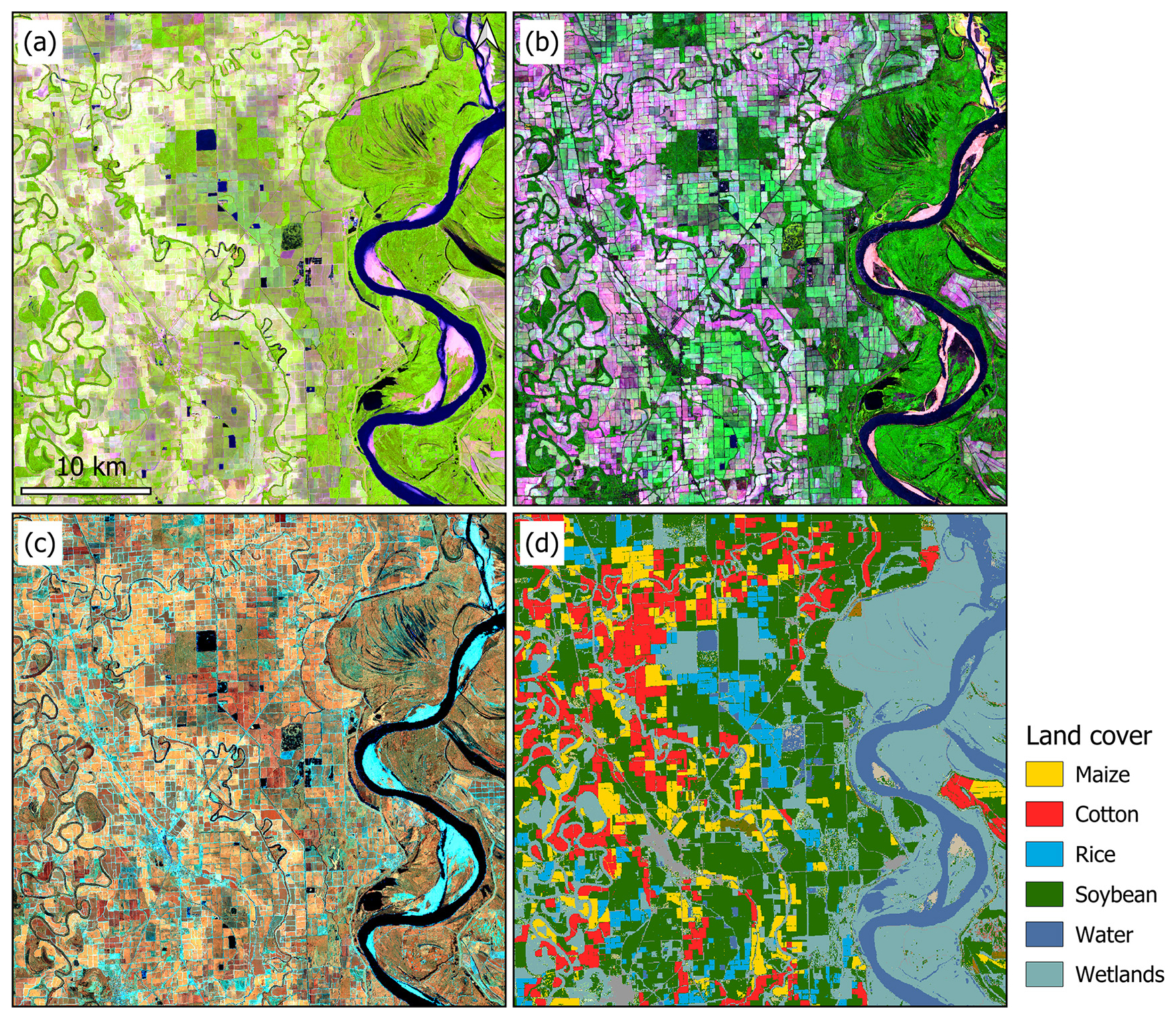
Figure 4 Composites of Sentinel-2 multi-temporal metrics in the Mississippi Valley. (a) SWIR1-NIR-Red composite of NBAR average between the 25th and 75th percentiles from observations ranked by individual bands; (b) SWIR1-NIR-Red composite of NBAR amplitude between the second maximum and the second minimum values; (c) NIR-SWIR1-SWIR2 composites of average NBAR between the 90th percentile and the second maximum values from observations ranked by NDVI; (d) 2022 Cropland Data Layer. The coordinate of the center point is (91.312° W, 33.665° N). All panels are displayed in the same scale at 10 m resolution. Figure contains modified Copernicus Sentinel data (2022).

2.2 Sampling design and field survey

To support the 10 m crop mapping, we conducted extensive field surveys for in situ data collection, based on a two-stage cluster sampling design following Song et al. (2017). This approach has been demonstrated to be effective for agricultural applications in which ground reference data are collected at regional (Khan et al., 2018), national (King et al., 2017; Li et al., 2023), and continental (Song et al., 2021b) scales.

2.2.1 Sampling design

Following previous research, we divided the study area into 20 km × 20 km equal-area blocks and designed the two-stage cluster sampling to target fields to visit. We first derived the per-block maize and soybean area fractions from the previous year's crop map, sorted all blocks from the highest to the lowest fraction, and then stratified the ranked blocks into high, medium and low strata. Following previous studies (King et al., 2017; Song et al., 2017), we selected a simple random sample of blocks from each stratum as the primary sampling units (PSUs) and selected a simple random sample of 10 m × 10 m pixels in each PSU as the secondary sampling units (SSUs) (Fig. 5a) (see Table S2).

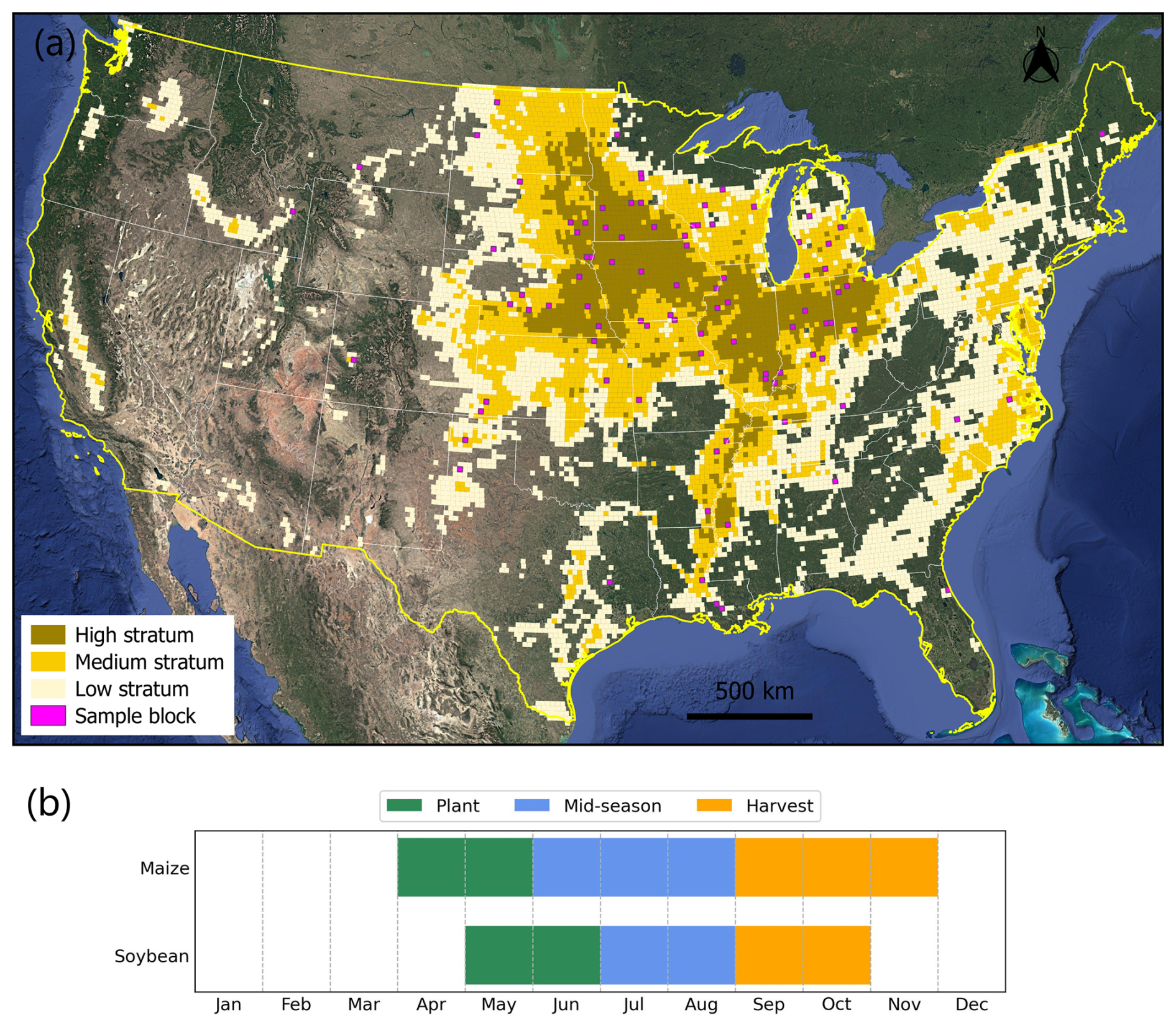
Figure 5 2022 stratified sampling design for field survey. (a) Stratified sampling design. 20 km × 20 km equal-area blocks were stratified into high, medium and low strata. (b) Crop calendar for maize and soybean over the US. Satellite base map is from Imagery © 2025 Landsat/Copernicus, Map data © 2025 Google.

2.2.2 Field data collection

The typical planting season of the US maize starts in April while soybean planting starts in May; the harvesting season starts in September and ends in November for maize and in October for soybean (see Fig. 5b above). We conducted the field survey during the peak growing season in July and August. Consistent with previous research (Li et al., 2023; Song et al., 2021a), we collected two types of datasets during the field survey: (1) ground reference data over the probability sample of SSUs for map evaluation and crop area estimation; and (2) “windshield survey” reference data for model training. These windshield survey data were collected along the driving routes between the SSUs, and were only used to train models for classification and not for validation, whereas the probability sample was exclusively used for validation.

For each year from 2019 to 2022, we selected a separate stratified two-stage cluster sample following the general sampling framework and collected in-season ground data (Fig. 6, Tables S2–S4).

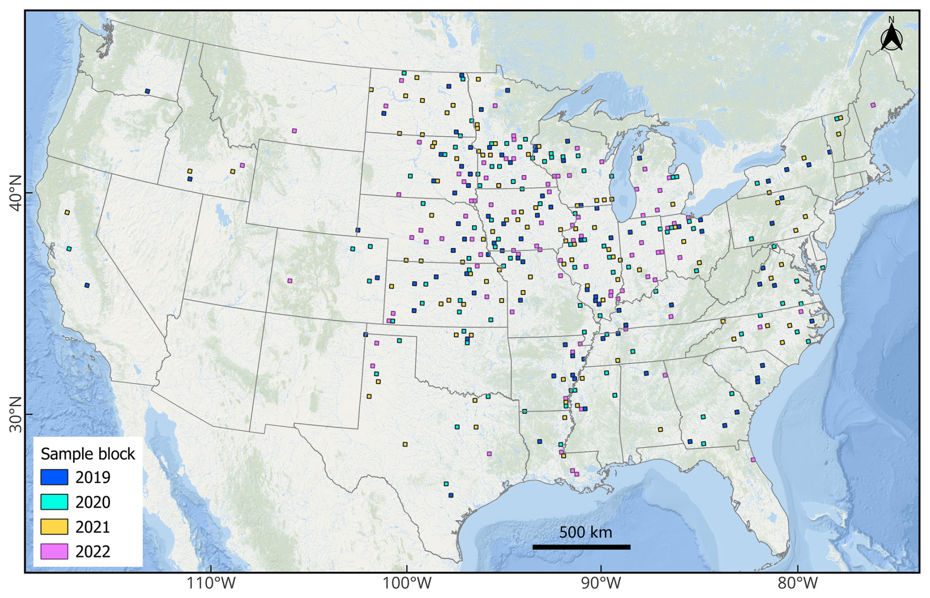
Figure 6 Annual primary sampling unit (PSU) blocks from 2019 to 2022. Background base map source: Esri | Powered by Esri.

2.3 Crop classification

We conducted crop classifications in two stages: (1) at the PSU level, we mapped maize and soybean over all sample PSUs using field data, Sentinel-2 time-series imagery, and decision tree classifiers; and (2) at the national scale, we employed random forest classifiers to map maize and soybean using the PSU-maps as training, multi-temporal metrics derived from Sentinel-2 ARD as well as the topographic features derived from TanDEM-X (DLR, 2015) as input. We evaluated the accuracy of the national crop map using the field data from the SSUs to determine the reference class label.

2.3.1 PSU-level crop mapping

We processed all available Sentinel-2 data over the PSUs from 1 May to 31 October to produce in-season PSU-level maize and soybean maps. For each PSU in each year, we trained two decision tree classifiers separately for maize and soybean classification by using all the bands and normalized ratios of any two bands, as well as the “windshield survey” points as training (Fig. 7b). Applying the trained models to time-series images, we created a binary maize/non-maize map and a binary soybean/non-soybean map at 10 m resolution for each PSU (Fig. 7c). These in-season PSU maps from 2019 to 2022 were then pooled as training labels for national-scale wall-to-wall mapping.

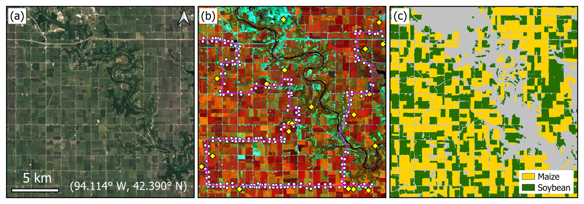
Figure 7 An example of primary sampling unit (PSU) block-level crop mapping using field data. (a) A representative sample block in Illinois with center coordinates shown on Imagery © 2025 Landsat/Copernicus, Map data © 2025 Google. (b) Field data collection in the PSU. The secondary sampling units (SSUs) of pixels are shown as yellow diamonds. The “windshield survey” points are shown as white dots. The driving routes are shown in pink tracks. (c) PSU-level crop maps.

2.3.2 Wall-to-wall crop classification

The multi-temporal metrics derived from the Sentinel-2 ARD were the main input for national mapping. In addition, we downloaded the nominal 12 m TanDEM-X data from the German Aerospace Center (DLR, 2015), and derived 10 m spatial resolution elevation, slope, and aspect using nearest neighbor resampling. These topographic data were combined with the multi-temporal metrics (see Sect. 2.1.4 above) as inputs for supervised classification. We generated training labels from the 10 m maize and soybean PSU maps from 2019 to 2022. We randomly selected 0.2 % of maize (soybean) and 0.8 % of non-maize (non-soybean) pixels from each PSU as training labels. Conflict classification pixels from the binary maize and soybean maps were excluded in the training dataset.

To conduct crop classifications, we employed Random Forest (RF), a widely adopted ensemble machine learning algorithm in remote sensing due to its accuracy, computational efficiency, and robustness to noise (Belgiu and Drăguţ, 2016; Breiman, 2001). Following the approach detailed in Li et al. (2023), we tailored RF binary classifiers separately for maize (RF-Maize) and soybean (RF-Soybean), using the pooled training data from 2019 to 2022. The models were fine-tuned using a random search followed by a grid search (Probst et al., 2019), on a randomly selected subset of 1 % of the training dataset, and subsequently re-trained with optimal hyperparameters on the entire training dataset (see more technical details in Figs. S1, S2 and Table S5 in the Supplement).

We aggregated the per-pixel class probability layers from RF-Maize and RF-Soybean by selecting the highest probability (maize vs. soybean) and derived the aggregated probability layer and corresponding crop mask layer (see Fig. S3 for an example). We then applied a 5 × 5 pixel kernel opening followed by a 10 × 10 pixel kernel closing, to eliminate scattered pixels and fill holes within large homogeneous fields. The kernel sizes were selected based on tests and visual assessments to balance noise removal while preserving fine details. We generated the final maize and soybean map using the aggregated probability layer following the area-matching approach reported by Song et al. (2017, 2021b) and Li et al. (2023).

2.4 Map evaluation

2.4.1 Accuracy assessment

Utilizing the annually field-visited SSUs, we validated the annual maps from 2019 to 2022. Overall accuracy (OA), user's accuracy (UA) and producer's accuracy (PA) with associated uncertainty estimates were estimated using a ratio estimator for two-stage cluster sampling within a stratified design, following good practices (Olofsson et al., 2013; Stehman, 2014). The formulas for accuracy estimation are found in Song et al. (2017, Appendix A)

2.4.2 Crop area comparison with official statistics

We derived the pixel-counting-based crop areas for maize and soybean from the annual crop maps, for each year from 2019 to 2022. We compared these crop areas with the official statistical crop areas from the USDA NASS at the county and state levels. We then calculated root-mean-square-difference (RMSD) and r² between the mapped crop areas and the statistical areas.

3 Results

3.1 Visual assessment

Our 10 m crop map reveals well-known spatial patterns of maize and soybean cultivation in the United States (Fig. 8). The dominant soybean cultivation is shown in the Midwest states, the Great Plains states, the Mississippi Valley and the eastern coast, whereas maize is widely distributed across the country.

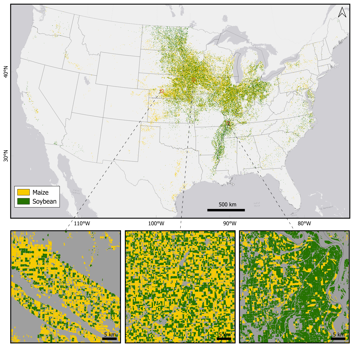
Figure 8 The 10 m maize and soybean map for 2022. Background base map source: Esri | Powered by Esri.

Specifically, our 10 m crop map delineated more field-scale details compared to the 30 m CDL (Fig. 9). Midwest states such as Illinois typically have rectangular crop fields, and our 10 m map generated homogeneous fields with clearer boundaries (Fig. 9a). Our map also captured more landscape fragmentation, such as smaller fields with greater crop diversity in the Mississippi Valley (Fig. 9b) and the agriculture/wetland mosaic in North Dakota (Fig. 9c).

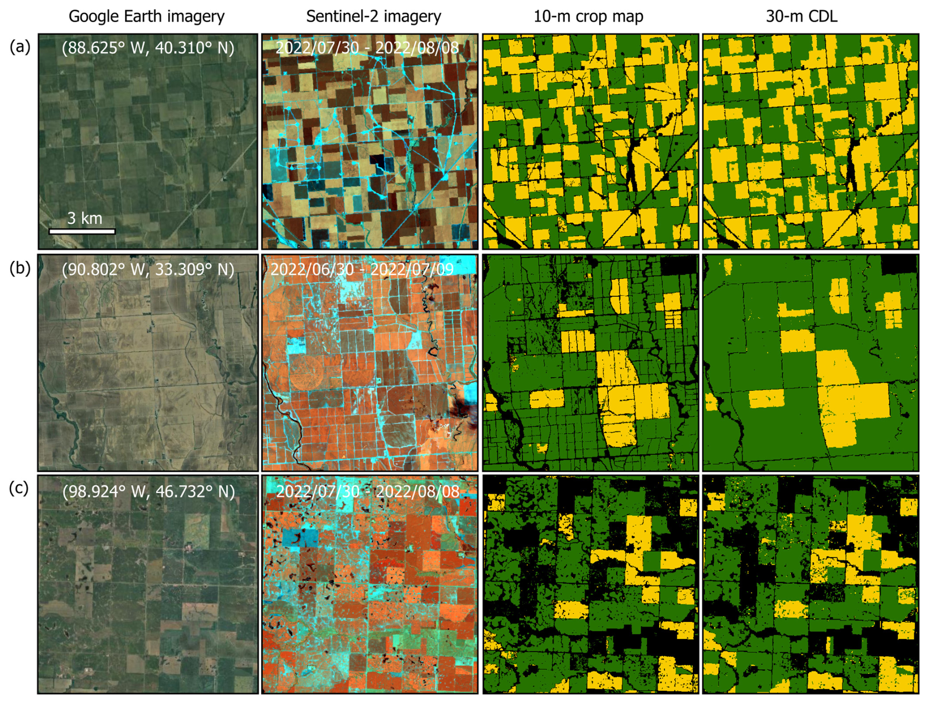
Figure 9 Maize and soybean classification in 2022 over selected regions. Rows (a)–(c) are representative sites in Illinois, Mississippi, and North Dakota. All panels are displayed at the same scale (10 km × 10 km). The coordinates of the center points are shown on Imagery © 2025 Landsat/Copernicus, Map data © 2025 Google. The 10 d composite periods are shown on the Sentinenl-2 image (R: NIR, G: SWIR1, B: SWIR2). Maize and soybean are shown in yellow and green colors, respectively.

3.2 Quantitative accuracy assessment

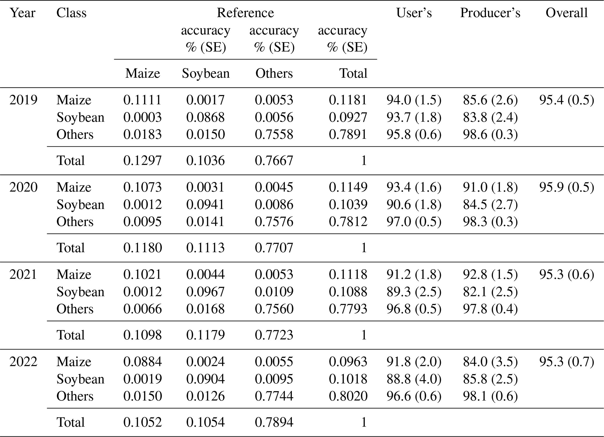
We conducted an accuracy assessment for annul maps using the annual SSUs as references (Table 1). All maps achieved OAs greater than 95 % with standard errors less than 1 %. UAs and PAs for maize were higher than 91 % and 84 %, respectively, while UAs and PAs for soybean were higher than 89 % and 82 %, respectively.

Table 1 Accuracy assessment for maize and soybean maps from 2019 to 2022. Cell entries in the confusion matrices represent area proportions. Reference data were derived from probability samples of secondary sampling units (SSUs).

3.3 Comparison between the crop maps and agricultural statistics

We compared our map-based area estimates with agricultural statistics reported by the NASS at state and county scales. The state-level area comparisons between our mapped areas and the NASS statistics showed close agreements, with r² greater than 0.99 and root-mean-square-difference (RMSDs) less than 900 km² for maize, and RMSDs less than 1800 km² for soybean (Fig. 10). At the county level (Fig. 11), our mapped maize and soybean areas also matched the NASS statistics well with r² greater than 0.97 and RMSDs between 30 and 50 km².

Figure 10 State-level comparison between mapped maize and soybean areas and NASS statistics.

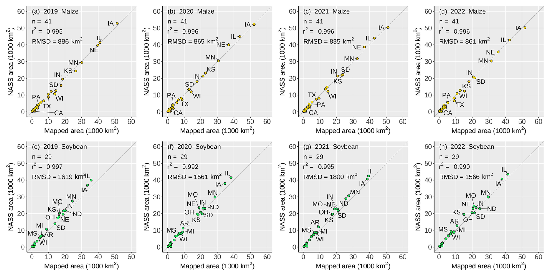
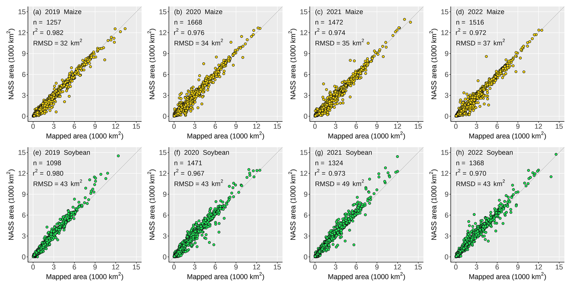
Figure 11 County-level comparisons between mapped maize and soybean areas and NASS statistics.

4 Discussion

4.1 The benefits of 10 m crop maps in mixed pixel reduction

Using the 2022 10 m crop map as an example, we conducted a quantitative data analysis to illustrate the benefits of 10 m crop mapping over 30 m mapping. We first removed small fields less than nine 10 m pixels (one 30 m pixel), then spatially aggregated the 10 m map to 30 m resolution and derived the maize and soybean cover fraction for each 30 m pixel. We defined pure pixels as 100 % cover and anything below as mixed pixels. We applied a 50 % cover threshold to determine the dominant crop type within mixed pixels. Pixels where neither maize nor soybean cover reached 50 % were ignored. Rather than assessing accuracies for the aggregated 30 m maps, our objective was to compare the 10 m versus 30 m resolution by quantifying changes in mixed pixels and analyzing the spatial patterns.

Unsurprisingly, the aggregated 30 m map showed that pure pixels are clustered in large-size homogeneous fields (Fig. 12a). Mixed pixels occurred in small, fragmented fields, on field edges, or along the road networks, where crops coexisted with other land cover (e.g., other crops, pasture, built-up, etc.) (Fig. 12b, c). Our 10 m maps showed clear advantages over the 30 m CDL in mixed pixel reduction in various landscapes (Fig. 13). In North Dakota where numerous fields are fragmented, the 10 m map presents more homogeneous fields and captures within-field patterns of water ponds (Fig. 13a); for center-pivot irrigated fields in Nebraska, the 10 m map delineates cleaner circular patterns (Fig. 13b); in Appalachian Pennsylvania where many fields are in narrow strips, the 10 m map distinguishes neighboring strip cropping fields better than the 30 m CDL in which the fields are mapped with a large amount of mixed pixels (Fig. 13c).

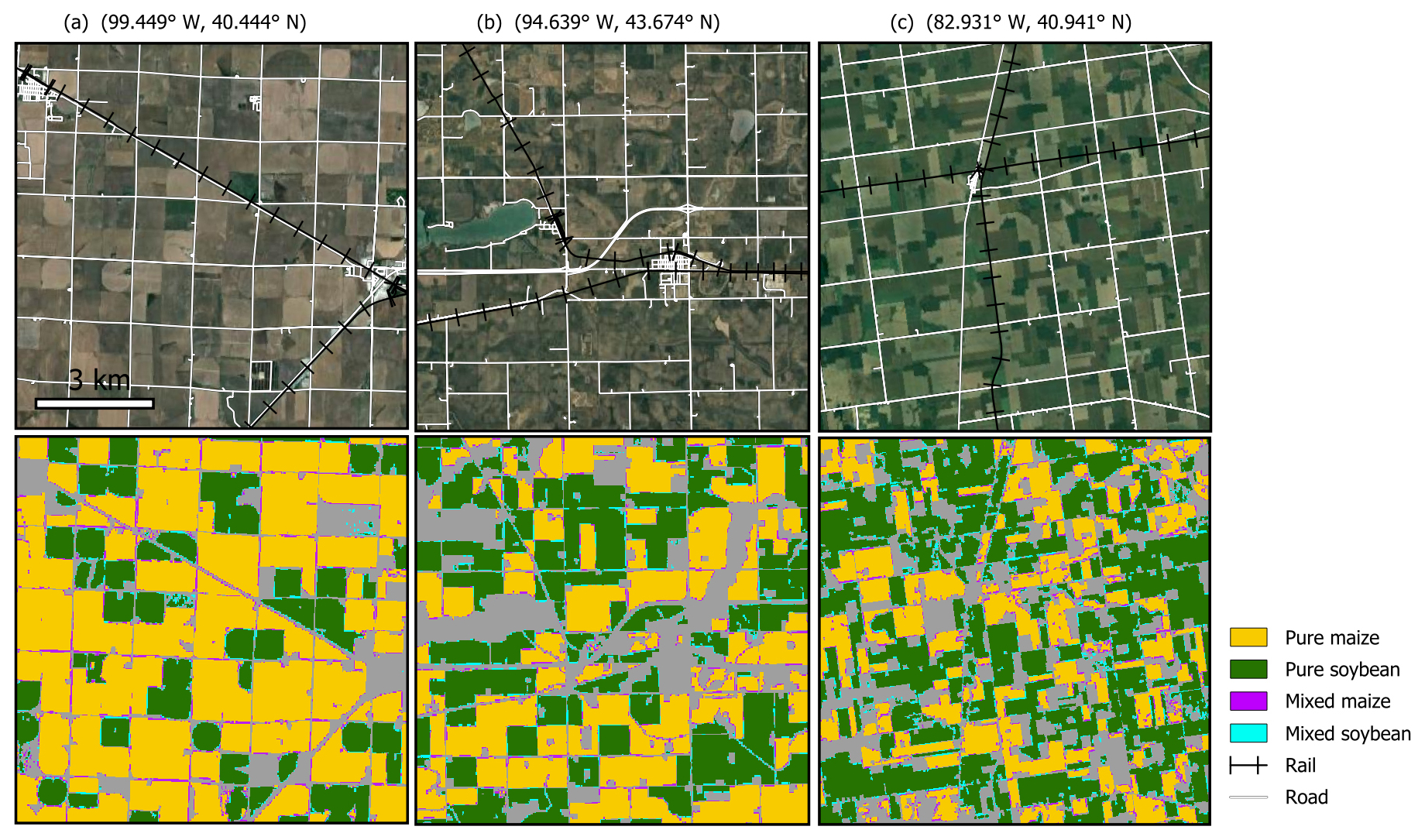
Figure 12 The 2022 aggregated 30 m maize and soybean map overlaid with road and rail networks. Columns (a)–(c) are selected sites in Nebraska, Minnesota, and Ohio. The 30 m map was derived by spatially aggregating the 10 m map by calculating the fractional cover and categorized as pure pixels with 100 % cover or mixed pixels with <100 % cover. All panels are displayed at the same scale (10 km × 10 km). The coordinates of the center points are shown on Imagery © 2025 Landsat/Copernicus, Map data © 2025 Google. The rail and road networks are obtained from the US TIGER database.

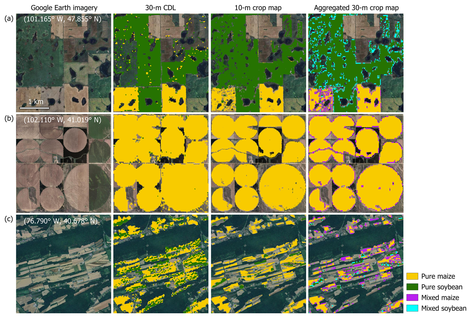
Figure 13 The 2022 aggregated 30 m maize and soybean map and CDL show mixed pixels in various landscapes. (a) Wetland/agriculture mosaics in North Dakota; (b) center-pivot irrigated fields in Nebraska; (c) strip fields in Pennsylvania. The coordinates of the center points are shown on Imagery © 2025 Landsat/Copernicus, Map data © 2025 Google.

We obtained the percentage of mixed maize and soybean pixels at the county level to examine the spatial distribution of mixed pixel reduction from 30 to 10 m (Fig. 14). The counties with the highest maize and soybean production, such as those in Iowa, Illinois, and Nebraska, had the least mixed pixel percentages ranging from 1 % to 10 %, while counties in the upper Midwest, the North and South Plains, the northeast and eastern coast had more mixed pixels (Fig. 14a, c). Overall, the median percentages of mixed maize and soybean pixels in all counties were 8 % and 9 %, respectively (Fig. 14b, d). Our results show that increasing the spatial resolution of crop mapping from 30 to 10 m would reduce the number of mixed pixels by 8 %–9 % at the county scale, and substantially benefit many states outside of the Midwest region.

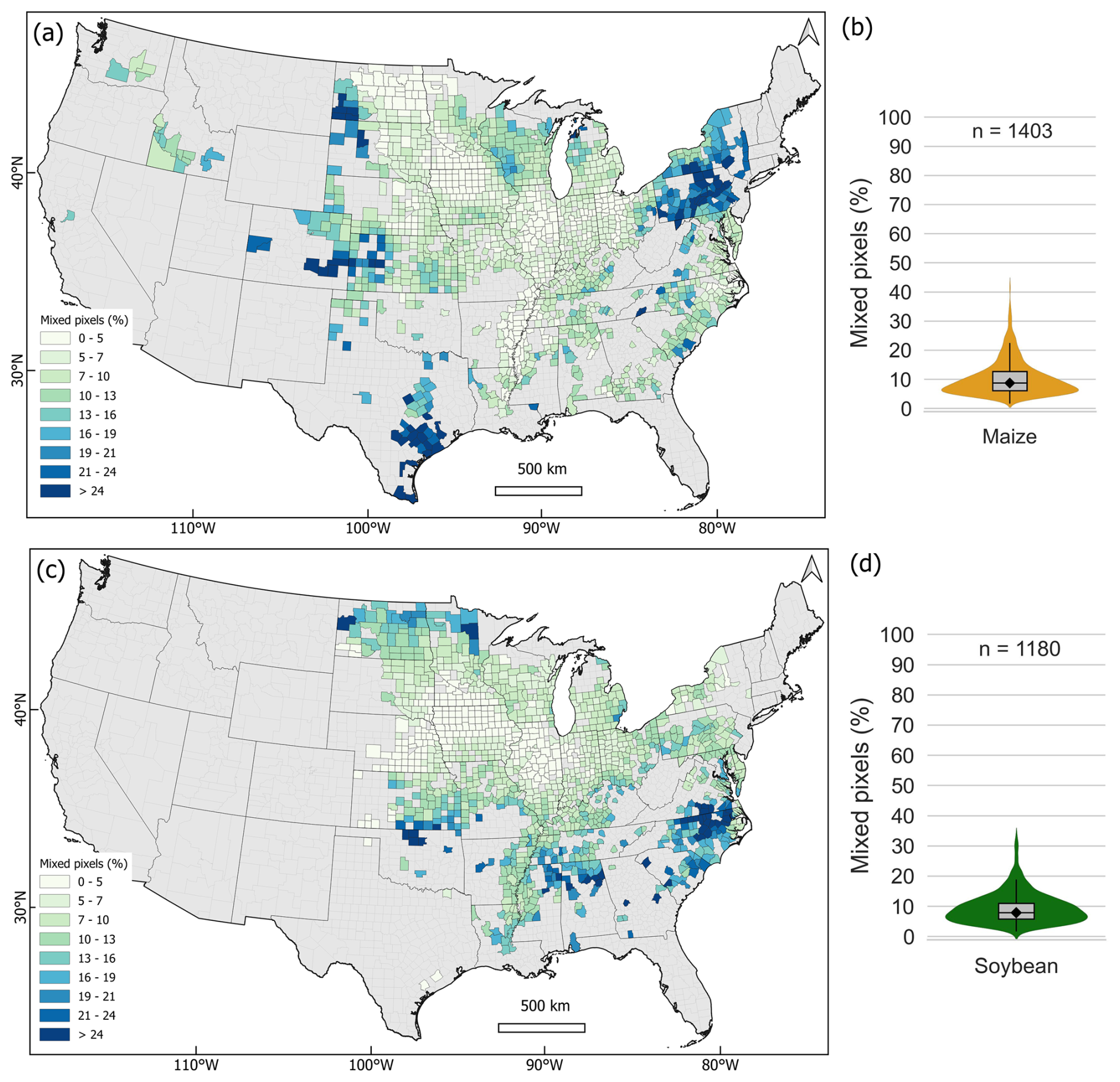
Figure 14 The percentages of 30 m mixed maize and soybean pixels at the county level derived from the 10 m map. (a) The spatial distribution of mixed maize pixels; (b) the statistical distribution of mixed maize pixels; (c–d) the same as (a)–(b) but for soybean. Counties accounting for 99.9 % coverage of the national maize and soybean cultivation derived from the 2022 NASS statistics are shown.

We conducted additional analysis by comparing our aggregated 30 m map with the 30 m CDL for the maize and soybean classes. We applied a 50 % threshold to convert our aggregated 30 m map to binary maize and soybean maps and conducted a per-pixel comparison. We then aggregated the per-pixel results to the county level based on the ratio of the difference of maize or soybean pixels between our map and CDL divided by maize or soybean pixels in CDL. Positive values indicate more maize or soybean pixels in our map, whereas negative values indicate more pixels in CDL (Fig. 15). In several regions, our map presented more maize pixels, such as in northern Texas and southern Louisiana (Fig. 15a), and more soybean pixels, such as in western North Dakota and Georgia (Fig. 15c). In general, CDL reported more maize and soybean pixels in most counties compared to our aggregated 30 m map (Fig. 15b, d), which is likely due to the exclusion of 10 m maize and soybean pixels below the 50 % threshold during aggregation.

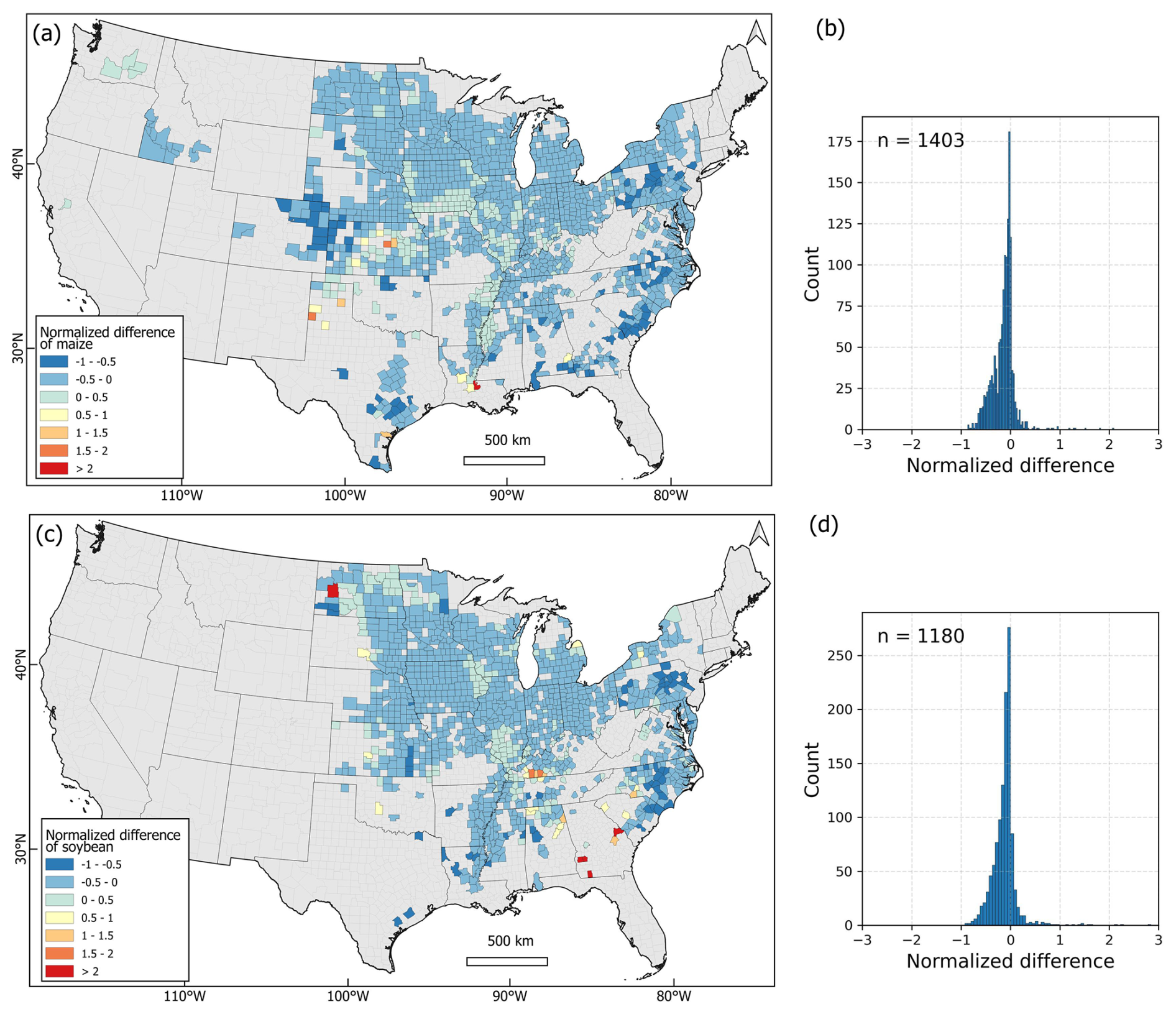
Figure 15 Comparison between our aggregated 30 m map with the 2022 30 m CDL at the county level. (a) Normalized difference of maize pixel; (b) histogram of the normalized difference of maize pixel; (c–d) the same as (a)–(b) but for soybean. Counties accounting for 99.9 % coverage of the national maize and soybean cultivation derived from the 2022 NASS statistics are shown.

To estimate the number of mixed pixels that might be reduced by improving the CDL's spatial resolution from 30 to 10 m, we overlaid the 2022 30 m CDL on our 30 m fractional cover map, and computed the number and proportion of CDL maize and soybean pixels that were mixed pixels at the county level (Fig. 16). The mixed pixel derived from CDL showed similar spatial distribution patterns to results derived from the aggregated 30 m map (see Fig. 14 above). The median percentage of mixed pixels across all counties for both maize and soybean was 8 % (Fig. 16b, d), which is close to the values of 8 % (9 % for soybean) derived from our aggregated 30 m map (see Fig. 14 above). These consistent mixed pixel estimates from our map and the CDL indicate substantial benefits of 10 m crop maps in reducing mixed pixels over existing 30 m products, especially for regions outside of Midwest, as illustrated in our analyses.

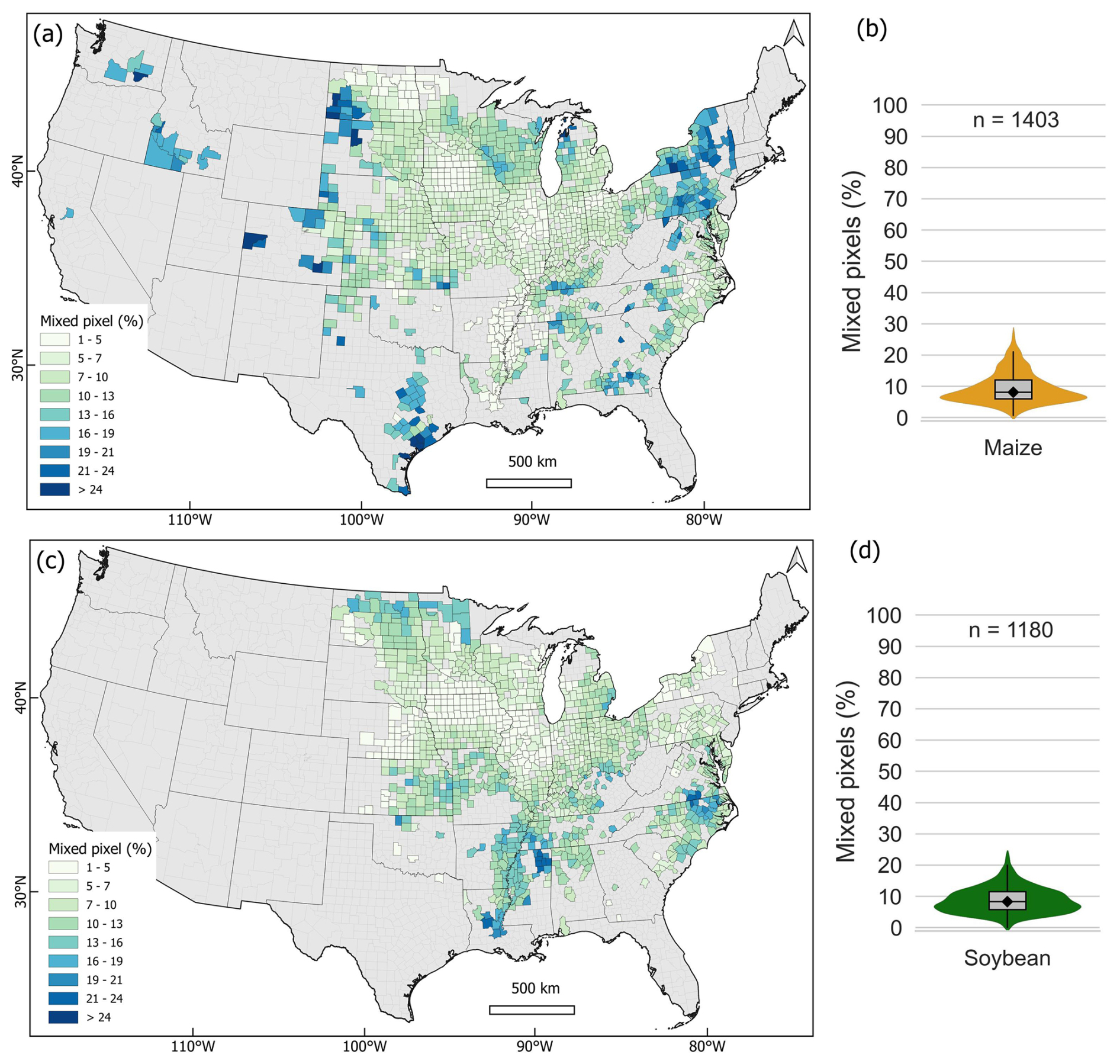
Figure 16 The percentages of 30 m mixed maize and soybean pixels at the county level by comparing our aggregated 30 m map and the 2022 30 m CDL. (a) The spatial distribution of mixed maize pixels; (b) the statistical distribution of mixed maize pixels; (c–d) the same as (a)–(b) but for soybean. Counties accounting for 99.9 % coverage of the national maize and soybean cultivation derived from the 2022 NASS statistics are shown.

4.2 The potential of 10 m crop maps in finer-scale agricultural monitoring

Higher-resolution crop maps have great potential to facilitate remote-sensing-based agricultural applications at finer scales. For example, the Crop Sequence Boundaries (CSB), which delineate polygons of homogeneous cropping sequences with 8-year moving windows, have been developed based on the CDL by the USDA (Hunt et al., 2023). The 30 m CDL was resampled to 10 m resolution to improve the masking of road networks as the roads and rails in rural areas are typically less than 30 m in width. Consequently, the resampled 10 m maps may delineate inaccurate field boundaries due to mixed pixels (Fig. 17). The CSB delineated large homogeneous fields well (Fig. 17a) but showed more fragments when encountering within-field cropping variations (Fig. 17b). The misalignments between the delineated field edges and pixel boundaries are extensive in heterogeneous landscapes and small fields (Fig. 17c, d), and thus the polygon-based crop acreage derived from CSB layers may be biased. Alternatively, using originally produced higher-resolution (e.g., 10 m) maps can yield more accurate field delineation, cropping sequences, and crop area estimates with smaller uncertainties (Duveiller and Defourny, 2010; Ozdogan and Woodcock, 2006; Yan and Roy, 2014).

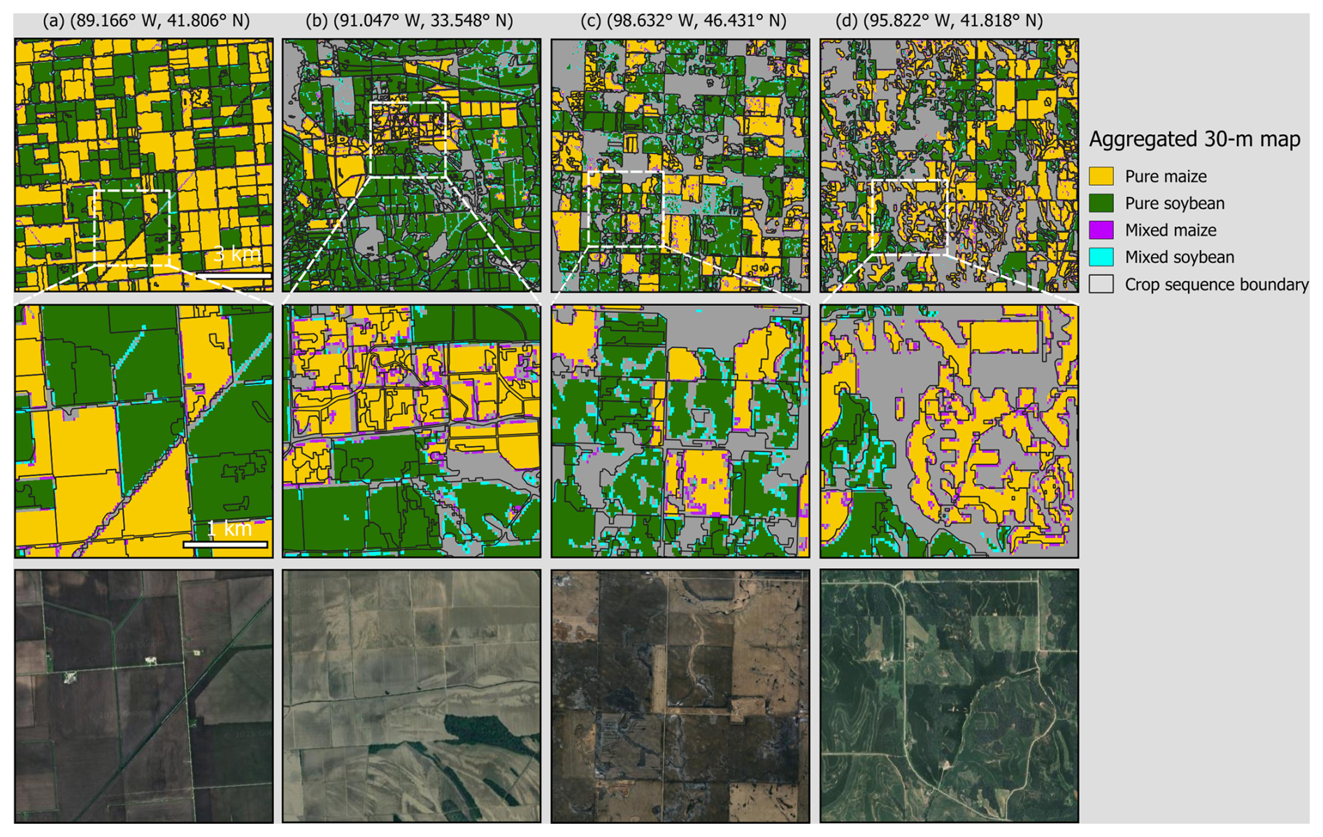
Figure 17 The aggregated 30 m maize and soybean map overlaid with Crop Sequence Boundaries. Columns (a)–(d) are selected sites in Illinois, Mississippi, North Dakota, and Iowa. All panels are displayed at the same scale (10 km × 10 km). The coordinates of the center points are shown. The 2015–2022 Crop Sequence Boundaries are obtained from the USDA NASS. Satellite base map is from Imagery © 2025 Landsat/Copernicus, Map data © 2025 Google.

With higher-resolution satellite imagery available from continuous observations (e.g., Sentinel-1 and Sentinel-2) and upcoming missions (e.g., Landsat Next, NASA-ISRO SAR Mission (NISAR)), we anticipate that 10 m crop maps will play a more critical role in agricultural monitoring from the field to global scales.

4.3 The robustness of temporal metrics for annual crop map production

Stacking satellite-derived time-series maps is one of the most common practices to investigate long-term agriculture-related land cover and land use change, such as cropping history (Blickensdörfer et al., 2022; Johnson, 2019), crop and cropland expansion (Lark et al., 2020; Potapov et al., 2021a; Song et al., 2021b; Zalles et al., 2019), and cropland intensification (Kehoe et al., 2017; Marin et al., 2022). However, in large-extent countries such as the US, the spatiotemporal consistency in multi-year crop classifications can be impacted by both intra-annual and interannual variations in crop phenology (Fig. 18). For example, the 2022 NDVI time series for maize and soybean showed noticeably different crop progress across the CONUS (Fig. 18a, b). In Arkansas, maize growth peaked in mid-May and started senescence in early August, whereas maize in the Midwest states was at early growing stages in mid-May and at the peak growing season in early August. Soybean also showed noticeable disparities in crop progress across the US states. On the other hand, interannual phenological shifts also impede the classification consistency (Fig. 18c, d). In Illinois, similar NDVI profiles between 2020 and 2022 suggested overall consistent growing progress, while the patterns in 2019 and 2021 showed higher interannual variations. In 2021, Illinois experienced an earlier planting pace for maize and soybean partly due to the favorable spring weather conditions and soybean varieties adapted to early plantation (Nafziger, 2024). In 2019, crop phenology shifted substantially as a result of planting delays caused by extremely heavy precipitation in the spring (Manoochehr et al., 2021). Consequently, at the state level in Illinois, maize was planted at only 24 % compared to the previous year's 95 % and the five-year average of 49 % by the end of May 2019; soybean was planted at 9 % compared to the previous year's 79 % and the five-year average of 51 % (NASS CPR, 2024).

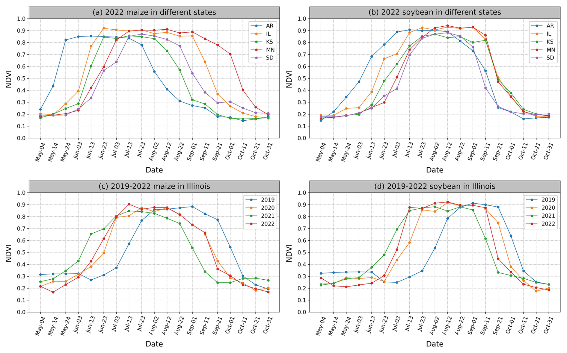
Figure 18 NDVI time series for maize and soybean from representative sites. (a) 2022 maize NDVI in Arkansas (AR), Illinois (IL), Kansas (KS), Minnesota (MN), South Dakota (SD); (b) the same as (a) but for soybean; (c) 2019–2022 interannual NDVI variations for maize in Illinois; (d) the same as (c) but for soybean. The details about the sites are shown in Fig. S4 and Table S6.

Utilizing the multi-temporal metrics to relatively normalize crop phenological variations, our approach can be applied to generate annual crop maps over large areas, as also illustrated for South America in Song et al. (2021b). Our four-year sampling designs generated large field samples, allowing us to collect representative training data from various growing conditions and geographical regions. Our workflow generated consistently accurate maize and soybean maps over the entire CONUS, from 2019 to 2022. The map accuracies for 2019 (an abnormally wet year), and 2020 and 2021 (both years with normal weather) are consistent with those of 2022 (see Table 1 above).

5 Data availability

The annual 10 m maize and soybean maps over the CONUS from 2019 to 2022 are openly accessible at the website of the Global Land Analysis and Discovery (GLAD) team at the University of Maryland (https://glad.umd.edu/dataset/mapping-crops-10-m-resolution-united-states, last access: 26 December 2025). The dataset is also available at https://doi.org/10.6084/m9.figshare.28934993.v2 (Li et al., 2025). The dataset includes a set of GeoTIFF images in the ESPG:4236 spatial reference system. The values 0, 1, 2, 255 represent other, maize, soybean, and no data, respectively. External data used in this study are openly accessible online: (1) the Sentinel-2 data were downloaded from Google Cloud Platform (https://console.cloud.google.com/marketplace/product/esa-public-data/sentinel2?project=s2data Google Cloud Console, 2025); (2) the Cropland Data Layer were downloaded from the US Department of Agriculture (USDA) National Agricultural Statistics Service (NASS) (https://www.nass.usda.gov/Research_and_Science/Cropland/Release/index.php, NASS CDL, 2025; (3) the TanDEM-X was downloaded from the German Aerospace Center (https://tandemx-science.dlr.de/, DLR, 2015); (4) the agricultural statistics for CONUS were retrieved from the USDA NASS (https://www.nass.usda.gov/Quick_Stats/, USDA NASS, 2025); (5) the Crop Sequence Boundaries were derived from the USDA NASS (https://www.nass.usda.gov/Research_and_Science/Crop-Sequence-Boundaries/index.php, NASS CSB, 2024); (6) the road and rail networks were downloaded from the US TIGER database (https://www.census.gov/geographies/mapping-files/time-series/geo/tiger-line-file.html, US Census Bureau, 2025).

6 Conclusions

Crop maps at 10 m spatial resolution bring substantial benefits for agricultural applications compared to 30 m products for smallholder as well as industrial agricultural countries. In this study, we developed 10 m maize and soybean maps over the Contiguous US (CONUS) from 2019 to 2022, using all available Sentinel-2 observations and field surveys, with overall accuracies consistently greater than 95 %. We explicitly examined the benefits of improving the spatial resolution from 30 to 10 m by quantifying the reduction in mixed pixels. Our analysis showed that, across all counties in the US, the 10 m maps reduced mixed pixels by a median of 8 % for maize and 9 % for soybean compared to the aggregated 30 m maps, with most mixed pixels occurring along field edges, road networks, and in heterogeneous fields. Our workflow generated annual maps with consistency across space and over time. Our 10 m crop maps were produced at the end of the growing season, around 3–4 months earlier than the official 30 m Cropland Data Layer. As more Sentinel-2-like data become accessible from current observations and planned missions such as Landsat Next, 10 m crop maps presented in this study will greatly benefit agricultural applications, including field boundary extraction, crop sequence delineation, crop condition monitoring, precision fertilization and irrigation, from field to global scales.