The Loobos ecosystem first tower dataset: meteorology, turbulent fluxes and net ecosystem exchange (1996 to 2021)

We describe a 25 years (1996–2021) observational dataset of meteorology, turbulent fluxes and net ecosystem exchange collected from the first tower at the Loobos site, the Netherlands (NL). This is one of the 17 first FLUXNET sites globally. The presented dataset contains six data streams, namely (1) the NL-Loo_BM stream including meteorological data: four-component radiation (radiation balance), air temperature and relative humidity, wind information, precipitation and throughfall, photosynthetic active radiation, bole temperature and soil heat flux), (2) the NL-Loo_Profile stream containing vertical profiles of CO₂ mole fraction, H₂O pressure, air temperature and relative humidity, (3) the NL-Loo_ST stream derived from the aforementioned two streams including total stored heat flux, H₂O and CO₂ fluxes below the canopy, (4) the NL-Loo_EC stream including EC measurements of CO₂ flux, sensible heat and latent heat fluxes, (5) the NL-Loo_Soil stream including vertical profiles of soil moisture and temperature and ground water level data, and (6) ancillary data including soil respiration, vegetation properties (i.e., tree height, stem width and dry aboveground biomass, Leaf Area Index, sap flow, needle foliage properties and the associated nutrient analysis) and ground water level. The data quality of these data streams is assured through standard operating procedures. To show the utility of gathering long-term and comprehensive measurements, we present analyses of mean diurnal storage CO₂ flux, the trend of NEE over the last 25 years and the energy balance closure. Being one of the longest datasets of its kind in a temperate forest, this valuable dataset is anticipated to be used for investigating the performance of various gap-filling algorithms, semi-climatological trends including extreme climatic events (such as the heatwave of 2003 and the drought of 2018) and the role of forest ecosystem in the carbon, water and energy cycle. Meanwhile, it is expected to be employed for validating modelled land-atmosphere CO₂ and turbulent exchange fluxes, verifying model assumptions and serving as ground truth for satellite data retrievals. The dataset is accessible at https://doi.org/10.5281/zenodo.15721310 (Zhao et al., 2025) under a CC-BY4 open use license, where it is published as an associated station-like site and the same data will also be available at the European Fluxes Database Cluster. Hence, the data will be committed to the FLUXNET Data System Initiative too. It is noted that in 2021 a second tower was built and equipped with new instrumentation as a replacement of the first tower, which was labelled as an ICOS Ecosystem Class 2 site in 2023. Here we describe the first tower's instrumentation and data processing up to a Level 1 product (derived variables and quality checks, but not gap-filled). The instrumentation and data processing related to the second tower is described in van der Molen et al. (2026).

1 Introduction

In 1995, a tower was built in the Loobos forest area in the Netherlands to measure water, heat and momentum fluxes for investigating forest evapotranspiration using the eddy covariance method (referred to as EC from here on) (Dolman et al., 1998). Following the Kyoto negotiations, which sought to operationalize the United Nations Framework Convention on Climate Change by committing industrialized countries and economies in transition to limit and reduce greenhouse gas emissions (https://unfccc.int/kyoto_protocol, last access: 15 December 2024) One of the key questions raised by the Kyoto Protocol was how to calculate the changes in carbon stocks associated with land use changes and forestry activity (IGBP Terrestrial Carbon Working Group, 1998). This required to also observe the carbon dioxide (CO₂) balance for forest ecosystems (Valentini et al., 2000). Consequently, since 1996, CO₂ flux measurements have been conducted in Loobos, which subsequently became one of the 17 first FLUXNET sites globally (https://fluxnet.org/data/la-thuile-dataset/lathuile-data-summary/, last access: 15 December 2024).

The Loobos site is located near Kootwijk ($\mathrm{52}\mathit{°}{\mathrm{9}}^{\prime }{\mathrm{59.50}}^{\prime \prime }$ N–$\mathrm{5}\mathit{°}{\mathrm{44}}^{\prime }{\mathrm{36.99}}^{\prime \prime }$ E). A 22 m tall tower was built on a small dune (please refer to photos of Fig. A1 in Appendix A1). The tower base is at 26.4 m above mean sea level (Fig. 1). The main tree species is Scots pine (Pinus sylvestris). In all directions the forest extends for more than 1.5 km. The forest was planted around 1911 on bare sand (Kadaster, 2025) to control the drifting of the sand and provide wood for the mining industry. Before planting, sand dunes had formed with heights between 2 and 10 m relative to the valleys in between. The trees are now widely spaced with some open spots. In a radius of 500 m around the flux tower 89 % of the area is covered with Scots pine (Pinus sylvestris), 3.3 % with Corsican or black pine, 2.3 % with birch, 1.3 % with Douglas fir, 0.6 % with oak (Quercus Robur) and 3.5 % of the area is open and mostly covered with heather and grass (Moors, 2012). The average tree height increased from 15.3 m in 1996 to 20.6 m in 2020, with a mean annual growth rate of 0.22 m. Trees on top of dunes tend to be shorter than trees growing in the valleys, hence the local topography is not visible from above the canopy. The undergrowth of the forest has exhibited a notable increase in coverage over time, particularly since 1976. It consists of mosses (Polytrichum spp.), grasses (Deschampsia flexuosa), blueberries (Vaccinium myrtilus), and shrubs (dominated by American cherry of Prunus serotina and Amelanchier lamarckii) (Moors, 2012) (please refer to photos in Appendix A1). It is noteworthy that at the outset of the observation period, Vaccinium was absent, yet it now constitutes the majority of shrubs, indicating a notable increase in its spread over time (please refer to photos in Appendix A1). Because of the local topography caused by the sand dunes, the distance to the ground water table depends on the location. In the valleys, the ground water table is at a depth ranging from 2.5 to 4.3 m below the surface. More details on the soil and vegetation composition in the first period of the site can be found in the report by Moors (2012).

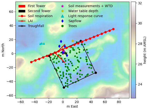
Figure 1 A map of measurement locations at the Loobos first tower. The first tower is in the center (0,0) m. The black square delineates the area where the tree inventories were done in 2000, 2005, 2008, 2012 and 2025. The green dots show the locations of the trees in the inventory.

Measurement locations at the Loobos first tower site are mapped in Fig. 1. The collected dataset contains measurements of meteorological variables (e.g., radiation components, precipitation, vertical profiles of wind, air temperature, humidity and CO₂, soil temperature and moisture content), turbulent fluxes (i.e., latent heat and sensible heat and CO₂) at half-hourly intervals. The dataset from the first tower has been used in many national and international studies and has been cited more than 150 times in peer-reviewed articles, including papers in high impact journals like Nature (Keenan et al., 2013; Valentini et al., 2000; Enquist et al., 2003). The conducted studies range from: (1) the development of data quality control and gap-filling strategies for long term energy flux datasets (Falge et al., 2001a, b; Reichstein et al., 2005; Pastorello et al., 2020; Meesters et al., 2012; Göckede et al., 2008), (2) data analysis including trend analysis (Dolman et al., 2002; Falge et al., 2002; Tong et al., 2023; Elbers et al., 2011) and to study the response of the ecosystem to droughts, heat waves and warm winters (Lansu et al., 2020; van der Horst et al., 2019; Granier et al., 2007; Zhou et al., 2024; Mallick et al., 2024; García-García et al., 2023; Vermeulen et al., 2015), (3) analyses of carbon and water fluxes exchange dynamics via model development and validation studies (Kramer et al., 2002; Veroustraete et al., 2002; Falge et al., 2003; Papale and Valentini, 2003; Hari et al., 2018; Aubinet et al., 1999; Wu et al., 2020; Strebel et al., 2024; Vermeulen et al., 2015), (4) the development of land surface models and parameter optimizations (Chen et al., 2016; Raoult et al., 2016; Harper et al., 2016; Largeron et al., 2018), (5) the development of the CarboEurope regional experiment strategy (Dolman et al., 2006), (6) ecological and land management studies (Van Wijk and Bouten, 1999; Dolman et al., 2003; Ceulemans et al., 2003; Balzarolo et al., 2016; Churkina et al., 2003; Jansen et al., 2023; George et al., 2021), (7) serving as ground truth for satellite data retrievals such as evapotranspiration (Verstraeten et al., 2005; Hu et al., 2017; Petropoulos, 2024) and gross primary productivity (Verma et al., 2014; Joiner et al., 2014), and (8) groundwater management (Moors, 2012).

While the tower and its associated dataset were described in a limited manner (Dolman et al., 2002; Elbers et al., 2011), the purpose of this paper is to provide a comprehensive overview of the instrumentation, data processing and the resulting data archive, enabling its use in data analysis studies, model development and validation of satellite data retrievals. Section 2 describes the instrumentation, basic data processing, data quality control and obtained data records. Section 3 shows data evaluations by presenting data cross-check results, the mean diurnal storage flux in comparison to EC measured fluxes and total fluxes, seasonal and interannual variations in net ecosystem exchange of CO₂ flux and energy balance residual. Section 4 provides conclusions and information on data and code accessibilities.

2 Instrumentation and data processing

2.1 In situ measurements

2.1.1 Meteorological variables

At the top of the scaffolding tower (highest platform at 22 m), standard meteorological measurements were conducted, including air temperature, relative humidity, horizontal wind speed and wind direction. Air pressure was measured at the site at 15 m height starting from February 1999. The four radiation components were measured individually: incoming and reflected shortwave (solar) radiation using two pyranometers, and incoming and emitted longwave (thermal infrared) radiation using two pyrgeometer equipped with a ventilated sensor to ensure reliable readings, particularly during dew and frost events. Additionally, quantum sensors were installed on 9 August 2001 to measure direct photosynthetically active radiation (PAR), diffuse PAR and reflected PAR. These data were sampled every 20 s and stored as half hourly means and standard deviations.

Precipitation was measured using tipping bucket rain gauges with a resolution of approximately 0.2 mm per tip. One rain gauge was located on top of the tower. Another rain gauge was installed in an open space nearby to minimize the error due to high wind. However, this open space measurement was discontinued after 9 January 2007 due to the regrowth of pine trees, which caused the area to no longer be open enough. Throughfall was measured from 2 June 1995 until 23 July 2014 using 36 manual gauges as well as a custom made tipping bucket rain gauge at the end of an approximately 10 m long gutter through with a width of 10 cm. The manual gauges were set up at a 4 m distance from each other in a fixed square of 400 m². The area around these manual gauges was kept free of grass and shrubs. The resolution of the tipping bucket gauge used for the throughfall trough is approximately 0.07 mm per tip depending on the exact surface of the gutter and the precipitation density. This tipping bucket, along with the one on top of the tower, was initially logged at a 5 min intervals, with the tips accumulated over each interval. Since 16 June 2004, a Campbell logger has been recording data at 30 min intervals. Detailed information about the instruments, their manufacturers and their specific locations on the tower is provided in Table 1.

Table 1 List of instruments, installation height and measurement period.

Notably, the key instruments that operate continuously over long periods, such as pyranometers, Vaisala instruments and quantum sensors were maintained on a bi-weekly scale to ensure high-quality and reliable data. Routine maintenance includes visual inspection, cleaning of sensor domes and diffusers of remote dust and other deposits and verification of sensor leveling and alignment.

While these manual interventions ensured optical and structural integrity, the long-term consistency of the data was further supported by the high intrinsic stability of the sensors themselves. For instance, air temperature measurements through Vaisala remained highly stable due to inherent resistance to calibration drift from the platinum resistance thermometers (PT100). Similarly, soil moisture and temperature sensors (Campbell Scientific, Inc.) described in Sect. 2.1.4 demonstrated high temporal stability with negligible sensor drift throughout the study period. While the Vaisala humidity sensors drifted, unfortunately, they were not often calibrated.

The sonic anemometers and wind vanes were characterized by high long-term stability, as their measurement accuracy is dependent on fixed transducer geometry rather than electronic calibration. Any potential measurement deviations were attributed to frame-induced flow distortions rather than transducer degradation; therefore, the anemometer did not require factory calibration.

Radiation sensors were subject to slow, systematic sensitivity degradation due to the environmental aging of the sensor's optical surfaces. To account for this, these instruments were returned for factory recalibration every couple of years. To assess the potential for long-term sensitivity degradation in the radiation measurements, an intercomparison was conducted during an overlapping period (from 21 January 20221 to 29 May 2023). Incoming shortwave radiation in the first tower was compared against a second, independent sensor (Kipp & Zonen) deployed in the second tower (https://meta.icos-cp.eu/resources/stations/ES_NL-Loo, last acces: 11 March 2026, van der Molen et al., 2026). The comparison result demonstrates high instrumental consistency, with relative differences remaining within 5 % when averaged over a weekly time window (Fig. S1 in the Supplement). As such, the calibration drift was not applied in the data processing.

2.1.2 Eddy covariance

An EC-system placed on the top of the tower at 27 m was used to measure turbulent fluxes (i.e., sensible and latent heat fluxes and CO₂ flux). The measuring system involved a 3D ultrasonic anemometer and a fast infrared gas analyser. In the first setup (from fall 1996 till June 2001) a Gill R2 was used in combination with a Li-COR LI-6262 and a Campbell Krypton hygrometer KH2O (Table 1). Raw data were stored at 10 Hz using a HP Palmtop PC and PCMCIA cards. Since June 2001 a Windmaster Pro anemometer was installed in combination with an open path Li-COR LI-7500 (Table 1). The Li-COR LI-7500 was replaced by Li-COR LI-7500A in May 2019, and subsequently, on 8 August 2019 by LI-7500RS (Table 1). The Windmaster Pro anemometer was replaced by a Gill R3-50 ultrasonic anemometer on 1 June 2016 (Table 1). Unfortunately, there were no overlapping measurements available during the anemometer replacement, precluding direct intercomparison between the two sensors. An overview of the main instrument changes is presented in Fig. A2 in Appendix. Beyond these hardware transitions, the long-term continuity of the flux estimate was maintained through sensor-specific maintenance and calibration protocols designed to mitigate instrument drift.

For LI-COR infra-red gas analyser sensors (IRGA), the closed-path LI-6262 was subjected to zero drift; this offset primarily affected absolute concentration values rather than EC flux calculations from high-frequency fluctuations. In contrast, the open-path LI-7500 series demonstrated high gain stability attributed to their robust optical design. Diurnal drift was assumed to be minimal and was further accounted for through standard coordinate rotation and detrending procedures during post-processing. These instruments were calibrated on an annual basis, supplemented by regular cleaning of optical windows to prevent signal attenuation from environmental debris.

2.1.3 Below canopy profile of CO₂ mole fraction, H₂O pressure and temperature

Together with turbulent flux measurements, a single channel infrared gas analyser (CIRAS-SC, PP Systems) and a solenoid switching system were deployed to measure CO₂ mole fraction at five levels above ground (25.97, 23.22, 7.5, 5.0, 2.5 m before 1 October 1999, and 25.97, 7.5, 5.0, 2.5, 0.4 m afterward, Table 1) in and above the canopy (Dolman et al., 2002). After October 2007 an Autonomous Inexpensive Robust CO₂ Analyzer (AIRCOA, NOAA) system (Stephens et al., 2006, 2011) was deployed to measure profile CO₂ and H₂O mole fractions (Elbers et al., 2011). Compared to the original system built for three levels, the system at the site was adjusted to sample gas mole fraction at five levels (25.97, 7.5, 5.0, 2.5, 0.4 m, Table 1). The AIRCOA system was composed of: (1) a gas sampling system and a gas flow control system that regulates the alternating of calibration gas (H2, H1, L1, L2 and LT in Fig. 2) and ambient air (the black rectangle labelled 3 in Fig. 2) and the periodic calibration of the system; (2) An Infrared Gas Analyzer (IRGA, Li-COR LI-820) that measures the mole fraction of CO₂ using infrared absorption techniques; (3) A filtering (the black rectangle labelled 5 and 40 in Fig. 2) and drying system with nafion tubes and molecular and moisture sieves for obtaining clean and dry samples for IRGA analysis; (4) a section of CPU, DAQ (data acquisition), IO (input/output) power in a PC-based computer for performing automated data acquisition and valve control (Fig. 2). By alternating between ambient air and gas from cylinders containing calibration gases that were free from particulates and water vapor, CO₂ mole fraction were measured by the IRGA and the IRGA was automatically calibrated on a daily basis. To obtain profiles of water vapor pressure, the relative humidity and temperature for sampled moist air were measured before entering the drying system (RH$/T$ measured before 7th).

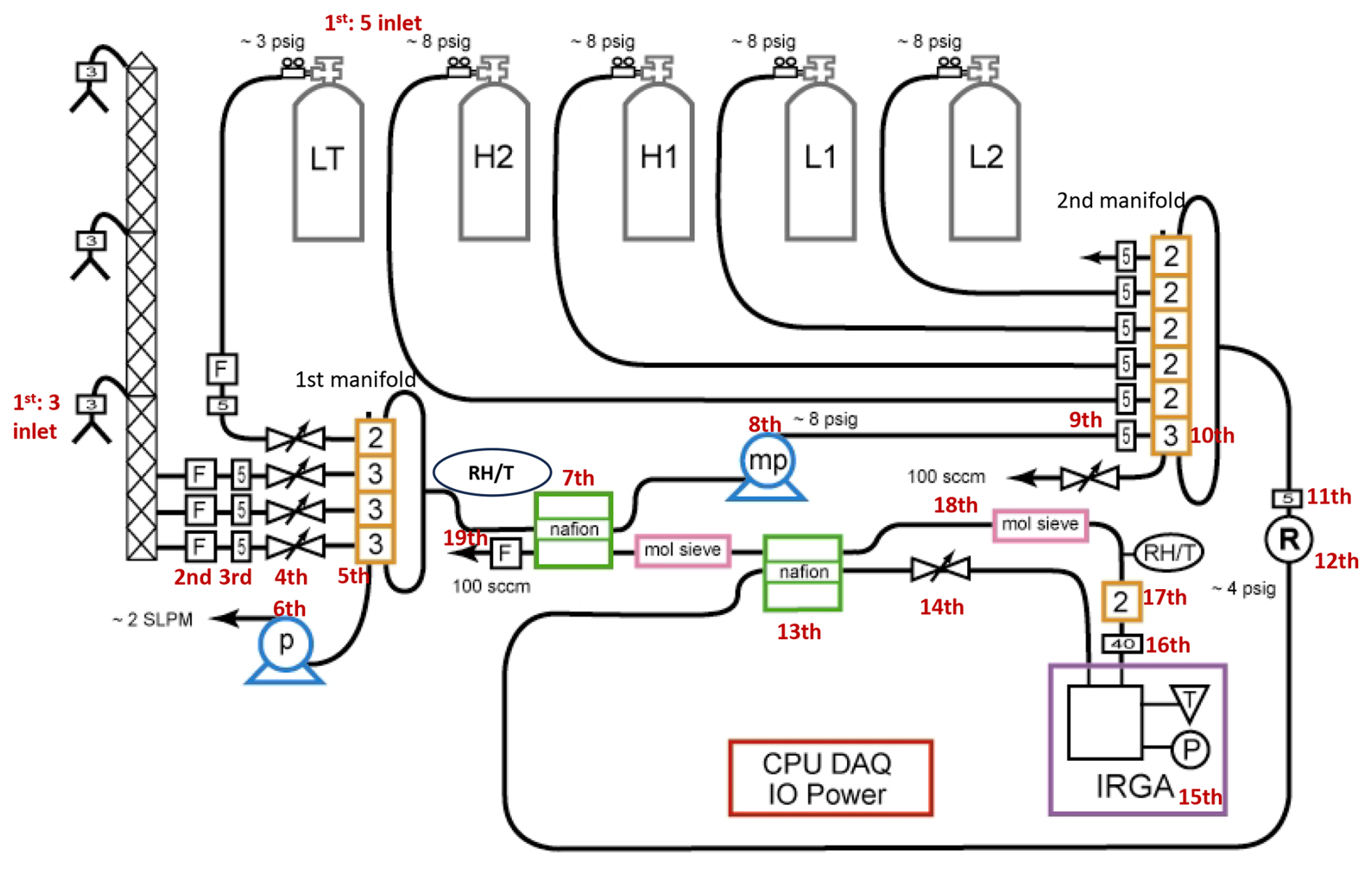
Figure 2 Schematic diagram of the 5-calibration inlet and 5-sample inlet AIRCOA system that was operational in the Loobos first tower. This figure is adapted from Stephens et al. (2006) and only 3 inlets are shown for simplicity. The 5 calibration inlets are taken from the H2, H1, L1, L2 and LT cylinders, where LT stores a long-term surveillance gas for verifying the other four calibration gases. The 5 sample inlets are deployed at different levels in the tower. Each inlet stream (1st) passes through a mass flow meter F (2nd), and a 5 µm metal filter labelled 5 in the following (3rd) and a needle valve (4th) before reaching a manifold of three-way (3) and two-way (2) solenoid valves (5th). A diaphragm pump labelled p (6th) in the blue circle flushes the sample lines to modulate the flow rate (e.g., 2 SLPM (standard liters per minute)) and system pressure. The gas selected by these valves passes through the Nafion driers (7th), and a smaller diaphragm pump in the blue circle (8th) is used to compress the dry gas to increase pressure (e.g., into 8 psig). Then the gas passes through a second 5 µm metal filter (9th) and goes into a second manifold of three-way (3) and two-way (2) solenoid valves (10th). The second manifold selects either a sample gas or a calibration gas for analysis. The select gas then passes through another 5 µm metal filter (11th) and a miniature pressure regulator R in bold (12th). The gas next is dried by a Nafion drier (13th) and reduced in pressure by a needle valve (14th), which is normally used to adjust the sample flow to 100 sccm (standard cubic centimeters per minute). The gas is then analyzed by a LI-820 Infrared Gas Analyzer for measuring CO₂ mole fraction and pressure and temperature (T and P) as well (15th). After leaving the IRGA, the gas goes through a metal filter of 40 µm (16th) and a valve used for leak check purposes, and a humidity and temperature sensor (RH$/T$) to verify drier performance (17th). The gas is further completely dried by molecular sieve (18th), and then goes through a final mass-flow meter (19th) followed by exhausting to the atmosphere at the end.

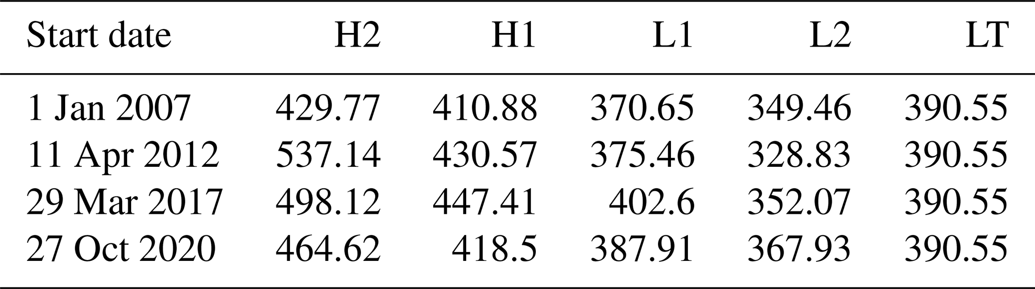
The IRGA datalogger was configured to record raw data in two seconds interval. Regarding the measurement accuracy, the two second filtered values exhibited one standard deviation root mean square error of 0.6 ppm, which averaged to 0.1 ppm over 100 s. The absolute accuracy of the CO₂ mole fraction measurements with the AIRCOA system was 0.2 ppm higher than 2 ppm with the CIRAS system (Elbers et al., 2011). The instrument switched the gas being analysed every 160 s in this case. Every 4 h the instrument measured all four calibration gases to obtain an estimate of the calibration coefficients for the IRGA, and every 8 h the instrument analysed the long-term surveillance gas (LT in Fig. 2). The CO₂ mole fractions in five calibration cylinders provided by University of Groningen were steadily maintained throughout the whole period and the corresponding collected calibration data are listed in Table A1 in Appendix for reference. Additionally, air temperature, wind speed and relative humidity measurements were collected at two more levels below the canopy (7.5 and 5.0 m, Table 1).

2.1.4 Soil properties, soil heat flux, profile soil moisture and soil temperature and soil respiration

Soil heat fluxes were measured by four thermopiles under the litter layer at a depth of 3 cm in the mineral soil at a total depth of 10 cm. Thermopile sensors arranged in a thin ring (similar in design to FHF05 series heat flux sensors, https://www.hukseflux.com/products/heat-flux-sensors/heat-flux-sensors/fhf05-series-heat-flux-sensorss, last access: 15 December 2024) built by Hukseflux were used. After serious lightning damage to the sensors in January 1998, two new sensors (TNO, PU43T and SH1-Hukseflux thermal sensors, Table 1) were placed in November 1998 and remained operational until September 2017. This sensor was located in between the two soil moisture profiles (described below) directly on the mineral soil under the litter layer. Since September 2017 the HFP01SC soil heat flux plate (https://www.campbellsci.com/hfp01sc-l, last access: 15 December 2024) was deployed near the location for measurements until 18 March 2023.

A change of systems throughout the long measuring period occurred as well for soil temperature, electrical conductivity and soil moisture measurements, which were initially measured at five different depths in two profiles 1.5 to 2.0 m apart. The MUXCOM (IMAG-DLO, Multiplexed Control and Monitoring) system containing frequency domain sensors at the 20 MHz frequency range was deployed in two profiles for measurements until 31 December 2004. Every 30 min a measurement was made at all sensors and stored on a palmtop PC. On 11 April 2005 Campbell water content reflectometer sensors CS616 at the 70 MHz frequency range were deployed in one profile and remained operational until 31 May 2023 (Table 1). The Campbell sensors were logged by a Campbell logger that recorded all soil measurements at 30 min intervals. To obtain an accurate estimation of the soil moisture content, calibration curves were made using undisturbed soil samples with a diameter of 20 cm and a height of 20 cm taken at different depths.

Soil respiration measurements were conducted from 2001 to 2010 along one transect with 22 sampling points, extending from the tower to an open area (at the time of measurement, Fig. 1). The transect included both updune and lowdune locations. At each point, the collar was inserted into the soil with a depth of 15 cm and the soil respiration chamber was then placed onto the collar. The grass within the chamber (i.e., SRC-1 soil respiration chamber in this case) was cut if necessary, in order to exclude photosynthesis and plant respiration measurements. Soil CO₂ fluxes were measured using an EGM-4 infrared gas analyser (PP Systems, Table 1) with built-in soil temperature sensors. Soil moisture was simultaneously measured with Theta Probes (Delta-T Devices).

2.1.5 Vegetation properties

Tree inventory

Vegetation properties such as tree diameter at breast height and tree height were measured from 1996 to 2012 (Fig. 1). The main tree species is Pinus sylvestris (Moors, 2012), given the measured tree diameter and height, the above ground biomass (Table 6) was estimated by using the allometric relations (See Eqs. S1 and S2 and Table S1 in the Supplement).

Leaf Area Index (LAI)

The Leaf Area Index (LAI) was measured regularly between 1996 and 2014 with two LAI-2000 (Li-COR) simultaneously. Measurements were typically conducted biweekly during the growing season and monthly otherwise. One instrument was mounted atop the scaffolding tower providing a reference measurement of incoming light. Meanwhile, the other was used along the transect (Fig. 1) below the canopy measuring light attenuation, as such, LAI estimation was made. The setup consisted of 70–100 measurement points with a 3 m spacing below the canopy to provide better spatial representation. The LAI-2000 sensor measurements were calibrated by comparing them with results from destructive sampling (Moors, 2012). The LAI data are listed as ancillary data. Additionally, the Campbell thermistor was deployed since 11 April 2005 to measure bole temperature.

Sap flow

At the Loobos site sap flow was measured (Fig. 1) with a Tissue Heat Balance-system of Čermák (Ecological Measuring System, model P4.1, Brno, Czech Republic) from 1996 to 1998. By measuring temperature changes of the phloem, the amount of energy needed for heating and the specific heat of water, the sap flow was calculated without the necessity of calibrations (Lundblad et al., 2001). Detailed information can be found in Moors (2012).

Between 2012 and 2015 the sap flow was measured with thermal dissipation probes (Dynamax, Table 1) based on the temperature difference between the heated needle and the sapwood ambient temperature. Sapflux was calculated following Granier (1987). The supplied data were averages of two sensors deployed at six trees. The data gaps were mainly due to power shortages and mainly during nights and winter.

Needle foliage properties

A number of needle leaves from trees around the tower were collected to measure needle foliage area, dry weight and leaf mass per area. The foliage area was determined using image analysis software (https://imagej.net/ij/, last access: 11 March 2026), the dry weight was obtained after oven-drying at 60 °C, and the leaf mass per area was calculated as the ratio of dry weight to foliage area. Total carbon (C) and nitrogen (N) concentrations were determined using dry combustion of ground plant material with a CHNS/O elemental analyzer (PerkinElmer 2400 Series II). Total phosphorus (P) concentration was measured by digesting ground leaf material in 37 % hydrochloric acid (HCL) followed by colorimetric measurement at 880 nm after reacting with molybdenum blue.

Photosynthesis measurements involving the light response curve, CO₂ response curve and the daily and seasonal responses of photosynthesis were conducted with an intelligent portable photosynthesis system (ADC Bioscientific Ltd., Table 1). The measurements between 1997 and 1998 were performed on the top of the tower for sun-exposed leaves, and the measurements in 2000 were performed on the top of a tree randomly selected in the north of the tower (Fig. 1). The experiments of obtaining light and CO₂ response curves were conducted for two summer days in 1997 (7, 18 August) and 2000 (19, 20 July), and daily response measurements were on 11 August 1998. The seasonal response of photosynthesis was measured on 29 July 1997, 4, 11, 21 August 1997, 22 November 1997, 12 July 1998. Data of CO₂ assimilation rate, transpiration rate and stomatal conductance at the leaf level were obtained.

2.1.6 Ground water level

The data of the ground water level (GWL) were measured manually in two observing tubes (2.5 cm diameter, Fig. 1). The error in the measurements is less than 1 cm. Due to the dunes there is a distinct local topography with a variation in height of about 2 m in the immediate surroundings of the tower, but at distances more than 100 m away, the dunes may reach 10 m above the valleys. It is unknown how this orography influences the GWL. Data presented as ancillary are from a tube (B15) ±30 m northeast of the flux tower in a local valley ± 2.7 m below the base of the flux tower.

Figure 3 The workflow for processing data from the first tower at Loobos.

2.2 Data processing

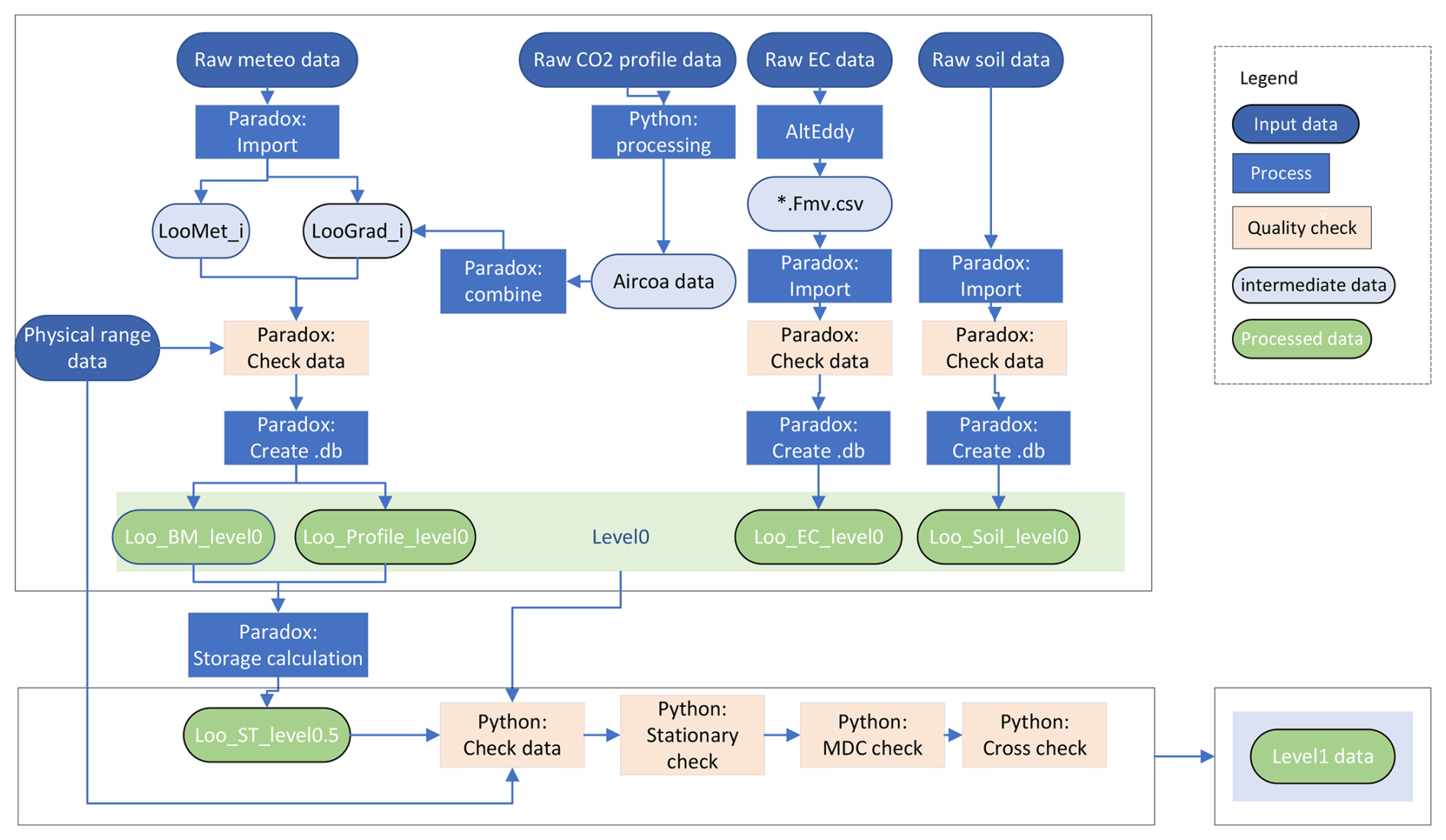
The general processing pipeline for continuous recorded datasets is schematically shown in Fig. 3. The recorded meteorological raw data was imported into a Paradox relational database management system and categorized into two streams: NL-Loo_BM and NL-Loo_Profile, where NL refers to the Netherlands and Loo denotes the site name.

The NL-Loo_BM stream contains fundamental meteorological variables, while the NL-Loo_Profile stream primarily includes profile CO₂ and H₂O pressure data, which were derived from processing PP system and AIRCOA system measurements as described in Sect. 2.2.1. Following this, heat storage and fluxes beneath the canopy were calculated as described in Sect. 2.2.2. The recorded raw EC data were processed using AltEddy software to estimate fluxes (Elbers et al., 2011), as described in Sect. 2.2.3. The resulting flux data, along with the recorded raw soil moisture and temperature data were also imported into the Paradox database. Data quality was verified using predefined physical ranges (Table E1 in Appendix E), and the data was further completed on a yearly scale by replacing missing data with NA values to ensure consistency across all datasets (Fig. 3). By combining meteorology, storage, EC and soil data, the net ecosystem exchange (NEE) rate of CO₂, latent heat flux (LE) and sensible heat flux (H) were computed with NEE being gap-filled, as described in Sect. 2.2.4. In total, four level 0 data streams – NL-Loo_BM, NL-Loo_Profile, NL-Loo_EC and NL-Loo_Soil – were obtained (Fig. 3), together with a level 0.5 data stream of NL-Loo_ST that were derived from the Level 0 dataset. Level 0 implies raw data, as observed and/or based on basic computations. Level 0 and Level 0.5 data which undergo extensive quality control are lifted to Level 1 data.

Additionally, the datasets of soil respiration, vegetation properties (i.e., tree height, stem width and dry aboveground biomass, Leaf Area Index, sap flow, needle foliage properties and the associated nutrient analysis, and photosynthesis response curves) and ground water level are stored as ancillary data.

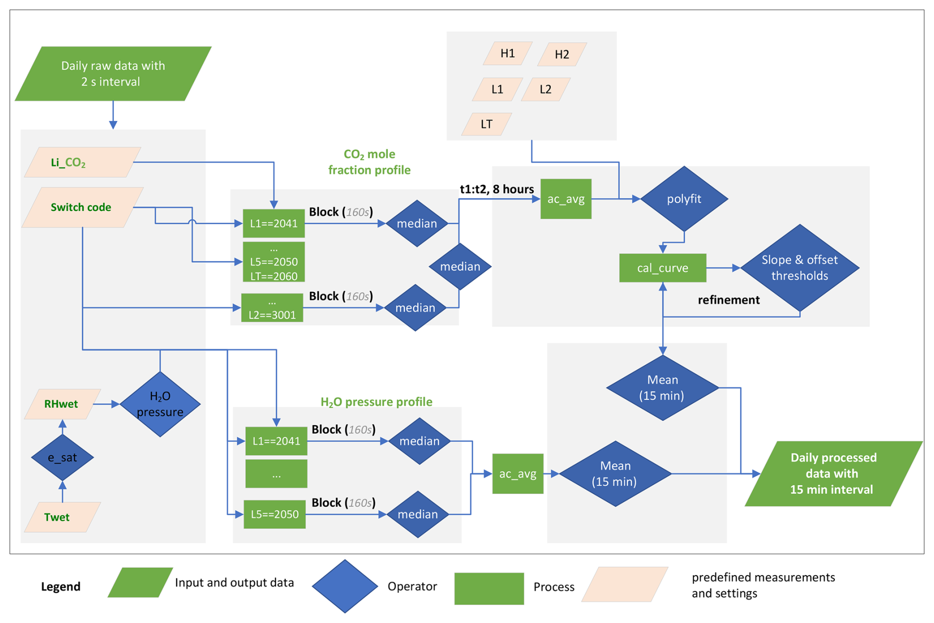
Figure 4 Flowchart for processing profile CO₂ mole fraction (ppm) and H₂O pressure (mbar) measured by AIRCOA.

2.2.1 Calculation of profile CO₂ mole fraction and H₂O pressure

Using the recorded raw data at two-second intervals and the collected calibration data, CO₂ mole fractions at the five altitude levels were calculated, as illustrated in Fig. 4. The main procedures included (1) Screening the line data to match the appropriate level, (2) Calculating median values for each data level over a time block of 160 s, corresponding to the gas switch frequency in this case, (3) incorporating calibration data into each block, (4) Computing calibration curves for each eight hour cycle based on LT operation cycle, (5) Applying calibration coefficients to the level data at 15 min intervals. The calibration effects can be viewed in Figs. C1 and C2 in Appendix C.

The water vapor pressure at the five levels was derived from the measured relative humidity and temperature of the sampled gas before it entered the drying system (see Fig. 4), using standard equations (Eqs. B1–B2 in Appendix B). Since H₂O sensors are stable and less affected by interferences from other gases and environmental factors, no additional calibration was required, unlike the CO₂ mole fraction measurements. The same aggregation method was applied to obtain the profile of the H₂O mole fraction at 15 min intervals. The flowchart illustrating the calculation process for the profile CO₂ and H₂O mole fraction is presented in Fig. 4.

2.2.2 Calculation of heat storage and fluxes beneath the canopy

Sensible fluxes of sensible heat beneath the canopy were derived from the measured air temperature at the three levels, following the equations outlined in Appendix D (Eqs. D1–D2). In a similar manner, CO₂ and H₂O storage fluxes were derived using the measured CO₂ mole fraction and water vapor pressure at five levels. The storage data was saved for use in the NL-Loo_ST_level0.5 stream.

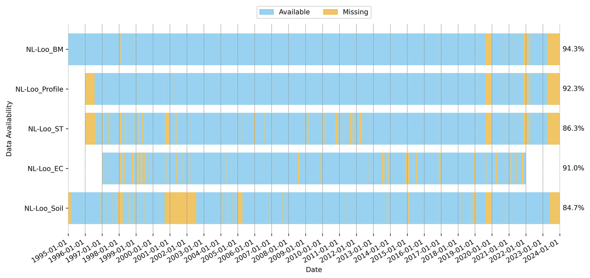
Figure 5 The availability of the five continuous data streams. NL-Loo denotes the origin of the site. The NL-Loo_BM stream includes biometeorological data, the NL-Loo_Profile stream contains vertical profile data, the NL-Loo_ST stream includes storage data, the NL-Loo_EC stream includes EC measurement data, and the NL-Loo_Soil stream includes soil moisture and temperature data.

2.2.3 Estimate of turbulent fluxes

The turbulent fluxes are estimated as covariances between vertical wind speed and the scalar quantities of interest (heat, water vapor, CO₂). To derive these flux estimates from the raw EC measurements, the AltEddy software (Version 3.90, from Wageningen Environmental Research (WEnR), The Netherlands) was used. This software executes a series of essential processing steps, including detrending, time-lag correction, double coordinate rotation correction to align wind velocity components with the mean wind direction, angle of attack correction, density fluctuation compensation (Webb et al., 1980), normalized spectra and cospectra calculations. Detailed information about AltEddy software can be found at https://climate-data.nl/climatexchange/projects/alteddy (last access: 11 March 2026), see also Mauder et al. (2008), which demonstrated the capability of the AltEddy software in calculating CO₂ fluxes compared to those calculated by other software packages. The output data saved in the NL-Loo_EC_level0 stream contains the turbulent and CO₂ fluxes and the corresponding quality flag from Foken et al. (2004), as well as the means of wind and scalars and the turbulent and flux parameters including friction velocity (u^*), stability parameter $z/L,$ wind direction and the 80 % distance integration of the flux derived from Schuepp et al. (1990).

2.3 Data quality control

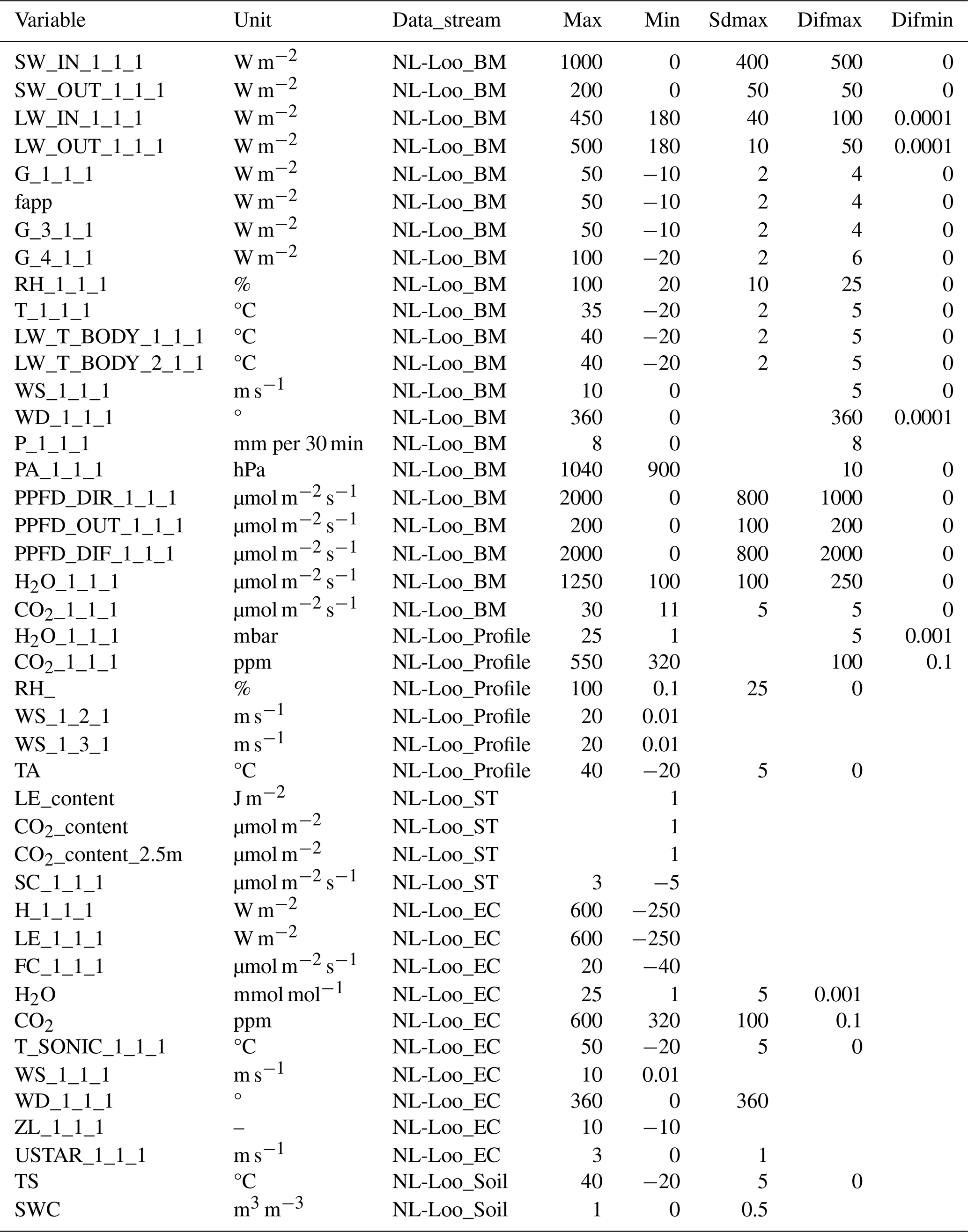
Physical data ranges, including maximum and minimum values, maximum and minimum values of differences between consecutive time steps, and the maximum standard deviation of the interest of field, were applied to filter out abnormal values and missing data from level 0 NL-Loo_BM, NL-Loo_Profile and NL-Loo_Soil streams, as illustrated in Fig. 3 (light orange box). Table E1 in Appendix E shows the maximum and minimum physical ranges, maximum differences, and maximum standard deviations applied for variables.

Regarding the turbulent fluxes and CO₂ flux from the NL-Loo_EC stream, an initial quality flag was produced by running the AltEddy software. The data quality was further refined (Fig. 3). Specifically, flux subset data were created and used for the determination of the response of daytime flux to incoming solar radiation and of nighttime flux to air temperature. Subsequently, flux data were discarded when they fell outside tolerable ranges (a bin-average ±2 standard deviation), and the corresponding quality flag data were reassigned accordingly. Detailed descriptions can be found in Elbers et al. (2011).

The level 0 and level 0.5 data was further reviewed and refined into consistent level 1 data through four procedures (1) reapplying physical range criteria (Table E1), (2) filtering out stationary data within a three-hour window (with the exception of the NL-Loo_Soil stream and shortwave radiation in the NL-Loo_BM stream), (3) calculating the long-term mean diurnal cycle (MDC) and its standard deviations for CO₂ flux and accordingly filtering out daytime data not in the tolerable range, and (4) comparing similar fields from different streams for cross-checks.

We thus provide a level 1 data product, which consists of quality controlled measured variables and derived variables (e.g. eddy fluxes and storage fluxes). Here we do not provide gap filled data, since the gap-filling will be done centrally by ICOS/FLUXNET in a homogenised way. We anticipate that the gap-filled data will become available via ICOS and FLUXNET as part of the net FLUXNET Data System by December 2025.

2.4 Period of record

Please refer to the description Excel sheet to review the variables included in each data stream. The Level 1 data were stored in one CSV file per stream, where the variable name is consistent with ICOS standards. The ancillary data were stored in Excel per stream. Level 1 data availability is presented in both Fig. 5 and Table 1.

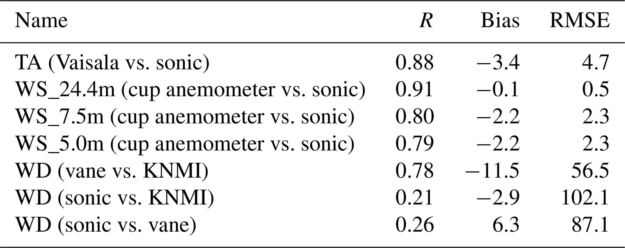
Table 2 Statistics comparing meteorological data measured by different sensors from 1997 to 2022. TA is expressed in °C, WS is in unit of m s⁻¹ and WD in degrees.

3 Data evaluation

3.1 Data cross-checks

To validate the meteorological data measured by various sensors, statistical metrics including Pearson's correlation coefficient (R), mean bias (Bias) and root mean square error (RMSE) were calculated for air temperature (TA) measured by Vaisala against sonic temperature, profile wind speed (WS) measured by cup anemometer against WS from sonic, and wind direction (WD) measured by the wind vane and sonic against WD from KNMI meteorological station at Deelen (https://www.knmi.nl/nederland-nu/klimatologie/daggegevens, last access: 11 March 2026), the closest KNMI station to the Loobos first tower. Table 2 shows high R values for temperature and WS measured by different sensors. Compared to WD measured by sonic, the WD measured by the wind vane exhibits higher R and lower RMSE when compared with the KNMI daily dataset. The use of WS and WD from the wind vane is thus recommended for further analysis. Table 3 shows decent correlation coefficients (> 0.5) between CO₂ mole fraction and H₂O pressure measurements from the AIRCOA system and those from the EC system. These cross-check results demonstrate the consistency of datasets measured by different sensors.

Regarding vegetation data, the tree height (Table 4) matches well with the tree height measured in the target area in the current years (Table 3 in van der Molen et al., 2026). Two datasets suggest a growth rate of 16 cm yr⁻¹. As the Pinus sylvestris species dominate in the study area (Moors, 2012) during the period from 1996 to 2025, by assuming the average tree density of 499.1 trees ha⁻¹, the above ground biomass was estimated by using the allometric relations (see Supplement)) and measured tree height (Table 4) and diameter (Table 5). A larger biomass during this period (Table 6) is observed than that in the 2023 inventory based on over 1000 trees (van der Molen et al., 2026). Nevertheless, the estimated biomass is in the same order of magnitude.

Table 3 Statistics comparing profile CO₂ mole fraction and H₂O pressure data measured by different sensors at different altitude levels (from 1 to 5 representing 24.4, 7.5, 5.0, 2.5 and 0.4 m) in the canopy. CO₂ is expressed in unit of ppm and H₂O in mbar.

Table 4 Tree height measurements between 1996 and 2025.

Table 5 Tree diameter measurements between 1996 and 2025.

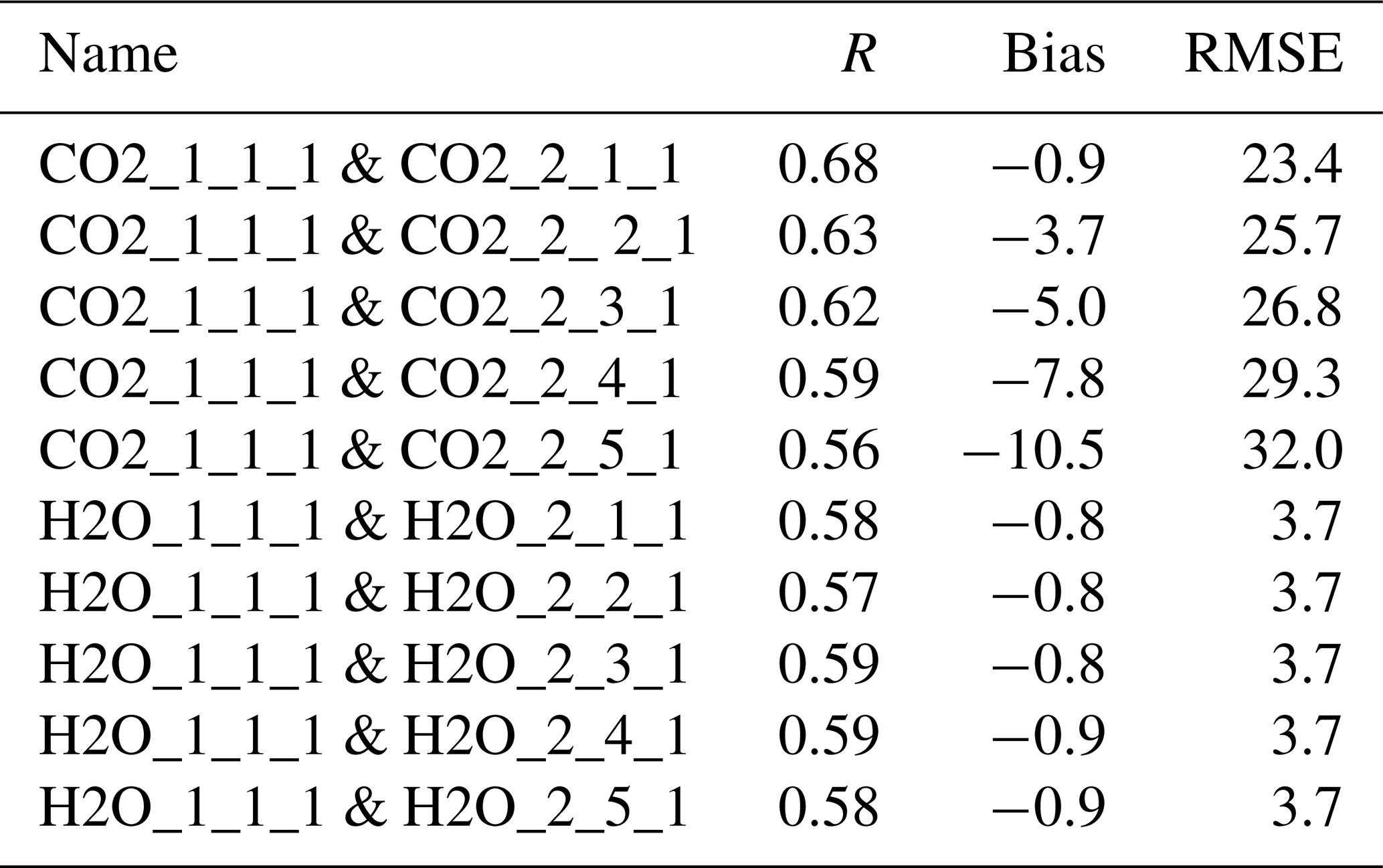
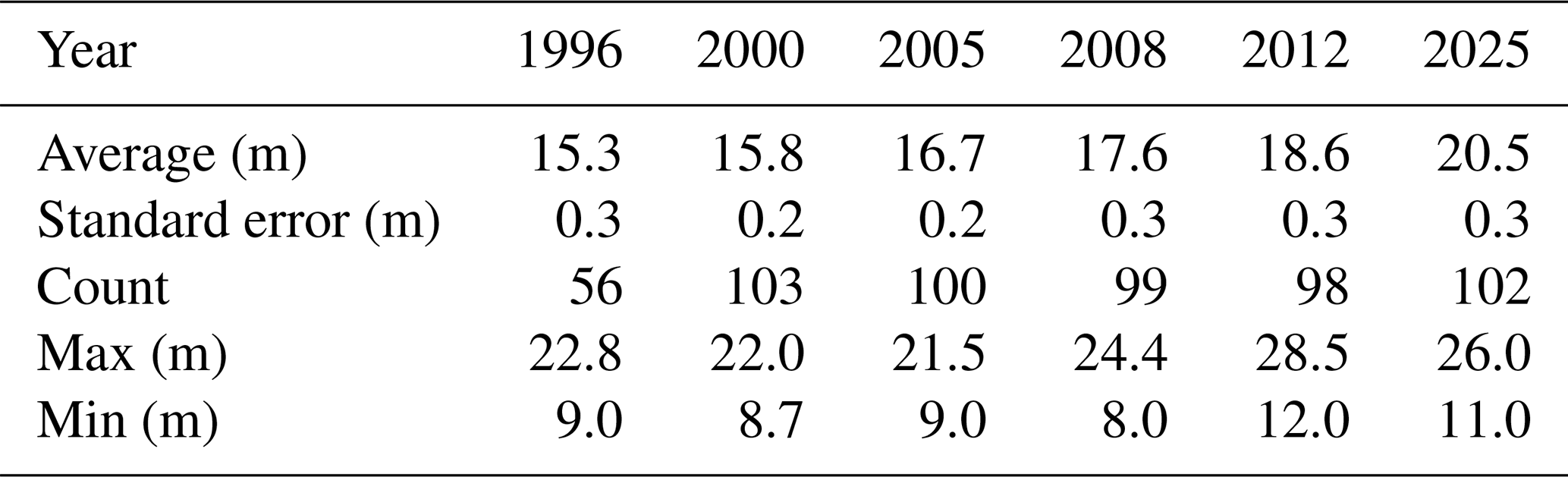
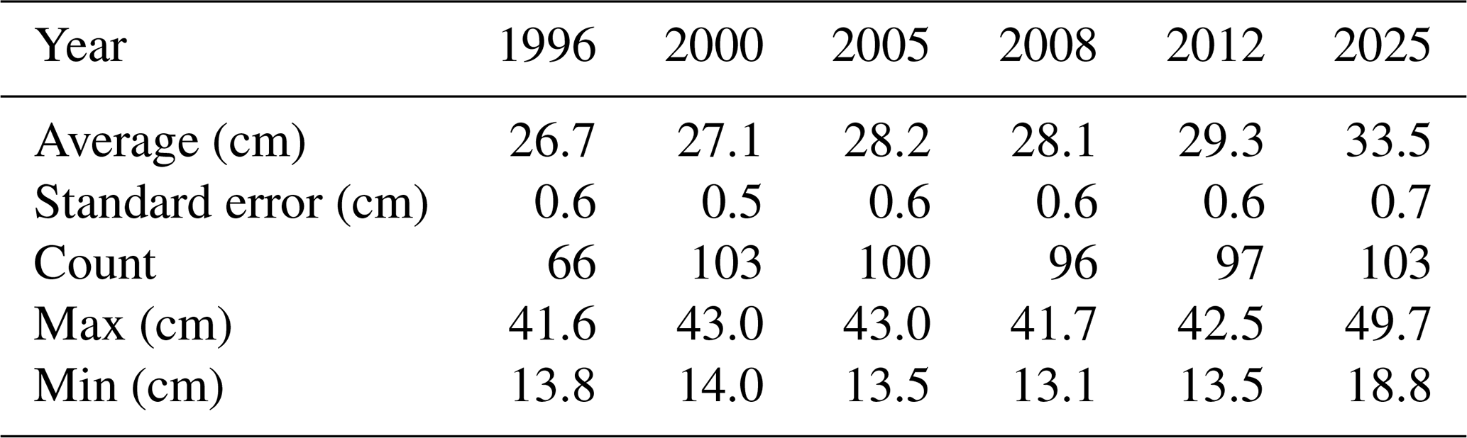
Table 6 Above ground biomass (ton dry matter ha⁻¹) estimated between 1996 and 2025. The 1996 tree density is low relative to 2000. In brackets the 2000 tree density and the resulting total above ground biomass estimate.

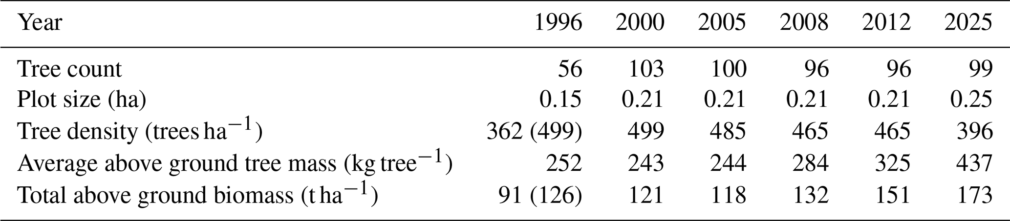
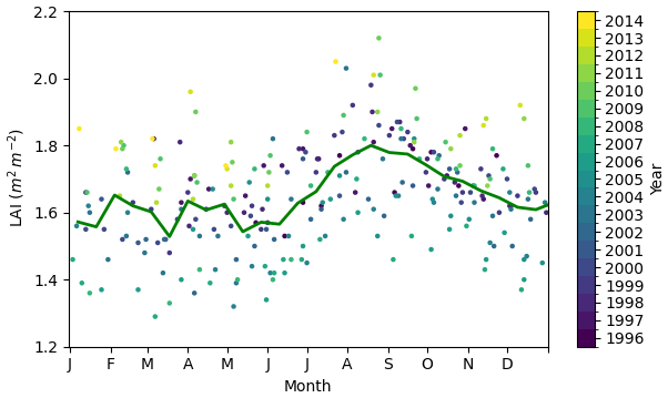
Figure 6 Seasonal cycle of Leaf Area Index. The colored points indicate the individual measurements and their year of measurements. The solid line shows the 14 d mean. Each data point is the average of 60 samples collected 10 m apart in two 300 m transects crossing at the first tower. The tick marks on the x-axis indicate the first day of the month.

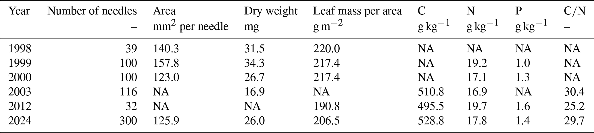
Table 7 Area, dry weight and concentrations of carbon, nitrogen and phosphorus in foliar samples from 1998 to 2024. NA – not available

Here the tree density in 1996 is based on an inventory of 150 trees, while only for 56 trees the height and diameter were measured. Information about the plot size and consequent tree density in 2000 has been lost. By plotting the tree coordinates on a map, it has been derived that the plot size must have been between 45×45 and 50×50 m. A written report claims a tree density of 499.1 trees ha⁻¹ in 2000 which is consistent with 103 trees in 0.21 ha (45.4×45.4 m). This is the plot size we assumed. In subsequent years, the tree density was decreased with the number of fallen trees in the inventory. In 2025 68 of the 103 original tree tags have been found. Others have disappeared or grown into the bark. In addition, 31 untagged trees were found in a 50×50 m square around those 68 trees. This implies that the tree density decreased from 465 in 2012 to 396 trees ha⁻¹ in 2025, a decrease of 17 trees in the quarter hectare plot in 13 years, which seems realistic considering the number of dead stems observed in the field. However, some stems have completely been decomposed in the meantime.

The resulting LAI is 1.65 on average, but variable over the season (Fig. 6), with an increase after budburst in late spring and early summer, a clear maximum in August and a decline in fall, associated with partial leaf shedding. A distinct inter-annual variation was observed (Fig. 7), although it is unknown what the underlying cause is, we note that storms in 2007 caused trees and tree tops to break and 2003, 2013 to be dry years, 2007 and 2008 to be wet years. Additionally, Table 7 presents comparable needle foliage attributes measured between 1998 and 2012 with those from 2024 (van der Molen et al., 2026).

3.2 Mean diurnal storage CO₂ flux

The mean diurnal cycles of the CO₂ mole fraction gradients (d${\mathrm{CO}}_{\mathrm{2}}/$dz) shown in Fig. S2 demonstrate a coherent and physically consistent vertical structure, with the strongest gradient occurring near the surface during nighttime and early morning hours, and a progressively weaker gradient towards higher levels. In extreme situations, i.e. in the summer months June, July and August, when the respiration fluxes are large and with u^* < 0.3 m s⁻¹, the gradients are typically 1 ppm m⁻¹ between 25 and 7.5 m, 2 ppm m⁻¹ between 7.5 and 5.0 m and 5 ppm m⁻¹ below there. These findings indicate that the selected sampling heights adequately resolve the dominant features of the vertical CO₂ concentration profile relevant for calculating the column-integrated storage term.

Figure 7 Interannual variation in Leaf Area Index.

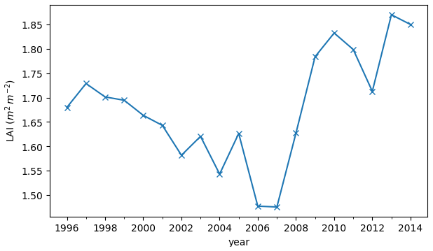
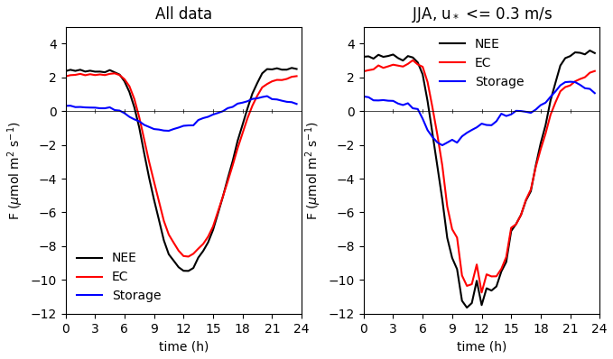
Figure 8 Magnitude of NEE (total CO₂ flux), and the individual EC and storage components at a height of 27 m, visualised as the mean diurnal cycle of all available data (left) and under conditions of low turbulence ($u^{\ast }<\mathrm{0.3}$ m s⁻¹) and large respiration fluxes in summer (JJA denotes June, July and August).

To understand how large the storage CO₂ flux is as a fraction of total CO₂ fluxes, the mean diurnal variations of NEE (total flux), EC and storage measurement were calculated separately (Eq. F1 in Appendix F). Figure 8 shows the magnitude of NEE (total flux) and the EC and storage components. The CO₂ storage flux is typically in the order of 1 µmol m⁻² s⁻¹, but in extreme situations it can be between −5 and +3 µmol m⁻² s⁻¹. At moments around sunrise and sunset, the EC fluxes are close to zero, while the (negative) storage flux is largest around sunrise, indicating a release of carbon dioxide stored below the canopy at night. At the same time, plant photosynthetic uptake of CO₂ begins, partially offsetting this upward flux. Surprisingly, the release continues well until noon. In cumulative fluxes on a daily or longer timescale, the storage flux is negligible, but on hourly timescales the storage flux needs to be taken into account to represent the true ecosystem CO₂ fluxes. Concludingly, the CO₂ storage flux is a significant but small fraction of the total NEE.

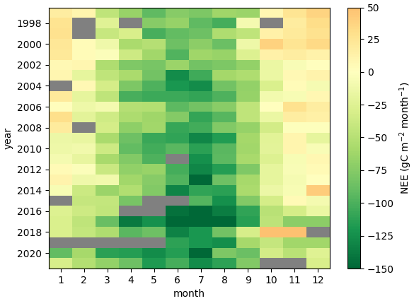
Figure 9 Seasonal and interannual variation in net carbon dioxide exchange, based on the eddy covariance measurements. The values represent the monthly mean diurnal cycle integrated to a monthly total. Gray colors indicate a data availability less than 30 %.

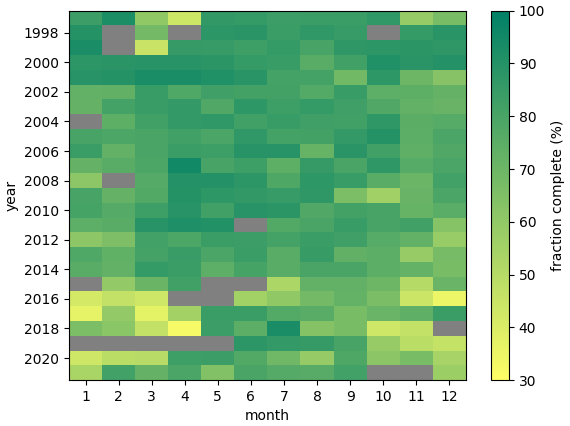
Figure 10 Completeness of the eddy covariance carbon dioxide data. Gray colors indicate a data availability less than 30 %.

3.3 Seasonal and interannual variations in NEE

In an effort to verify the consistency of the EC dataset of carbon dioxide exchange over the years (Zhao et al., 2025), we show the mean monthly NEE per year (Fig. 9), Subsequently, we calculated the monthly mean diurnal cycle, which we integrated to a monthly CO₂ exchange. Because we integrate the mean diurnal cycle, the storage component may be ignored and hence this estimate represents the monthly NEE. Here we implicitly assume an absence of lateral outflow of nocturnal storage fluxes. The figure shows a clear and consistent seasonal cycle, with carbon uptake from March to September and release from October to February. The intensity of the CO₂ source appears to decrease over time, whereas the intensity of the summer uptake is increasing. The mean annual uptake between 1997–2006 is around 350 gC m⁻² yr⁻¹ and between 2007 and 2016 around 550 gC m⁻² yr⁻¹. In 2018 and 2019 the mean uptake grew to an average of 820 gC m⁻² yr⁻¹, partially because of the reduction in wintertime net fluxes.

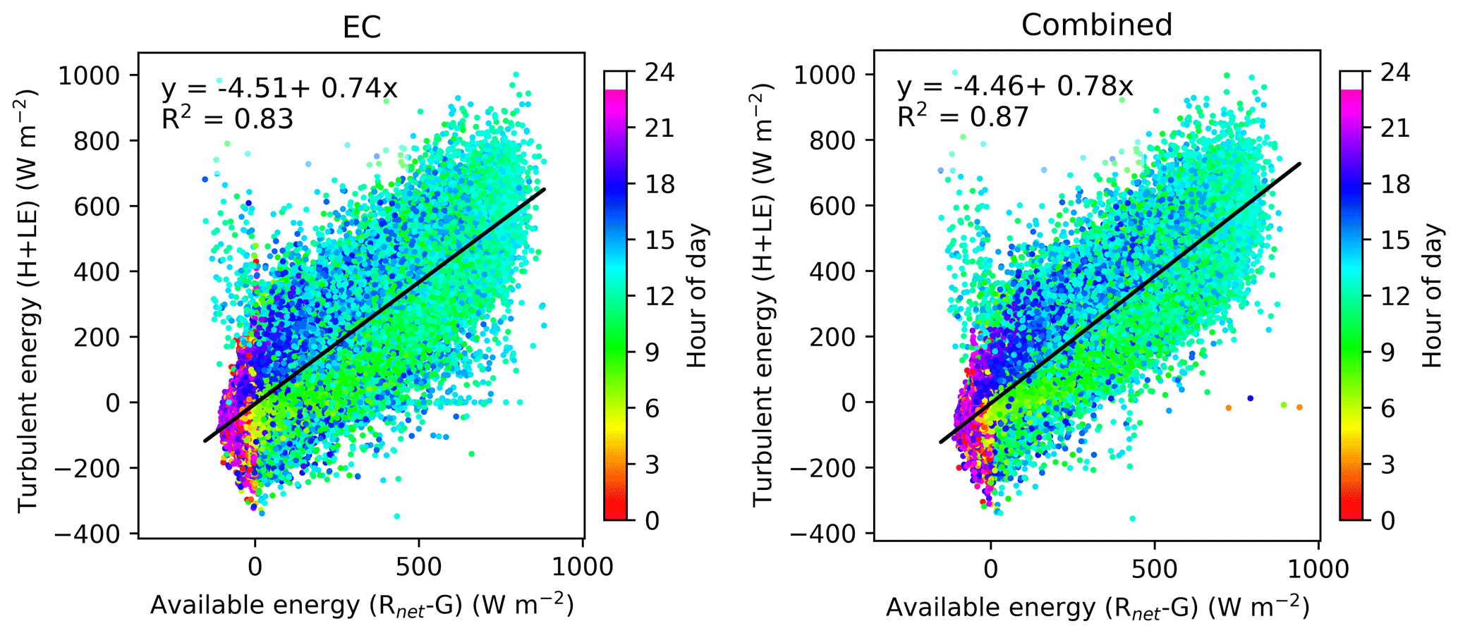
Figure 11 Energy balance closure of the Loobos first tower datasets at a height of 27 m. The left graph shows turbulent fluxes based solely on EC fluxes, and the right graph indicates turbulent fluxes combined with storage fluxes.

We stress that this dataset is based on eddy covariance measurements and is not gap-filled. Figure 10 shows the completeness of the dataset. Without u^∗ filtering all months have a completeness larger than 85 % of the half hours. The u^∗ filtering reduces the completeness to an average of 82 %, not considering the periods with fully lacking data. Upgrading Level 1 data into a Level 2 gap-filled dataset and analysing the trend of NEE, total LE and H are beyond the scope of this study.

3.4 Energy balance residual

The energy balance closure (R_net-G vs. LE+H) was calculated. With the inclusion of storage fluxes of water and heat, Fig. 11 demonstrates an improved energy balance closure, supported by an enhanced regression relationship reflected in the slope and coefficient of determination (R²) between available energy (i.e., R_net-G) and turbulent fluxes (i.e., LE+H), which aligns with findings from previous studies (Leuning et al., 2012). The point colors indicate the hour of the day, suggesting that energy balance closure is lower in the mornings than in the afternoon, which could be related to unaccounted for energy storage in biomass. Detailed analysis of surface energy balance is beyond the scope of this study.

4 Data availability

The Loobos first tower dataset in Level 1 and ancillary data can be accessed at https://doi.org/10.5281/zenodo.15721310 (Zhao et al., 2025) under a CC-BY4 open use license. The Level 1 data will also be available at the European Fluxes Database Cluster. The Level 2 gap filling and partitioning data based on the ONEFlux processing pipeline (Pastorello et al., 2020) for the FLUXNET release will be accessible at the ICOS carbon portal (https://www.icos-cp.eu/observations/carbon-portal, COS Carbon Portal 2026) in Spring 2026.

5 Code availability

The Python codes for processing Level 0 into Level 1 dataset, and for plotting figures shown in the text can be found at https://git.wur.nl/zhao133/nl-loo_first_tower_project.git (Zhao et al., 2026).

6 Discussion and conclusion

Being one of the longest datasets of its kind (https://fluxnet.org/data/la-thuile-dataset/lathuile-data-summary/, last access: 15 December 2024), this long and complete dataset can be used for further data analysis, development and/or verification of models and validating satellite data retrievals. It is noted that in 2021 a second tower was built and equipped next to the first. This second tower was labelled as an Integrated Carbon Observation System (ICOS) class 2 Ecosystem site in 2023 (https://meta.icos-cp.eu/resources/stations/ES_NL-Loo, last access: 15 December 2024, van der Molen et al., 2026). The data from the second tower may be regarded as a continuation of the dataset reported in this work and can be accessed via the ICOS carbon portal (https://www.icos-cp.eu/, last access: 15 December 2024).

The Loobos tower has been running almost without major interruption for more than 25 years now, serving as a robust platform for various scientific studies and educational activities. Over the years, diverse experiments with different objectives have been conducted at and around the tower, ranging from nitrogen deposition research (https://ruisdael-observatory.nl/wp-content/uploads/2018/12/Ewout-Melman-PDF.pdf, last access: 15 December 2024), remote sensing studies (https://ruisdael-observatory.nl/wp-content/uploads/2023/03/New-Loobos-ecosystem-site-compressed.pdf, last access: 15 December 2024) to educational activities for field training courses at Wageningen University. In summary, in addition to its role as a unique and well-equipped platform, the Loobos site offers a rich data set for continued research and analyses.

As a component of the Ruisdael Observatory (https://ruisdael-observatory.nl/loobos/, https://maq-observations.nl/, last access: 15 December 2024), the Loobos Pine forest site represents one of the major land surface types in the Netherlands. It is typical for the extensive Veluwe region, which is aerodynamically rough, forested, located on well-drained sandy soils and vulnerable to summer drought (Granier et al., 2007). The site is downwind from an area with intensive livestock farming and is exposed to high ammonia deposition. In combination with high NO_x emissions from the cities and highways further upwind, high ozone and particulate matter (PM) mole fractions may develop. Both the high input of reactive nitrogen, and the high ozone and PM concentrations may affect ecosystem growth (de Vries and Du, 2024; Visser et al., 2021; Visser et al., 2022; Grantz et al., 2003). To better understand these dynamics, we intermittently measure ammonia dry deposition fluxes in cooperation with the National Institute for the Environment for Public Health and the Environment (RIVM) and seek further funding to measure fluxes of reactive compounds.

Within the Ruisdael Observatory, the Loobos site, along with the Veekampen site (representing rural grassland (https://maq-observations.nl/, last access: 15 December 2024)) and the Cabauw site (representing rural, grass and peat land (Bosveld et al., 2020)) collectively form a triangle network of comprehensive observation sites. This network provides valuable opportunities to understand changes in the land-atmosphere interaction and validate high resolution climate and land surface models.

Appendix A

A1 Photos taken at Loobos site

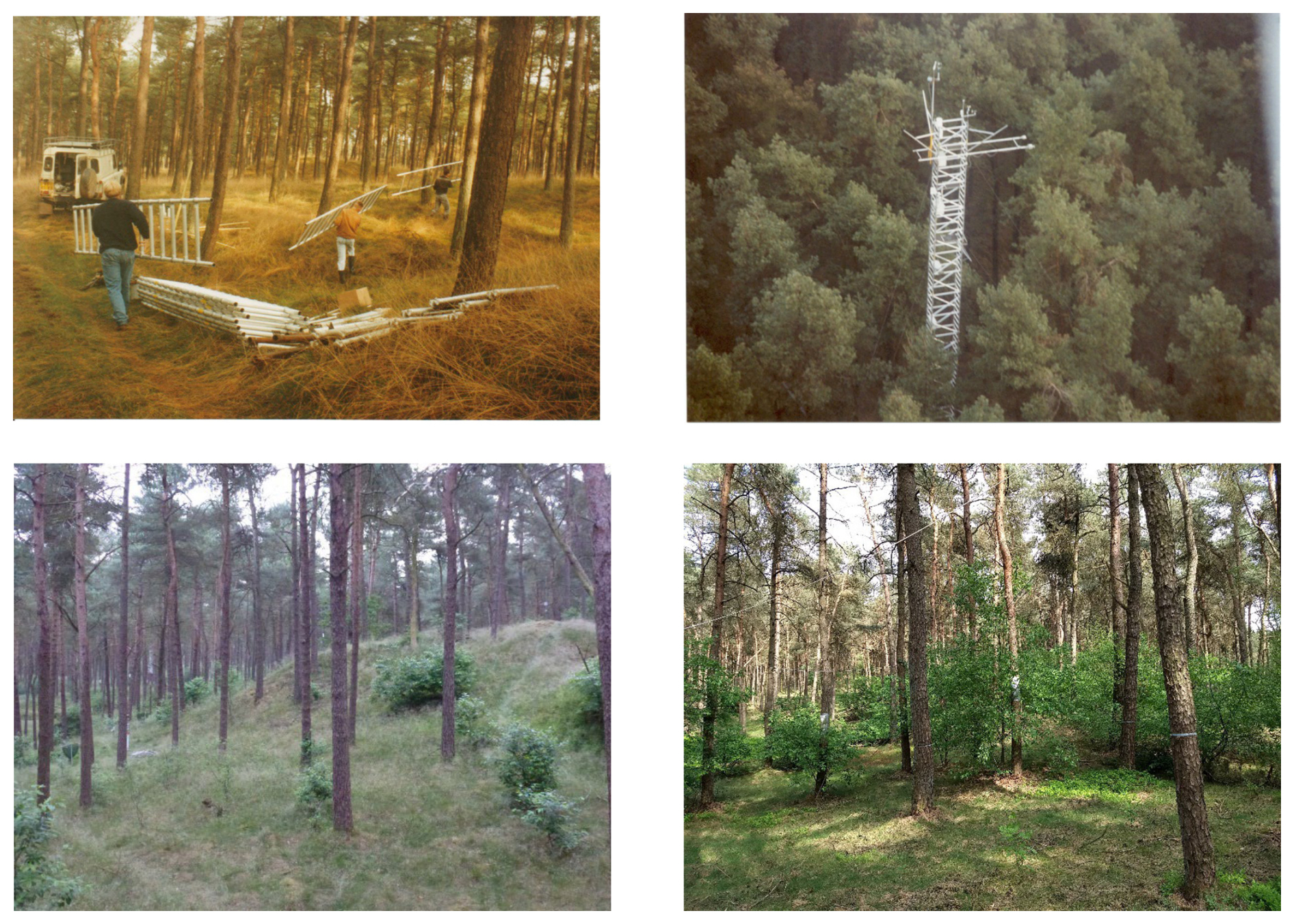
Figure A1 Photos taken at the Loobos site. On the upper panel, the photo on the left was taken in 1995 and the photo on the right sin 2017. On the bottom panel, the photo on the left was taken in 2012 and the photo on the right in 2018.

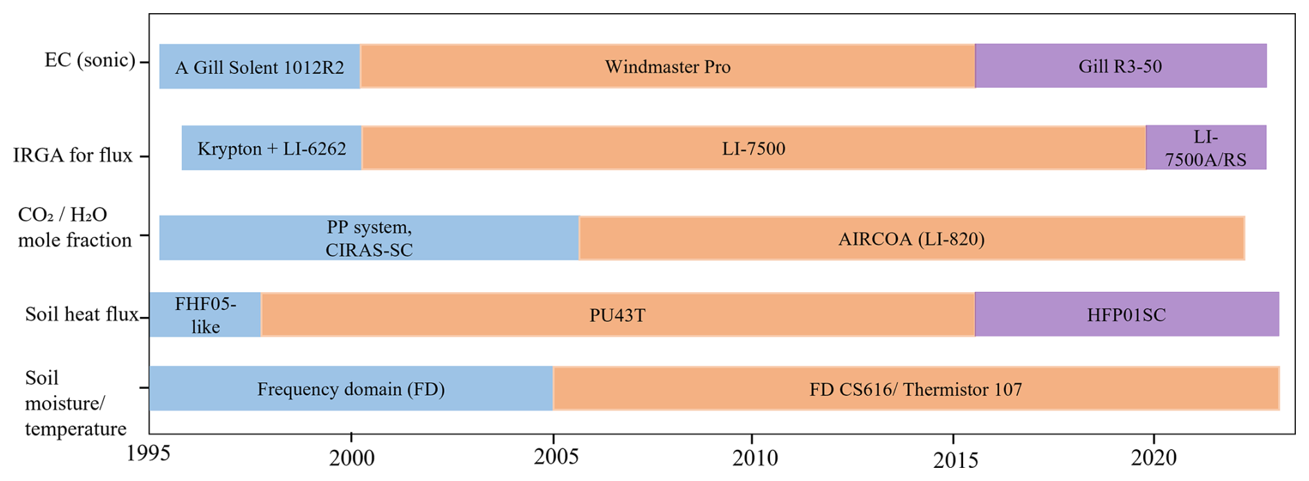
Figure A2 An overview of the changeover information for the main instruments deployed at the Loobos first tower site.

A2 Profile CO₂ mole fraction measurements

The CO₂ profile measurements were calibrated twice a day (Sect. 2.2.1). The table below shows the CO₂ mole fractions in the cylinders.

Table A1 CO₂ mole fraction of calibration cylinders provided by University of Groningen in the AIRCOA system deployed at the first tower in Loobos.

Appendix B: Water vapor pressure calculations

The Maghus-Tetens empirical formula is used to calculate the pressure of saturated water vapor in air (e_sat) at a given temperature (T).

$$\begin{array}{}\text{(B1)}& e_{\mathrm{sat}}=e_o\times {\mathrm{10}}^{\frac{a\cdot T}{b+T}}\end{array}$$

e_o is valued of 6.107 mbar for liquid water. a and b are constants specific to either water or ice. a is valued of 7.5 °C and b of 237.3 °C for water, and a of 9.5 °C and b of 265.5 °C for ice.

$$\begin{array}{}\text{(B2)}& e_{\mathrm{actual}}={\displaystyle \frac{\mathrm{RH}}{\mathrm{100}}}\cdot e_{\mathrm{sat}}\end{array}$$

Appendix C: AIRCOA CO₂ mole fraction calibration results

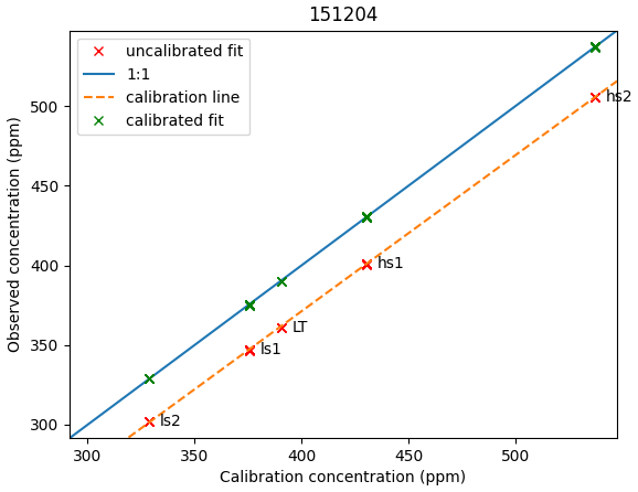
Figure C1 The calibrated CO₂ mole fraction against the observations on 12 April 2015 shown as an example. The ls and hs represent L and H calibration described in the text. The results indicate a good calibration.

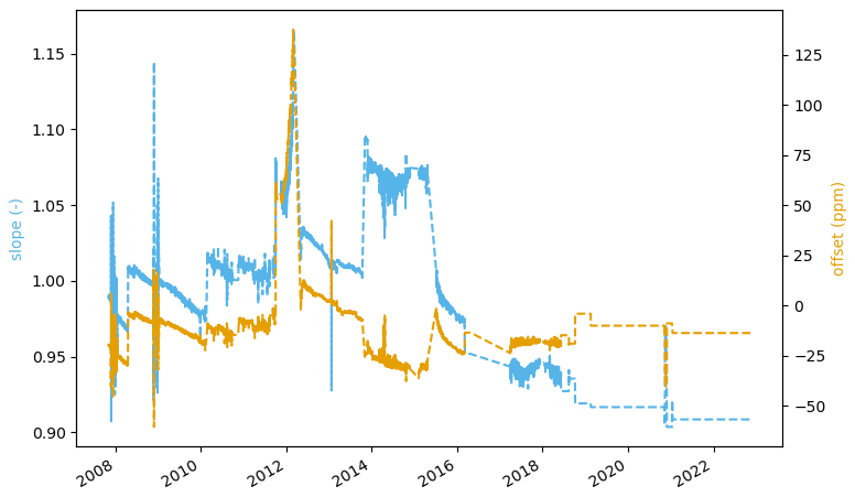
Figure C2 The calibration slope and offset in time series. It shows the value of the slope greater than 0.90 and most values of the offset within 30 ppm.

Appendix D: Calculations of CO₂ and H₂O storages under the canopy

The integrated heat, CO₂ and H₂O mole fraction under the canopy above the ground are calculated by equations below,

$$\begin{array}{}\text{(D1)}& \begin{array}{rl}& \mathrm{H}\mathrm{\_}\mathrm{content}=\sum _{i=\mathrm{1}}^Z\mathrm{\Delta }{z}_i{T}_i{\mathit{\rho }}_i{C}_p(i=\mathrm{1},\mathrm{2},\mathrm{3},\mathrm{4},\mathrm{5},\mathrm{6})\\ & \mathrm{LE}\mathrm{\_}\mathrm{content}=\sum _{i=\mathrm{1}}^Z\mathrm{\Delta }{z}_i{\left[{\mathrm{H}}_{\mathrm{2}}\mathrm{O}\right]}_i{\mathit{\rho }}_{\mathrm{air}}{C}_p{\mathit{\gamma }}_{(T_i,p)}(i=\mathrm{1},\mathrm{2},\mathrm{3},\mathrm{4},\mathrm{5},\mathrm{6})\\ & {\mathrm{CO}}_{\mathrm{2}}\mathrm{\_}\mathrm{content}=\sum _{i=\mathrm{1}}^Z\mathrm{\Delta }{z}_i{\displaystyle \frac{{\left[{\mathrm{CO}}_{\mathrm{2}}\right]}_i}{M}}{\mathit{\rho }}_{\mathrm{air}}(i=\mathrm{1},\mathrm{2},\mathrm{3},\mathrm{4},\mathrm{5},\mathrm{6})\\ & {\mathrm{CO}}_{\mathrm{2}}\mathrm{\_}\mathrm{content}\mathrm{\_}\mathrm{2.5}\mathrm{m}=\sum _{i=\mathrm{5}}^Z\mathrm{\Delta }{z}_{\mathrm{6}}{\displaystyle \frac{{\left[{\mathrm{CO}}_{\mathrm{2}}\right]}_i}{M}}{\mathit{\rho }}_{\mathrm{air}}(i=\mathrm{5},\mathrm{6})\end{array}\end{array}$$

where ${\left[{\mathrm{H}}_{\mathrm{2}}\mathrm{O}\right]}_i$ and ${\left[{\mathrm{CO}}_{\mathrm{2}}\right]}_i$ mole fraction measurements were conducted at five layers of 25.97 (i=1), 7.5, 5.0, 2.5, 0.4 (i=5) m, i=1 denotes the ground layer, and T_i were measured at the three levels (23.5, 7.5 and 5.0 m). The integration starts from the ground level of 0 m. ρ_air denotes air density, which is determined by air temperature, water vapor pressure and air pressure. C_p denotes the specific heat of air (at a constant pressure of 1005.0 mbar) J (kg⁻¹ K⁻¹). ${\mathit{\gamma }}_{(T_i,p)}$ denotes a rate of change related to the latent heat of vaporization, which is determined by air temperature T_i and air pressure p, M denotes the molecular weight of dry air at 0.028966 kg mol⁻¹. H_content and LE_content have a unit of J m⁻², and CO₂_content and CO₂_content_2.5m have a unit of µmol m⁻².

The integrated heat, CO₂ and H₂O fluxes under the canopy above the ground are calculated by equations below,

$$\begin{array}{}\text{(D2)}& \begin{array}{rl}& \mathrm{SH}\mathrm{\_}\mathrm{1}\mathrm{\_}\mathrm{1}\mathrm{\_}\mathrm{1}=\mathrm{H}\mathrm{\_}\mathrm{strg}=\\ & {\displaystyle \frac{\mathrm{H}\mathrm{\_}{\mathrm{content}}_{t+\mathrm{1}}-\mathrm{H}\mathrm{\_}{\mathrm{content}}_t}{\mathrm{1800}}}\\ & \mathrm{SLE}\mathrm{\_}\mathrm{1}\mathrm{\_}\mathrm{1}\mathrm{\_}\mathrm{1}=\mathrm{LH}\mathrm{\_}\mathrm{strg}=\\ & {\displaystyle \frac{\mathrm{LH}\mathrm{\_}{\mathrm{content}}_{t+\mathrm{1}}-\mathrm{LH}\mathrm{\_}{\mathrm{content}}_t}{\mathrm{1800}}}\\ & \mathrm{SC}\mathrm{\_}\mathrm{1}\mathrm{\_}\mathrm{1}\mathrm{\_}\mathrm{1}={\mathrm{CO}}_{\mathrm{2}}\mathit{\_}\mathrm{strg}=\\ & {\displaystyle \frac{[{\mathrm{CO}}_{\mathrm{2}}\mathit{\_}\mathrm{content}{]}_{t+\mathrm{1}}-[{\mathrm{CO}}_{\mathrm{2}}\mathit{\_}\mathrm{content}{]}_t}{\mathrm{1800}}}\\ & {\mathrm{CO}}_{\mathrm{2}}\mathit{\_}\mathrm{strg}\mathit{\_}\mathrm{2.5}\mathrm{m}=\\ & {\displaystyle \frac{{\mathrm{CO}}_{\mathrm{2}}\mathrm{\_}\mathrm{content}\mathrm{\_}\mathrm{2.5}{\mathrm{m}}_{t+\mathrm{1}}-{\mathrm{CO}}_{\mathrm{2}}\mathrm{\_}\mathrm{content}\mathrm{\_}\mathrm{2.5}{\mathrm{m}}_t}{\mathrm{1800}}}\end{array}\end{array}$$

Where t refers to time and t+1 denotes next time stamp. H_strg and LH_strg have a unit of W m⁻², and CO₂_strg and CO₂_strg_2.5m have a unit of µmol m⁻² s⁻¹.

Appendix E: Physical ranges for assuring data quality

Table E1 Values of physical ranges for assuring the quality of data from NL-Loo_BM and NL-Loo_Profile streams. Information about variable names can be found in the description Excel sheet.

Table E1 Physical ranges for assuring data quality.

Appendix F: Mean diurnal variations

$$\begin{array}{}\text{(F1)}& \mathrm{MDV}={\displaystyle \frac{\mathrm{1}}{N_t}}\sum _{i=\mathrm{1}}^{N_t}{\mathrm{NEE}}_{t,i}\end{array}$$

Where NEE_t,i refers to NEE value at time t on day i. N_t denotes the numbers of days with NEE data at time t.