Multidecadal reconstruction of terrestrial water storage changes by combining pre-GRACE satellite observations and climate data

The Gravity Recovery And Climate Experiment (GRACE) and its follow-on mission, GRACE-FO, have observed global mass changes and transports, expressed as terrestrial water storage anomalies (TWSA), for over two decades. However, for climate model evaluation, climate change attribution and other applications, multi-decadal TWSA time series are required. This need has triggered several studies on reconstructing TWSA via regression approaches or machine learning techniques, with the help of predictor variables such as rainfall, land or sea surface temperature. Here, we combine such an approach, for the first time, with large-scale time-variable gravity information from geodetic satellite laser ranging (SLR) and Doppler Orbitography by Radiopositioning Integrated on Satellite (DORIS) tracking. The new reconstruction TWSTORE (Terrestrial Water STOrage REconstruction) is formulated in a GRACE-derived empirical orthogonal functions (EOFs) basis and complemented with the Löcher et al. (2025) approach, in which global gravity fields are solved from SLR ranges and DORIS observations in EOF space for the pre-GRACE time frame. Our approach is highly modular, allowing to use different data sets at several steps in the workflow.

We reconstruct GRACE-like TWSA for the global land, excluding Greenland and Antarctica, from 1984 onward. We find that the new combined reconstruction inherits information from the geodetic method, mainly at longer timescales. In contrast, at the seasonal scale, the climate-driven reconstruction and the geodetic product are already surprisingly consistent. In comparison to other reconstructions, we find thus major differences mainly at the multi-decadal timescale. All in all, our study confirms the presence of significant changes in storage trends, showing that GRACE-derived results should not be extrapolated to the past.

The reconstructed fields and corresponding uncertainty information are available at https://doi.org/10.5281/zenodo.15827789 (Hacker, 2025). We also derive evaporation based on the water balance equation and the presented reconstruction for 11 river basins. The corresponding time series are available at https://doi.org/10.5281/zenodo.16643628 (Gutknecht, 2025).

1 Introduction

The GRACE and GRACE-FO missions (GRACE/-FO, Tapley et al., 2019) have provided an unprecedented data record for understanding our Earth system, beginning in 2002 and interrupted only by an eleven-month gap between the missions and a few missing months due to instrument problems. Monthly GRACE/-FO gravity models, after conversion to terrestrial water storage anomaly (TWSA) grids, have an effective spatial resolution of a few hundred kilometers. They have become a mainstay in global hydrological modeling (Rodell and Reager, 2023), sea level and ocean mass studies (Chambers et al., 2010), and the assessment of large earthquakes (Han et al., 2024). When assimilated into hydrological or land surface models, at basin scale (Zaitchik et al., 2008) or grid level (Eicker et al., 2014), they improve the spatio-temporal resolution and realism of hydrological modeling, e.g., (Li et al., 2019; Gerdener et al., 2023). However, applications that rely on estimates of land water storage trends, such as assessing continental wetting and drying in response to climate forcing (Jensen et al., 2019) or separating anthropogenic and natural variability (Hosseini-Moghari et al., 2023), require long, multi-decadal time series. The same holds if the aim is to evaluate the increase in the frequency of extreme events, e.g., across land water storage, precipitation, and surface temperatures. Several papers have demonstrated that the current GRACE/-FO record is too short to enable robust assessments of increasing extremes in storage deficit or surplus (Kusche et al., 2016) and, e.g., climate model evaluation (Jensen et al., 2024).

Several “TWSA reconstruction” approaches and data products have emerged, typically based on climate data time series and the training of a regression or machine learning model on GRACE/-FO-derived maps of TWSA. Global reconstructions of gridded terrestrial water storage (Humphrey and Gudmundsson, 2019b; Li et al., 2021; Chandanpurkar et al., 2022b; Palazzoli et al., 2025; Mandal et al., 2025) provide long and gapless time series with high spatial resolution since their predictor climate data records are typically much longer than the GRACE/-FO record, albeit they can differ substantially (Hacker and Kusche, 2024). Reconstruction methods enable spatial downscaling (Gou and Soja, 2024) and causal inference (Nowack et al., 2020).

On the downside, uncertainty information for the derived reconstructions may be missing or ambiguous, as it is challenging and complex to represent the various types of uncertainty in machine learning predictions and to assess the effects of unknown biases in climate data. Another problem is that the GRACE/-FO training data contains human water use, meaning that learned relations between climate and water storage can almost certainly not be transferred straightforwardly to the past. To overcome this issue, we stabilize our reconstruction using gravity fields observed via satellite-geodetic tracking data from the 80s onward.

Satellite-geodetic tracking data enable the retrieval of the gravity field and, thus, water storage changes in the pre-GRACE era. These data are entirely independent of climate data and do not require any assumptions inherent to regression and machine learning; however, their spatial resolution is limited. Laser ranges measured to passive spherical satellites (satellite laser ranging, SLR) have been reanalyzed in several studies (cf. Galdyn et al., 2024). The resulting spherical harmonic solutions have a maximum spherical harmonic degree of 5–10, corresponding to the resolution of several thousands of kilometers. Other approaches, such as GNSS tracking to active satellites in low Earth orbit (Weigelt et al., 2024) or inverting the elastic deformation experienced by global networks of ground stations (Nowak et al., 2025), provide little information prior to the GRACE era. Recently, some studies (Löcher and Kusche, 2021; Cheng and Ries, 2023; Löcher et al., 2025b) have turned to directly evaluating the SLR ranges in the EOF space spanned by the leading modes of the GRACE/-FO TWSA record, instead of the conventional analysis in spherical harmonics, to alleviate spatial aliasing and retain more signals in their retrievals. Löcher et al. (2025b) showed that this approach, albeit not free of constraints inherited from the GRACE/-FO period, allowed the integration of ranging data with the Doppler Orbitography by Radiopositioning Integrated on Satellite (DORIS) system and stabilized the SLR TWSA retrievals in the mid-80s.

In this study, we present a first attempt to combine low-resolution geodetic TWSA records obtained from SLR DORIS with climate data regression, resulting in a four-decade reconstruction of GRACE-like TWSA data over the global land. Our aim is thus to close the resolution gap of the geodetic data. We anticipate that our new synthesis data set TWSTORE will be more long-term consistent than the “pure” reconstructions. We base our combination approach on the variance component estimation method (Förstner, 1979; Koch and Kusche, 2002) to overcome the problem of inconsistent uncertainty representation. Instead of performing the combination in the spherical harmonic basis or grid space, we first project both data sets into a GRACE/-FO EOF space, which has been utilized in both the original SLR-DORIS analysis (Löcher and Kusche, 2021) and in our reconstruction based on climate data. Our ensemble reconstruction method is similar to Li et al. (2021), but it uses a Random Forest (RF) instead of an artificial neural network, in addition to the autoregressive (ARX) and multilinear regression (MLR) approaches. Furthermore, in addition to correlation, we employ Granger causality to rank the predictors according to their impact on GRACE.

We provide a reconstruction on a 0.5° grid with a monthly temporal resolution from 1984 onward. Similar to the original GRACE data, the grid resolution of the data set is higher than the actual resolution. The effective resolution of the reconstruction aligns with the GRACE data, which is about 330 km. For the time frame from 2002 onward, we compare the reconstruction with GRACE and GRACE-FO (referred to as GRACE/-FO hereafter) data. We also compare it with existing reconstructions from Humphrey and Gudmundsson (2019b) (HG19), Li et al. (2021) (Li21), Chandanpurkar et al. (2022b) (CHR22), Mandal et al. (2025) (MA25), and Palazzoli et al. (2025) (PA25) to access the reliability of the long term TWSA signal. We find a high degree of agreement regarding the annual, interannual, and subseasonal signals. However, our reconstructions exhibit strong accelerations that are only partly reflected in the other reconstructions. Further analysis suggests that the strong acceleration signal is inherited from SLR.

To investigate the occurrence probability of anomalous monthly water storage deficits or surpluses, we then fit a generalized extreme value (GEV) distribution to the storage maps after removing the climatology. The fitted GEV distribution enables us to estimate return levels for anomalously high and low TWSA events, similar to Kusche et al. (2016). We compare our reconstruction with land water storage changes derived from the global mean sea level (GMSL). Furthermore, we derive multi-decadal area-averaged evapotranspiration from reconstructed TWSA changes for a selection of river catchments using terrestrial water budgets.

2 Methods

In this study, we develop a modular approach to create a multi-decadal reconstruction of TWSA, which combines (1) geodetic satellite tracking data prior to the launch of GRACE and (2) climate data time series. While the link to terrestrial water storage maps in (1) is obtained from physical/geodetic modeling, and data uncertainties are propagated from tracking misfits, in (2), the link is established by training regression or random forest models, and uncertainties are derived from an ensemble approach. The two methods are summarized below. Thereon, we describe how we combine the outcome of both in a statistically optimal way, taking into account that the two uncertainty representations are not entirely consistent with each other.

2.1 Deriving large-scale maps of terrestrial water storage from geodetic SLR and DORIS data analysis

With SLR, passive spherical satellites have been tracked from a network of ground stations since the mid-1970s. This technique is well-established for measuring Earth rotation variations and determining a global reference frame, including its origin. From satellite orbit perturbations, time-variable gravity field models were derived and large-scale mass changes in the Earth system could be quantified, e.g., Cox and Chao (2002). However, due to the slow evolution of the ground station network and the technology on the stations, uncertainties were considerable in the early years. An excellent review is provided in Pearlman et al. (2019).

In an attempt to stabilize early gravity field solutions, Löcher et al. (2025b) suggest adding more satellites to their analysis, which are tracked through the DORIS system. After applying correction steps consistent with the GRACE/-FO data reduction, e.g., removing non-tidal atmospheric and ocean mass variations using the same background models, monthly GRACE-like maps of terrestrial water storage variation, σ(λ,ϕ) can be derived as

$$\begin{array}{}\text{(1)}& \begin{array}{rl}\mathit{\sigma }(\mathit{\lambda },\mathit{\varphi },t)& =L(\mathit{\lambda },\mathit{\varphi }){\displaystyle \frac{\mathrm{3}a}{{\mathit{\rho }}_e}}\sum _{n=\mathrm{1}}^{\overline{n}}\sum _m{\displaystyle \frac{\mathrm{1}+k_n^{\prime }}{\mathrm{2}n+\mathrm{1}}}\\ & (c_{nm}\cos m\mathit{\lambda }+s_{nm}\sin m\mathit{\lambda })P_{nm}\left(\sin \mathit{\varphi }\right)\end{array}\end{array}$$

where $L=\mathrm{1}-O$ is the land function (i.e. 1 over land, 0 over ocean), a the Earth's radius, ${\mathit{\rho }}_e=\frac{\mathrm{3}{M}_e}{\mathrm{4}\mathit{\pi }{a}^{\mathrm{3}}}$ Earth's mean density, $k_n^{\prime }$ the potential load Love number of harmonic degree n, P_nm the fully normalized associated Legendre functions, m the harmonic order, and c_nm(t) and s_nm(t) are the fully normalized Stokes coefficients retrieved from the orbit reconstruction of geodetic (SLR and/or DORIS) satellites, with the temporal mean removed. In the above, the truncation degree $\overline{n}$ for SLR is typically low, e.g., 5–10. This limited resolution is due to the high satellite altitudes (compared to GRACE), insufficient tracking network coverage, and measurement errors, which all translate to a spatial resolution of several thousand kilometers. From the SLR and DORIS analysis, one obtains a variance-covariance matrix of the c_nm, which indeed represents the uncertainty introduced by the geodetic tracking systems, i.e., the effect of the errors of the tracking instruments, SLR and DORIS range-rate errors, given the particular network configuration and coverage.

The spherical harmonics basis is not optimal for combining with a climate-variables-driven reconstruction of TWSA, which by definition exists only over land. Therefore, we begin with the gridded maps from Eq. (1) and facilitate a transformation into a spatial EOF basis. After this step, we find in the GRACE EOF basis (cf. Löcher and Kusche, 2021, Fig. 2)

$$\begin{array}{}\text{(2)}& {\displaystyle }\mathit{\sigma }(\mathit{\lambda },\mathit{\varphi },t)=\sum _{i=\mathrm{1}}^m{c}_i\left(t\right){\mathit{\sigma }}_i(\mathit{\lambda },\mathit{\varphi })\end{array}$$

In the above Eq. (2), σ_i(λ,ϕ) refers to the normalized eigenvectors of the signal covariance. The signal covariance often resembles spatial patterns affected by independent large-scale climate modes. However, due to the presence of common drivers and real teleconnections in the climate system, these patterns are often non-contiguous. We subdivide the land mass into hydrological river basins, $L=L_{\mathrm{1}}\cup L_{\mathrm{2}}\cup \mathrm{\dots }\cup L_{\overline{p}}$, and then derive a finite number of EOF modes for each basin. Subdividing the global land mass leads to a more localized yet physically motivated representation, as the EOFs capture the dominant spatial patterns of the pth catchment, which can be written as follows

$$\begin{array}{}\text{(3)}& \begin{array}{rl}\mathit{\sigma }(\mathit{\lambda },\mathit{\varphi },t)& =\sum _{p=\mathrm{1}}^{\overline{p}}{L}_p(\mathit{\lambda },\mathit{\varphi }){\mathit{\sigma }}^p(\mathit{\lambda },\mathit{\varphi },t)\\ & =\sum _{p=\mathrm{1}}^{\overline{p}}\sum _{i=\mathrm{1}}^m{c}_i^p\left(t\right){\mathit{\sigma }}_i^p(\mathit{\lambda },\mathit{\varphi }).\end{array}\end{array}$$

The downside of the basin-wise approach is the potential for signal inconsistencies between bordering basins. However, this effect is partly negated by the data combination between the preliminary reconstruction and the SLR-DORIS data, as the basins used in the data combination are spatially larger and differ from those used in the reconstruction (Figs. C1 and C3). We obtained the covariance matrix for the SLR data by propagating the given variances of the spherical harmonics coefficients. Similar to the spherical harmonic coefficients, their variance-covariance matrix can be projected onto the basin EOF space. The projected uncertainties for the SLR-DORIS-derived time series per basin are then consistent with the representation in Eq. (3). The limited spatial resolution of SLR and DORIS data leads to large-scale spatial error correlation. As a consequence of our basin-wise approach, the large-scale correlations between SLR and DORIS are mapped to spatial correlations within a basin but not across basins. In other words,

$$\begin{array}{ll}{\displaystyle }& {\displaystyle }\mathbf{C}(c_i^p,c_j^p)=\mathbf{\Sigma }\mathbf{C}({\mathit{\lambda }}_i,{\mathit{\varphi }}_i,{\mathit{\lambda }}_j,{\mathit{\varphi }}_j){\mathbf{\Sigma }}^T\\ \text{(4)}& {\displaystyle }& {\displaystyle }=\left[\begin{array}{cccc}V\left(c_{\mathrm{1}}^p\right)& C(c_{\mathrm{1}}^p,c_{\mathrm{2}}^p)& \mathrm{\cdots }& C(c_{\mathrm{1}}^p,c_m^p)\\ C(c_{\mathrm{2}}^p,c_{\mathrm{1}}^p)& V\left(c_{\mathrm{2}}^p\right)& \mathrm{\cdots }& C(c_{\mathrm{2}}^p,c_m^p)\\ \mathrm{⋮}& \mathrm{\ddots }& \mathrm{\ddots }& \mathrm{⋮}\\ C(c_m^p,c_{\mathrm{1}}^p)& \mathrm{\cdots }& C(c_m^p,c_{m-\mathrm{1}}^p)& V\left(c_m^p\right)\end{array}\right].\end{array}$$

where Σ is a matrix with entries ${\mathit{\sigma }}_i^p(\mathit{\lambda },\mathit{\varphi })$ for the pth basin.

2.2 Deriving maps of terrestrial water storage from climate data

Recent studies have employed statistical or Machine Learning (ML) methods to predict TWSA maps from a time series of climate inputs or predictors. Predicted TWSA maps are generally derived from a data-based model fitted to real GRACE TWSA data during a training step (Forootan et al., 2014; Li et al., 2021; Hacker and Kusche, 2024). While not aiming at physical consistency, these approaches have been demonstrated to outperform hydrological and land surface modeling when the aim was to predict TWSA during unobserved periods.

Reconstructing TWSA from a given set of predictors requires learning a relationship between the target variable and the predictors. The relationship is described by linear or nonlinear statistical models and/or machine learning (ML) architecture. A set of weights inherent to the respective method is estimated during a selected time frame when both the target variable and predictors are availabale; i.e. the training period. While early approaches derived TWSA maps on a grid-scale, e.g., individual grid points or neighborhoods (in CNN architectures), we follow Li et al. (2019), who suggested describing the reconstruction in an EOF space and reconstructing the dominant temporal modes. It is then generally possible to express the reconstructed fields for m dominant modes in basin p as

$$\begin{array}{}\text{(5)}& {\displaystyle }{\mathit{\sigma }}^p(\mathit{\lambda },\mathit{\theta },t){\displaystyle }=\sum _{j=\mathrm{1}}^m\underset{{\widehat{c}}_j\left(t\right)}{\underbrace{f_j^{\mathcal{A}}\left(\mathit{p}\right(t),\mathit{p}(t-\mathrm{1}),\mathrm{\dots },{\mathbf{\Theta }}_j)}}{\mathit{\sigma }}_j^p(\mathit{\lambda },\mathit{\theta })\end{array}$$

where $f_j^{\mathcal{A}}$ relates to the chosen algorithm/architecture (see below), the vector $\mathit{p}\left(t\right),\mathrm{\dots },\mathit{p}(t-n)$ refers to the specific predictor time series and Θ_j denotes the fitted weights or parameters. For example, if precipitation anomalies are chosen as a predictor for TWSA, the corresponding entry of p contains the time series of these anomalies over the river basin in question and after projection onto the GRACE-derived EOF modes. In this study, we use three different algorithms to identify the relationship between GRACE TWSA and the predictor time series, i.e.

1. Autoregressive process with exogenous variables (ARX). An ARX model (Ljung, 1987) is a linear, recursive filter that links past observations of the predictand to external, independent input variables. In our case, it links predicted TWSA time series per EOF mode to multiple inputs (predictors and past predicted TWSA, for the same EOF mode) (Forootan et al., 2014)

   $$\begin{array}{}\text{(6)}& \begin{array}{rl}y\left(t\right)& +\sum _{i=\mathrm{1}}^{n_a}{a}_{i}y(t-t_i)\\ & =\sum _{q=\mathrm{1}}^m\sum _{l=\mathrm{1}}^{n_b}{b}_{q,l}{p}_q(t-k_q-(l-\mathrm{1}\left)\right)\end{array}\end{array}$$

   where n_a is the order of the ARX model concerning the predictand, n_b is the order for the predictors, and m is the total amount of exogenous variables used. Due to the stationarity assumption of the ARX model, the derived model coefficients are constant over the reconstruction period. The coefficients are estimated using a least squares adjustment during the training period. The coefficient k_q allows considering a time lag between the observations and the predictors. Once the coefficients a_i and b_q,l are estimated the reconstructed TWSA are given as

   $$\begin{array}{}\text{(7)}& \begin{array}{rl}{f}_j^{\mathcal{A}}& =f^{\mathrm{ARX}}:\stackrel{\mathrm{̃}}{c}\left(t\right)=-\sum _{i=\mathrm{1}}^{n_a}{\stackrel{\mathrm{̃}}{a}}_i\stackrel{\mathrm{̃}}{c}(t-t_i)\\ & +\sum _{q=\mathrm{1}}^m\sum _{l=\mathrm{1}}^{n_b}{\stackrel{\mathrm{̃}}{b}}_{q,l}{p}_q(t-k_q-(l-\mathrm{1}\left)\right)\end{array}\end{array}$$

2. Multiple linear regression (MLR). Multiple linear regression is a statistical technique used to model the linear relationship between a single dependent variable and two or more independent variables. The target variable is then given as:

   $$\begin{array}{}\text{(8)}& \begin{array}{rl}{f}_j^{\mathcal{A}}& =f^{\mathrm{MLR}}:c\left(t\right)=p_{\mathrm{1}}\left(t\right){\mathit{\alpha }}_{\mathrm{1}}+p_{\mathrm{2}}\left(t\right){\mathit{\alpha }}_{\mathrm{2}}\\ & +\mathrm{\dots }+p_n\left(t\right){\mathit{\alpha }}_n\end{array}\end{array}$$

   with p₁(t)…p_n(t) denoting the predictors and Θ_j=[α₁(t)…α_n(t)] the corresponding scaling factors.

3. Random forest. Random Forest is an ensemble learning method. It builds multiple decision trees (the forest) and combines their output to model complex, nonlinear relationships. Each tree is trained on a random subset of the target data and predictors, also called features, which reduces overfitting and improves generalization (Breiman, 2001). The reconstructed PCs are given as

   $$\begin{array}{}\text{(9)}& {\displaystyle }{f}_j^{\mathcal{A}}=f^{\mathrm{RF}}:{\displaystyle \frac{\mathrm{1}}{B}}\sum _{b=\mathrm{1}}^B{f}_{\mathrm{b}}\left(\mathit{p}\right(t\left)\right)\end{array}$$

   with B indicating the tree built by f_b(p(t)).

In our approach, this step is conducted independently of the SLR-DORIS retrieval mentioned above. Thus, any other published TWSA reconstruction could act as a replacement. Figure 1 gives a schematic overview of the reconstruction procedure. To obtain a preliminary reconstruction, we first reduce the input data, GRACE, and the predictors to a given partitioning of the global land excluding Greenland and Antarctica (cf. Fig. C1). The TWSA EOF analysis is performed for every polygon, and the first m modes are selected. The number of modes m is determined such that the dominating modes explain >95 % of the signal. The predictors are then projected onto the GRACE EOF basis (Sects. 2.3 and A1, Fig. 1 upper, left dashed box), reducing them to temporal modes. As the importance of the predictors differ depending on the climate regime, we use correlation and nonlinear Granger causality (Granger, 1969; Papagiannopoulou et al., 2017 and Sect. A3, Fig. 1 first step in the estimation process block) to identify the most important predictors for each polygon. We establish a relationship between the GRACE principal components and the projected principal components of the predictor data using either multiple linear regression (MLR), autoregressive with exogenous inputs (ARX), or random forest (RF). The found relationship is then used to generate reconstructed temporal modes. We recover the full, reconstructed signal by remapping the reconstructed principal components (PCs) using the GRACE empirical orthogonal functions (EOFs, Fig. 1 bottom right). We used different data sets for the predictors and GRACE solutions (Sect. 3) to assess robustness by generating an ensemble and to represent both aleatoric (statistical) and epistemic uncertainty. Finally, we derive the preliminary reconstruction as the mean over all ensemble members. From the ensemble spread, we estimate an error covariance matrix of the preliminary reconstruction. However, when we derive the full error covariance of the preliminary reconstruction from the reconstruction ensemble, we encounter a rank deficit due to the limited number of realizations. Therefore, we focus on the variances and disregard correlations between grid points. Similarly to Sect. 2.1, we project the errors of the preliminary reconstruction onto the GRACE-derived EOF basis. The outcome is

$$\begin{array}{ll}{\displaystyle }& {\displaystyle }\mathbf{C}(c_i^p,c_j^p)=\mathbf{\Sigma }\mathbf{C}({\mathit{\lambda }}_i,{\mathit{\varphi }}_i,{\mathit{\lambda }}_j,{\mathit{\varphi }}_j){\mathbf{\Sigma }}^{\mathrm{T}}\\ \text{(10)}& {\displaystyle }& {\displaystyle }=\left[\begin{array}{cccc}V\left(c_{\mathrm{1}}^p\right)& C(c_{\mathrm{1}}^p,c_{\mathrm{2}}^p)& \mathrm{\cdots }& C(c_{\mathrm{1}}^p,c_m^p)\\ C(c_{\mathrm{2}}^p,c_{\mathrm{1}}^p)& V\left(c_{\mathrm{2}}^p\right)& \mathrm{\cdots }& C(c_{\mathrm{2}}^p,c_m^p)\\ \mathrm{⋮}& \mathrm{\ddots }& \mathrm{\ddots }& \mathrm{⋮}\\ C(c_m^p,c_{\mathrm{1}}^p)& \mathrm{\cdots }& C(c_m^p,c_{m-\mathrm{1}}^p)& V\left(c_m^p\right)\end{array}\right].\end{array}$$

As a result of the projection, the resulting covariance matrix is fully populated; however, it is important to note that the covariances only account for correlations arising from the projection operation.

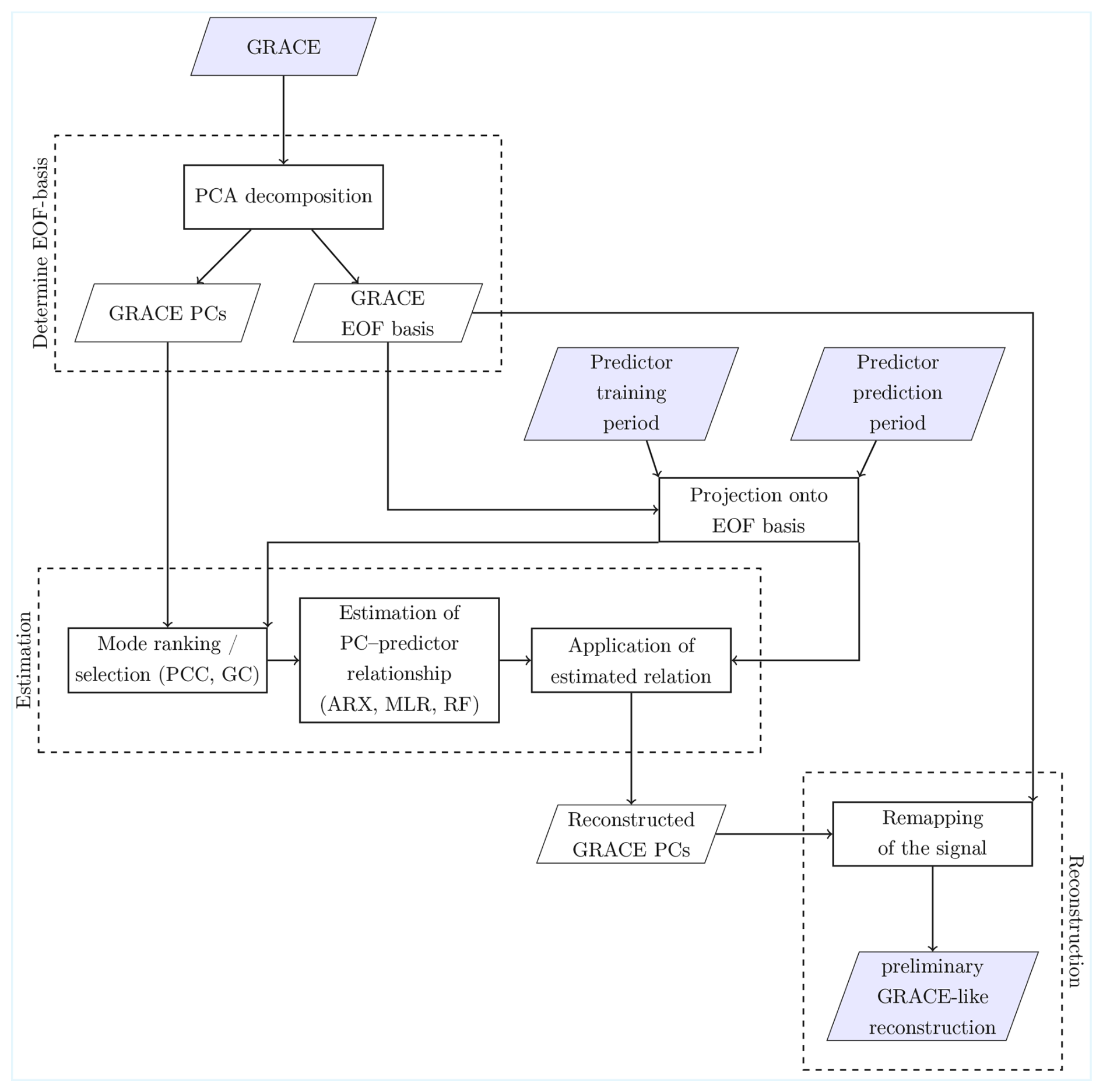
Figure 1 Schematic overview of the framework for the preliminary reconstruction, with the shown processing steps being performed for each basin. The method consists of three stages: (i) the PCA decomposition, in which a reduced EOF basis is derived from GRACE observations; (ii) estimation, where the relationship between projected predictor data and GRACE PCs is identified; and (iii) reconstruction, where the estimated PCs are synthesized to obtain GRACE-like fields. Dashed boxes indicate conceptual grouping rather than execution order.

2.3 Optimal data combination in EOF space

Figure 2 illustrates the schematic overview of the data combination. The common projection of all input data onto the GRACE-derived EOF basis is a key step in the preliminary reconstruction (Fig. 1), enabling the reconstruction to be described within a single orthogonal basis per basin. It provides a shared description of spatial variability, making it easier to relate variations in the predictors to the patterns that drive mass variability observed by GRACE. Additionally, noise and correlations within and between the predictors and the target variables are reduced. We therefore decide to likewise formulate the data combination within a common GRACE-derived EOF basis (Fig. 2) to which we project the preliminary reconstruction and SLR-DORIS data.

The SLR-DORIS data and the preliminary reconstruction are finally combined via variance component estimation (VCE) (Koch, 2018; Förstner, 1979 and Sect. A2). The estimated variance components scale the observation covariance matrix (Eqs. 4 and 10) and can be interpreted as weights among the observation groups contributing to the overall solution. We apply the VCE to the projected PCs and covariance matrices from SLR and the preliminary reconstruction. We set the a-priori variance factor for all data sets to one. Due to the lower resolution of the SLR data compared to GRACE, we aggregate the polygons used for the reconstruction to “super” polygons (Fig. C2). The data combination is performed for every super polygon's first m dominant modes. The number of dominant modes per polygon is illustrated in Fig. C3. The derived variance factors are adjusted by a factor of up to about 10 for SLR and up to about 1000, depending on the mode and basin, for the reconstruction, leading to a higher influence of SLR on the final solution. After deriving and applying the variance components, we remap the adjusted PCs using the GRACE EOF basis (Fig. 2).

We derive variances for TWSTORE by propagating the derived uncertainties of SLR-DORIS and the climate data reconstruction through our combination approach. The averaged standard deviations exhibit uncertainties around 2–6 cm per grid cell. Higher uncertainties are found in regions with greater variability in the TWSA signal (Fig. C5).

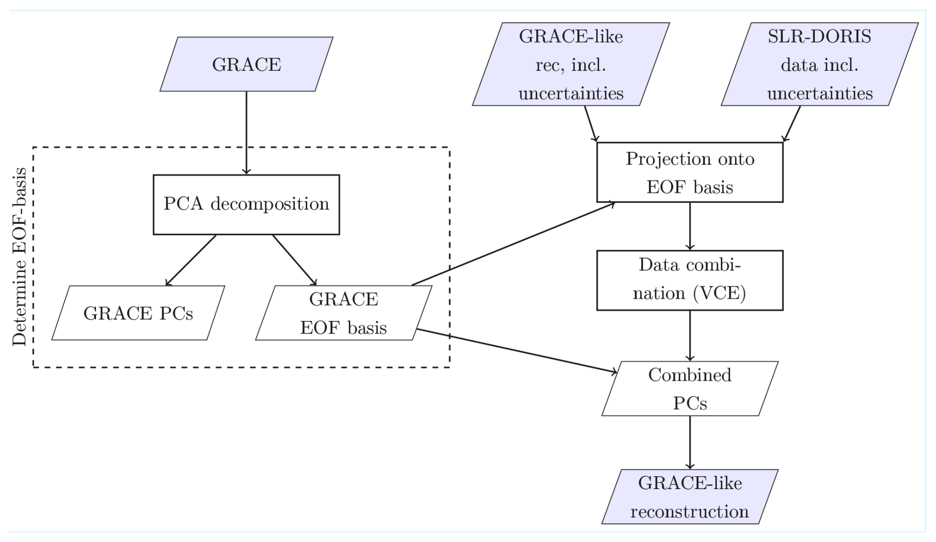
Figure 2 Schematic overview of the framework for the data combination. Dashed boxes indicate conceptual grouping rather than execution order.

2.4 Validation methods

2.4.1 Detecting extreme events using generalized extreme value distribution

Generalized extreme value (GEV) distributions are a family of continuous probability distributions in extreme value theory that combine three classical extreme-value distributions. They are characterized by location, scale, and shape parameters, with the shape parameter governing the tail behavior and thus the probability of rare extremes. The fitted distribution enables sampling, i.e., drawing return values. In the GEV framework, a return level is the quantile of the extreme-value distribution corresponding to a given exceedance probability.

Following Kusche et al. (2016), we derive annual maximum and minimum anomalies of our multidecadal reconstruction of terrestrial water storage per grid cell and fit a Generalized Extreme Value (GEV) function to these time series by using the moment method (Martins and Stedinger, 2000) (see Appendix A4 for the computational details). The anomalies are derived by computing and subtracting the climatology from the reconstruction. We determine the return levels of one in five and one in ten years for extreme anomalous storage conditions. In the given context, the return levels represent the frequency of annual extreme storage surpluses and deficits that exceed average climatological patterns. We then examine whether temporal changes in return levels emerge by partitioning the time frame into overlapping 24-year periods. We focus on annual maximum return surplus and deficit levels for a given return time, as these are sensitive indicators of magnitude increases in the underlying distribution's tails (Allen and Ingram, 2002). It is essential to note, however, that although our reconstruction is based on GRACE and GRACE-FO data, it is not entirely independent of climate datasets and their underlying signal signatures.

2.4.2 Comparison against land water storage from the sea level budget

The global mean sea level budget can be expressed as the sum of steric and mass-driven contributions (Horwath et al., 2022)

$$\begin{array}{}\text{(11)}& {\displaystyle }\mathrm{\Delta }{h}_{\text{GSML}}=\mathrm{\Delta }{h}_{\text{Steric}}+\mathrm{\Delta }{h}_{\text{Mass}}\end{array}$$

assuming the mass component Δh_Mass is already expressed in terms of time-depended sea-level change. The mass component is defined as

$$\begin{array}{}\text{(12)}& \begin{array}{rl}\mathrm{\Delta }{h}_{\text{Mass}}& =\mathrm{\Delta }{h}_{\text{Antarctica}}+\mathrm{\Delta }{h}_{\text{Greenland}}+\mathrm{\Delta }{h}_{\text{Glaciers}}\\ & +\mathrm{\Delta }{h}_{\text{LWS}}+\mathrm{\Delta }{h}_{\text{Other}},\end{array}\end{array}$$

where Δh_LWS represents the influx of water from land (LWS), Δh_Glaciers glaciers outside Greenland and Antarctica, Δh_Greenland the Greenland Ice Sheet and Glaciers, Δh_Antarctica the Antarctic Ice Sheet, and Δh_Other other mass changes, such as variations in atmospheric water content. Assuming that other mass changes, in particular atmospheric water content, are negligible, this leads to

$$\begin{array}{}\text{(13)}& \begin{array}{rl}\mathrm{\Delta }{h}_{\text{GSML}}& =\mathrm{\Delta }{h}_{\text{Steric}}+\mathrm{\Delta }{h}_{\text{Mass}}=\mathrm{\Delta }{h}_{\text{Steric}}\\ & +\mathrm{\Delta }{h}_{\text{Antarctica}}+\mathrm{\Delta }{h}_{\text{Greenland}}+\mathrm{\Delta }{h}_{\text{Glaciers}}\\ & +\mathrm{\Delta }{h}_{\text{LWS}}.\end{array}\end{array}$$

It is obvious from Eq. (13) that water mass changes on land affect the sea level, with a decrease of the water mass on land leading to an increase of the sea level and the other way around. Assuming our reconstruction contains mass changes on land and from Glaciers, a comparison with the GSML change can be facilitated as

$$\begin{array}{}\text{(14)}& \begin{array}{rl}& \mathrm{\Delta }{h}_{\text{Glaciers}}+\mathrm{\Delta }{h}_{\text{LWS}}=\mathrm{\Delta }{h}_{\text{GSML}}\\ & -(\mathrm{\Delta }{h}_{\text{Steric}}+\mathrm{\Delta }{h}_{\text{Steric}}+\mathrm{\Delta }{h}_{\text{Antarctica}}+\mathrm{\Delta }{h}_{\text{Greenland}}).\end{array}\end{array}$$

We use the GMSL products from Frederikse et al. (2020b), covering the period 1901–2018, and from Horwath et al. (2022), spanning 1993–2016. The Frederikse et al. (2020b) data set provides yearly estimates of GSML. For comparison, we thus averaged the other datasets (reconstruction, SLR-DORIS, and GRACE) to a yearly resolution, effectively reducing any seasonal signal. We used the time frame 1984–2018 for the comparison and trimmed all data sets to this period. The data set from Horwath et al. (2022) consists of deseasonalized estimates of GMSL on the monthly scale, and here we removed the seasonal signal in the other data sets via a least-squares adjustment for mutual consistency. Both GMLS data products provide the components of the sea-level budget equation that we used here to infer land water storage change.

2.4.3 Terrestrial water budget

Given that multidecadal time series for measured precipitation and river discharge exist for several river basins, it is tempting to evaluate the terrestrial water budget with the reconstructed terrestrial water storage records and solve for basin-averaged evapotranspiration, as done, e.g., earlier in several studies for the GRACE/-FO period (e.g., Xiong et al., 2023). The term “evapotranspiration” (Miralles et al., 2020) refers to the total freshwater flux between the atmosphere and the surface through all types of evaporation and condensation, including those from transpiration and interception by vegetation, sublimation, and deposition, where downward fluxes are defined as positive. Evapotranspiration plays a crucial role in the water and energy cycles, as it is sensitive to climate change and anthropogenic land-use changes, providing insight into the history of the land surface's response to various forcings. Several studies suggest that global evapotranspiration might have changed significantly at decadal timescales (Douville et al., 2013), both due to changes in evaporative demand (temperatures) and moisture supply (vegetation, rainfall), but direct (flux-tower) measurements are scarce. Independent data sets from the budget approach can also aid in evaluating meteorological reanalyses (e.g., Springer et al., 2014).

We therefore decided to evaluate basin-averaged monthly evapotranspiration $\stackrel{\mathrm{‾}}{\mathrm{ET}}$ for eleven major river basins of the world located in different climate zones, with a focus on the Amazon, the Niger, and the Danube basin. We use the formulation of the terrestrial water budget (where σ equals TWSA, as above)

$$\begin{array}{}\text{(15)}& {\displaystyle \frac{\mathrm{d}\mathit{\sigma }}{\mathrm{d}t}}=P-\mathrm{ET}-R\end{array}$$

with precipitation P and river discharge R, which is rearranged for evapotranspiration ET and is numerically evaluated as in Springer et al. (2014). For terrestrial water storage changes $\mathrm{d}\mathit{\sigma }/\mathrm{d}t$, we use TWSTORE via bare first-order central differences without filtering. We use the GPCC 2022 dataset for precipitation, as shown in Table 2. River discharge is obtained from the Global Runoff Data Center (GRDC), Koblenz. All data sets span the period from 1984 to 2020, except for the Igarka (Yenisey) discharge, which ends in 2017 (cf. Table B2). In addition, we compare the derived $\stackrel{\mathrm{‾}}{\mathrm{ET}}$ with evaporation from GLEAM (Miralles et al., 2025) and ERA5 (Hersbach et al., 2020) after temporal binning and averaging over the basin area. Furthermore, we also computed a budget-derived $\stackrel{\mathrm{‾}}{\mathrm{ET}}$ version in which P is replaced with ERA5 total precipitation. Offsets and trends of the monthly resolved time series are estimated using a six-parameter least-squares adjustment, which includes an offset, a linear trend, and semi-/annual component terms. For a direct quantitative comparison of seasons-retaining $\stackrel{\mathrm{‾}}{\mathrm{ET}}$ series, we compute Pearson correlation coefficients over their common period. The derived time series for evapotranspiration are available at https://doi.org/10.5281/zenodo.16643628 (Gutknecht, 2025).

3 Data

Three data types are important for this study: GRACE data, the climate data used as predictors, and the SLR-DORIS data. The GRACE level-2 data are converted to TWSA maps. They serve to generate the EOF bases, in which the outcome of the preliminary reconstruction and the SLR-DORIS data are represented and combined, and for training the preliminary reconstruction in Sect. 2.2. After describing the GRACE postprocessing, we summarize the climate data and the SLR-DORIS data set used in this study.

3.1 GRACE products

Peltier et al. (2015)Kvas et al. (2019); Mayer-Gürr et al. (2018b)Peltier et al. (2015)Jäggi et al. (2022)Peltier et al. (2015)Loomis et al. (2019)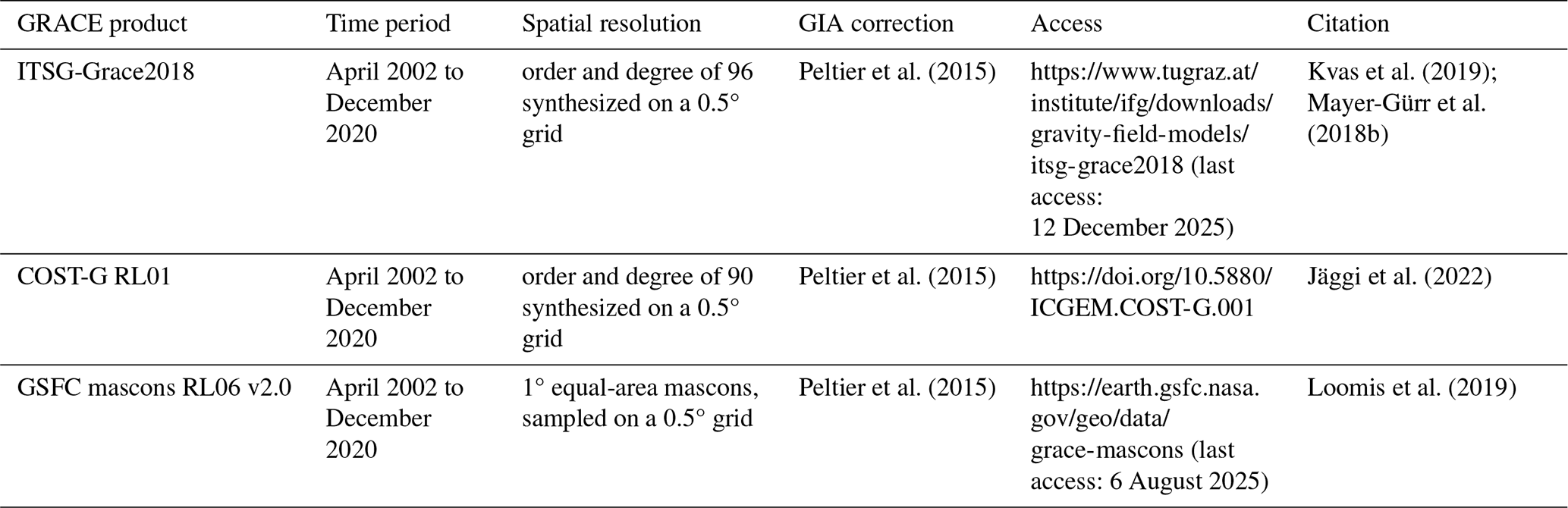

Table 1 Overview of used GRACE products.

In this study, we used three different GRACE solutions: monthly ITSG-Grace2018 gravity fields computed at Graz University of Technology (Kvas et al., 2019; Mayer-Gürr et al., 2018b) of order and degree 96 for the years April 2002 to December 2020, the International Combination Service for Time-variable Gravity Fields (COST-G) RL01 solution from the University of Bern (Jäggi et al., 2022) of order and degree 90 for the years April 2002 to December 2020 and the NASA GSFC global mascon product on a 0.5×0.5° grid (Table 1). For the two L2 products (ITSG-Grace2018 and COST-G), we reduced the temporal mean from 2003 to 2020 from the spherical harmonics (geopotential) coefficients. We replaced the degree 1 and c₂₀ coefficients with those from NASA/JPL (Cheng and Ries, 2023; Swenson et al., 2008), as GRACE measures these coefficients poorly. Following Loomis et al. (2020), we also replaced the c₃₀ coefficient for the late GRACE months, compensating for the degrading estimates from GRACE due to accelerator problems. The coefficients were smoothed with the anisotropic DDK3 filter (Kusche, 2007; Kusche et al., 2009) to reduce the noise level of the GRACE-derived coefficients. The post-glacial rebound (glacial isostatic adjustment (GIA)) of the Earth causes a redistribution of interior Earth mass, leading to a long-term gravity trend unrelated to water storage variations. The effect of GIA was removed from the coefficients. We synthesized the gravity fields (Wahr et al., 1998) from the coefficients on a 0.5×0.5° grid and interpolated missing months using Akima Spline interpolation. It should be noted that the actual resolution of GRACE is much coarser (around 330 km at the equator) and is not reflected by the grid (around 55 km for a 0.5° grid) (Humphrey et al., 2023).

3.2 Climate data

We used five different predictors, all of which were provided in gridded fields. Two of these predictors were related to water cycle variables (precipitation, P, and soil moisture, SM), two to the energy cycle (sea surface temperature, SST, and air temperature, T), and one to the carbon cycle (leaf area index, LAI).

SST and SM influence atmospheric moisture and heat transfer. The variables are closely connected to evapotranspiration rates and rainfall. High SST values lead to high air moisture content and heavy rainfalls, which can cause floods. SM determines plant water availability, which in turn influences plant growth and CO₂ uptake. Low SM values can indicate droughts, whereas high soil moisture contents can cause higher runoff rates and possibly floods. T is the driver for the movement of water masses, influencing the phase changes of water (evaporation, condensation, freezing) and energy fluxes. P patterns determine regional climates and ecosystems, replenishing freshwater supplies and maintaining SM. Like SM, P is linked to droughts and flood events. LAI is an indicator of water uptake by plants, evapotranspiration, and photosynthesis, which connects the water cycle to the carbon cycle.

We refrain from including climate indices here. Although they have been helpful in studies aimed at optimizing prediction skills, they are compounded by the variables mentioned, and we expect them to obscure our causality framework. Moreover, some are derived directly from SST.

The data sets used in this study are listed in Table 2. We use two datasets for SST, P, and SM and one dataset for T and LAI. For SST, we utilized the Met Office Hadley Centre's sea ice and sea surface temperature (SST) dataset, HadISST1, and the COBE-SST 2 and Sea Ice dataset provided by the National Oceanic and Atmospheric Administration (NOAA) Physical Sciences Laboratory (PSL). HadiSST is global monthly averaged SST anomalies derived from in situ ship-based measurements, drifting and moored buoys, and satellite observations. HadISST1 employs interpolation techniques and statistical methods to fill data gaps. COBE-SST 2, in contrast, does not include satellite observations. The data set focuses on in situ data. SST values are interpolated by minimizing the differences between observed and reconstructed SST values. For precipitation, we utilize the Global Precipitation Climatology Centre (GPCC) dataset, operated by the German Meteorological Service (Deutscher Wetterdienst, DWD), and the Climate Prediction Center's (CPC) Global Precipitation V1.0 Data Set, provided by NOAA. The GPCC data set is based on in situ observations from over 85 000 rain gauges worldwide, provided by national meteorological and hydrological services (NMHSs), global data collections (e.g., SYNOP), and research networks. The CPC data set, provided by NOAA, combines in situ gauge-based precipitation observations with satellite-derived precipitation estimates. The CPC soil moisture data set is not directly measured but rather modeled using a water balance model that incorporates precipitation data from NOAA's CPC Unified Precipitation dataset and temperature inputs from NCEP-NCAR reanalysis data. GHCN CAMS Monthly Temperature data are derived from in situ observations from surface weather stations that report to the Global Historical Climatology Network (GHCN). Globmap LAI v3 is based on satellite observations using data from sensors such as the AVHRR (Advanced Very High-Resolution Radiometer) (pre-2000) and MODIS (Moderate Resolution Imaging Spectroradiometer) (after 2000).

Rayner et al. (2003)Hirahara et al. (2014)Schneider et al. (2022)Chen et al. (2008)Fan and van den Dool (2004)Miralles et al. (2025)Fan and van den Dool (2008)Liu et al. (2012)

Table 2 Overview of the climate data sets used in the preliminary prediction.

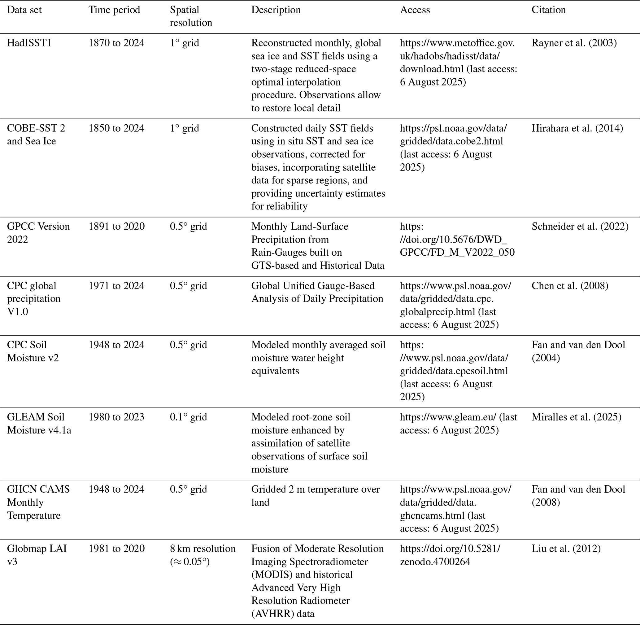
All data sets were trimmed to the period 1984–2020, averaged or summed to monthly data, and, except for the SST data, resampled to a 0.5° grid. SST data were not resampled as the variable is part of the far-field variables. Missing data points (due to different land masks between GRACE and the predictors) are interpolated.

3.3 Large-scale gravity fields from SLR and DORIS

In this study, we utilize the solution proposed by Löcher et al. (2025b). The dataset is a combination of satellite laser ranges from six satellites and ten satellites tracked by Doppler Orbitography and Radiopositioning Integrated by Satellite (DORIS). For pre-1992 full-rate laser ranging data, normal points were formed as described in Löcher et al. (2025b). The range rates derived from the Doppler observations were integrated into biased ranges. The observations were combined at the level of the normal equations and solved on the basis of the EOF derived from GRACE. Eventually, the results were subsequently converted to SHC complete to degree and order 60.

4 Evaluation of the combined reconstruction

Following, we will assess the impact of the combination procedure by comparing it to the SLR-DORIS and preliminary climate data reconstructions. Afterward, we compare terrestrial water storage maps from GRACE-FO, which was not used in the training process, and finally, we compare our reconstruction, TWSTORE, with other published reconstructions. TWSTORE and associated uncertainties are available as NetCDF at https://doi.org/10.5281/zenodo.15827789 (Hacker, 2025).

4.1 Impact of the data combination

Our terrestrial water storage reconstruction is, to our knowledge, the first attempt to integrate satellite-geodetic records with data-based methods. In this section, we therefore assess the impact of the data combination (Sect. 2.3).We analyze the trend, acceleration, annual amplitude and phase, inter-annual, and sub-seasonal signal for 1984–2020 for the preliminary reconstruction from climate data without integrating SLR-DORIS (REC w/o DC), the SLR-DORIS solution (SLR-DORIS), and the combined reconstruction (TWSTORE) (cf. Fig. 3 and Table 3; see Hacker and Kusche, 2024 for computational details on the metrics). We expect that the influence of the satellite-geodetic data set will vary by region, as its weight in the combination is controlled by both the uncertainty description of the SLR-DORIS covariance matrix and the ensemble of the preliminary reconstruction.

The SLR-DORIS TWSA fields exhibit strong signal magnitudes across all metrics (Table 3 and Fig. 3). In comparison, the preliminary reconstruction exhibits notably smaller amplitudes, in particular for the trend and acceleration (Fig. 3). It is notable that the trend rate and acceleration in our reconstruction (TWSTORE) are controlled by the SLR-DORIS solution, with water storage change from SLR-DORIS having magnitudes up to three (and more) times larger than the preliminary reconstruction (Table 3) and the metrics of TWSTORE leaning towards those of SLR-DORIS.

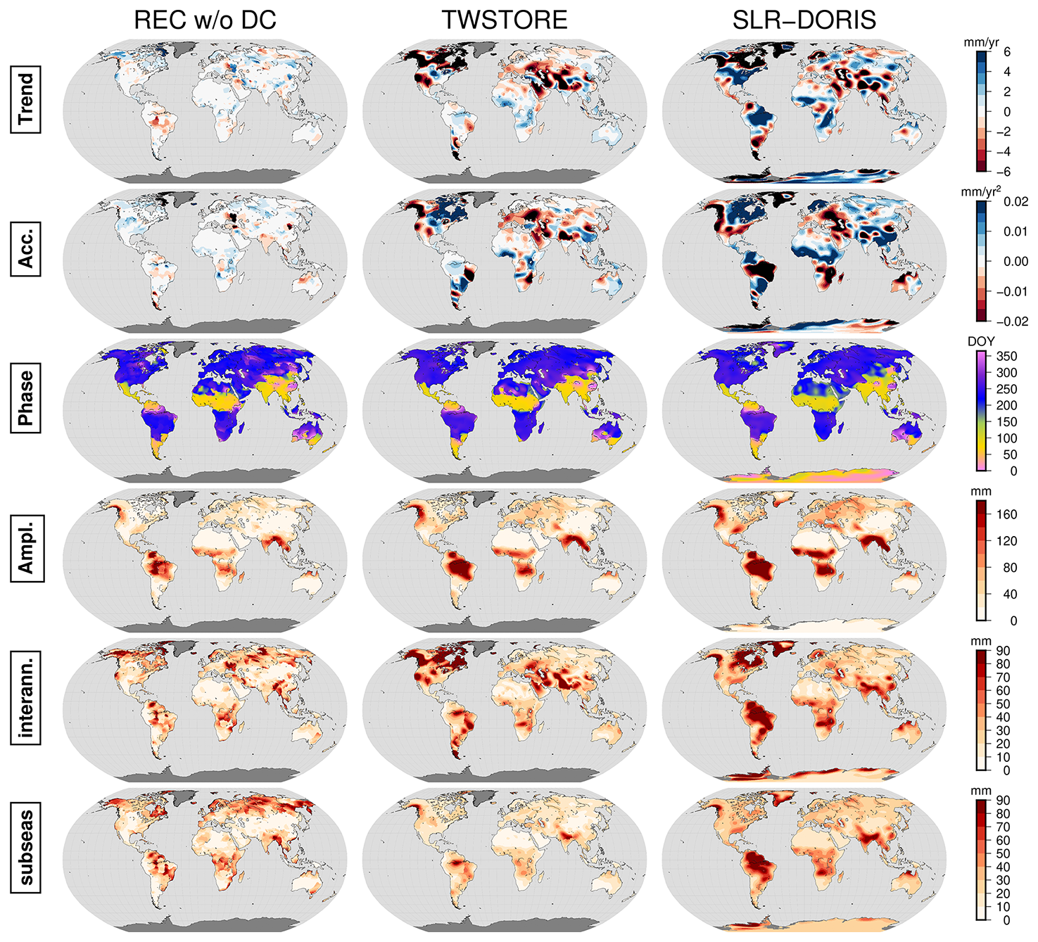
Figure 3 Trend, acceleration, annual amplitude and phase, interannual and subseasonal signal of the preliminary reconstruction (without data combination (DC)), TWSTORE and the SLR-DORIS fields for a spherical harmonic degree of n=60.

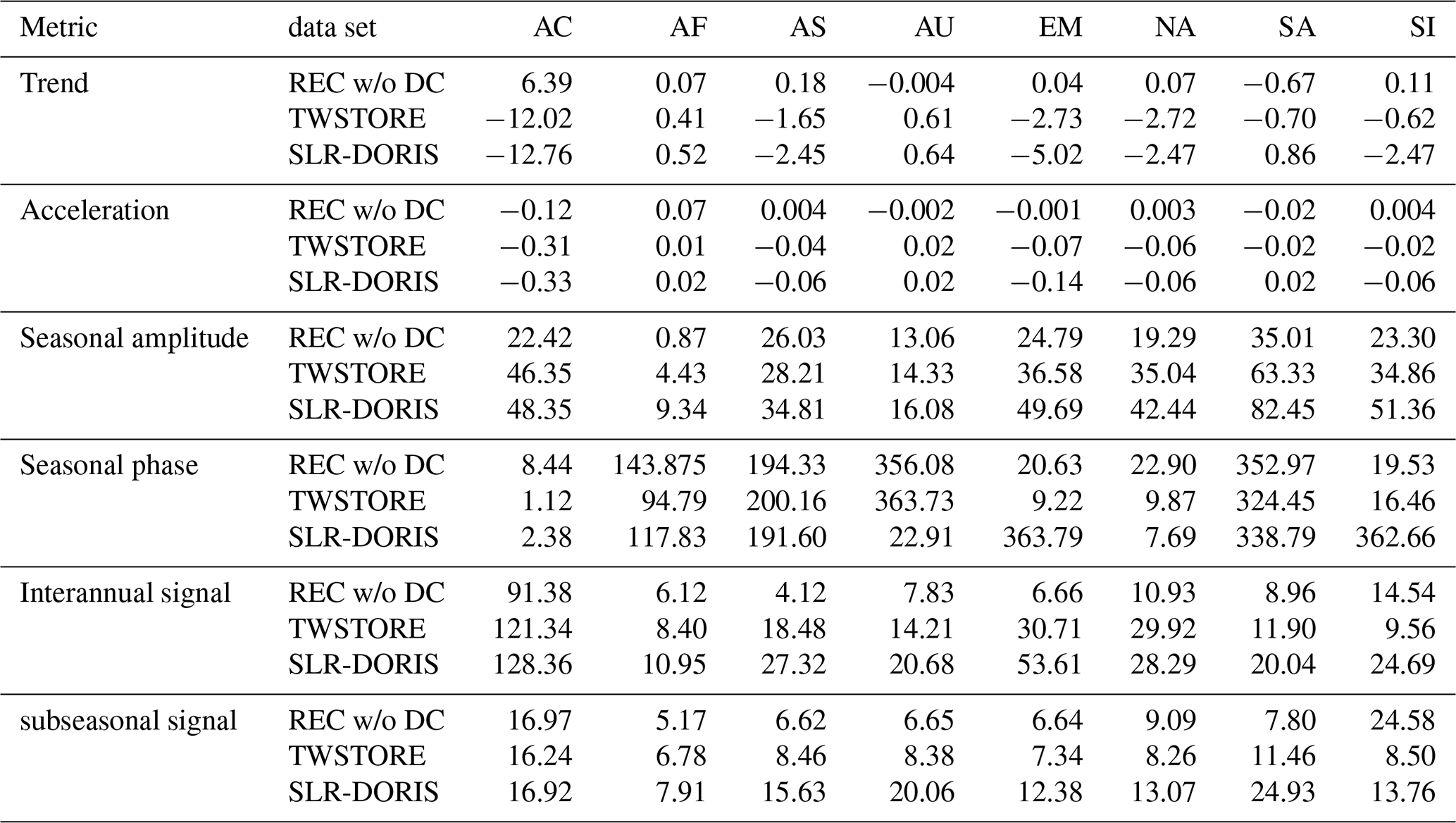
We decided to evaluate our three solutions for terrestrial water storage change across the major continental regions of the world, where recent studies based on GRACE data have revealed major losses on all continents except Africa (Rodell et al., 2024; Zhang et al., 2025; Chandanpurkar et al., 2025). As mentioned above, we find stark differences between the geodetic (i.e., SLR and DORIS) and the climate reconstruction solution. A prominent example is the Arctic region of Alaska and northern Canada (AC in Table 3). For this region, the preliminary reconstruction exhibits a trend of 6.39 mm yr⁻¹ and an acceleration of 0.12 mm yr⁻². In contrast, SLR-DORIS shows a trend of −12.76 mm yr⁻¹ and an acceleration of 0.33 mm yr⁻². The combined product then, clearly influenced by the SLR-DORIS solution, reveals a trend of −12.02 mm yr⁻¹ and an acceleration of 0.31 mm yr⁻². Similar influences of the SLR-DORIS data on TWSTORE can be found for Asia (AS), Australia (AU), Africa (AF) and the central part of North America (NA). This effect is desired since the tracking data should be superior to climate data reconstruction at these timescales. It is essential to note that the weighting between climate-driven and geodetic reconstruction is determined by the ensemble uncertainty of the preliminary reconstruction in comparison to the SLR-DORIS uncertainty, and this uncertainty varies by basin. The influence of the SLR-DORIS data onto TWSTORE is also clearly visible for the seasonal, interannual and subseasonal signals (AC, AS, AF, AU, and EM in Table 3). An exception is South America, where the interannual and subseasonal signal of TWSTORE leans toward the preliminary reconstruction, possibly influenced by high uncertainties in the SLR-DORIS data in the Amazon basin. Unexpected is the reduction in interannual and subseasonal signal magnitude of TWSTORE for Siberia, with the interannual signal magnitude of 9.56 mm for TWSTORE, compared to 24.69 mm (SLR-DORIS) and 14.54 mm (preliminary reconstruction). For the subseasonal signal magnitude, the derived magnitude is 8.5 mm, compared to 13.76 mm (SLR-DORIS) and 24.58 mm (preliminary reconstruction). However, the subseasonal signal in the preliminary reconstruction is dominated by several outliers (not shown), leading to an overall high magnitude. Due to the data combination, those signal jumps are not transferred to the final data product. It is also worth noting that the SLR-DORIS contribution led to higher uncertainty from 1984 to 1992, as these observations were noisier during this period (Löcher et al., 2025b).

Table 3 Trend, acceleration, seasonal amplitude, and phase, magnitude of the subseasonal and interannual signal for different continents and subcontinents: AC: Arctic northern Canada, AF: Africa, AS: Asia, AU: Australia; EM: Europe and Middle East, NA: (central) Northern America, SA: South America, SI: Siberia (see Fig. C4) for SLR-DORIS, the preliminary reconstruction and TWSTORE for 1984–2020. Trend, acceleration, annual amplitude, and phase were estimated in a four parameter least squares adjustment, subseasonal and interannual signal were determined by using a low/high pass filter on the time series. Trend: mm yr⁻¹, acceleration mm yr⁻², seasonal amplitude mm, seasonal phase DOY, magnitude of the interannual and subseasonal signal mm.

4.2 Comparison against GRACE/-FO (2002–2020)

We first compare the reconstruction with terrestrial water storage anomalies from the GRACE mission. However, this cannot be considered an independent evaluation, as our preliminary reconstruction was trained using the GRACE data. Nevertheless, comparing the performance of the reconstruction with both GRACE and GRACE-FO provides an impression of the reconstruction's prediction skill.

Figure 4 illustrates the root mean square deviation (RMSD) between the reconstruction and GRACE/-FO terrestrial water storage. We find lower skills and higher RMSD values up to 200 mm in Alpine and highland regions, which we attribute to the reconstruction's limited ability to describe TWSA in the presence of glacier and snowpack changes. Compared to GRACE-FO, high RMSD values up to 200 mm are observed in the regions around the Great Lakes of North America and Alaska. The high values in North America could indicate a mismatch in the GIA correction, but this requires further investigation. However, the RMSD values for Fennoskandia and Northern Europe are quite small, with values ranging from 20–60 mm. Notably, lower predictive skills are also observed for Turkey, the region around the Caspian Sea, the Volga-Don River, and the area around the Aral Sea. We suspect this may be due to anthropogenic effects, such as damming activities or irrigation with river water, which are not, or are only partially, represented in the reconstruction. We find RMSD values of around 120–180 mm between the reconstruction and GRACE-FO for certain aquifers that experience (accelerated) groundwater decline (Jasechko et al., 2024), such as the North China Plain, the Middle Chao Phraya basin, the Lower Zayandeh-Rud basin, and the Southern High Plains. The mismatch is probably due to our preliminary reconstruction not accounting for the accelerated declines in TWSA, which were less severe during the training period.

Figure 5 shows the Pearson correlation coefficient between the detrended and deseasonalized data sets, specifically TWSTORE vs. GRACE (January 2003–December 2016) and TWSTORE vs. GRACE-FO (July 2018–December 2020). We generally find lower correlations for arid and highland climate regions with correlation coefficients ranging from −0.2 to 0.4 against GRACE and −0.4 to 0.8 against GRACE-FO. The low correlation may be attributed to the small TWSA signal and the inability of the predictors, primarily precipitation, soil moisture, and leaf area index, to represent the changes in TWSA in these regions accurately. On the other hand, for areas with a humid climate, we find a high correlation up to 0.9. As might be expected, advancing the reconstruction to the more recent GRACE-FO data results in a loss of correlation compared to GRACE, most pronounced in Australia (0.4–0.8 for GRACE to −0.4 to 0.6 for GRACE-FO), the Amazon basin, the region around the Caspian Sea, and the Sahara. Although not optimal, a slight phase shift can be expected when predicting a time series.

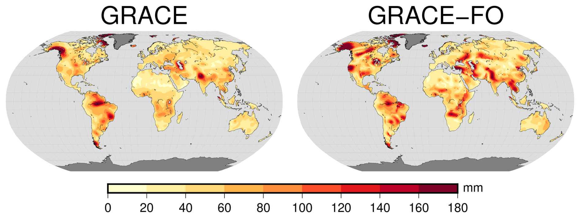
Figure 4 Root Mean square deviation between GRACE/-FO and the reconstruction.

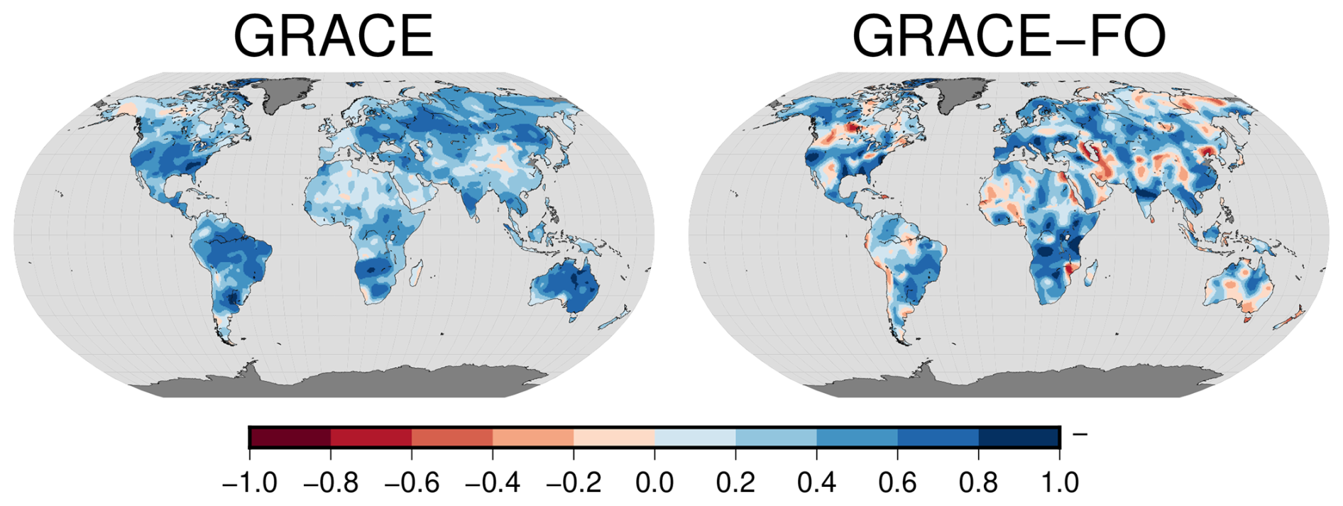
Figure 5 Correlation (of deseasonalized, detrended anomalies) between GRACE/-FO and the reconstruction.

4.3 Comparison to other reconstructions

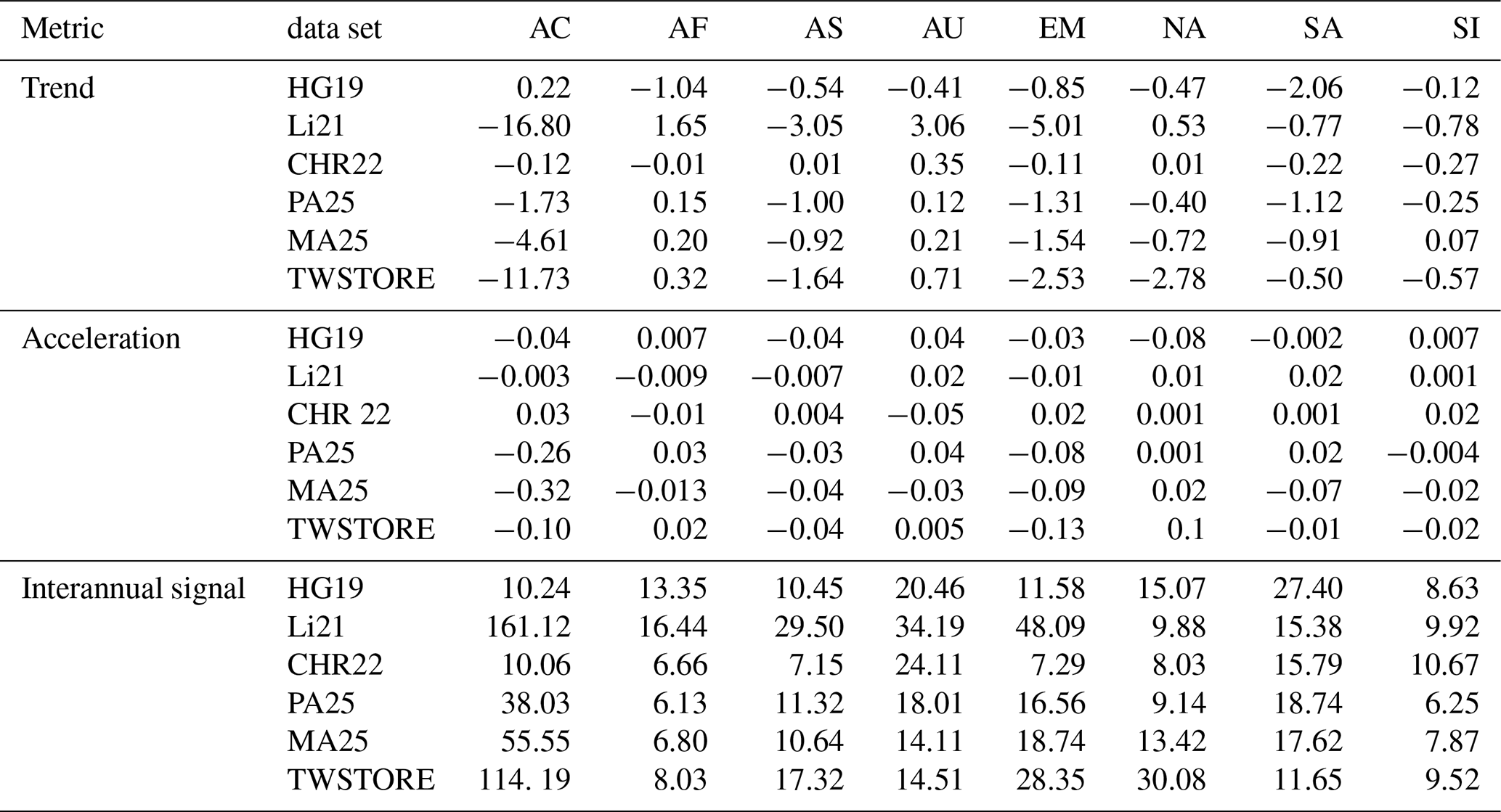
A comparison with GRACE data provides limited insight into the reconstruction's performance, as it cannot be considered an independent dataset. Point-wise validation data are also impractical due to the reconstruction resolution, and the SLR data from Löcher and Kusche (2021) is not independent either. Therefore, we compare our reconstruction with other GRACE-like TWSA reconstructions. The comparison with other reconstructions can be seen as an internal evaluation that assesses consistency across different data sets. The employed reconstructions differ in the data sets used and the reconstruction principles (Humphrey and Gudmundsson, 2019b; Li et al., 2021; Chandanpurkar et al., 2022b; Palazzoli et al., 2025; Mandal et al., 2025). Hacker and Kusche (2024) evaluated the reconstructions by Humphrey and Gudmundsson (2019b); Li et al. (2021); Chandanpurkar et al. (2022b) and found a high agreement of the reconstructions for the seasonal and subseasonal signals, as those signals are quite dominant and easily identified by learning algorithms. We found similar agreement for our reconstruction, to the ones used in the study of Hacker and Kusche (2024), and the ones from Palazzoli et al. (2025); Mandal et al. (2025). Therefore, we focus on the long-term signals, namely: trend, acceleration, and interannual signals, and derive them from the reconstructions for 1984–2019 (Fig. 6). Similar to Sect. 4.1, we compute the selected metrics for the same (sub) continents (Table 4). It is important to note that the reconstruction by Humphrey and Gudmundsson (2019b) focuses on the inter-annual signal and does not include a trend. The reconstruction by Li et al. (2021) incorporates the trend derived from GRACE in the training period. However, as demonstrated in Hacker and Kusche (2024), the statistical model used by Humphrey and Gudmundsson (2019b), in combination with the employed predictors, yields a signal component that, based on a least-squares adjustment, is identified as a trend.

From Fig. 6, the reconstructions agree on negative trends in regions affected by (historical) droughts, like the US and the Arabian Peninsula, regions affected by ice mass loss, e.g., Siberia and the Andes, and regions affected by water loss due to anthropogenic effects, such as the region around the Caspian Sea and Aral Sea. However, as shown in Table 4, the magnitude of the derived trend differs notably across regions. For example, for Europe and the Middle East (EM in Table 4), the computed trends range from −5.01 mm yr⁻¹ (Li21) to −0.11 mm yr⁻¹ (CHR22). In Alaska and northern Canada, HG19 even indicates a positive trend of 0.22 mm yr⁻¹, whereas the other reconstructions show trends ranging from −16.8 mm yr⁻¹ (Li21) to 0.12 mm yr⁻¹ (CHR22). The strong trend of Li21 originates from the GRACE-based trend, which is added to the reconstruction instead of directly reconstructed (Li et al., 2021). Notable differences arise in the Amazon basin, Africa, and China. The corresponding metrics in Table 4 exhibit differences in magnitude and sign. We hypothesize that these differences are due to dynamic processes, partly influenced by humans, that are not well captured in the predictors of the reconstruction. However, the trends derived from the different reconstructions reveal a decrease in TWSA across most (sub)continents, indicating that decreasing TWSA rates were already underway in the pre-GRACE period. The positive trend in Australia observed across all reconstructions except HG19 is mainly due to the strong La Niña event in 2011 (Boening et al., 2012), which dominates the time series. From Fig. 6, our reconstruction appears to exhibit the strongest accelerations in terms of signal magnitude, which originate from SLR. However, from Table 4, it is clear that our reconstruction shows strong accelerations in hotspot regions, such as the Don basin and the Gulf of Alaska, but does not exhibit the strongest signal magnitudes for (large) area averages. As for the trend, the reconstruction-derived acceleration differs in both magnitude and sign, especially for Australia (AU, −0.05 mm yr⁻² (CHR22) to 0.04 mm yr⁻² (HG19 and PA25)) and Siberia (SI; −0.02 mm yr⁻² (TWSTORE) to 0.02 mm yr⁻² (CHR22)). Except for HG19, all reconstructions were trained on a short training period within the GRACE period. The brief training period makes it challenging to recover interannual signals, such as acceleration, contributing to the variability in the signal magnitude and sign observed here. Similar to the findings for acceleration, the interannual signal shows the greatest variation in magnitude and pattern across the datasets. The data sets agree on high inter-annual signal variations in the Amazon Basin and along the Atlantic coast of South America, the Zambezi Basin, the region around the Don Basin, and India (Fig.  6). Except for Siberia, South America, and central North America, Li21 exhibits the most substantial interannual signal magnitude (Table 4). As shown in Fig. 6, regions with strong trends and high interannual signal magnitudes are closely related for Li21, leading to the conclusion that, once again, the GRACE-derived trend of Li21 is the culprit for the high signal magnitudes found here. In terms of signal magnitude, our reconstruction is well within the range of the derived values from the other reconstructions. An exception is South America, where TWSTORE exhibits the smallest signal magnitude with 11.65 mm compared to 27.4 mm (highest signal magnitude; HG19). The small magnitude is related to a surprisingly small signal in the Amazon basin.

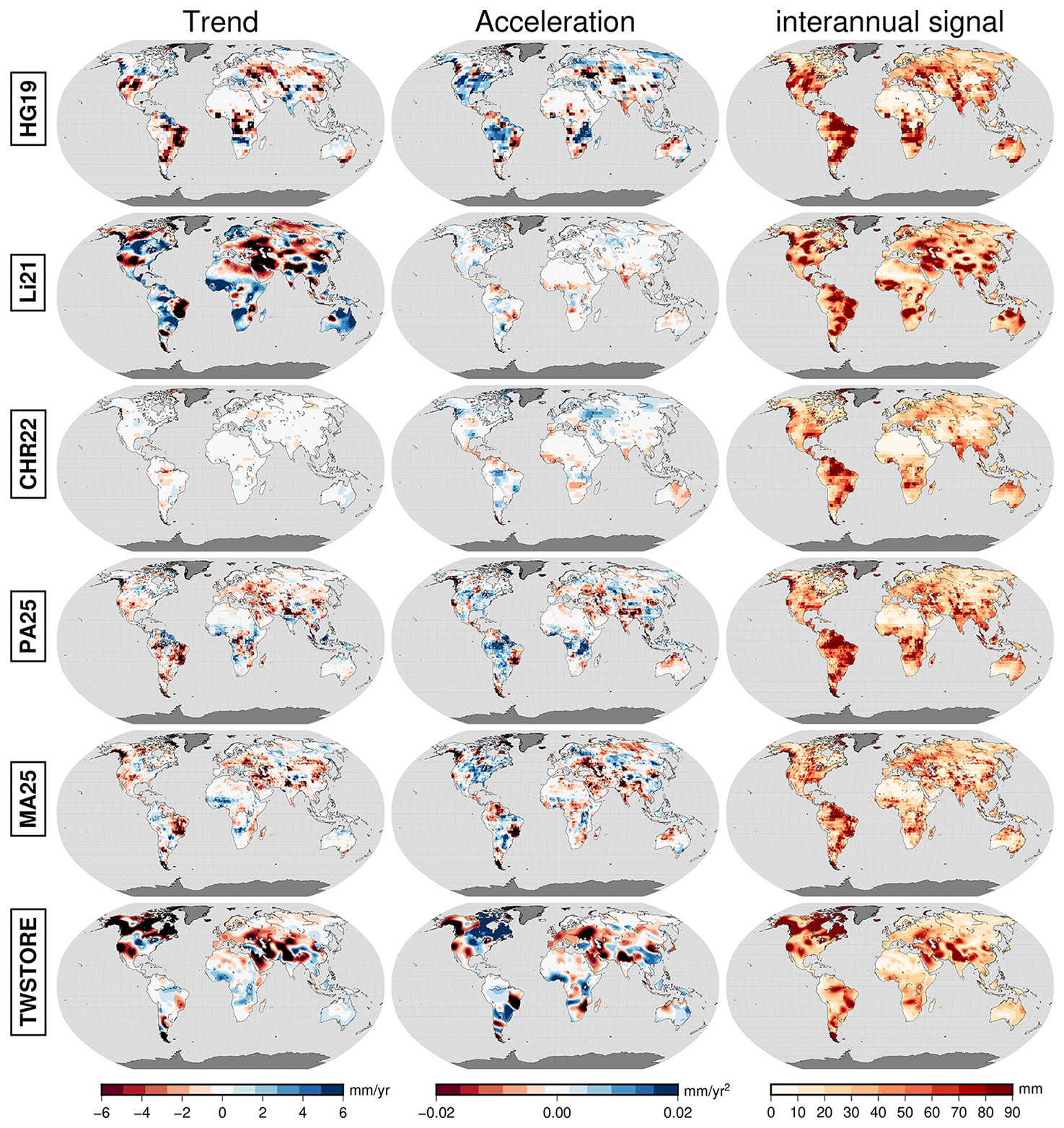
Figure 6 Trend, acceleration, annual amplitude and phase, sub-seasonal and inter-annual signal for HG19, Li21, CHR22, PA25, MA25 and TWSTORE for 1984–2019 on a global scale.

Table 4 Trend, acceleration and the magnitude of the interannual signal for different continents and subcontinents (see Fig. C4) for the selected reconstructions and TWSTORE for 1984–2019. Trend, and acceleration were estimated in a four parameter least squares adjustment (including the seasonal components, not shown here), interannual signal were determined by using a low pass filter on the time series. Trend: mm yr⁻¹, acceleration mm yr⁻², magnitude of the interannual signal mm.

5 Results

5.1 How often did extreme terrestrial water storage deficit or surplus occur during the past decades?

Due to the still short GRACE/-FO data record, only a few studies (Moore and Williams, 2014; Humphrey et al., 2016; Kusche et al., 2016) have assessed the statistics of extreme TWSA events, i.e., beyond analyzing either episodic droughts and floods, or the second moments of the underlying probability distribution. It is an open question whether the expected intensification of the water cycle due to global warming (Huntington, 2006; Durack et al., 2012) has already been observed in space gravimetry and if yes, whether it can be attributed to climate drivers. For example, Yoon et al. (2015) project an increase in the variance of California top-1 m soil moisture by at least 50 % towards the end of the 21st century.

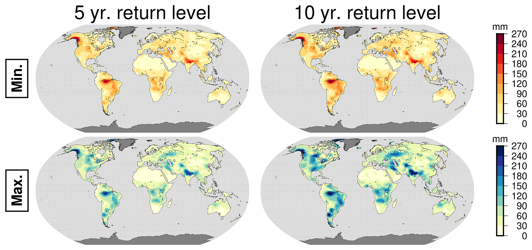
Figure 7 One-in-five-year and One-in-ten-year return levels of anomalously low (top) and high (bottom) terrestrial water storage (TWS) with respect to climatology for different reconstructions for 1984–2020.

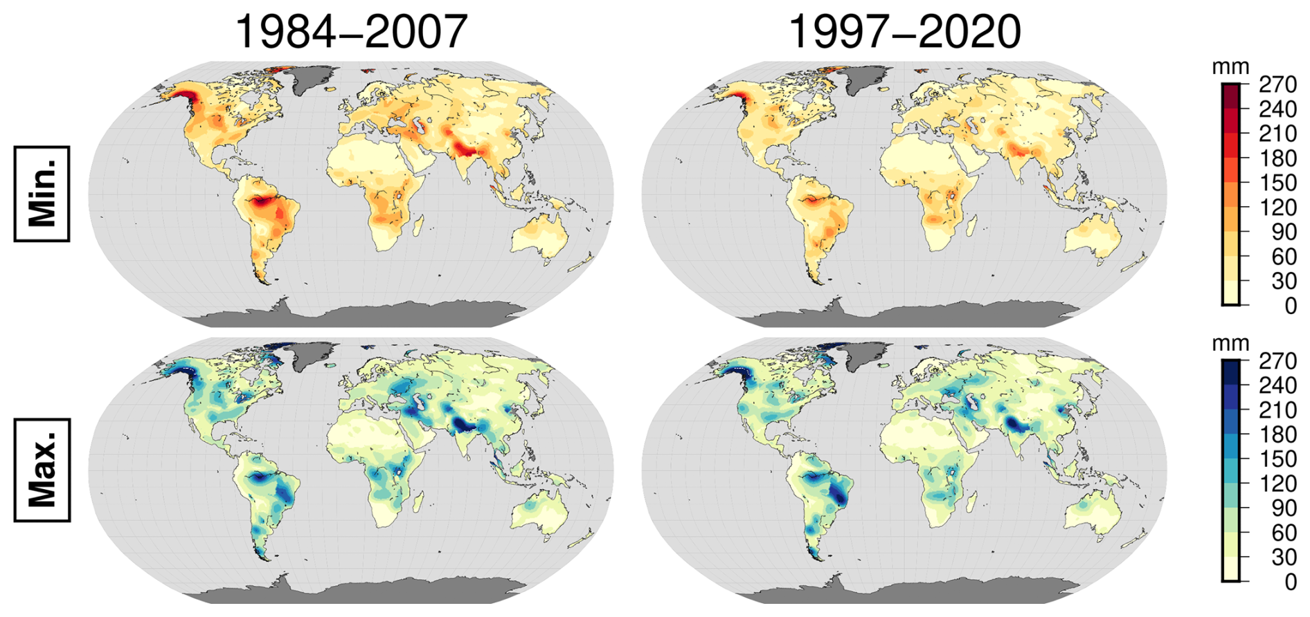
Figure 8 One-in-five-year return levels of anomalously low(top) and high (bottom) terrestrial water storage (TWS) with respect to climatology for two 24-year periods 1984–2007 and 1997–2020.

Figure 7 demonstrates that, due to droughts and rainfall extremes over the last few decades, a one-in-five-year storage deficit (surplus) has reached 20–30 cm below (above) the climatological conditions for some of the major river basins. In contrast, at the one-in-ten-year scale, this could be 60 cm (in the Amazon basin). We expect that extreme storage surplus or deficit primarily reflects rainfall patterns, and we speculate that the signal characteristics might change with the specific choice of predictors, precipitation, and temperature. As expected, due to its strong TWSA signal, driven by high precipitation and influenced by ENSO, which leads to droughts and floods, the Amazon basin is identified here as the global hotspot, with the highest (up to 0.3 m) and lowest (0.3 m) one-in-five-year return levels. Additionally, the reconstruction indicates peak annual anomalous surpluses and low water storage levels for the Zambezi Basin, the Congo Basin, and the region surrounding Lake Victoria. High return levels are also identified for the Orinoco, Essequibo, São Francisco, and La Plata/Paraná river basins. We find moderate return storage levels for the US, primarily in the Mississippi Basin, the region surrounding the Caspian Sea, and the Volga-Don Basin. Figure 1 in Kusche et al. (2016) shows peaks and lows at the one-in-five-year level for the GRACE data from 2003–2015, the corresponding time series, and the empirical and fitted probability density functions. When compared to Fig. 1 in Kusche et al. (2016), we observe close similarities in the spatial patterns of the one-in-five-year levels, with signal peaks in the Central Amazon and the Mississippi basin, and low events being concentrated in the Amazon and the Zambezi basin. Our return levels are found somewhat lower than those reported in Kusche et al. (2016). However, this is an expected outcome as we here analyzed water storage anomalies with respect to a multi-decadal climatology of a reconstruction trained on more recent GRACE data, whereas in Kusche et al. (2016), only 12 years of data were available. Spatial patterns of one-in-five and one-in-ten year extremes are similar, of course, since both one-in-five and one-in-ten year return level maps are based on the same estimates for the GEV distribution parameters.

Lastly, to identify temporal changes, we divided our water storage reconstruction into two overlapping 24-year periods. For consistency, we derive return levels for the annual water storage surplus and deficit concerning the same long-term climatology. As the sliding window overlaps by about 50 %, the results cannot be entirely independent. However, shortening the analysis window further would result in a loss of robustness for the moment estimates, as shown by simulations in (Kusche et al., 2016).

We find for most regions somewhat higher return levels for storage deficits for the 1984–2007 timeframe compared to the more recent period, which at first glance seems counterintuitive in light of the narrative of more severe and more frequently occurring drought conditions. However, return levels express the magnitude of a hypothetical anomalous event that occurs under a given probability relative to the mean storage. In other words, our analysis tells that the variability of annual minimum storage conditions with respect to the long-term mean was higher from 1984 to 2007 than in recent years. Fluctuations in yearly water storage lows in recent years were less pronounced. However, this should not be confused with the magnitude or duration of the recent annual water storage deficit, which contributed to an observed multi-decadal decrease in water storage. These storage trends have been found to bias the computation of drought indicators, as these typically rely on the assumption of nonstationarity (Gerdener et al., 2020).

In contrast, we find only a few differences between the two time frames when comparing the return levels for extreme water storage surplus. A visual inspection suggests that return levels have been larger in the Amazon, Zambezi, and East African Rift Valley from 1984 to 2007 compared to 1997–2020. In contrast, in the La Plata/Paraná and, for example, the North China Plain, return levels were higher in the more recent period. However, we caution that these changes in one-in-five-year return levels – mainly of the order of a few cm within a 13-year window shift – may be easily caused by one or two extreme events, e.g., during ENSO years.

5.2 Comparison with the deseasonalized sea level budget

We use the GMSL product from Horwath et al. (2022) (GMSL ESA-CCI in the following) available from 1993–2016 and Frederikse et al. (2020b) (GMSL FE20) available from 1984–2018, from which we isolate the LWS, and the LWS including the contribution of glaciers (LWS+ Gl later on; Sect. 2.4.2). From Fig. 9, the strong contribution of inland glacier melting to the decline of land water storage, and subsequent increase in sea level is clearly visible. Cáceres et al. (2020) reported that during 1948–2016 glaciers accounted for 81 % of the cumulated land water storage loss. Although the impact of inland glaciers over the shorter time period is smaller, it is strongly reflected in the overall trend, with the trend of ESA-CCI and FE20 for LWS exhibiting only half the magnitude of that of LWS+Gl (Table 5). For the respective full time frames (1993–2016 for ESA-CCI and 1984–2018 for FE20), only the SLR-DORIS data with a trend of −2.9 mm yr⁻¹ vs. −3.01 mm yr⁻¹ for ESA-CCI, and −2.54 mm yr⁻¹ vs. −2.89 mm yr⁻¹ for FE20 reflect the water mass loss caused by land storage decrease and glaciers melting consistent with the sea level budget.

In contrast, the reconstructions all underestimate the mass loss and trend, with RMSD values up to 20 mm for ESA-CCI and 40 mm for FE20 against LWS+Gl, suggesting a closer match with the LWS derived from GMSL (Table 5). The mismatch between the reconstructions and LWS+Gl seems expected, since climate reconstructions of TWSA are typically not trained specifically to match subgrid-scale glacier melting. The Li21 rate is the closest to those of ESA-CCI and FE20 for the combination LWS+Gl. The Li21 trend is directly derived from GRACE and then added to the final reconstruction (Li et al., 2021). Therefore, it contains a signal from inland glaciers, which explains the high trend value here. Both the Li21 trend and GRACE account for −1.82 mm yr⁻¹ over 2003–2016, confirming the hunch. The next-highest trend is TWSTORE at −1.53 mm yr⁻¹, clearly showing the influence of SLR-DORIS. The reason the reconstructions' ability to represent inland glacier melting is limited, despite the SLR-DORIS data combination, is the size of the polygon used for the combination. While the glacier-melting signal has a strong magnitude, its spatial extent is restricted, making it challenging to persist across the large areas used for data combination and during projection onto the GRACE-based EOF basis. In contrast to the trend and RMSD values, the correlations between the reconstructions and LWS+GL are higher, ranging from 0.79 (MA25 and PA 25) and 0.95 (Li21) for ESA-CCI and 0.71 (HG19) to 0.88 (TWSTORE) compared to LWS 0.67 (PA25) to 0.85 (Li21) for ESA-CCI and 0.45 (HG19) to 0.62 (TWSTORE).

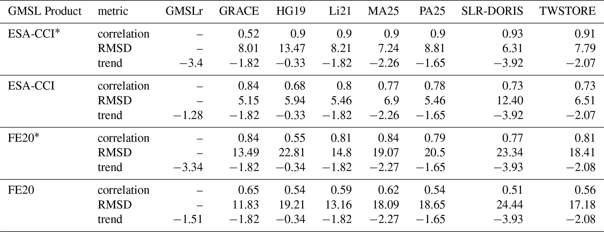
For the GRACE period 2003–2016 (Table 6), we find a similar picture, with a mismatch between the reconstructions and TWS+GL, as evidenced by the derived RMSD and trend values. However, RMSDs are considerably lower than when computed for the entire time period, ranging from 6.13 mm (TWSTORE) to 13.47 mm (HG19) for ESA-CCI and 14.8 mm (li21) to 22.81 mm (HG19) for FE20. Lower RMSDs indicate a good fit between reconstructions and LWS+GL in the early GRACE years, until about 2012, followed by a mismatch in the later years (Fig. 9), with the reconstruction underestimating the accelerated water loss after 2012. A higher agreement between LWS+GL and the reconstruction in the earlier GRACE years is expected, as nearly all reconstructions use a training period spanning 2003–2014. A similar behaviour is found for the correlations. The trend values for LWS and LWS+Gl are higher than for the entire time periods, indicating accelerated water mass loss in those years compared to those before 2003. The derived trends of the reconstructions, except for HG19, range between the trends derived from LWS, being −1.28 mm yr⁻¹ for ESA-CCI and −1.51 mm yr⁻¹ for FE20, and those for LWS+Gl, −3.4 and −3.34 mm yr⁻¹. The trend values derived here corroborate an accelerated loss of terrestrial water storage loss (Rodell et al., 2024; Chandanpurkar et al., 2025).

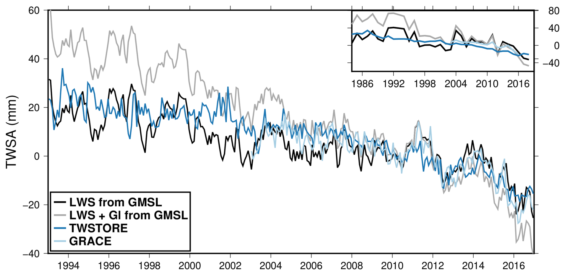
Figure 9 Time series of land water storage derived from the global mean sea level (GMSL), TWSTORE and GRACE. Main plot: GMSL Data from Horwath et al. (2021), the other data sets were deseasonalized; upper right inset: GMSL Data from Frederikse et al. (2020a), the other data sets were averaged to yearly means.

Table 5 Pearson correlation coefficient and RMSD of the reconstructions against GMSL derived land water storage, and trend of the data sets for 1993–2016 (GMSL product from Horwath et al., 2021) 1984–2018 (GMSL product from Frederikse et al., 2020a). The GMSL products were converted to land water heights. GMSLr (GMSL residual) denotes the GMSL-based TWSA. Rows marked with ^*: TWS = LWS+Glaciers; rows without: TWS = LWS. Trend: mm yr⁻¹ and RMSD: mm.

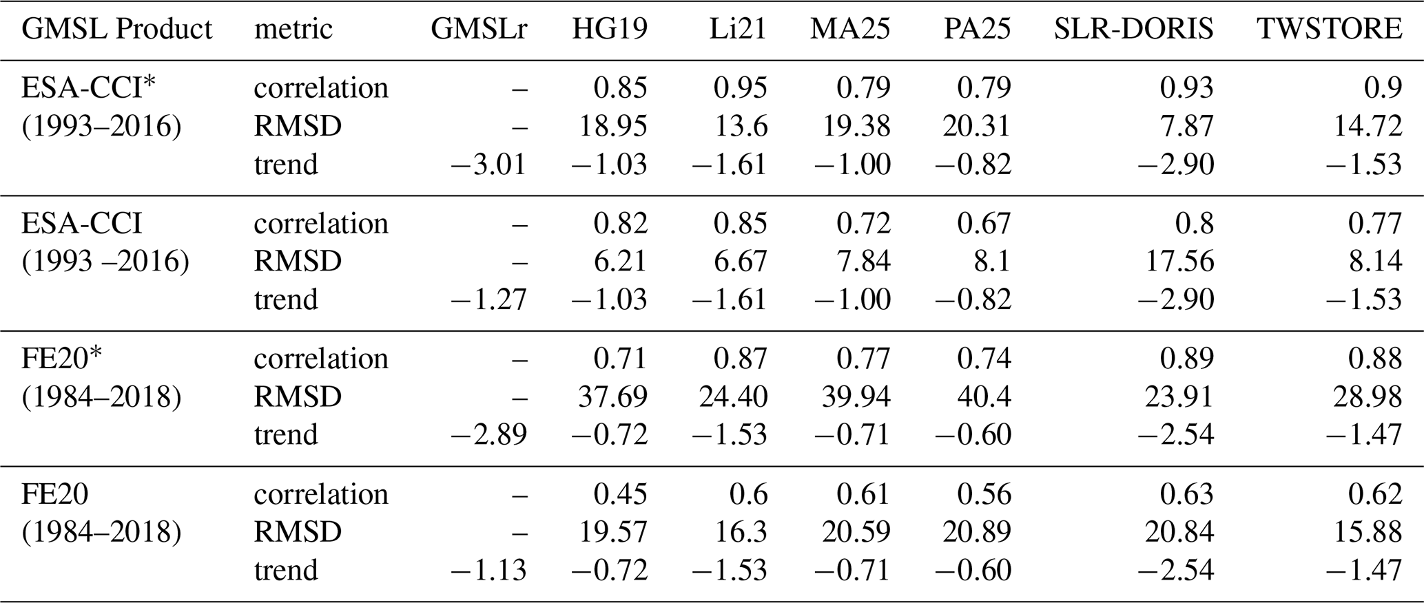
Table 6 Pearson correlation coefficient and RMSD of the reconstructions and GRACE against GMSL derived land water storage, and trend of the data sets for 2003–2016. The GMSL products were converted to land water heights GMSLr (GMSL residual) denotes the GMSL-based TWSA. Rows marked with ^*: TWS = LWS+Glaciers; rows without: TWS = LWS. Trend: mm yr⁻¹ and RMSD: mm. GRACE solution: ITSG-2018 (Table 1).

5.3 Terrestrial water budget and evapotranspiration

We used the reconstructed TWSA dataset in the continental water budget Eq. (15) to derive area-averaged time series of $\stackrel{\mathrm{‾}}{\mathrm{ET}}$ for 11 major river basins and compare them with GLEAM (Miralles et al., 2025) and ERA5 (Hersbach et al., 2020). The Pearson correlation coefficients (CC) of budget-derived $\stackrel{\mathrm{‾}}{\mathrm{ET}}$ with both GLEAM and ERA5 exceed values of $\mathrm{CC}\ge +\mathrm{0.60}$ for nine of the eleven assessed catchments (cf. Fig. 10), with median CCs of 0.73 (GLEAM) and 0.77 (ERA5). The strongest correlation (CC≥0.8) is observed for the Danube, Niger, Orange, and Mississippi river catchments. The weakest correlation by far (CC=0.1) is found for the Amazon basin, and for the upper Zambezi catchment (CC=0.5). Both areas represent dynamic regions of highest signal variations in TWSA (cf. Figs. C5 and C6). We use central differences in the budget approach to derive TWSA changes. The central differences are derived without temporal smoothing, making them prone to signal overamplification in noisy, dynamic environments, as the central differences operation emphasizes rapid changes. Signal overamplification in such dynamic environments can be lessened by employing a moderate low-pass filter. For the Amazon, using a ±3-month Gaussian smoother after computing the central differences raises the correlation with the reference ETs above 0.3 (0.2 and 0.4 for the 1984/2007 and 1997/2020 periods, respectively; not shown). Furthermore, budget results may be affected by phase/amplitude inconsistencies in the underlying data products or in the reference data. For example, when we substitute ERA5 “total precipitation” for GPCC in the budget approach, the (unfiltered) CC values for the Amazon increase by a factor of two (cf. the full correlation matrices in Fig. C8).

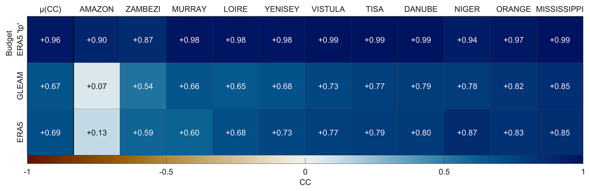
Figure 10 Catchment-wise Pearson correlation coefficient values of unfiltered budget-derived $\stackrel{\mathrm{‾}}{\mathrm{ET}}$ series 1984–2020 against ERA5, GLEAM, and a budget $\stackrel{\mathrm{‾}}{\mathrm{ET}}$ version where GPCC precipitation (in the budget equation) was replaced with ERA5 total precipitation. The table is horizontally sorted in ascending order by average correlation. The values of the first column (μ(CC)) represent the global mean CC of the 11 catchments, respectively.

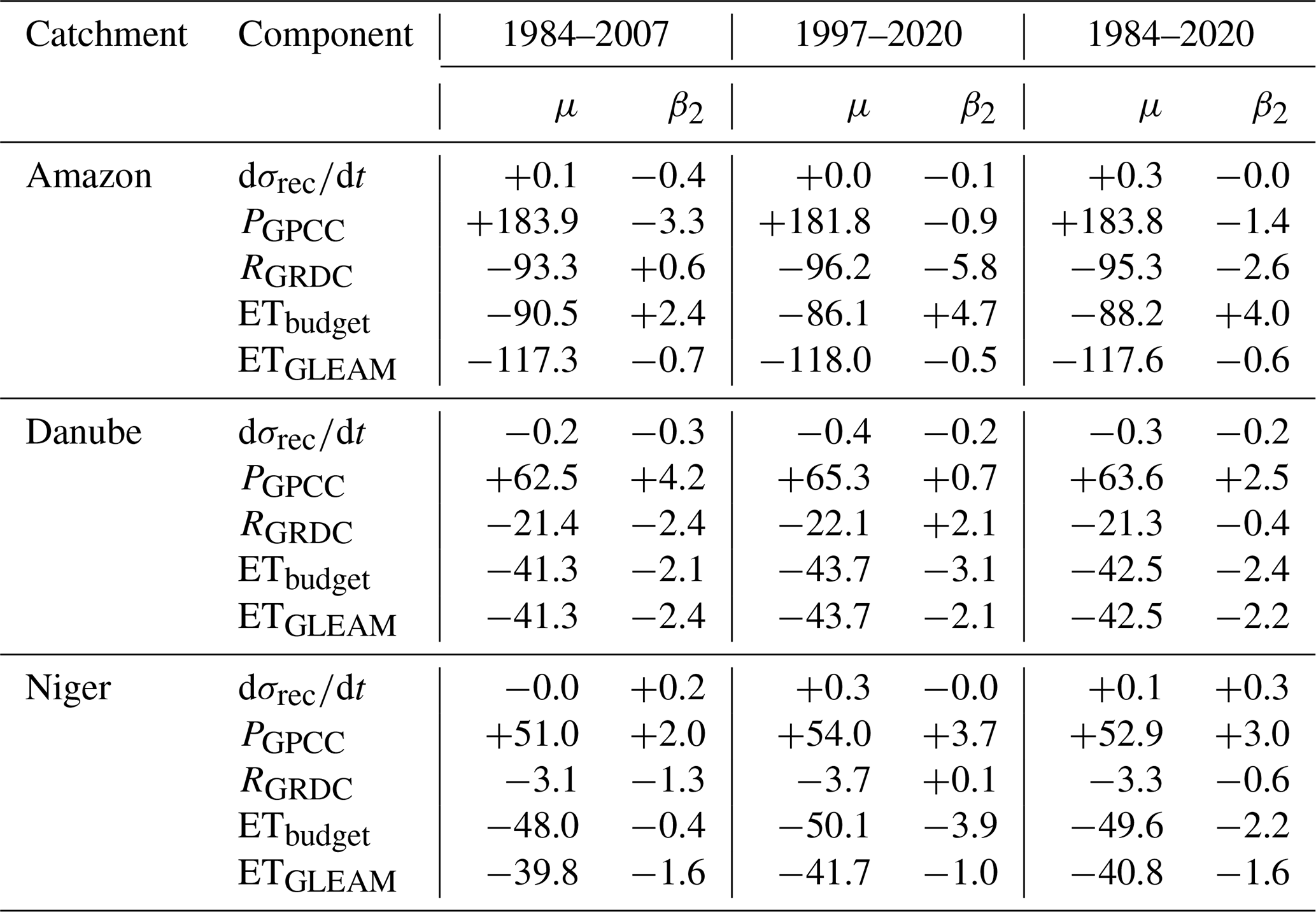
In the following, we highlight results for three representative regions, i.e., the river catchments defined by the Obidos (Amazon river), Ceatal (Danube river), and Niamey (Niger river) stations (Table B2 and Fig. C6). Results for eight additional catchments are provided in Table B1 in the Appendix. Table 7 summarizes the mean basin-averaged water mass fluxes over the entire reconstruction period and the two shorter periods as above, i.e., 1984 to 2007 and 1997 to 2020, derived from forming the budget. The derived $\stackrel{\mathrm{‾}}{\mathrm{ET}}$ time series are available at https://doi.org/10.5281/zenodo.16643628 (Gutknecht, 2025).

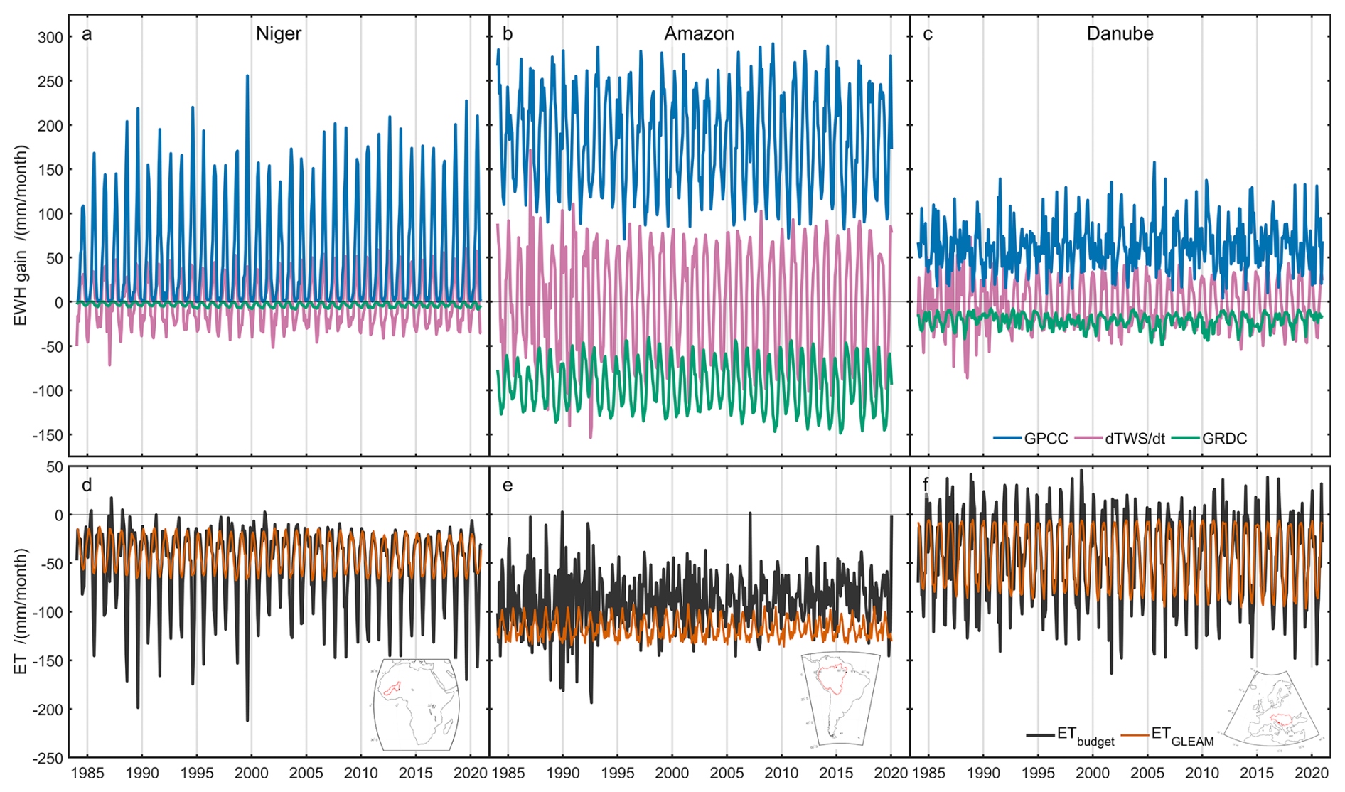
Figure 11 Terrestrial water budget monthly fluxes over the Niger, Amazon and Danube river catchments. The first row (a, b, c) shows in- and output expressed in equivalent water height (EWH) from (1) precipitation from GPCC (blue), (2) river discharge from GRDC (green), and (3) water storage change from reconstructed TWSA (purple). The second row (d, e, f) shows monthly $\stackrel{\mathrm{‾}}{\mathrm{ET}}$ (black) as derived using the budget equation with the upper row components, and “Actual Evaporation” from GLEAM (orange) for comparison, respectively. Positive fluxes represent net monthly water mass gain for the catchment and negative numbers represent net losses. For a version including ERA5 precipitation, see Fig. C7.

During all three assessed time frames, evapotranspiration rates for the Danube are found to be approximately 42 mm per month, which accounts for two-thirds of the total precipitation input. Terrestrial water storage net losses increased by 0.2 mm yr⁻² and annual precipitation intensified by 2.5 mm each year on average over 1984–2020. As monthly river discharge increased only by 0.7 mm between the two sub-periods, $\stackrel{\mathrm{‾}}{\mathrm{ET}}$ rates changed by 2.4 mm yr⁻² to account for increased P input and water storage losses. The mean of the budget-derived $\stackrel{\mathrm{‾}}{\mathrm{ET}}$ is in perfect agreement with GLEAM throughout the three assessed periods.

However, for the rather arid Niger upstream from Niamey, the net loss to the atmosphere estimated from the budget is 8.1 mm per month stronger than GLEAM suggests for the period 1984–2007 and 8.4 mm per month stronger for the period 1997–2020. The differences in evapotranspiration are mirrored in the precipitation differences recorded by GPCC and the ERA5 reanalysis, with GPCC depicting higher precipitation rates than ERA5, which can be attributed to more pronounced peaks in GPCC precipitation during summer months (Fig. 11a) and Figs. C7 and C9 in the Appendix. We observe the opposite behavior over the mostly tropical Amazon region, where the budget-derived $\stackrel{\mathrm{‾}}{\mathrm{ET}}$ is weaker by around 30 mm per month than seen in GLEAM. Furthermore, ERA5 mean monthly accumulated precipitation is 24 mm per month stronger than GPCC. However, observational and reanalysis products in the Niger and Amazon domains are hampered by low observation density. Our results suggest that in the Amazon basin, evapotranspiration rates have weakened by 4.4 mm between the two (overlapping) analysis periods. The decrease in evapotranspiration is only partially explained by decreases in P (2.1 mm) and increases in R (2.9 mm), while the water storage change remained relatively constant (decreased by less than 1 mm). We speculate that the lower evapotranspiration rate and the higher river discharge in the Amazon catchment could be related to the ongoing deforestation of the region (Coe et al., 2009). In the Niger basin, we observe an increase in P rates (+3.0 mm yr⁻²). The higher amount of P is compensated by 73 % by increasing $\stackrel{\mathrm{‾}}{\mathrm{ET}}$, by 19 % through more discharge, and by 8 % due to storage recharge.

It should be noted that opposite-sign $\stackrel{\mathrm{‾}}{\mathrm{ET}}$ fluxes (cf. Fig. 11f), i.e., from the atmosphere to the ground by means of condensation and deposition, can represent existing physical processes that are frequently observed during winter months in temperate and boreal climate zones. However, the amplitudes of the respective events in the budget-derived $\stackrel{\mathrm{‾}}{\mathrm{ET}}$ do not agree with those of GLEAM or ERA5 reanalysis. They may hint at unidentified offsets in some of the budget components. Here, as well, moderate low-pass filtering can reduce peak amplitudes to more realistic levels without significantly affecting inter-annual modes or decadal trends.

Table 7 Basin mean fluxes from evaluating the terrestrial water budget over the three periods. μ: temporal mean over monthly data; β₂: linear trend derived from a 6-parameter model. Mean fluxes are in units of mm per month, trends in mm yr⁻². Positive fluxes are defined as input into the integration domain, negative fluxes represent losses. Note that by this definition negative trends can also mean increased losses.

6 Data availability

The presented datasets are publicly available from: TWSTORE (https://doi.org/10.5281/zenodo.15827789, Hacker, 2025). Budget-derived ET time series (https://doi.org/10.5281/zenodo.16643628, Gutknecht, 2025). All datasets used in this article are available at the following locations: CSR mascon (https://www2.csr.utexas.edu/grace, last access: 6 August 2025, Rayner et al., 2003); GRACE L2 data: COST-G (https://doi.org/10.5880/COST-G.ICGEM_02_L2, Meyer et al., 2025), ITSG2018 (https://www.tugraz.at/institute/ifg/downloads/gravity-field-models/itsg-grace2018, Mayer-Gürr et al., 2018a); HadISST1 (https://www.metoffice.gov.uk/hadobs/hadisst/data/download.html, last access: 6 August 2025, Save, 2020), COBE-SST 2 (https://psl.noaa.gov/data/gridded/data.cobe2.html, last access: 6 August 2025, National Oceanic and Atmospheric Administration, Physical Sciences Laboratory, 2019), GPCC Version 2022 (https://doi.org/10.5676/DWD_GPCC/FD_M_V2022_050, Schneider et al., 2022), CPC global precipitation V1.0 (https://www.psl.noaa.gov/data/gridded/data.cpc.globalprecip.html, last access: 6 August 2025, National Oceanic and Atmospheric Administration, Physical Sciences Laboratory, 2016), CPC Soil Moisture v2 (https://www.psl.noaa.gov/data/gridded/data.cpcsoil.html, last access: 6 August 2025, National Oceanic and Atmospheric Administration, Physical Sciences Laboratory, 2017), GLEAM Soil Moisture v4.1a (https://www.gleam.eu/, last access: 6 August 2025, Miralles et al., 2025), GHCN CAMS Monthly Temperature (https://www.psl.noaa.gov/data/gridded/data.ghcncams.html, last access: 6 August 2025, National Oceanic and Atmospheric Administration, Physical Sciences Laboratory, 2025), Globmap LAI v3 (https://doi.org/10.5281/zenodo.4700264, Liu et al., 2021), Reconstruction by Li (2021): https://doi.org/10.5061/dryad.z612jm6bt, Reconstruction by Humphrey and Gudmundsson (2019a): https://doi.org/10.6084/m9.figshare.7670849, Reconstruction by Chandanpurkar et al. (2022a): https://doi.org/10.5281/zenodo.6659543; DORIS-SLR hybrid solution by Löcher et al. (2025a): https://doi.org/10.5880/ICGEM.2025.001; “ERA5 monthly data on single levels from 1940 to present” Total precipitation and Evaporation: https://doi.org/10.24381/cds.f17050d7 (Copernicus Climate Change Service, 2023); GLEAM Actual evaporation v4.2a (Miralles et al., 2025): sourced from sftp://hydras.ugent.be (last access: 10 February 2025) through https://www.gleam.eu (last access: 10 February 2025); GRDC streamflow: https://portal.grdc.bafg.de (Global Runoff Data Centre, 2025); HydroBASINS: https://www.hydrosheds.org (last access: 18 February 2026, Lehner et al., 2008).

7 Conclusions

We present a GRACE-like reconstruction of terrestrial water storage anomalies for the period 1984–2020, covering the entire global land area excluding Greenland and Antarctica. In contrast to earlier data sets, our reconstruction is derived as an optimal combination of a geodetic TWSA time series (derived from time-variable gravity data from the SLR and DORIS techniques) and a data-driven TWSA reconstruction based on climate data sets. The data-driven TWSA reconstruction is trained on the GRACE data from 2003 to 2010. Both TWSA data sets are transformed to a truncated basin-based EOF basis to remove and minimize noise in the input data, harmonized, and finally combined. The potential downside of the basin-wise approach is that correlations across basins are missed, and signal characteristics might change with the basin size. Since it is challenging to specify the uncertainty levels for the two TWSA data sets, we apply an iterative variance-component estimation procedure across their combination. The combined data also partially mitigate for the missing cross-correlations.
A comparison between the final reconstruction (TWSTORE), the preliminary reconstruction (i.e., before data combination), and the SLR-DORIS-only dataset revealed that the SLR-DORIS data influence the combination primarily on longer time scales. While the SLR-DORIS data add temporal reliability to our reconstruction, making it valuable for validation, they show a slight decrease in spatial resolution. A comparison with other independently derived reconstructions reveals a good agreement for long-term signals, except for the trend component. Our hypothesis is that inconsistencies across the trend estimates originate from the relatively short GRACE training period utilized for water storage reconstructions. This is related to the finding that GRACE trends should not be projected naively to the past.

A formal analysis of extreme values reveals that, over the last few decades, one-in-five-year storage deficits (surpluses) have reached 20–30 cm below (above) climatological conditions for some major river basins and up to 60 cm for one-in-ten-year deficits and surpluses. Using a sliding-window analysis, we find only minor temporal changes in these return levels, suggesting no intensification of water storage extremes. It is unclear whether extreme value theory provides a suitable framework for investigating hypotheses on water-cycle intensification and more frequent extremes. It is important to note that at the spatial and temporal scale of our reconstruction, extreme weather events, such as convective precipitation and the subsequent flooding, are not evident. The hydrological response to such events is probably more affected by river runoff and evapotranspiration than by changes in soil moisture storage, surface water levels, and groundwater recharge.

We compared GRACE-like TWSA reconstructions with LWS (GMSL- steric part- contribution from Greenland and Antarctica – inland glaciers) and LWS+Gl (GMSL – steric part – contribution from Greenland and Antarctica) from GMSL. We find a good agreement between the reconstructions and LWS from GMSL. The comparison with LWS+Gl showed a tendency for the reconstructions to underestimate water-mass loss from glacier melting. All datasets show a decline in TWSA, as reported by other studies. As a case study, we derive evapotranspiration rates from terrestrial water budgets using the presented reconstruction for a selection of globally distributed major river basins, based on observed river streamflow data. We found reduced evapotranspiration flux in the Amazon basin, which could only partly be attributed to reduced precipitation and increased runoff, suggesting a change in land cover. In the Niger basin, we find increased evapotranspiration rates that compensate for the increase in rainfall. The budget-derived $\stackrel{\mathrm{‾}}{\mathrm{ET}}$ correlates with GLEAM and ERA5 by CC≥0.6 in 82 % of the assessed basins. In regions with high (>5 cm) TWSA signal variation, we recommend the application of moderate temporal low-pass filtering if central-differencing (or comparable high-pass filters) is involved.

Our analysis demonstrates the potential of such long-term reconstructed data records to study changes in energy fluxes, water balance, and climate variables. We suggest that our extended observational TWSTORE record, although not directly observed, can be beneficial for analyzing terrestrial water budgets, despite its use of spatial constraints and higher noise in the earlier 1984–1992 period. The reconstruction also enables the evaluation of modeled water storage before the GRACE time frame at a spatial scale that does not conform to GRACE but is still valuable, for example, for validating CMIP runs.

Finally, we recognize that evaluating water storage reconstructions in the pre-GRACE era represents a challenging task, and we invite readers to propose new approaches for this purpose.

Appendix A: Methods

A1 Signal decomposition: Identifying dominant spatial and temporal patterns

Principal component analysis (PCA) is commonly used to reduce the dimensionality of a data set while preserving as much information as possible (Jolliffe, 2002). In general, GRACE L3 data are given on a 1° (≈ 110 km) or 0.5° grid (≈ 55 km). Reconstructing the GRACE time series for every grid point would be computationally expensive. Therefore, we reduce the dimensionality of the GRACE data using PCA, expressing the GRACE data into temporal (principal components (PCs) and spatial (empirical orthogonal functions (EOFs)) dominant modes. Assuming the spatial modes are constant over the reconstruction period, only the temporal modes are reconstructed.

Within the PCA, a new set of (transformed) uncorrelated variables, the principal components P_n x t (PCs),

$$\begin{array}{}\text{(A1)}& {\displaystyle }{\mathit{P}}_{n\text{x}t}={\mathit{X}}_{n\text{x}t}{\mathit{E}}_{n\text{x}n}\end{array}$$

are gained by projecting the data, X_n x t, with n being the spatial grid cells and t the epochs, onto a new orthogonal space, E_n x n, which represents the empirical orthogonal functions. The first m PCs contain most information, mostly 95 % of the total signal variance, whereas noise is mapped to the m+1…n PCs (Wold et al., 1987). The orthogonal space is gained from the eigenvectors of the empirical covariance matrix $\mathit{C}={\displaystyle \frac{\mathrm{1}}{t}}(\mathit{X}-\stackrel{\mathrm{‾}}{\mathit{x}}{)}^{\mathrm{T}}(\mathit{X}-\stackrel{\mathrm{‾}}{\mathit{x}})$ of the data. Using the m first modes, the data matrix can be restored by

$$\begin{array}{}\text{(A2)}& {\displaystyle }{\stackrel{\mathrm{‾}}{\mathit{X}}}_{n\text{x}t}={\stackrel{\mathrm{‾}}{\mathit{E}}}_{n\text{x}m}{\stackrel{\mathrm{‾}}{\mathit{P}}}_{m\text{x}t}\end{array}$$

We apply the PCA to the GRACE data splitting it into PCs and EOFs. The predictors and the SLR-DORIS data are then projected onto the GRACE derived EOF basis as

$$\begin{array}{}\text{(A3)}& {\displaystyle }\mathit{P}{\mathit{C}}_{n\text{x}t}={\mathit{D}}_{n\text{x}t}{\mathit{E}}_{n\text{x}n}\end{array}$$

with PC denoting the projected data and D the specific data set.

A2 Variance component estimation

Variance component estimation (VCE) is a weighting technique for observations in the context of least-squares adjustment. A well-known example of the application of VCE is the combination of gravity data in the context of gravity field modeling or geopotential determination (Koch and Kusche, 2002; Brockmann and Schuh, 2010; Fecher et al., 2015).

Given a linear normal equation system in terms of a least squares adjustment (linearized Gauss- Markoff Model (Koch, 2004))

$$\begin{array}{}\text{(A4)}& {\displaystyle }\mathit{l}+\mathit{v}=\mathit{A}\mathit{x}\mathbf{\Sigma }\mathit{\left\{}\mathcal{L}\mathit{\right\}}={\mathit{\sigma }}_{\mathrm{0}}^{\mathrm{2}}{\mathit{Q}}_{ll}\end{array}$$

x describes the parameters of the adjustment. The matrix A, also called design matrix, maps the observation to the parameter space, v are the residuals, and Σ{𝓛} the covariance matrix of the observations. The variance component ${\mathit{\sigma }}_{\mathrm{0}}^{\mathrm{2}}$ scales the co-factor matrix Q_ll and is a mostly unknown random variable. The least squares solution for the unknown parameters x reads

$$\begin{array}{}\text{(A5)}& {\displaystyle }\widehat{\mathit{x}}{\displaystyle }={\mathit{N}}^{-\mathrm{1}}\mathit{n}\end{array}$$

with $\mathit{N}={\mathit{A}}^{\mathrm{T}}({\mathit{\sigma }}_k^{\mathrm{2}}{\mathit{Q}}_{l_k{l}_k}{)}^{-\mathrm{1}}\mathit{A}$ being the normal equation matrix and $\mathit{n}={\mathit{A}}^{\mathrm{T}}({\mathit{\sigma }}_k^{\mathrm{2}}{\mathit{Q}}_{l_k{l}_k}{)}^{-\mathrm{1}}\mathit{l}$ the normal equation vector. If A has full rank, solving the above system of equations leads to the optimal solution in the least squares sense.

Assuming l is composed of n independent groups, we can sequentially sum up the normal equations for each observation group, leading to

$$\begin{array}{}\text{(A6)}& {\displaystyle }\sum _{k=\mathrm{1}}^n{\mathit{\sigma }}_k^{\mathrm{2}}{\mathit{N}}_k\mathit{x}=\sum _{k=\mathrm{1}}^n{\mathit{\sigma }}_k^{\mathrm{2}}{\mathit{n}}_k\end{array}$$

The unknown variance components ${\mathit{\sigma }}_k^{\mathrm{2}}$ are estimated iteratively from the residuals, catching as many uncertainties from the data as possible (Förstner, 1979). Based on the maximum-likelihood method or the best invariant quadratic unbiased estimation (Koch, 2018; Förstner, 1979), the estimated variance components are given as

$$\begin{array}{}\text{(A7)}& \begin{array}{rl}{\mathit{\sigma }}_k^{{\mathrm{2}}^{\left(p\right)}}& ={\displaystyle \frac{{\mathit{v}}_k^{\mathrm{T}}({\mathit{\sigma }}_k^{{\mathrm{2}}^{(p-\mathrm{1})}}{\mathit{Q}}_{l_k{l}_k}{)}^{-\mathrm{1}}{\mathit{v}}_k}{r_k}}\text{with}{\mathit{v}}_k={\mathit{A}}_k{\widehat{\mathit{x}}}_k-{\mathit{l}}_k\\ & \text{and}{r}_k=u_k-\mathrm{tr}\left({\mathit{N}}_k{\mathit{N}}^{-\mathrm{1}}\right)\end{array}\end{array}$$

with p referring to the iteration step, r_k is the redundancy and u_k the number of observations of the individual observation group k.

We use VCE for the data combination not on the normal equation level but on the observational level, stating that the parameters x are directly observed, leading to A_k being the identity matrix.

A3 Granger causality

Granger causality (Granger, 1969), is a statistical method to determine temporal, predictive causality between two or more time series. Given two time series $\mathit{l}=[l_{\mathrm{1}},l_{\mathrm{2}},\mathrm{\dots },l_n]$ and $\mathit{y}=[y_{\mathrm{1}},y_{\mathrm{2}},\mathrm{\dots },y_n]$ with n being the length of the time series, y Granger causes l if incorporating y in the forecast of l improves the forecast of l.

Under the assumption of stationarity (marginal distribution does not change over time/space), causal sufficiency (all influencing variables are observed) and linear dependencies between the time series Granger (1969) employed an autoregressive (AR) process of order p to describe the relationship between the time series, leading to the two predictive models.

$$\begin{array}{ll}{\displaystyle }\widehat{l_t}& {\displaystyle }={\mathit{\beta }}_{\mathrm{01}}+\sum _{p=\mathrm{1}}^p\left({\mathit{\beta }}_{\mathrm{11}p}l(t-p)+{\mathit{\beta }}_{\mathrm{12}p}y(t-p)\right)+\mathit{ϵ}\\ \text{(A8)}& {\displaystyle }& {\displaystyle }\text{full model}\text{(A9)}& {\displaystyle }\widehat{l_t}& {\displaystyle }={\mathit{\beta }}_{\mathrm{01}}+\sum _{p=\mathrm{1}}^p\left({\mathit{\beta }}_{\mathrm{11}p}l(t-p)\right)+\mathit{ϵ}\text{baseline model}\end{array}$$

y Granger causes l if at least one of the parameters β_12p is non zero, leading to the null hypothesis (e.g Attanasio (2012))

$$\begin{array}{}\text{(A10)}& {\displaystyle }{H}_{\mathrm{0}}:{\mathit{\beta }}_{\mathrm{121}}={\mathit{\beta }}_{\mathrm{122}}=\mathrm{\dots }={\mathit{\beta }}_{\mathrm{12}p}=\mathrm{0}\text{non causality}\end{array}$$

A F-test is typically used to determine, whether incorporating y leads to an improvement in the prediction of l. The F-test assumes that the residuals are Gaussian distribution. However, earth-related observations are not normal distributed. Papagiannopoulou et al. (2017).

Instead of a F-test we follow Papagiannopoulou et al. (2017) and employ the coefficient of determination

$$\begin{array}{}\text{(A11)}& {\displaystyle }{R}^{\mathrm{2}}=\mathrm{1}-{\displaystyle \frac{{\sum }_{i=p+\mathrm{1}}^N(l_i-\widehat{l_i}{)}^{\mathrm{2}}}{{\sum }_{i=p+\mathrm{1}}^N(l_i-\stackrel{\mathrm{‾}}{l}{)}^{\mathrm{2}}}}\end{array}$$

with $\widehat{l_i}$ being the forecast of l_i and $\stackrel{\mathrm{‾}}{l}$ the mean of l_i. In the literature, R² is also known as the Nash–Sutcliffe model efficiency coefficient, a common metric in hydrology and climate science. R² can also be interpreted as the forecasting model's fraction of the explained variance. The optimal value for R² is 1, which corresponds to an error-free forecast ($\widehat{l_i}=l_i$). Values R²<0 indicate that the forecast error is larger than the observed error and R²=0 indicates that the model has the same predictive skill as the mean of the observed time series. If $R^{\mathrm{2}}(\mathit{l},\widehat{\mathit{l}})$ increases when $y(t-\mathrm{1}),y_{(}t-\mathrm{2}),\mathrm{\dots },y(t-n)$ is included in the prediction of l, then y Granger causes l.

A4 Generalized extreme value (GEV) distribution

Extreme value theory provides the statistical framework for estimating the probability of singular or extreme events. Generalized extreme value (GEV) distribution functions are a family of continuous probability distributions within the extreme value theory. Three parameters describe the GEV: shape ξ (tail behavior of the distribution), location μ (location or shift of the distribution), and scale σ (spread of the distribution). The GEV is built upon the three subfamilies: The Gumbel (ξ=0), the Fréchet (ξ>0), and the Weibull (ξ<0) distributions, leading to the cumulative distribution function

$$\begin{array}{}\text{(A12)}& {\displaystyle }F\left(z\right)=\left\{\begin{array}{ll}\exp (-(\mathrm{1}+\mathit{\xi }{\displaystyle \frac{z-\mathit{\mu }}{\mathit{\sigma }}}{)}^{-\mathrm{1}/\mathit{\xi }})& \mathit{\xi }\ne \mathrm{0}\\ \exp \left(\exp \right(-{\displaystyle \frac{z-\mathit{\mu }}{\mathit{\sigma }}}\left)\right)& \mathit{\xi }=\mathrm{0}\end{array}\right.\end{array}$$

The quantiles z_p at probability p can be derived as

$$\begin{array}{}\text{(A13)}& {\displaystyle }{z}_p=\left\{\begin{array}{ll}\mathit{\mu }-\mathit{\sigma }/\mathit{\xi }(\mathrm{1}-(-\text{log}(\mathrm{1}-p){)}^{-\mathit{\xi }}& \mathit{\xi }\ne \mathrm{0}\\ \mathit{\mu }-\mathit{\sigma }\text{log}\left(\right(-\text{log}(\mathrm{1}-p))& \mathit{\xi }=\mathrm{0}\end{array}\right.\end{array}$$

We interpret z_p as the return level interval for probability p, which means that an expected extreme occurs after p years.

We follow the approach of Kusche et al. (2016), which is based on Martins and Stedinger (2000) to derive the parameters of the GEV.

To estimate the GEV distribution, we first reduced a six-parameter model and the climatology from the grid time series. We then select the annual maximum and minimum anomalous storage values. Using this shortened time series, we estimate the GEV parameters through Moment Estimation (ME) (Martins and Stedinger, 2000). The GEV parameters are calculated based on the first moment (mean), the second moment (standard deviation), and the third moment (skewness) of the time series, leading to

$$\begin{array}{}\text{(A14)}& \begin{array}{rl}\widehat{x}& ={\displaystyle \frac{\mathrm{1}}{n}}\sum _{j=\mathrm{1}}^n{x}_j,\widehat{s}=\left({\displaystyle \frac{\mathrm{1}}{n}}\sum _{j=\mathrm{1}}^n\right(x_j-\widehat{x}{)}^{\mathrm{2}}{)}^{\mathrm{1}/\mathrm{2}},\\ & \widehat{g}={\displaystyle \frac{\mathrm{1}}{n}}\sum _{j=\mathrm{1}}^n{\displaystyle \frac{(x_j-\widehat{x}{)}^{\mathrm{3}}}{\widehat{s^{\mathrm{3}}}}}\end{array}\end{array}$$

With x denoting the time series and n the number of observations. From the skewness, the shape parameter is iteratively solved via

$$\begin{array}{}\text{(A15)}& {\displaystyle }\text{sign}\left(\widehat{\mathit{\xi }}\right){\displaystyle \frac{-{\mathrm{\Gamma }}_{\mathrm{3}}\left(\widehat{\mathit{\xi }}\right)+\mathrm{3}{\mathrm{\Gamma }}_{\mathrm{1}}\left(\widehat{\mathit{\xi }}\right){\mathrm{\Gamma }}_{\mathrm{2}}\left(\widehat{\mathit{\xi }}\right)-\mathrm{2}{\mathrm{\Gamma }}_{\mathrm{1}}^{\mathrm{3}}\left(\widehat{\mathit{\xi }}\right)}{\left({\mathrm{\Gamma }}_{\mathrm{2}}\right(\widehat{\mathit{\xi }})-{\mathrm{\Gamma }}_{\mathrm{1}}^{\mathrm{2}}(\widehat{\mathit{\xi }}){)}^{\mathrm{3}/\mathrm{2}}}}=\widehat{g}\end{array}$$

where ${\mathrm{\Gamma }}_n\left(\widehat{\mathit{\xi }}\right)=\mathrm{\Gamma }(\mathrm{1}+n\widehat{\mathit{\xi }})$ and Γ() is the Gamma function. The location and shape parameter is then derived as

$$\begin{array}{}\text{(A16)}& \widehat{\mathit{\sigma }}={\displaystyle \frac{\widehat{s}\left|\widehat{\mathit{\xi }}\right|}{\left({\mathrm{\Gamma }}_{\mathrm{2}}\right(\widehat{\mathit{\xi }})-{\mathrm{\Gamma }}_{\mathrm{1}}^{\mathrm{2}}(\widehat{\mathit{\xi }}){)}^{\mathrm{1}/\mathrm{2}}}},\widehat{\mathit{\mu }}=\widehat{x}-{\displaystyle \frac{\widehat{\mathit{\sigma }}}{\widehat{\mathit{\xi }}}}(\mathrm{1}-{\mathrm{\Gamma }}_{\mathrm{1}}(\widehat{\mathit{\xi }}\left)\right)\end{array}$$

Appendix B: Terrestrial water budget and evapotranspiration

In addition to the three river catchments presented in the main article, we derived $\stackrel{\mathrm{‾}}{\mathrm{ET}}$ using the terrestrial water budget equation for a wider selection of basins. Table B1 summarizes the fluxes of the budget components, respectively. Table B2 gives an overview of the exact stations and corresponding HydroSHED-based shapes used for the budget analysis. For the location of the analyzed catchments and the corresponding gauge stations, see Fig. C6.

Table B1 Basin-averaged fluxes from evaluating the terrestrial water budget over the three periods. μ: temporal mean over monthly data; β₂: linear trend derived from a 6-parameter model. Mean fluxes are given in millimetre per month, trends in millimetres per year squared. Positive fluxes are defined as input into the integration domain, negative fluxes represent losses. Note that by this definition negative trends can also mean increased losses.

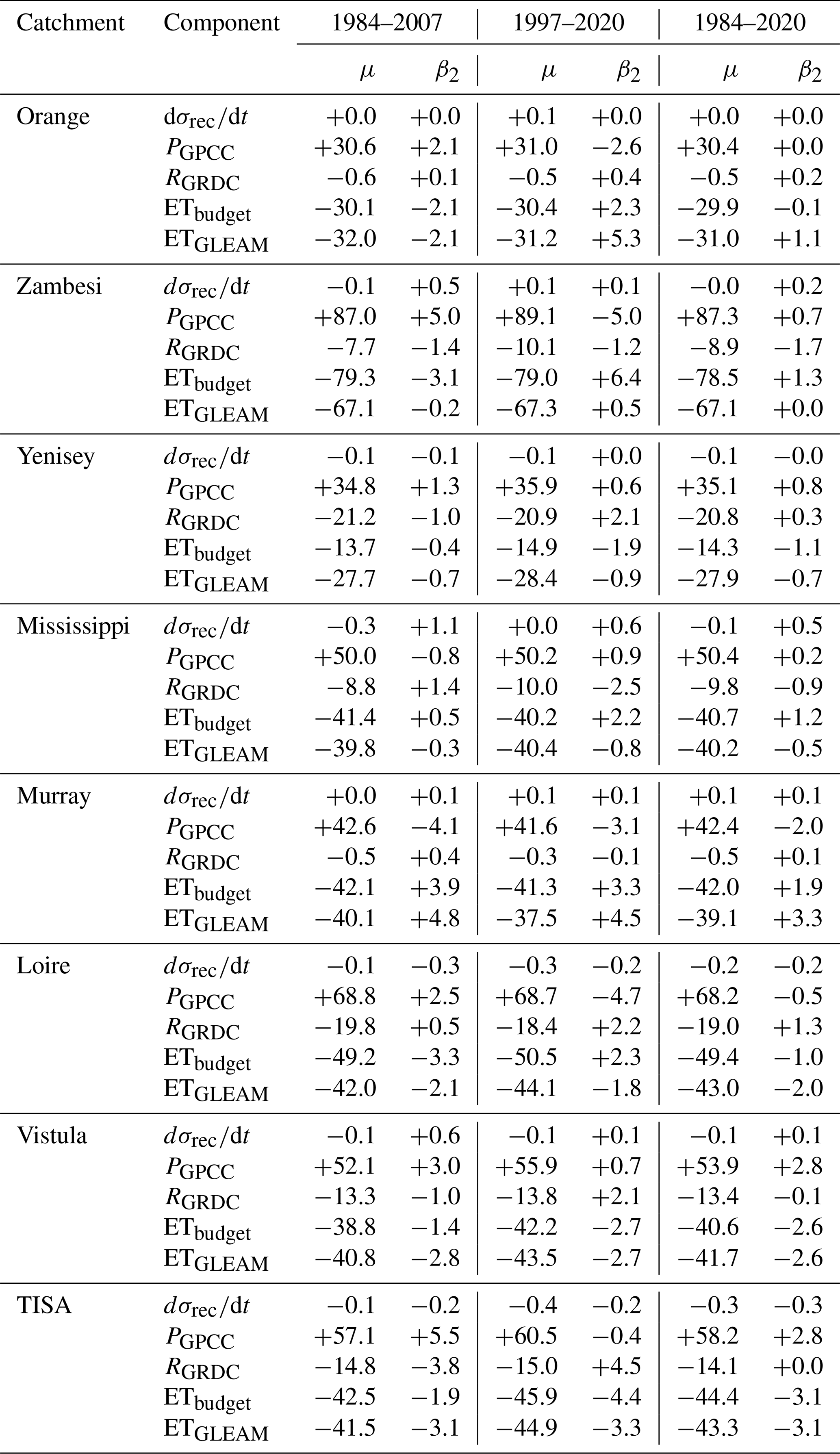
Table B2 Detailed list of GRDC stations and corresponding shape area used in the budget analysis. Last column is the number of months with discharge observations available over the targeted 1984–2020 time frame (i.e. N=444). ^a Missing month in June 1994; ^b missing month in October 2019; ^c no data after December 2017; ^d no data after January 2020; ^e missing months in April and May 2017.

Appendix C: Additional plots

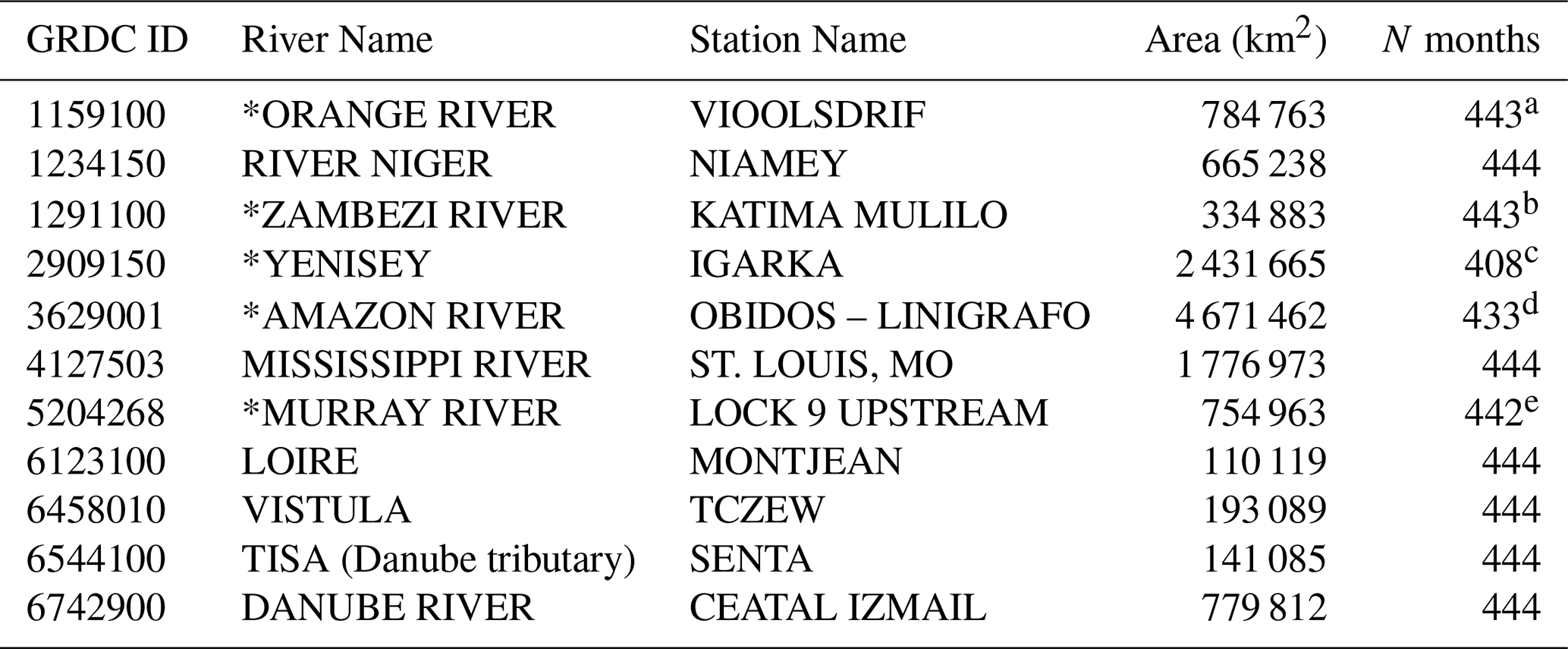
The reconstruction is performed on a polygon scale. For every polygon, the reconstruction procedure is applied. The number of dominant modes selected in the PCA differs depending on the polygon's size and location. Figure C1 illustrates the number of dominant modes per polygon such that 95 % of the signal properties are covered. For the data combination, the polygons used for the reconstruction are aggregated to “bigger” polygons to account for the lower spatial resolution of the SLR data (Fig. C2). The number of modes selected for the aggregated polygons is shown in Fig. C3. We also provide uncertainty information for our reconstructions. The information is given as variances only. Figure C5 displays the temporally averaged standard deviation for TWSTORE. The selected catchments for the budget analysis are depicted in Fig. C6. For a comparison of the impact on budget-derived $\stackrel{\mathrm{‾}}{\mathrm{ET}}$ of using ERA5 precipitation instead of GPCC, see Figs. C7 and C9. In the Niger catchment, the stronger peak precipitation in GPCC during summer causes higher $\stackrel{\mathrm{‾}}{\mathrm{ET}}$. And in the Amazon catchment, the relatively “wetter” ERA5 precipitation leads to stronger $\stackrel{\mathrm{‾}}{\mathrm{ET}}$ fluxes compared to GPCC.

C1 Number of modes per polygon

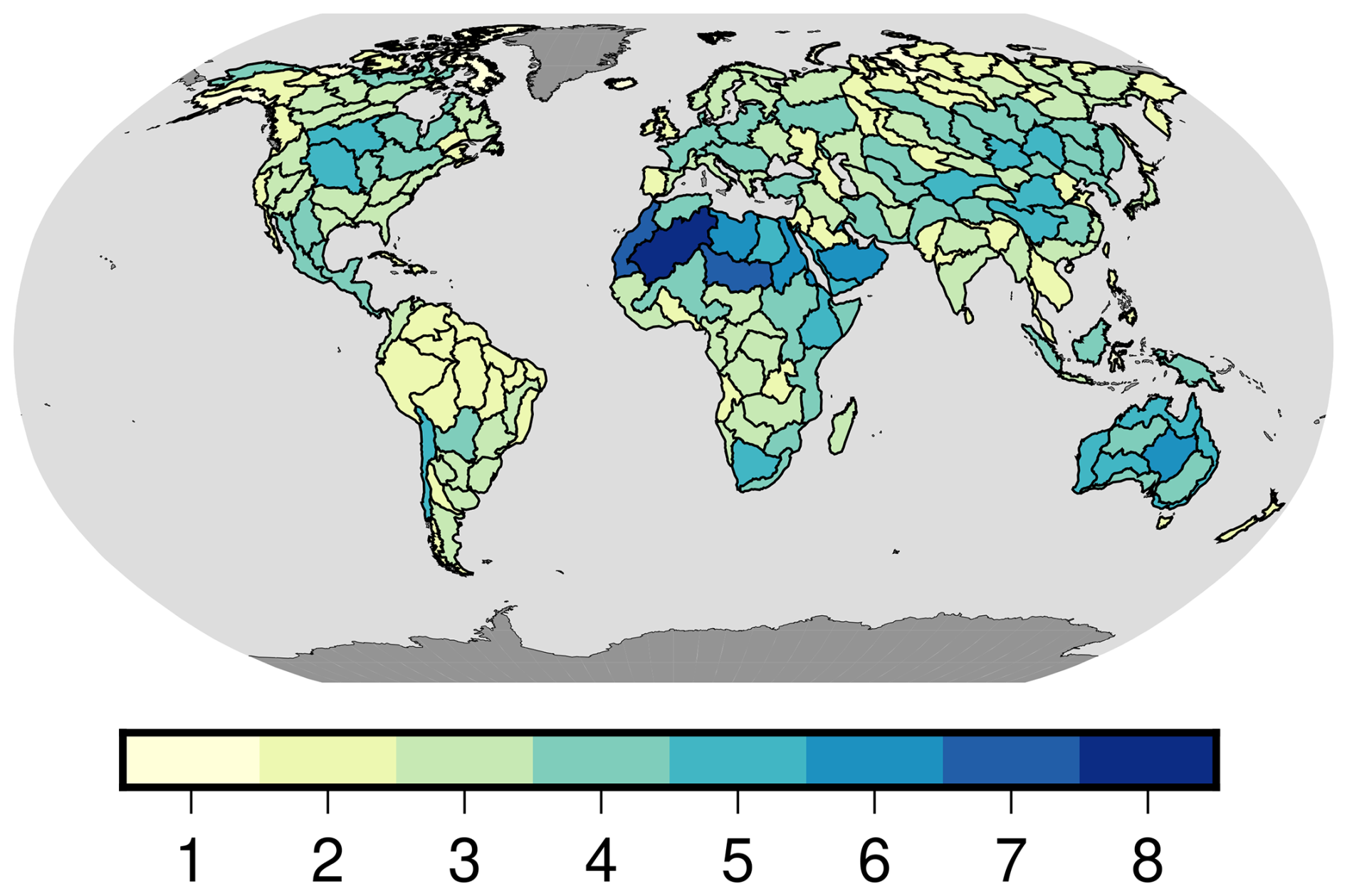
Figure C1 Number of modes per polygon used for the reconstruction. The number of polygons is 222.

C2 Polygons used for the data combination

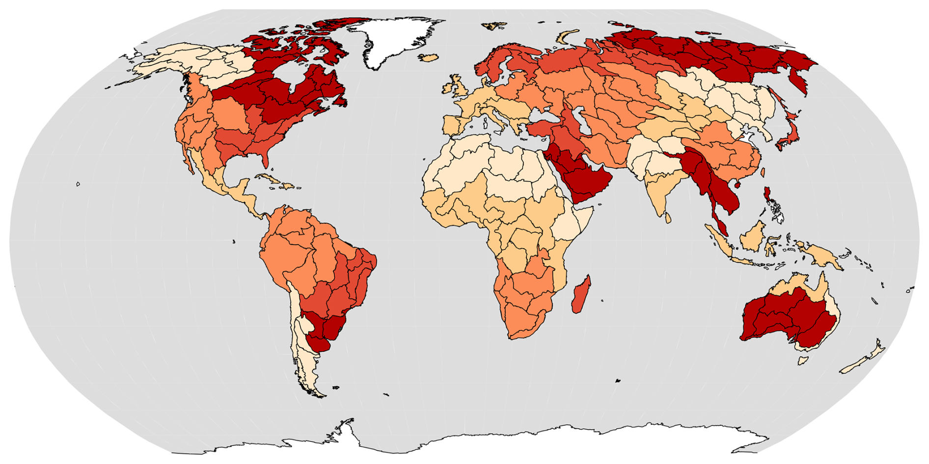
Figure C2 Overview of the polygons used for the data combination. Polygons of the same color and spatial orientation are grouped together.

C3 Number of dominant modes per polygon for the data combination

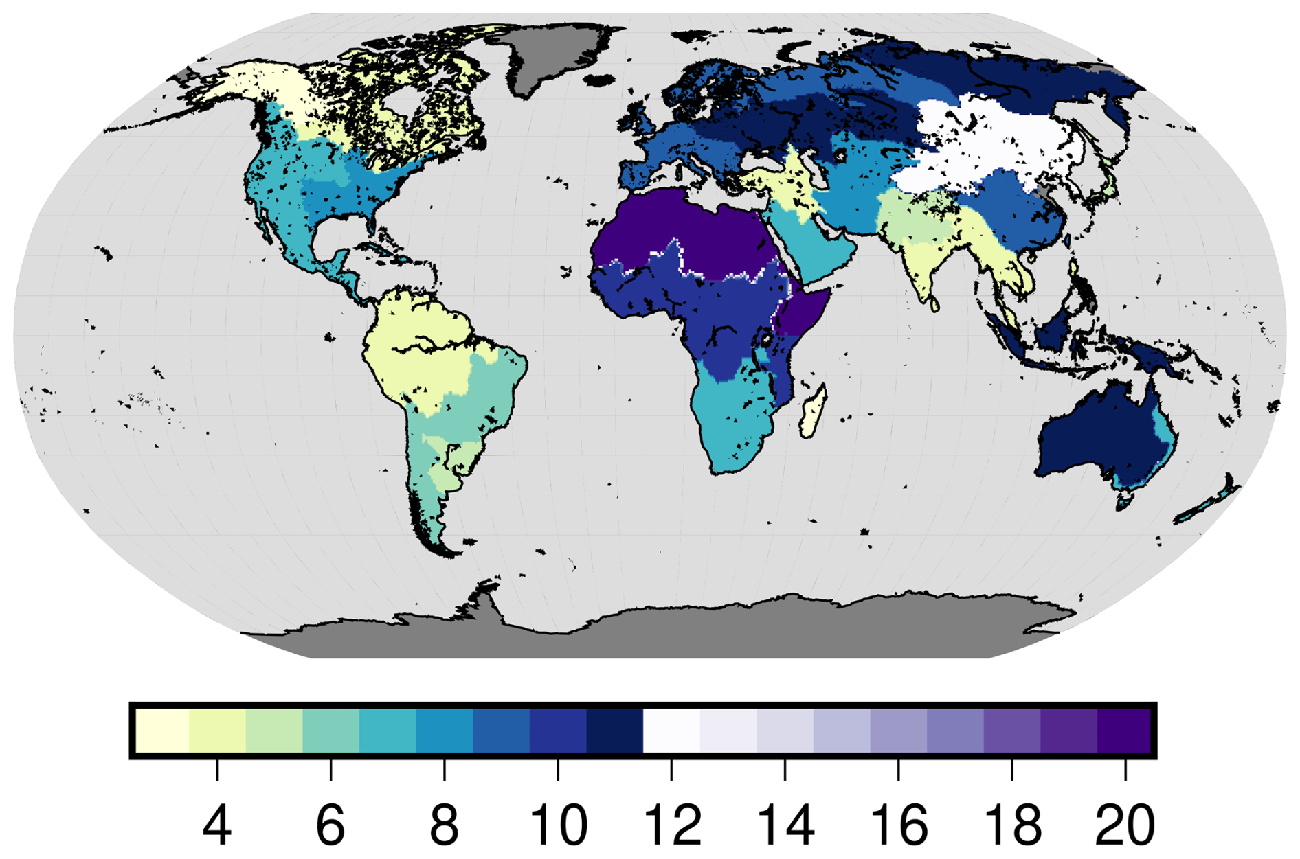
Figure C3 Number of modes per polygon used for the data combination.

C4 Regions for the computation of the area-averaged time series

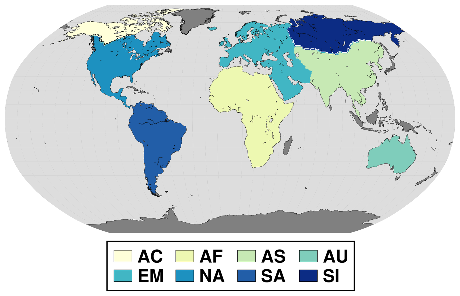
Figure C4 (Sub) continents as defined by the HydroBasins (Lehner and Grill, 2013) from Hydrosheds. AC: Arctic northern Canada, AF: Africa, AS: Asia, AU: Australia; EM: Europe and Middle East, NA: (central) Northern America, SA: South America, SI: Siberia.

C5 Variances of TWSTORE

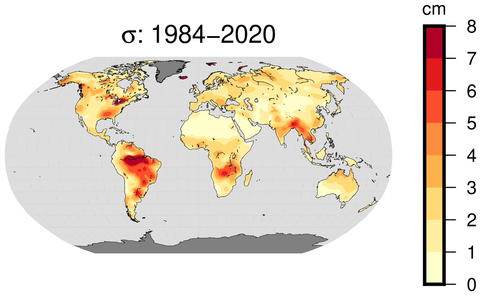
Figure C5 Averaged standard deviation of TWSTORE over 1984 to 2020. High standard deviations correspond to regions with high TWSA signal variations.

C6 Location of river catchments used in the budget analysis

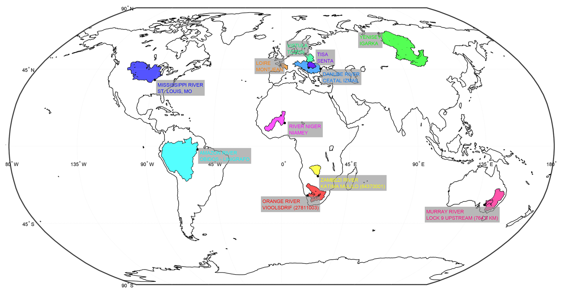
Figure C6 World map with locations of catchments analyzed for water budgets.

C7 ET_budget time series in comparison with ERA5

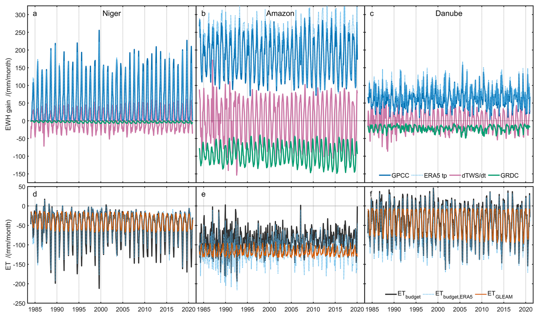
Figure C7 Terrestrial water budget monthly fluxes over the Niger, Amazon and Danube river catchments. The first row (a, b, c) shows in- and output expressed in equivalent water height from (1) precipitation from GPCC (solid blue), (2) river discharge from GRDC (green), and (3) water storage change from reconstructed TWSA (purple). The second row (d, e, f) shows monthly $\stackrel{\mathrm{‾}}{\mathrm{ET}}$ (black) as derived using the budget equation with the upper row components, and “Actual Evaporation” from GLEAM (orange) for comparison, respectively. Positive fluxes represent net monthly water mass gain for the catchment and negative numbers represent net losses. The dotted blue curves in (a)–(c) shows precipitation from ERA5 reanalysis for comparison. And the dotted blue curves in (d)–(f) depict budget-derived $\stackrel{\mathrm{‾}}{\mathrm{ET}}$ when ERA5 total precipitation instead of GPCC is used.

C8 Pearson CCs of ET time series

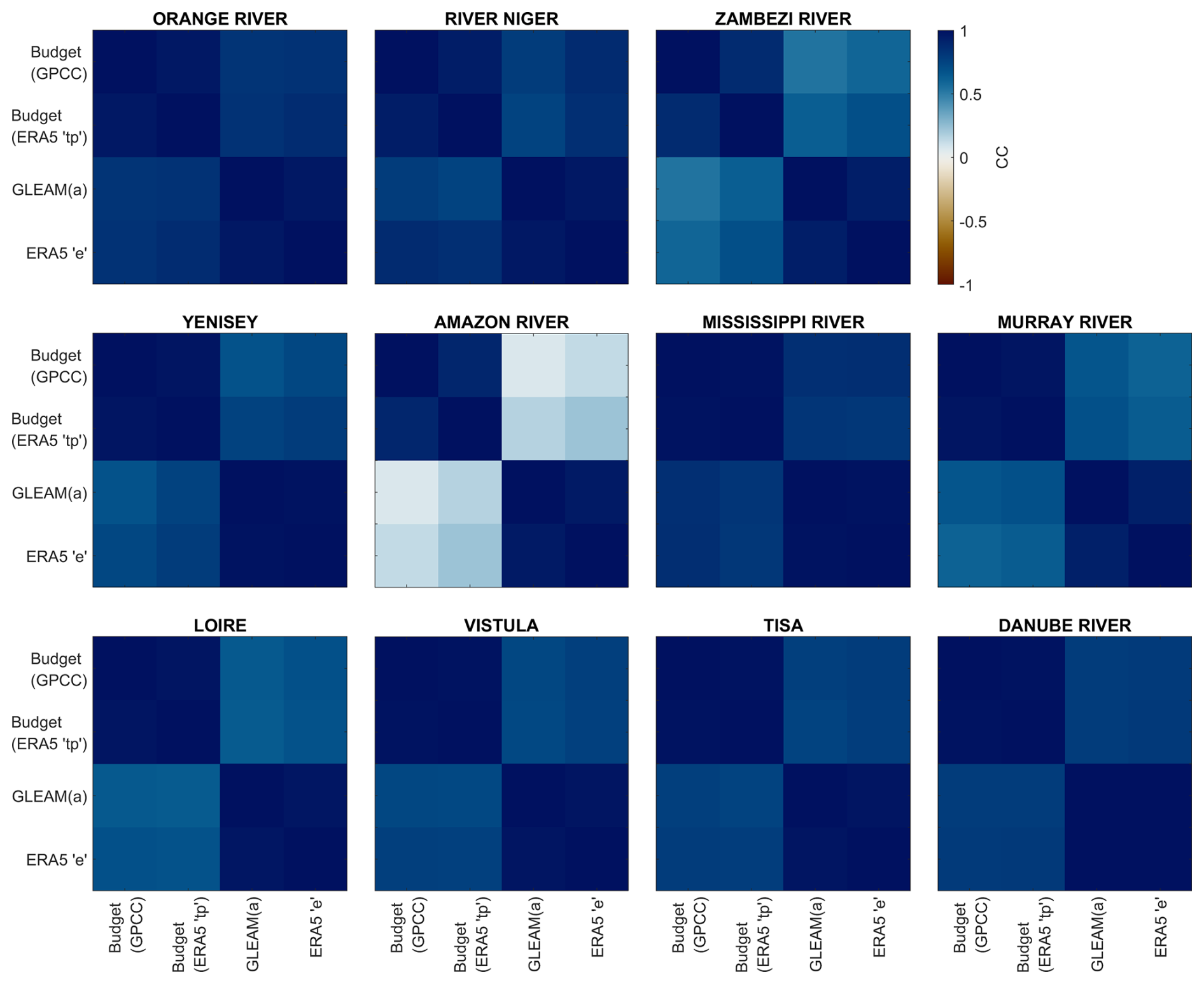
Figure C8 Catchment-wise Pearson correlation coefficient values of $\stackrel{\mathrm{‾}}{\mathrm{ET}}$ time series 1984–2020. Here, in addition to Fig. 10, all the combinations of budget-derived $\stackrel{\mathrm{‾}}{\mathrm{ET}}$ (with GPCC precipitation), ERA5 (“e”), GLEAM, and a budget $\stackrel{\mathrm{‾}}{\mathrm{ET}}$ version where GPCC precipitation (in the budget equation) was replaced with ERA5 total precipitation (“tp”) are shown.

C9 GPCC and ERA5 precipitation comparison

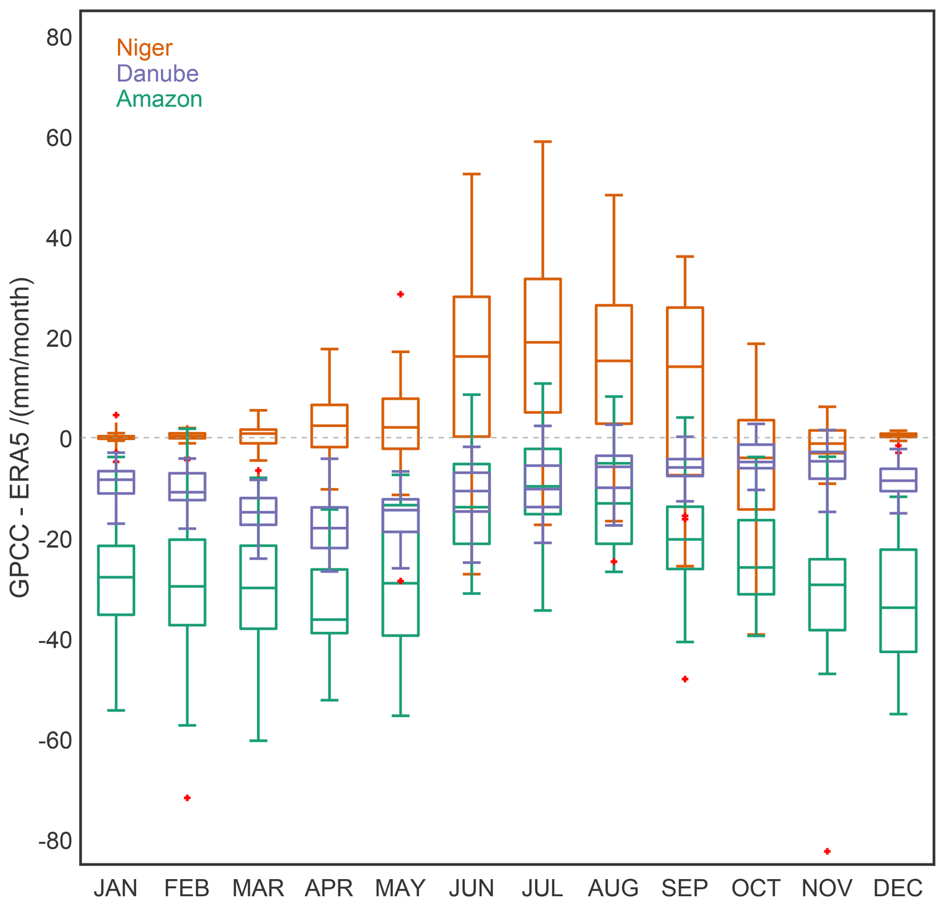
Figure C9 Monthly climatological comparison of GPCC and ERA5 precipitation over the Niger-, Amazon- and Danube-catchments, derived from the monthly aggregated area-averaged precipitation time series for GPCC minus those for ERA5. Note how the (relative) ERA5 wet bias in the Amazon region can explain the offset in the budget-derived $\stackrel{\mathrm{‾}}{\mathrm{ET}}$, whereas the ERA5 dry-bias during peak-precipitation months in the summer in the Niger catchment leads to less pronounced budget-derived $\stackrel{\mathrm{‾}}{\mathrm{ET}}$. On each box, the central mark indicates the median, and bottom and top edges indicate the 25th to 75th percentile, respectively. Thin vertical lines represent the spread range, excluding outliers (red crosses).