A comprehensive global mapping of offshore lighting

We present the first comprehensive multiyear global mapping of offshore lighting structures derived from low-light imaging satellite observations collected at night. The sensor is the day–night band (DNB) flown as part of the NASA/NOAA Visible Infrared Imaging Radiometer Suite (VIIRS). The product merges two operational nighttime light products: VIIRS boat detection (VBD) data and VIIRS cloud-free nighttime light (VNL) data. The two products are spatially complementary, making it possible to fill gaps through a merger. Both product sets have an average DNB radiance layer, and the merger involves preserving the higher of the two average radiances. A wide range of lighting structures is present, i.e., fishing grounds, platforms, anchorages, gas flares, transit routes, and the glow surrounding bright lighting onshore. The richness of the numbers and types of offshore lighting structures can be traced back to the DNB spike detector at the core of the VBD algorithm. The VNL algorithm uses outlier removal to filter out biomass burning, an essential process for mapping electric lighting onshore. The outlier removal drops about 80 % of the offshore lighting detections. We expect that the new product will lead to an improved understanding of fishing grounds, offshore light pollution, and supply chain disruptions at anchorages, thereby aiding in the development of more sustainable and efficient practices. The global datasets are available at https://doi.org/10.25676/11124/179157 (Elvidge et al., 2024).

1 Introduction

In 2015–2016 I heard a frequent question from users of the satellite boat detection data my team produced and distributed. The algorithm reports the location and brightness of offshore lights at night from NASA/NOAA Visible Infrared Imaging Spectrometer Suite (VIIRS) day–night band (DNB) data in near real time (Elvidge et al., 2015a). The initial VIIRS boat detection (VBD) production area was Indonesia and the Philippines, under contract with the U.S. Agency for International Development. We provided near-real-time VBD data, technical support, and training to the two governments. They used VBD data to monitor fishery closures, marine protected areas, and fishing grounds. Both governments continue to use the VBD data to this day.

The most common question from the users was how they could distinguish between boats using lights for fishing and other offshore lighting. My response was that “If a VBD pixel is in a fishing ground – it is likely fishing.” It turned out that Indonesia and the Philippines divide their waters up into regional sections, and neither had a specific “fishing-ground map.” With no existing map, we decided to make our own with temporal compositing of VBD data. The temporal compositing worked – making it possible to delineate fishing grounds and label lights associated with fishing grounds. In addition to fishing grounds, several other types of features emerged – piquing our interest. VBD processing was expanded to global processing in 2017, clearing the way for a multiyear VBD product.

Vessel detection is one of the core activities of maritime domain awareness; it is used in near-real-time surveillance and compiles long-term chronological records of offshore human activities. There are three basic types of satellite detection of vessels: literal, track, and electromagnetic emission detection. Literal vessel detection relies on reflectance from the physical structure of vessels (Kanjir et al., 2018). For example, daytime detection of reflective pixels was embedded in a dark sea surface in the near-infrared or shortwave infrared images collected by optical imagers, such as Landsat (McDonnell and Lewis, 1978; Wu et al., 2009; Máttyus, 2013). Synthetic aperture radar is another data source widely used in literal vessel detection (Vachon et al., 2000). Vessel track phenomena detectable from space include wakes (Liu and Deng, 2018; Graziano et al., 2016) and condensation trails (Ferek et al., 1998). Electronic emissions from vessels provide a third type of boat detection from space. This includes locational beacons such as the Automatic Identification System (AIS) (Tetreault, 2006) and the regionally available Vessel Monitoring System (VMS) (Shepperson et al., 2018). The AIS is required for vessels of over 300 gross tons (GT) worldwide, while VMS requirements only exist for specific countries and typically start at 30 GT or less. Some vessels lacking AIS or VMS are detectable by radio frequency (RF) emissions recorded by specialized sensor constellations such as HawkEye 360 (HawkEye, 2025). Several teams have used these data sources to generate global maps of offshore human activity (Watson et al., 2004, 2013; Watson and Tidd, 2018; Gelchu and Pauly, 2007; Halpern et al., 2008, 2015, 2019; Anticamara et al., 2011; Kroodsma et al., 2018; Andrello et al., 2022; Paolo et al., 2024).

Another type of vessel electromagnetic (EM) emission detectable from space is radiant emission from electric lights. Electric lights are widely deployed on fishing boats, particularly in Asia, to attract catch. This collection capability, first recognized in the 1970s (Croft, 1979), comes primarily from polar-orbiting meteorological imagers with panchromatic low-light imaging spectral bands specifically designed to detect moonlit clouds (Miller et al., 2013). Two sensor series have collected these types of data. The original is the U.S. Air Force Defense Meteorological Satellite Program (DMSP) Operational Linescan System (OLS), which collects nightly global data at a coarse spatial resolution (2.7 km ground sample distance) and with no radiometric calibration. OLS digital archives extend from 1992 to the present, with data from nine sensors. The NASA/NOAA VIIRS DNB is the second sensor series that detects lighting at Earth's surface. The VIIRS DNB nightly low-light imaging record extends from 2012 to the present, with pixel footprints of 742 × 742 m and in-flight radiometric calibration to radiance units.

Since the mid-1990s, the Earth Observation Group (EOG) has produced monthly and annual cloud-free composites from DMSP and VIIRS low-light imaging data (Elvidge et al., 2022). The generation of satellite-derived nighttime light data follows a set of filtering and averaging steps, including the following: (a) with exclusion of sunlit and moonlit data, sunlight blocks the detection of light at Earth's surface. Moonlit data are excluded from the products to prevent the inclusion of non-lighting features such as moonlit clouds, snow-covered terrain, and high-albedo land surface features. (b) There is exclusion of clouds, which obscures and blurs surface lighting features. (c) Biomass burning is filtered out of the annual nighttime lights through outlier removal. This filtering is essential since biomass burning dominates the detected features in fire-prone areas (Elvidge et al., 2022). (d) The averaging includes all cloud-free observations meeting the other filtering criteria. This averaging style results in the dimming of ephemeral lights, such as vessel detections. The results are annual grids free of biomass burning, showing the locations and top-of-atmosphere average brightness levels for electric lighting on land from 65° S to 75° N.

The filtering and averaging steps in EOG's annual nighttime lights result in the loss of nearly 80 % of the DNB-detectable offshore lighting. The loss is highest for fishing grounds and less for fixed-location persistent offshore lighting features, such as platforms. Despite the heavy loss of offshore lighting features, EOG's annual nighttime lights form the basis for two global maps of offshore light pollution (Davies et al., 2014; Smyth et al., 2021).

In addition, two published studies of offshore fishing grounds based on EOG's monthly nighttime light products lack outlier removal. The monthly products have a more complete rendition of offshore lighting, but the radiance averaging includes cloud-free pixels lacking lighting, reducing the apparent brightness of lit boats. In one case, the authors (Zhao et al., 2018) applied a land–sea mask to 36 months of EOG's global VIIRS cloud-free average radiance images spanning 2014–2016. This product includes many fishing grounds, gas flares, and narrow strips of dim lighting offshore from coastal cities. Having 36 consecutive months of data made it possible to generate temporal profiles, and the authors reported that most fishing grounds had distinct annual cycling, which was absent in gas flaring and shoreline glow areas. The authors provided several colorized maps of features found, but the original digital product is inaccessible. The other paper (Li et al., 2021) used 7 years of EOG monthly VIIRS cloud-free nighttime light (VNL) data to study fishing activities in the South China Sea.

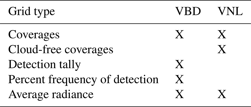
In 2015, EOG developed a nightly VBD data product optimized for offshore vessel detections (Elvidge et al., 2015a). VBD uses a DNB spike detector to identify offshore lighting and two additional indices to rate the amplitude and sharpness of the spikes. VBD runs over clouds and does not record the cloud state for detection. Specialized modules adaptively raise the detection threshold to reduce false detection from moonlit clouds and specular reflectance of moonlight in lunar glint zones. EOG supplies nightly VBD to fishery agencies and other organizations, primarily in Asian countries. EOG also builds monthly and annual summary VBD grids, which differ from VNL products in five respects: (a) VBD temporal summary grids only cover offshore areas. (b) Average radiances only include pixels with DNB spike detections, with no dilution of the average from overpasses lacking detection. (c) With nightly VBDs, it is possible to calculate the percent frequency of offshore lighting detection. (d) The summary grid products include data from all lunar conditions. (e) VBD reports detections made through optically thin clouds.

This paper reports a new comprehensive mapping of offshore lighting spanning multiple years, primarily based on EOG's nightly VBD product. The global offshore lighting grids from 2012 to 2022 are available for download via links listed in Elvidge et al. (2024). In addition, three papers have reported preliminary regional results from the VBD multiyear composite (Elvidge et al., 2023a and b; Chatterjee, 2023).

2 Methods

2.1 VIIRS boat detection data

In 2015, the Earth Observation Group developed the VBD algorithm with support from NOAA's Joint Polar Satellite System (JPSS) proving ground program and the U.S. Agency for International Development (USAID). The arrival of new DNB granules triggers VBD processing in near real time, with data distributed to several fishery agencies and other organizations. In Asia, the nightly VBD record extends back to April 2012. The global VBD record begins in 2017. VBD primary products include nightly .csv and .kmz files. A database has been built and is used to make global temporal composites and temporal profiles from individual features.

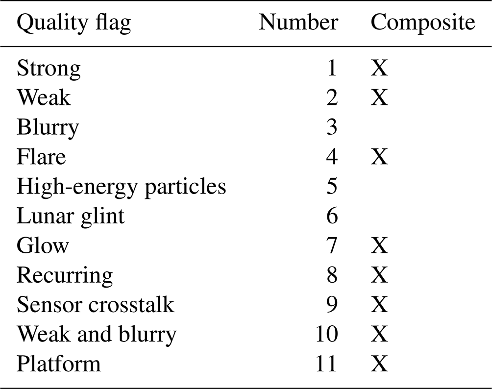
The VBDs are binned into 11 classes called quality flags (QFs), based on the DNB spike height, sharpness, and location (Table 1). The flare quality flags are defined based on EOG's infrared emitter catalog (Elvidge et al., 2023c).

When moonlight is either absent or extremely dim (less than or equal to 0.0001 lux), the spike median index (SMI) thresholds are set at a constant level for each detector aggregation zone. These thresholds are set slightly above the noise floor. This results in a stepwise increase in thresholds moving from the nadir to the edge of the scan. When moonlight is present, these low thresholds result in vast numbers of false detections from moonlit clouds. To address this problem, EOG developed a method for adaptively raising the SMI detection threshold to minimize the number of false detections. This adaptive thresholding is performed with the cross-correlation of the DNB image versus longwave infrared imagery band 5 (I5). A separate VBD module identifies zones where lunar glint is possible and adaptively sets detection thresholds to exclude DNB spikes associated with specular reflectance from the sea surface. The quality flags for flares are defined based on EOG's infrared emitter catalog (Elvidge et al., 2023c).

Table 1 VBD types.

2.2 Multiyear VBD composite

Four types of multiyear (2012–2022) 15 arcsec composite grids were generated from the VBD database: coverages, detection tally, average radiance, and percent frequency of detection. The detection tally and average radiance included VBDs from quality flags 1, 2, 4, 7, 8, 10, and 11. The set includes three sets of detection types with lower-amplitude DNB spikes, i.e., weak, glow plus weak, and blurry. Their selection is based on their spatial features matching VBD open-ocean density boundaries present in multiyear composites of the strong QF1 detections. For East and Southeast Asia, the multiyear composite has VBD data from 2012 to 2022. Outside of Asia, the composite has VBD data from 2017 to 2022. VBD follows the sparse style of grid filling (Fig. 1), where only the grid cell with the detection pixel center location is filled in (Elvidge et al., 2023c).

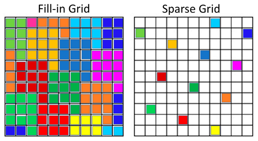
Figure 1 Fill-in and sparse geolocation for VIIRS pixels from a portion of a single sub-orbit into a 15 arcsec grid. The colors represent the pixel identities. In sparse gridding, only the 15 arcsec grid cells containing the latitude and longitude of the VIIRS pixel center are filled in. The fill-in style of geolocation starts from the sparse grid, followed by nearest-neighbor resampling to ensure all the grid cells are filled. From Elvidge et al. (2023c).

2.3 Multiyear VNL composite

A second 15 arcsec VNL composite was generated by merging 11 years (2012–2022) of VNL average DNB radiance grids with a background masked to zeroes. The methods used to make each of the annual VNLs are standardized (Elvidge et al., 2022). The 11 years of VNLs were downloaded from https://eogdata.mines.edu/products/vnl/#annual_v2 (last access: 27 January 2025). A land–sea mask is applied to the multiyear average and used as one of the depictions of offshore lighting. The VNL follows the fill-in grid approach shown in Fig. 1.

2.4 Comparison and potential merger of VBD and VNL composites

The offshore areas and feature content of the VBD and VNL composites are compared. The two sets of grids differ from each other (Table 2), but both contain average radiance. We evaluate whether combining the two based on average radiance would create a more comprehensive global map.

Table 2 VBD versus VNL summary grids.

2.5 Temporal profiles

We built the capability to extract nightly and monthly VBD temporal profiles based on vector polygons for specific cluster features, including fishing grounds, platforms, gas flares, and anchorages.

2.6 National offshore lighting index

The percentage of offshore areas with lighting detected from 2012 to 2022 was calculated for each country by dividing the lit surface, from the merged VBD and VNL grid, by the total offshore area calculated for that country's exclusive economic zone (EEZ).

3 Results

3.1 Comparison of VBD and VNL lighting areas

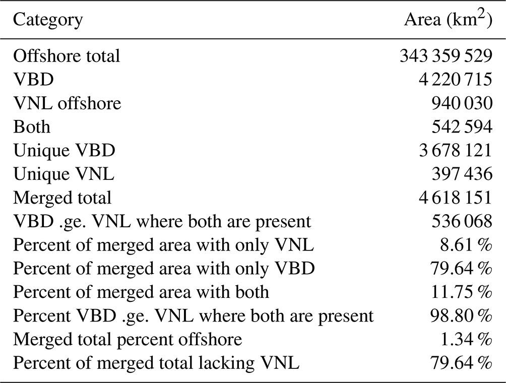
Four types of binary masks record the spatial extents of detections in VBD, VNL offshore, cells with both VBD and VNL, and grid cells where the VBD average radiance is greater than or equal to the VNL average radiance. The surface area under each binary mask is area-corrected to compensate for the reductions in 15 arcsec surface areas as a function of latitude. This makes it possible to report the area in square kilometers in Table 3. VBD covers 4 times more area than offshore VNL. The two products are meticulously merged (or blended) by taking the grid cell with the largest average radiance, ensuring the most accurate representation of the data extent. The merged total records the maximum extent of detected offshore lighting at 15 arcsec resolution. The percentage of the merged total with VNL only is 8.6 %. The rate of the merged area with VBD only is 79.6 %. The percentage of the merged area with detection in both VBD and VNL is 11.8 %. Where both VBD and VNL are present, VBD's average radiance is greater than or equal to (ge) the VNL radiance for 98.8 % of the area. The total area in the merged product covers 1.4 % of the offshore total. Note that VBDs are primarily point sources of lighting detected on individual nights, while VNL is a cloud-free average that incorporates DNB radiances when no lighting is present.

Table 3 VBD and VNL surface areas.

3.2 Side-by-side comparisons of VBD, VNL, and the merged set

On a global scale, VBDs cover 4 times more area than offshore VNLs. This section examines side-by-side examples of the two product sets as grayscale images and a color composite showing the blending. Figure 2 has VBD and VNL subsets for a fishing ground in the Arafura Sea in Indonesia. Land areas are marked dark green. The upper pair comes from VBD, with the percent detection frequency on the left and the average DNB radiance in the upper right. The most significant fishing ground extends south from Aru and has an elliptical cloud of detections that wraps around the island's southern tip. There is an empty buffer between the fishing ground and the shoreline, an expression of compliance with the government's ban on commercial fishing within 12 nautical miles of the shore (Indonesia, Central Government, 2025). The VNL set has the original multiyear average DNB radiance in the lower left with shoreline vectors. VNL has very few zones of onshore lighting in this part of the remote Arafura Sea. The masked VNL average DNB radiance is in the lower right. The VNL fishing ground features cover less area and have a blurry appearance compared to VBD. Fewer fishing ground detections allow for the averaging process of all-night, cloud-free observation. The sharpness appears blurry compared to VBD due to the differing methods used to fill the 15 arcsec grid. VBD takes a sparse grid approach, while VNL takes a fill-in grid approach (Fig. 1). The merged average radiance grid was sourced almost entirely from VBD, which has higher average DNB radiances than the corresponding multiyear VNL (Fig. 3).

The second example presents an area with a relatively even mix of VBD and VNL offshore lighting features – a portion of the Persian Gulf surrounding Qatar. Figure 4 provides a clear comparison, with the VBD set on top and the VNL set below. The VBD set includes the percent detection frequency in the upper left and the average radiance in the upper right. The VNL average DNB radiance image in the lower left has not been masked to zero out onshore lighting, making it easier to associate offshore glow with bright lighting present on the shore. Notably, lighting from gas flares in the Persian Gulf forms circular features in both VBD and VNL, with radiance tapering towards the outer edges. This practical example underscores the versatility of both VBD and VNL in different geographical settings.

Figure 5 is a color composite that reveals the source of the VBD–VNL merged product. The merged product reports the average radiance for the product with the larger average DNB radiance. The average radiance coming from VNL is red, and the average radiance from VBD is cyan. In the case of shorelines with glow, such as those of Qatar, Bahrain, and the United Arab Emirates, VNL was selected over VBD. This situation arises based on the specific characteristics of the glow and the spike detection nature of the VBD algorithm. VNL is also chosen in the gaps between sporadic VBDs in the glow surrounding flares. Note that EOG maintains a global catalog of gas flaring sites based on the infrared VIIRS Nightfire product (Elvidge et al., 2015b).

Key differences between the offshore VBD and VNL multiyear grids in the Persian Gulf include the following: (a) VBD has less glow detected than VNL surrounding bright lighting onshore, e.g., along the eastern shore of Qatar. (b) VBD glow surrounding gas flares has a fragmented appearance, with many gaps between grid cells having VBD. (c) VBD missed the glow surrounding one of the large flares. (d) Many gas flares have a near-vertical (north–south) high average radiance stripe. For (a) and (b), the paucity of VBDs offshore from major cities and surrounding gas flares can be traced back to the spike detector used in VBD and the land mask bump-out that occurred midway through the VBD series production. For (c), the missing flare glow is a result of the flare being on a small island, which resulted in a land mask VBD bump-out that thoroughly covered the flare glow. For (d), a form of hysteresis called crosstalk causes a vertical alignment of bright VBDs to either side of a large gas flare. Gas flares are notable as the brightest objects recorded by the DNB. DNB crosstalk is a false detection method found at extremely bright point sources (typically gas flares) aligned perpendicularly to the scan direction.

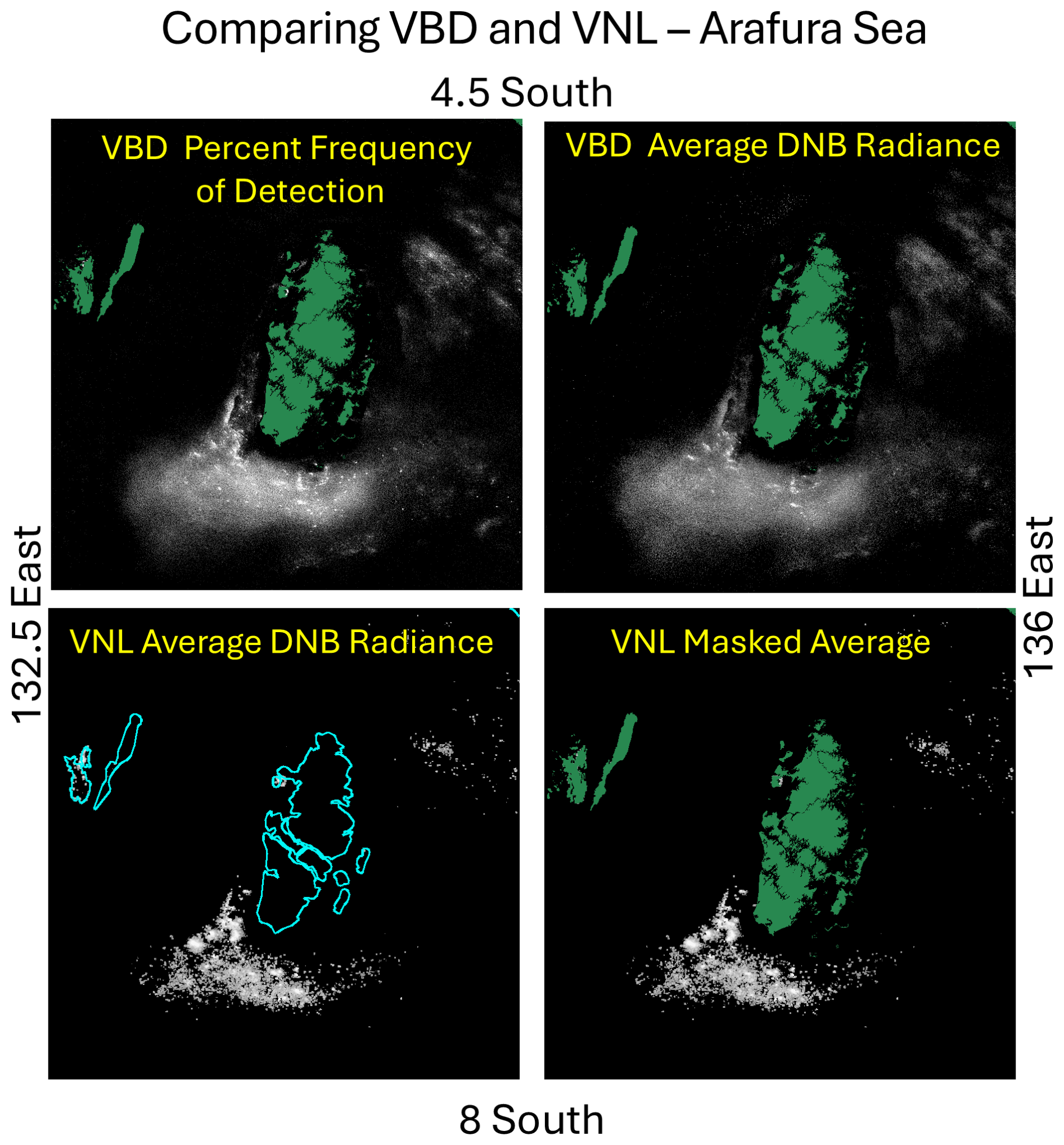
Figure 2 Comparison of VBD and VNL products for a fishing ground in the Arafura Sea, Indonesia. The VBD set includes the percent frequency of detection and the DNB average radiance. The VNL set consists of the original average DNB and the land-masked average radiance.

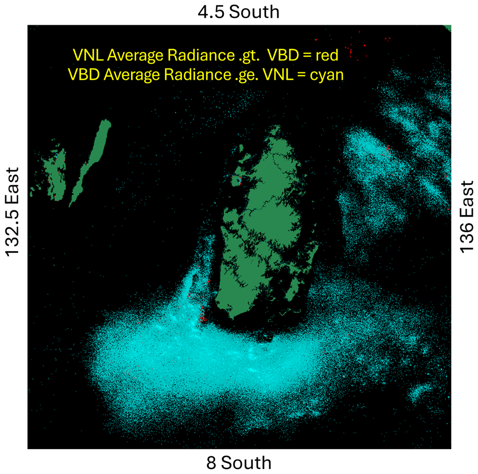
Figure 3 Combined VBD and VNL images of the Arafura Sea where the VNL average radiance exceeded VBD (in red) and where VBD exceeded the VNL radiance (in cyan).

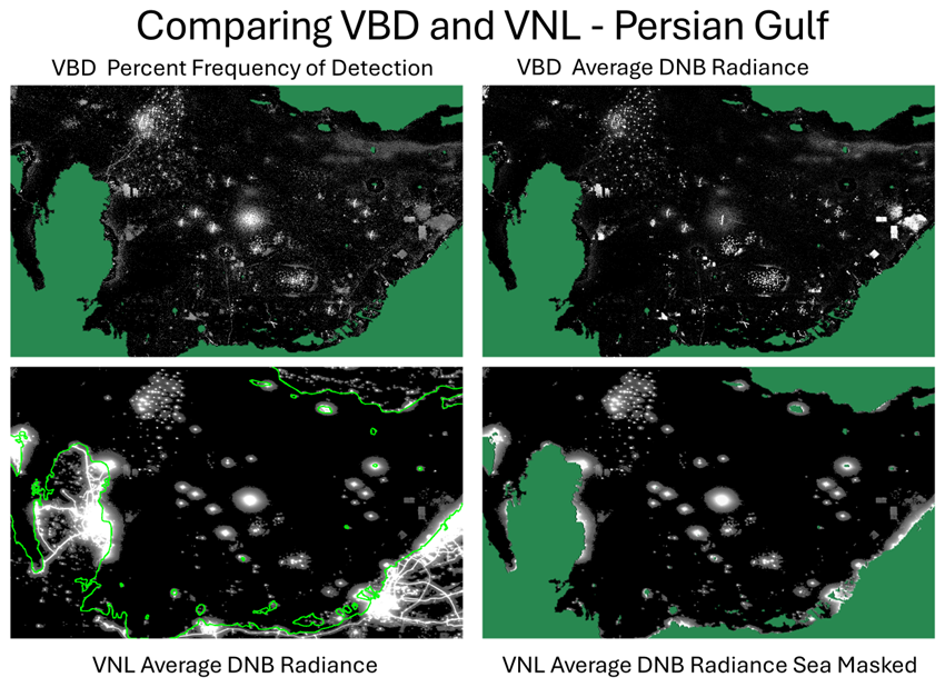
Figure 4 Comparison of VBD and VNL products for a fishing ground in a portion of the Persian Gulf surrounding Qatar. The VBD set includes the percent frequency of detection and the DNB average radiance. The VNL set consists of the original average DNB and the land-masked average radiance.

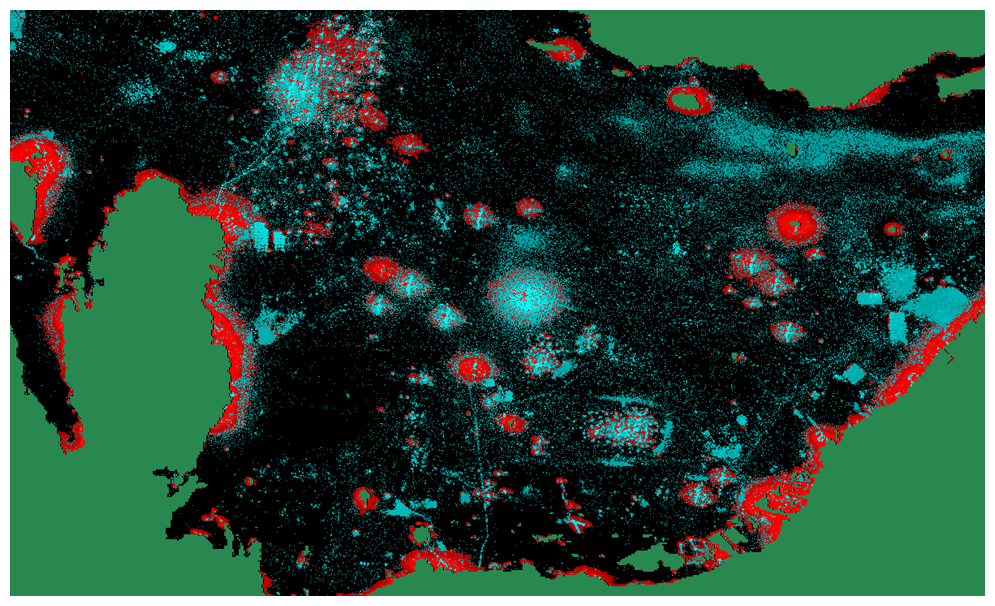
Figure 5 Combined VBD and VNL images of the Persian Gulf show where the VNL average radiance exceeded VBD (in red) and where VBD exceeded the VNL radiance (in cyan).

3.3 Offshore lighting structure types

Primary features identified in the VBD multiyear grids include diffused fishing grounds, recurring detections, lit platforms, gas flares, anchorages, and transit lanes. The lit platforms and gas flares are fixed-location facilities frequently evident in the monthly VBD composites. Fishing grounds and anchorage structures are incomplete in individual monthly composites, and their full extent may take multiple years to emerge. In this section, we examine features in the multiyear VBD grid using sample images from several parts of the world.

3.3.1 Diffused fishing grounds

Fishing ground features range from amorphous clusters of VBDs to boundary-constrained clusters. Figure 6 shows an amorphous fishing ground in the Arafura Sea. An empty buffer surrounding the main island is associated with the government's ban on commercial fishing within 12 nautical miles of the shore. There is a sharp vertical line, with a higher percentage frequency of detection on one side, located on the southwestern side of the main island. This may be related to the relaxation of the 12 nautical mile boundary at some point in the temporal record. There is a second fishing ground to the northeast of Aru. This fishing ground consists of a loose cluster of detections with a “salt-and-pepper” appearance. Similar examples of diffused fishing grounds have been identified in many parts of the world. The amorphous outline of the fishing grounds suggests that populations of catch species define the spatial extents.

3.3.2 Recurring detection sites

Individual 15 arcsec grid cells within amorphous fishing grounds typically have low-percentage detection frequencies – generally under 1 %. In shallow waters, there is often a random scattering of grid cells, with 2 % to 5 % detection frequencies referred to as “recurring detections”. Figure 6 shows an example of recurring detections from the Arafura Sea. There is something special about those grid cells, which boosts their percent detection frequency compared to their surroundings. However, the exact causes of the detection frequency boost have not been determined. Possible options include fish-aggregating device (FAD) locations on buoys, lift-net platforms, or floating service centers.

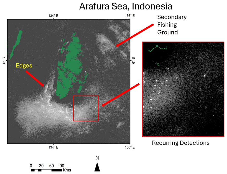
Figure 6 VBD percent detection frequency for fishing grounds in the Arafura Sea, Indonesia. The more considerable fishing ground is south of Aru – with a diffused “salt-and-pepper” pattern with detection density tapering at the edges. In addition, conspicuous grid cells have more significant percent detection frequencies – referred to as recurring detection sites.

3.3.3 Grids and linear recurring detections

This type of fishing ground is recognized based on grids or linear features with regularly spaced “anchor” grid cells with a substantially higher percentage frequency of detection. The individual anchor points are similar to the recurring detections found in amorphous fishing grounds regarding appearance and percentage detection frequency. However, the anchor cells are on evenly spaced grids and lines. The best examples of grid fishing grounds are in the Thailand EEZ, especially in the Gulf of Thailand (Fig. 7). The Thailand side of the gulf has an unusual regular grid pattern with 1 nautical mile spacing and is aligned north–south and east–west. The anchor grid cells have many more detections than their surroundings. Speculatively, this grid pattern may have been developed to deescalate conflict in fishing ground utilization and is self-organized by large fishing companies. The precise origin of the grid remains to be determined. The Fig. 7 inset image in the lower left shows the grid pattern near the island of Koh Tao. The island's government banned commercial fishing near the shore, and the width of this buffer zone was expanded midway through the VIIRS record, resulting in a double ring in the VBD numbers. The second inset image shows the junction between Vietnam, Thailand, and Malaysia. The Vietnam waters show a salt-and-pepper detection pattern with no indication of grids or linear clusters. On the Thailand side, the grid pattern typical of the north begins to transition to linear features near the Malaysian EEZ line. On the Malaysia side, east–west-oriented strings of evenly spaced grid cells with high VBDs are distinct from the grid pattern commonly found in Thailand waters and the random vessel detection pattern typical in Vietnam waters.

Figure 7 VBD percent detection frequency for portions of the Andaman Sea and Gulf of Thailand. The insets show the grid pattern common to many of Thailand's offshore fisheries. The center grid cells have 20 to 50 times more detections than the adjacent cells. In Thailand, many grids align with the cardinal directions, and the spacing between the grid centers is 1 nautical mile. Approaching the Malaysian EEZ line, the grids morph into diagonals. On the Malaysian side, there are east–west lines of equally spaced anchor grid cells with high numbers of VBDs.

3.3.4 Fishing grounds with artificial boundaries

There are several fishing grounds where the density of fishing boat activity changes abruptly along a line, indicating an artificial linear boundary. Some of these are EEZ boundaries, but others indicate boundaries established in bilateral agreements granting one country's fishing fleet authorization to fish in another country's waters (Amin et al., 2022). Several examples are present in the seas surrounding Japan, South Korea, and China. Figure 8 has a sharp set of boundaries not aligned with EEZ lines. The lines are inside the South Korean EEZ and the Japan–Korea Joint Use Area. Chinese fishing boats have authorization to fish up to the vertical lines in the middle of the zones. The density of fishing boats is higher on the western side of the lines, where Chinese fishing boats are permitted. The density of VBD is highest along the line's edge as fishing boats use lights to attract catch from over the line.

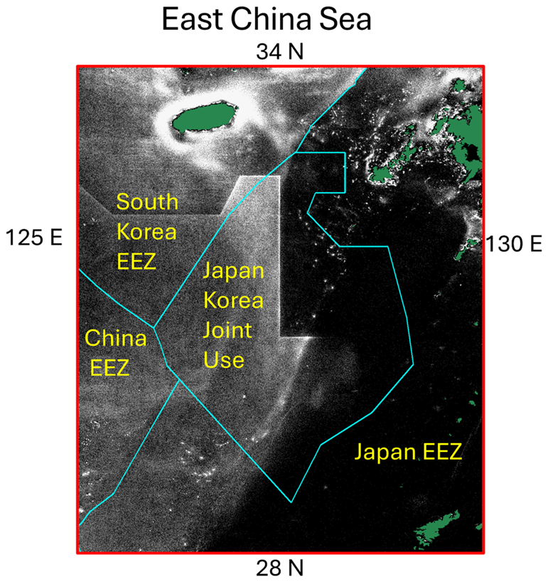
Figure 8 Multiyear VBD percent frequency of detection southwest of Japan. The EEZ boundaries are in cyan and labeled in yellow. Distinct linear features cross the South Korean EEZ and the Japan–Korea Joint Use Area. These boundaries are where the percent frequency of detection changes along a sharp boundary not aligned with the EEZ lines. These trace back to bilateral agreements granting Chinese fishing boats authorization to fish inside other EEZs.

3.3.5 Fishing grounds with convoluted boundaries

Several fishing grounds have distinctly convoluted boundaries. One example of this is offshore from Palawan in the southwestern Philippines (Fig. 9). Similar convoluted patterns can be found, but the one in Fig. 9 is exemplary. The origin of the convoluted patterns may be traced back to bathymetry, ocean currents, or other as yet unidentified reasons.

Figure 9 Multiyear VBD percent detection frequency surrounding the northern end of Palawan in the Philippines. The fishing grounds have sharp, convoluted edges.

3.3.6 Anchorages

These are not just compact clusters of VBDs: they are unique areas with linear edges or rectangular outlines found near ports and narrow sea passages with heavy vessel traffic. Vessels wait in anchorages to enter port or transit a sea strait. Anchorages stand out based on their higher-percentage VBD frequency than their surroundings. Anchorages near Singapore are shown in Fig. 10, and examples in the Bohai Sea (China) are shown in Fig. 11. The largest anchorages near Singapore are to the east and have sharp boundaries and several low-VBD transit lanes, a distinct feature of this area. Smaller bright patches on the Malaysian side of the Strait of Malacca are likely anchorages, another unique characteristic. There are rectangular and linear fishing grounds east of peninsular Malaysia, a pattern not commonly seen in other areas. Further east, there are bright spots in Indonesia's Natuna Sea, perhaps from lift-net platforms using lights to attract catch, a unique fishing method. The Bohai Sea area of China (Fig. 11) has many offshore lighting structures, including many anchorages, platforms, flares, and linear transportation tracks, a unique combination. The Bohai Sea has some of the largest anchorages in the world, which is a significant fact.

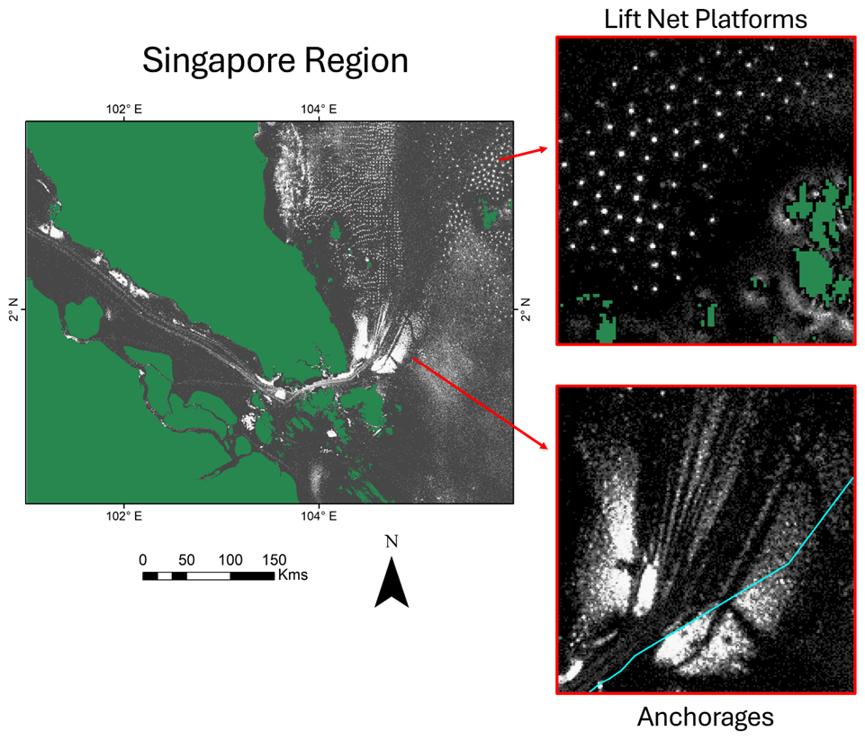
Figure 10 Multiyear VBD percent frequency of detection surrounding Singapore. The area has multiple anchorages east of Singapore and several smaller anchorages on the Malaysian side of the Strait of Malacca. Fishing grounds are present to the east of peninsular Malaysia.

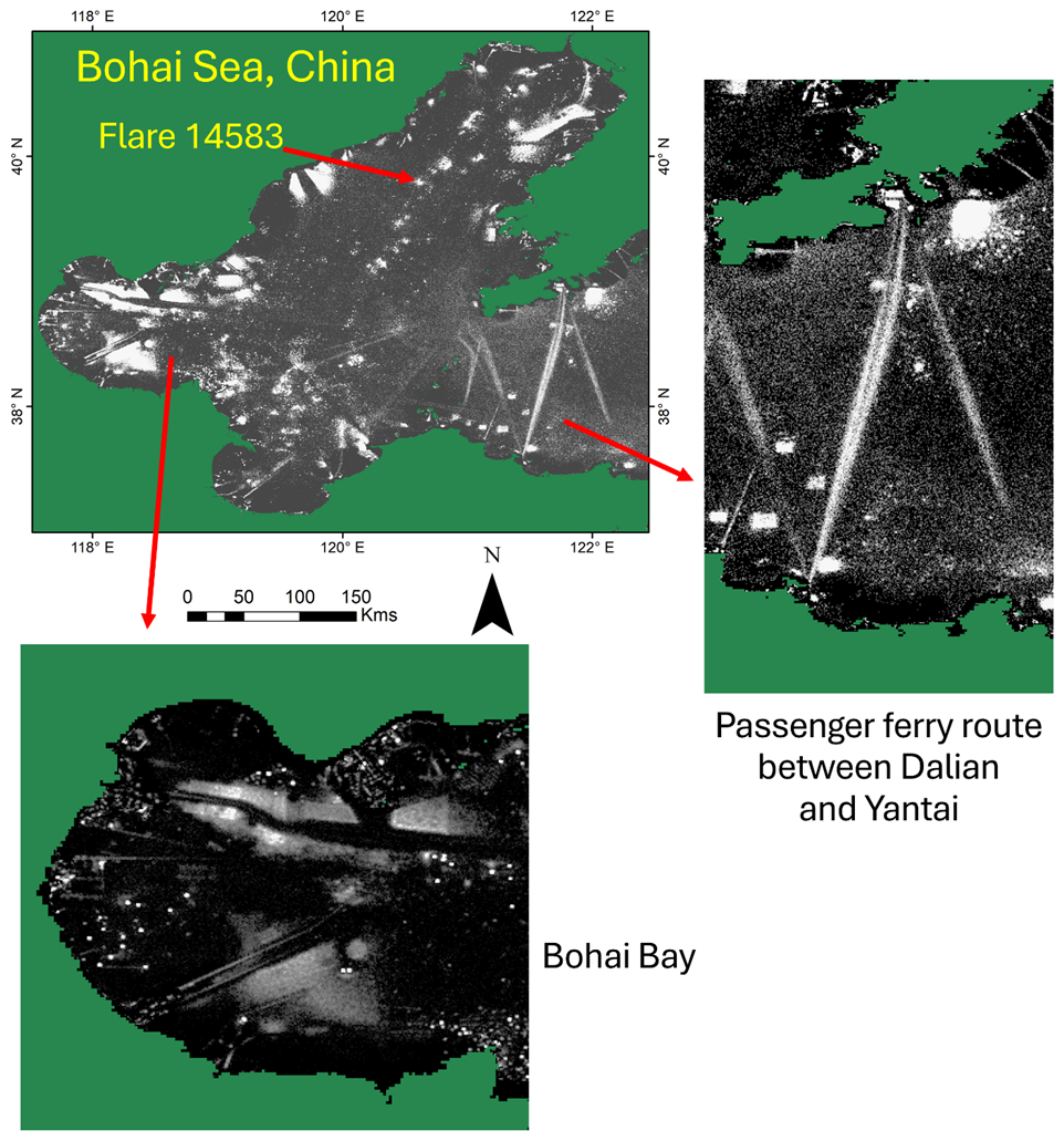
Figure 11 Multiyear VBD percent frequency of detection in the Bohai Sea of China. The area has multiple anchorages, platforms, and transit lanes.

3.3.7 Transit lanes

The best examples of VBD transit lanes are passenger ferry tracks going from one port to another. Figure 11 shows several examples in the Bohai Sea VBD image. The Mediterranean Sea is another area with many passenger ferry tracks. Shipping lanes can have sparse tracks in the multiyear VBD composite, such as the sparse tracks through the Strait of Malacca in Fig. 10. Another type of transit lane present in the multiyear VBD product is air transit routes, including stacked routes over the North Atlantic Ocean. The air transit routes arise from VBDs from moonlit aircraft.

3.3.8 Cat eyes

The cat eyes phenomenon, a unique offshore lighting feature, is a fascinating blend of atmospheric scattering of light surrounding large flares and a DNB sensor artifact known as “crosstalk”. This intriguing phenomenon has been studied since the mid-1970s, when it was discovered that large gas flares have distinct glow haloes in low-light imaging visible band data collected by DMSP satellites at night (Croft, 1979; Elvidge et al., 2009). Glow haloes surrounding natural gas flares are also observed in the VIIRS DNB, as seen in the Persian Gulf in Fig. 4. In addition to the atmospheric glow surrounding large flares, there is a DNB feature called crosstalk. This phenomenon, a hysteresis effect (Mills, 2016; Mills and Miller, 2016), results in signal leaks from extremely bright DNB pixels containing flares to an along-track set of pixels from the same scan. The affected pixels have much higher radiances than the surrounding areas but lower radiances than the flare pixel. Crosstalk accumulates in the multiyear VBD composite as a slit-like bright feature surrounded by a circular glow pattern – forming a feature reminiscent of a cat's eye (Fig. 12). The multiyear VBD composite excluded the VBD label “crosstalk” from the near-real-time nightly products. The current crosstalk identification is based on a vector polygon set drawn in a limited-duration temporal composite from the 2015–2016 time range. The nightly labeling of crosstalk is incomplete, indicating that the vectors should be redrawn based on the new multiyear composite.

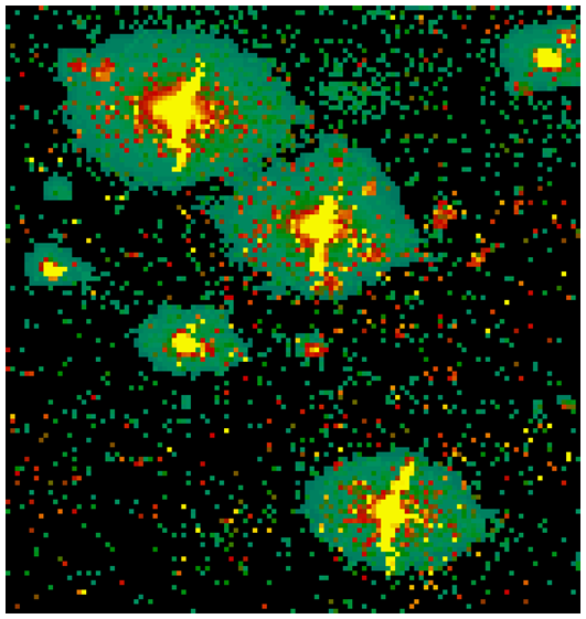
Figure 12 Cat's eye features are found in the merged VBD and VNL composite in the Persian Gulf (subset from Fig. 4). The green features are from the visible glow of scattered light surrounding large gas flares. The DNB crosstalk is a hysteresis effect where radiance leaks to pixels with the same sample number from individual 16-line scans collected by VIIRS.

3.4 Temporal profiles

The individual nightly VBDs are in a database – making it possible to extract nightly temporal profiles based on vector polygons established for individual lighting structures. Figures 13–14 have examples of VBD fishing ground temporal profiles. As noted by other authors, VBD fishing grounds have distinct annual cycling. The Arafura fishing ground (Fig. 13) shows steady increases in detections each year from 2012 to 2019, followed by declines in 2022–2023. The Myanmar fishing ground (Fig. 14) also has conspicuous annual cycling and remained steady from 2012 to 2023. The Singapore anchorages (Fig. 15) have no annual cycling but relatively steady nightly detection numbers from 2012 to 2020. There are two periods – in 2016 and 2020 – where detection numbers increased to nearly 100 per night. The anchorage detection numbers dropped in 2021 and remained low through 2023, possibly indicating a supply chain slowdown. The gas flare in the Bohai Sea (Fig. 16) shows largely steady activity from 2012 to mid-2015, followed by 5 years (2016–2020) of reduced flaring activity and then increased flaring activity in 2022–2023. The nightly DNB radiance for the flare closely follows the nightly shortwave infrared radiance levels recorded by the VIIRS Nightfire product (Fig. 17). Electric lighting is rarely detected in the shortwave infrared, implying that the flare rather than the electric lighting dominates the DNB radiance at the site.

Figure 13 The nightly temporal profile of VBD tallies for the fishing ground south of Aru (Fig. 2). Each year, there is a decrease in the detection numbers from January to June, corresponding to the rainy season. The detection numbers increased consistently from 2012 to 2021 but declined in 2022 and 2023.

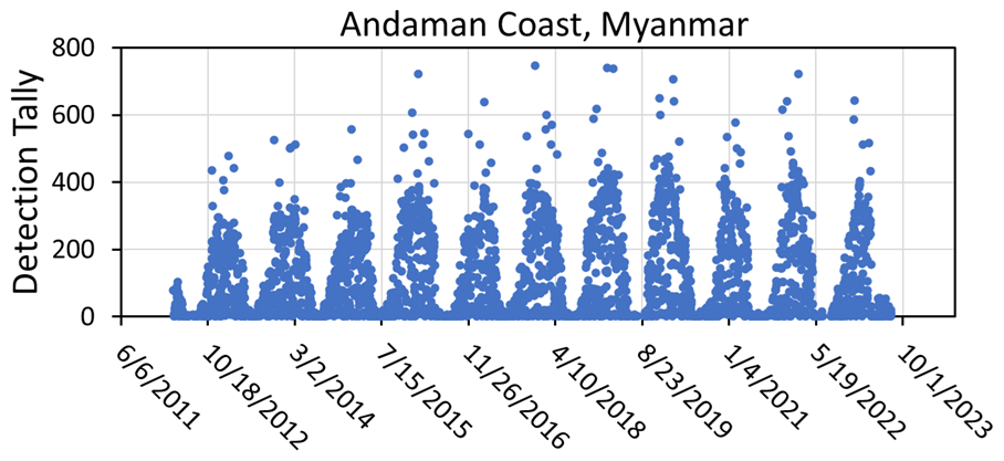
Figure 14 VBD tally temporal profile for the Myanmar fishery along the Andaman coast. The profile shows vigorous annual cycling, with low detection numbers during the monsoon months (June through September). There is a gradual increase in yearly detections from 2012 through 2020, and then they are near steady from 2021 through 2022.

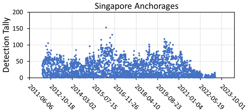
Figure 15 VBD tally temporal profile for the Singapore anchorages, as shown in the inset image of Fig. 9. The anchorage boat detection tallies were 50 to 70 per night in 2012 and increased to 100 detections in 2017 and 2020. The detection numbers declined in 2021 and were down to 10–15 per night in 2023.

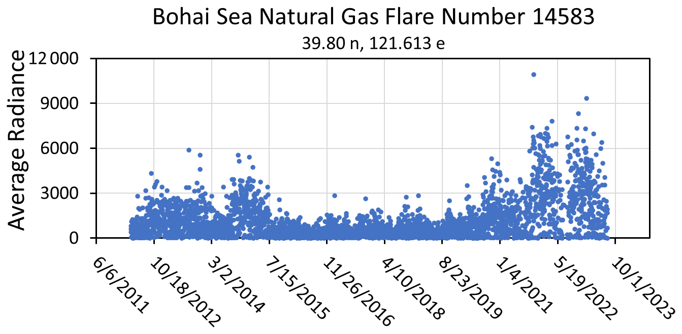
Figure 16 VBD radiance temporal profile for a natural gas flare in the Bohai Sea. The radiance ranges from 2500 to 3000 from 2012 to mid-2015. Then, the radiance declines to nearly 1000 from 2016 to 2020 before increasing again from 2021. The pattern closely matches the flare's shortwave infrared radiance profile from the VIIRS Nightfire time series (Fig. 17).

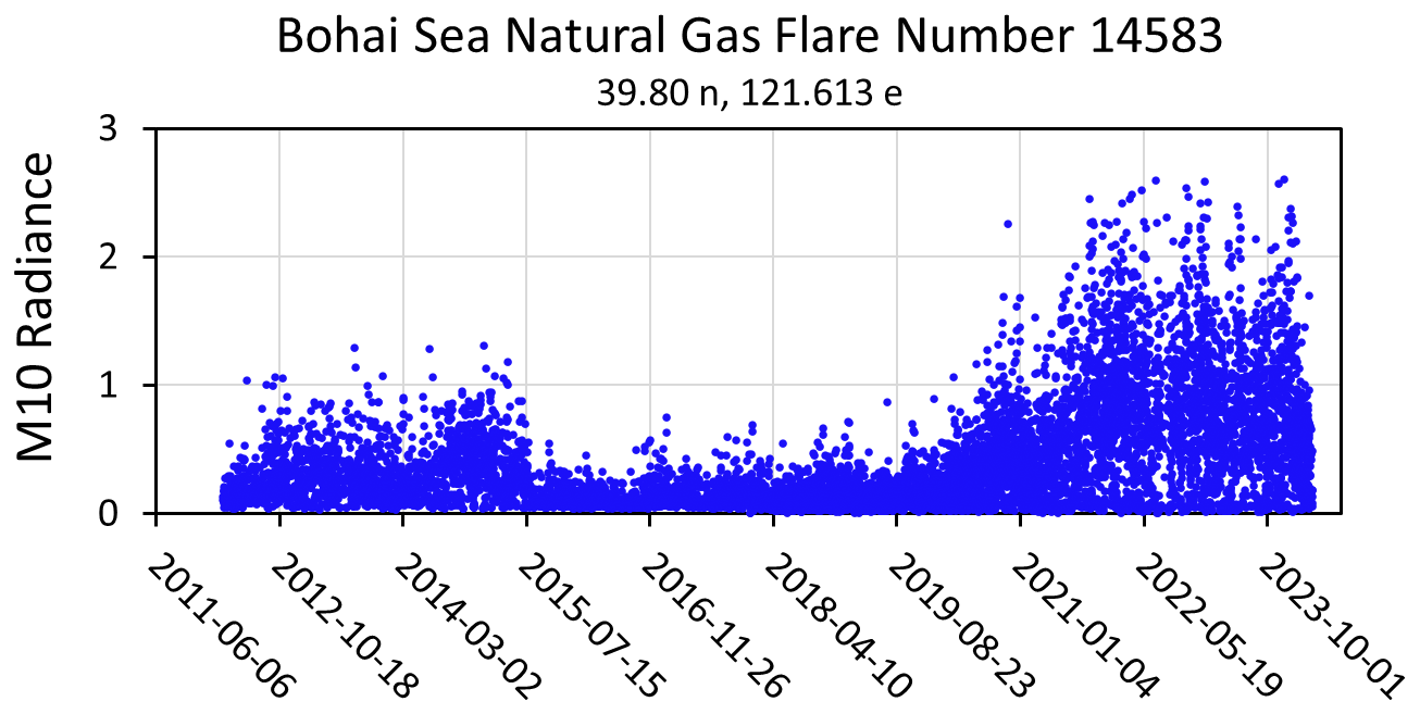
Figure 17 Nightly shortwave infrared (band M10) radiance (W m⁻² sr⁻¹ µm⁻¹) for the Bohai Sea natural gas flare from the VIIRS Nightfire product line. Because the DNB radiances closely track the M10 radiance levels, we conclude that the DNB radiance is dominated by the flare's radiant emissions and not the electric lighting at the site.

3.5 National rankings of the offshore lighting coverages

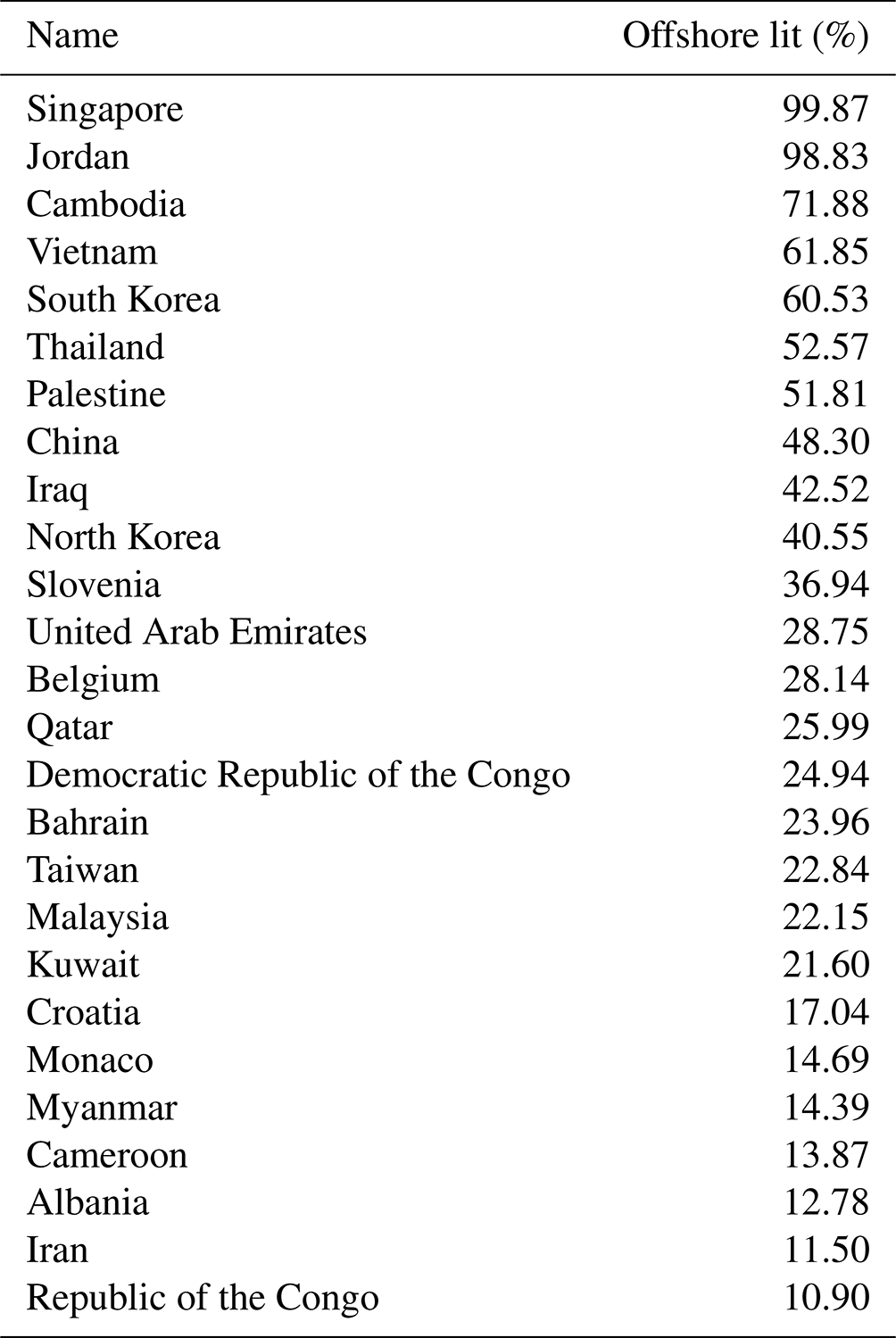
The spatial extent of offshore lighting in different countries' EEZs is calculated as a percentage and is listed in Table 4. The percentage of offshore lighting is the area of lit grid cells divided by the total EEZ area. This calculation method allows for an accurate comparison of lighting levels between different countries and regions, as it normalizes for each country's EEZ size. The surface area of each grid cell is adjusted to account for the decreasing sizes of grid cell areas as latitude increases. The resulting percentages provide valuable insights into the extent of offshore lighting and its potential impact on marine ecosystems. Singapore has the highest percentage, with nearly 100 % of its EEZ showing detected lighting. Jordan follows with a small portion of the Gulf of Aqaba, an arm of the Red Sea. Asian countries, such as Cambodia, Vietnam, South Korea, and Thailand, also show significant spatial extents for offshore lighting. Note that the percentages are based on tallies of lit 15 arcsec grid cells and represent areas impacted by artificial lighting. The actual area of lighting (luminaires) is quite small but is readily visible from a considerable distance at sea.

Table 4 Rankings of countries based on the percentage of EEZs with VIIRS-detected lighting.

4 Discussion

Users should be aware of several critical differences between the VBD and VNL multiyear composites. While both product suites include an average radiance, this is calculated differently and is not directly comparable. VBD calculates its average radiance by summing the radiances of VBDs in each grid cell and dividing them by the number of detections. It operates without cloud screening and utilizes data from all lunar phases. On the other hand, the VNL's average radiance is derived from the cloud-free DNB radiances from dark portions of lunar cycles, divided by the number of cloud-free observations. The VNL products are filtered annually to remove outliers, and the backgrounds are zeroed out. These distinct characteristics play a significant role in their respective applications.

The VBD multiyear composite stands out by including the percent detection frequency grid, which VNL does not provide. This metric is possible in VBD due to the spike detector at the algorithm's core. While VNL averages cloud-free observations, it does not track the number of times lighting is detected and thus has no calculation of the percent frequency of detection.

The VNL long-term composite excels in depicting the offshore glow surrounding bright sources. However, it falls short in detecting lit fishing boats due to the outlier removal step that filters out biomass burning on land. In contrast, VBD readily detects isolated lit pixels embedded in dark backgrounds, providing a more complete depiction of fishing ground spatial extents and temporal profiles. This clear distinction between their strengths and limitations can guide readers in choosing the most suitable grid for their specific needs.

Regarding the area results presented in Tables 3 and 4, it is important for the user to recognize that these are based on tallies of 15 arcsec grid cells with offshore lighting detected. The actual lighting area is limited to the luminaires and is minuscule compared to the image grid cells. The 15 arcsec grid cell tallies represent the ocean surface area affected by artificial lighting on one to many nights during the 11-year compositing period. We included a latitude-based area correction to avoid exaggerating lit area sizes at higher latitudes.

5 Data availability

The multiyear VBD, VNL, and merged grid sets are available in Elvidge et al. (2024; https://doi.org/10.25676/11124/179157).

6 Conclusion

At night, the ocean's surface is a vast dark palette where the VIIRS day–night band can readily detect faint lighting sources. While EOG produces VBD nightly, the nightly products do not exhibit the sharply defined structures depicted in Figs. 2–11. Fixed locations, such as lit platforms, are able to propagate to the monthly VBD composites. However, more extended periods of temporal compositing are required to reveal the full spatial extent of fishing grounds, anchorages, and transit lighting structures. Where vessels are transitory, lighting structures emerge through the accumulation of detections over multiple years.

The multiyear offshore lighting products were initially developed to identify fishing grounds for labeling VBDs from fishing boats. The development effort was our response to Philippine and Indonesian fishery agency staff who asked us how to distinguish lit fishing boats from other sources of offshore lighting. They noticed that there are numerous VBDs in locations not known to be fishing grounds. To answer the question, we accumulated VBDs across Southeast Asia over extended periods of time and found that the fishing grounds emerged as loose clusters with numerous VBDs. In shallow waters, fishing grounds often have locations with many more detections than their surroundings, which are referred to as recurring detection locations. These may be lift-net platforms where light is used to aggregate catch. In the Gulf of Thailand, these recurring detection locations are arranged in regular grids. In Malaysia, the recurring detections are often arranged in regularly spaced lines. This mapping makes it possible to distinguish light detections from fishing boats from other sources.

Based on the features found in the regional prototype, we embarked on an effort to assemble a comprehensive global mapping of offshore lighting. VBD is quite good at detecting isolated sources of lighting but does poorly in detection of glow along shorelines and bright offshore sources. To make the product comprehensive, we combined VBD with the offshore portions of EOG's VNL product. VNL is designed for annual mapping of onshore lighting from human settlements and includes the glow along shorelines and bright offshore sources.

Taking this approach, we have produced a comprehensive mapping of offshore lighting structures using a combination of two global VIIRS multiyear nighttime light products – VBD and VNL. Large numbers of distinct features are evident, which we refer to as lighting structures because they have defined shapes and locations. Overall, VBD has vastly more identifiable lighting structures but is depauperate in glow. The two products are merged at the grid cell level by accepting the product with the higher average radiance. We provide open access to the VBD and VNL products separately as well as the combined product, so that users can use the one they prefer.

To increase the value of the offshore lighting product, we plan to generate bounding vectors and temporal profiles for many more offshore lighting structures and give each structure a source type (e.g., fishing ground, anchorage, or flare) plus a unique identification number. This will make it possible to label the individual VBDs in the nightly VBD product with their type-associated feature number. We also plan to derive temporal profiles for as many of the lighting structures as possible, in order to periodically update the temporal profiles and provide access via a web map service. We will also work to improve the quality of the multiyear offshore lighting product by fully reprocessing the source data with a new cloud detection algorithm and an atmospheric correction.

The current product set provides the most comprehensive mapping to date of offshore light pollution. The examples presented in this paper's figures barely scratch the surface in terms of the vast numbers of interesting offshore lighting features revealed in the data product. We expect the data to be useful in marine spatial planning, improved delineation and analysis of fishing grounds, and supply chain issues embedded in the anchorage temporal profiles.