The OCEAN ICE mooring compilation: a standardised, pan-Antarctic database of ocean hydrography and current time series

Continuous moored time series of temperature, salinity, pressure and current speed and direction are of great importance for understanding the continental shelf and under-ice-shelf dynamics and thermodynamics that govern water mass transformations and ice melting in and around Antarctic marginal seas. In these regions, icebergs and sea ice make ship-based mooring deployment and recovery challenging. Nevertheless, over decades, expeditions around the fringe of Antarctica sporadically deployed and recovered hundreds of moored instruments, including those facilitated through ice shelves boreholes. These datasets tend to be archived in a wide range of data centres, with, to our knowledge, no clear format standardisation. As a result, systematic analysis of historical mooring time series in the marginal seas is often challenging. Here we present the first version of a standardised pan-Antarctic moored hydrography and current time series compilation, with broad international contributions from data centres, research institutes and individual data owners. The mooring records in this compilation span over five decades, from the 1970s to the 2020s, providing an opportunity for a systematic study of the pan-Antarctic water mass transport and shelf connectivity. As a demonstration of the utility of this compilation, we present spectral analysis of the compiled current velocity time series, which unsurprisingly shows the dominating presence of tidal variability within most records. This component of the variability is fitted using multi-linear regression to tidal frequencies, and the tidal fit is removed from the original time series to leave de-tided variability. Given the limited record durations to months to years, de-tided variability is dominated by synoptic (3–10 d period), intraseasonal (10–80 d) and seasonal (∼6 months–1 year) signals. The spatial distribution of the kinetic energy integrated within frequency bands is presented and discussed within respective regional contexts, and future avenues of research are proposed. This data compilation is assembled under the endorsement of Ocean-Cryosphere Exchanges in ANtarctica: Impacts on Climate and the Earth System (OCEAN ICE) project (https://ocean-ice.eu/, last access: 23 October 2025) funded by the European Commission and UK Research and Innovation. It is available and regularly updated in NetCDF format with the SEANOE database at https://doi.org/10.17882/99922 (Zhou et al., 2024a).

1 Introduction

The Antarctic continental shelves host multiple sites of unique water mass formation: coastal polynyas are the site of intense ocean heat loss to the cold polar atmosphere, freezing the sea surface and via brine rejection creating dense salty waters known as High Salinity Shelf Water (HSSW). In some parts around Antarctica, further heat loss via interaction with the Antarctic ice sheet creates supercooled, saline water masses, known as Ice Shelf Water (ISW), which, together with HSSW, form the precursors of the most voluminous water mass, Antarctic Bottom Water, that fills the global abyssal ocean (Richardson et al., 2005; Li et al., 2023). Closer to the surface, freshwater resulting from sea ice and ocean-driven glacial melt of the ice sheet modulates the interactions between atmosphere, ocean and sea ice (Richardson et al., 2005; Bronselaer et al., 2018; Haumann et al., 2020). It also modifies exchanges between adjacent seas (e.g., Jacobs et al., 2022) and with the Southern Ocean, as the slope current and front associated with lateral gradients of temperature and salinity form a dynamic cross-shelf barrier (Thompson et al., 2018). Through turbulent mixing and modulation of source water properties, shelf sea processes impact the deep ocean ventilation. These processes influence climate by setting the strength and properties of the overturning circulation and the exchange of heat and moisture with the atmosphere. Capturing the processes governing the formation and transport of these water masses is challenging using observations due to logistical difficulties for ships to access these regions readily. As a result, our knowledge of the freshwater budget over the Antarctic continental shelves and Southern Ocean is poor, with important repercussions for climate modelling and sea level rise projections (Heywood et al., 2012).

Recent models and observations from a few locations (e.g. Han et al., 2022, 2024) have highlighted how tidal currents and topographic Rossby waves can promote the mixing and descent of dense water plumes along the continental slope. However, it remains unclear if these findings can be generalized to all dense water outflows. Similarly, the transport of glacial meltwater affects oceanic processes downstream, including ice shelf melting, sea ice formation and the creation of dense shelf waters, especially in the West Antarctic sector from the West Antarctic Peninsula to the Amundsen and Ross Seas (Nakayama et al., 2020; Jacobs et al., 2022; Dawson et al., 2022; Flexas et al., 2022). However, due to the lack of observations over most of the Antarctic continental shelf, little is currently known about the connectivity of the circum-Antarctic shelf seas with few exceptions in region near the Antarctic Peninsula (e.g., Thompson et al., 2009).

Here, we present the first version of a standardized compilation of historical moored time series that have been deployed over the past 50 years on the Antarctic continental shelves and slopes and present a rapid overview of energetic characteristics of ocean circulation on and off the continental shelves along with their hydrographic context. This compilation includes temperature, salinity, pressure and ocean current time series south of 60° S (Fig. 1a). The time series are freely and publicly accessible in a standardized format at SEANOE (https://www.seanoe.org/data/00887/99922/, last access: 23 October 2025, Zhou et al., 2024a). We intend to maintain and enhance the compilation on an annual basis and welcome contributions for inclusion in future releases. This mooring compilation is endorsed by the OCEAN ICE project funded by the European Commission and UK Research and Innovation, and we refer to this data compilation as the OCEAN ICE mooring compilation herein. This dataset aims to provide opportunities for regional or systematic pan-Antarctic studies on water mass transport, formation processes and shelf connectivity.

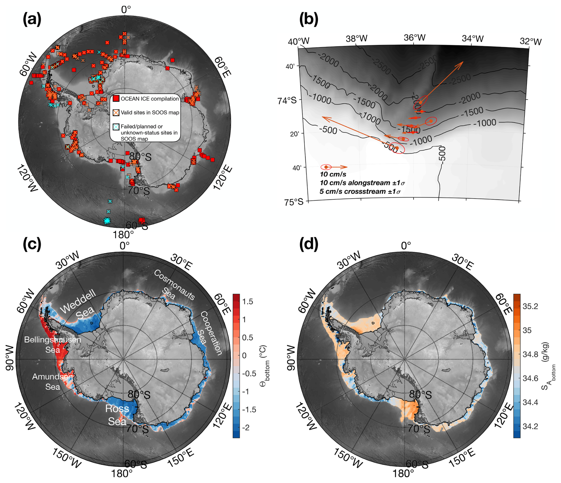
Figure 1 (a) A comparison between the OCEAN ICE moored time series compilation and Southern Ocean Observing System (SOOS, https://www.soosmap.aq/, last access: 12 September 2024) map metadata information. The SOOS mooring map information is retrieved from the SOOS map webpage by specifying the instrument type as “fixed platform” in the interactive webpage. Each square represents a record in either SOOS map or OCEAN ICE compilation. The red squares are those contained in the OCEAN ICE compilation. Hollow squares with orange crosses are valid sites in SOOS map (with status of recovered or deployed). The overlapping sites across the OCEAN ICE compilation and SOOS map are then denoted as a red square with an orange cross on top. Blue crosses are those sites in SOOS map that are shown as either planned, failed or unknown status. These sites are either invalid, or the data remains to be released. (b) An example of depth-averaged current vectors and the variance ellipses denoting the cross-stream and along-stream current variabilities for a group of shelf break moorings in the southern Weddell Sea (Darelius et al., 2023). (c) Bottom temperature and (d) bottom salinity over the continental shelf (<1000 m) is shown to distinguish different thermal regimes across the Antarctic continental shelves. Bottom properties are computed as the mean value over the bottom 150 m from the seabed from a climatology product constructed from the hydrographic profiles (Zhou et al., 2024b). Bathymetry, in grey shading, is from RTopo 2.0.4 (Schaffer et al., 2016). Bottom water properties shown in panel (c) and (d) are computed using TEOS-10 toolbox (McDougall and Barker, 2011).

2 Data sets and processing

2.1 Overview

In the OCEAN ICE mooring compilation, we collected 521 mooring time series, covering 470 deployment sites (Fig. 1a). The comparison with the Southern Ocean Observing System (SOOS, https://www.soosmap.aq/, last access: 12 September 2024) mooring map which aims at compiling links to datasets from all past endeavours shows that our compilation includes additional mooring records, e.g. in front of the Ross Ice Shelf and from instruments deployed through boreholes in the Ross and Amery ice shelves. More importantly, while the SOOS interactive map displays mooring locations with limited metadata (name, country, coordinates), it does not provide access to the underlying datasets or direct download links. In contrast, the OCEAN ICE dataset presented here offers direct access to the full time series. Therefore, the OCEAN ICE mooring compilation is an effort to improve spatial coverage and directly provide publicly available datasets, calling on experienced international collaborators to obtain a compilation that is as complete as possible. This effort will be continued, and the compilation will be expanded in future annual releases. At this stage, we have collated data from regions and features not represented in SOOS, including the Antarctic Slope Current and Antarctic Bottom Water transport over the slope current from places such as the southeastern Weddell Sea (Graham et al., 2013), Princess Elizabeth Trough (Heywood et al., 1998) and Australian-Antarctic Basin (Peña-Molino et al., 2016), in addition to those that have been logged in the SOOS map. The mooring time series are acquired from various sources. Some of them are archived in public databases such as Pangaea Data repository, British Oceanographic Data Centre, UK Polar Data Centre, US Antarctic Program Data Center, Australian Antarctic Data Centre, Korea Polar Data Centre, Norwegian Marine Data Centre and Norwegian Polar Data Centre. Others are stored in places that are less commonly considered as Antarctic mooring data centres such as NCEI/NOAA, or local databases hosted by individual institutes such as Lamont-Doherty Earth Observatory of Columbia University and Oregon State University (e.g. the OSU Buoy Group, https://cmrecords.net/history.html, last access: 29 May 2024). A list of mooring record source links is stored with our database and is available as an additional file on SEANOE where the OCEAN ICE mooring compilation is published. Figure 1b showcases a regional example of current meter measurements and some basic information, namely the depth-averaged current vectors along with variance ellipses depicting the along-stream and cross-stream velocity variabilities. The broad spatial spread of these mooring sites covers different thermohaline regimes over the continental shelves as indicated by the climatological bottom water temperature/salinity in Fig. 1c and d, from the colder and saltier dense water formation site of the Ross, Weddell, and Cosmonaut seas to the warmer Amundsen and Bellingshausen seas. One notable characteristic of this dataset is its typical mid-water column to near-seabed sampling bias. Indeed, most mooring deployed in Antarctic shelf seas tend to avoid sampling the near surface region where drifting icebergs can damage instrumentation, especially those mooring located south of 70° S where iceberg drift are more frequent (Fig. 2a). Some exceptions where the instruments were mounted close to the top of the water column at 75° S (Fig. 2a) lie in two sub-iceshelf moorings that were designed to measurement the turbulence processes in the ocean-ice boundary layer in George IV ice shelf (Middleton et al., 2022) and Larsen C ice shelf (Davis and Nicholls, 2019). Among 521 mooring timeseries, over 80 % of them have the capacity of measuring at least current velocities and temperature (Fig. 2a). The mooring timeseries typically have a good coverage over different seasons (Fig. 2b) mainly because most of the mooring timeseries last for a full year or more (Fig. 2c).

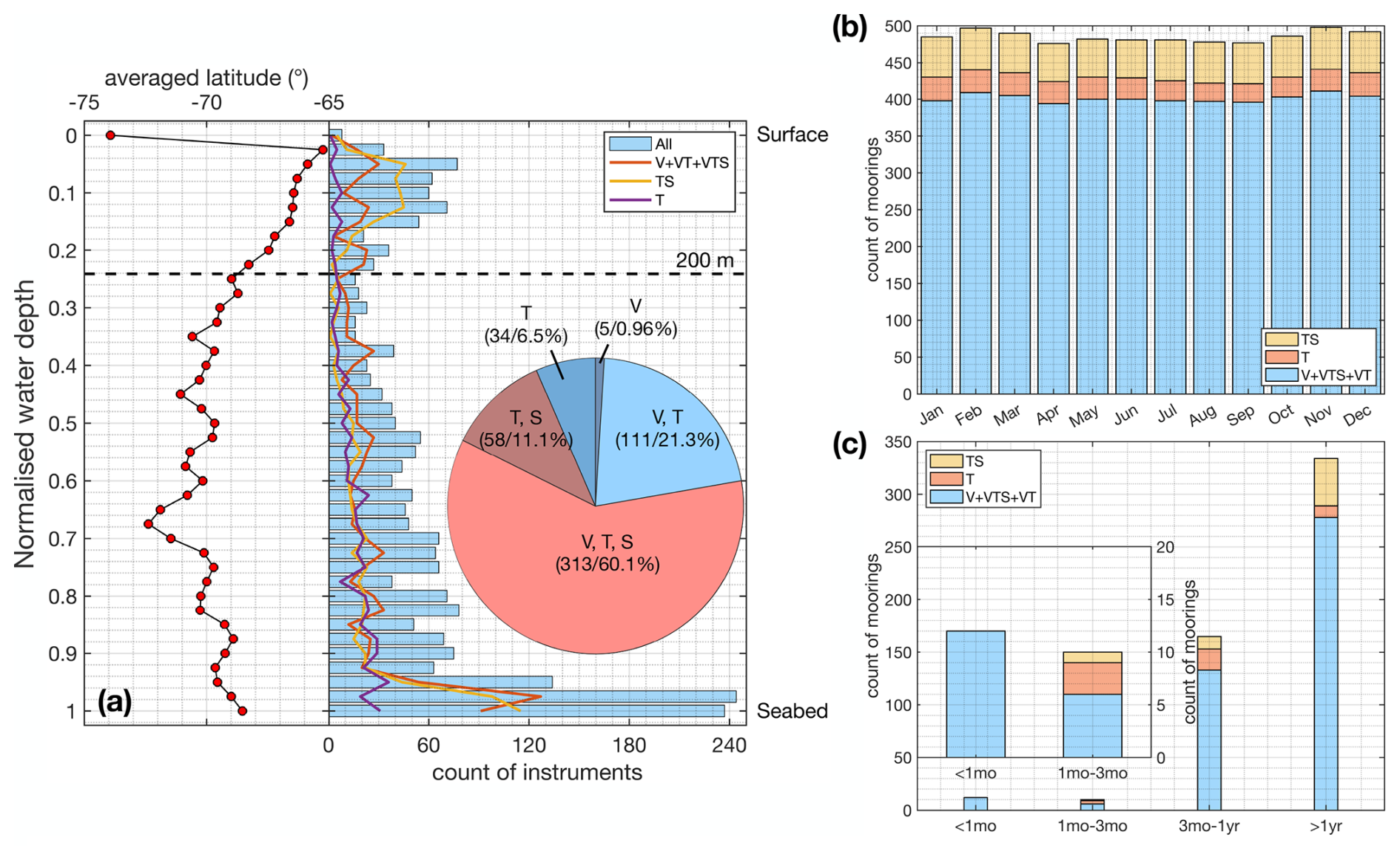
Figure 2 Overview of mooring compilation statistics on (a) instrument depths and location, inserted pie chart shows the measuring variables by all mooring compositions. 5 types of measuring variables combination are selected: VTS (current velocities, temperature, salinity), VT (current velocities and temperature), TS (temperature and salinity), T (temperature only), V (current velocities only). (b) easonal coverage of each type of measuring variable combination shown in the legend. (c) Same as (b) but for measuring period.

2.2 Data standardisation

All the mooring time series are standardized and re-formatted into individual NetCDF files for each mooring site, following a consistent file structure. The source of individual datasets is also provided, allowing further investigations and analysis of the processing steps applied to each time series before we obtained them. We are not always aware, for example, if corrections for current-induced motions of the sensors or the magnetic declination corrections on current direction have been applied for each individual mooring. To support assessment of data quality and provenance, we provide source links for each mooring dataset. These links direct users to original data landing pages, cruise or deployment reports, or data owners, where details on applied quality control flags and processing procedures can be obtained. Users are encouraged to consult these sources to evaluate the suitability of the data for their specific applications. For moorings containing multiple instruments, to acknowledge the fact that these instruments are sampled at different frequencies and over different periods of time, each instrument is accompanied by its own time vector in the NetCDF file. Table 1 shows examples of variable lists from three types of the most commonly deployed instruments – Temperature, Conductivity and Pressure logger (e.g., SBE37 MicroCAT), Acoustic Doppler Current Profiler (ADCP, e.g., Teledyne RDI 75 kHz ADCP), and current meter (e.g., Aanderaa Rotor Current Meter). Note that in the final form of the mooring file, we retain the original sampling frequency for all the mooring instruments as we received it (some were already processed and averaged), avoiding modifications of the temporal resolution as much as possible, to ensure broader use of these mooring records for analysing processes spanning sub-daily to interannual time scale ranges. Additionally, we performed minimum data clean up, solely replacing bad data identified by various flags or unrealistically large numbers with NaNs. No additional interpolation/extrapolation is applied to retain the original mooring time series.

Table 1 An example of the variable lists for a SBE37 MicroCAT, a Teledyne RDI 75 kHz ADCP equipped on mooring named SB_2013.nc, and an Aanderaa Rotor Current meter equipped on mooring named FDRAKE75_M12.

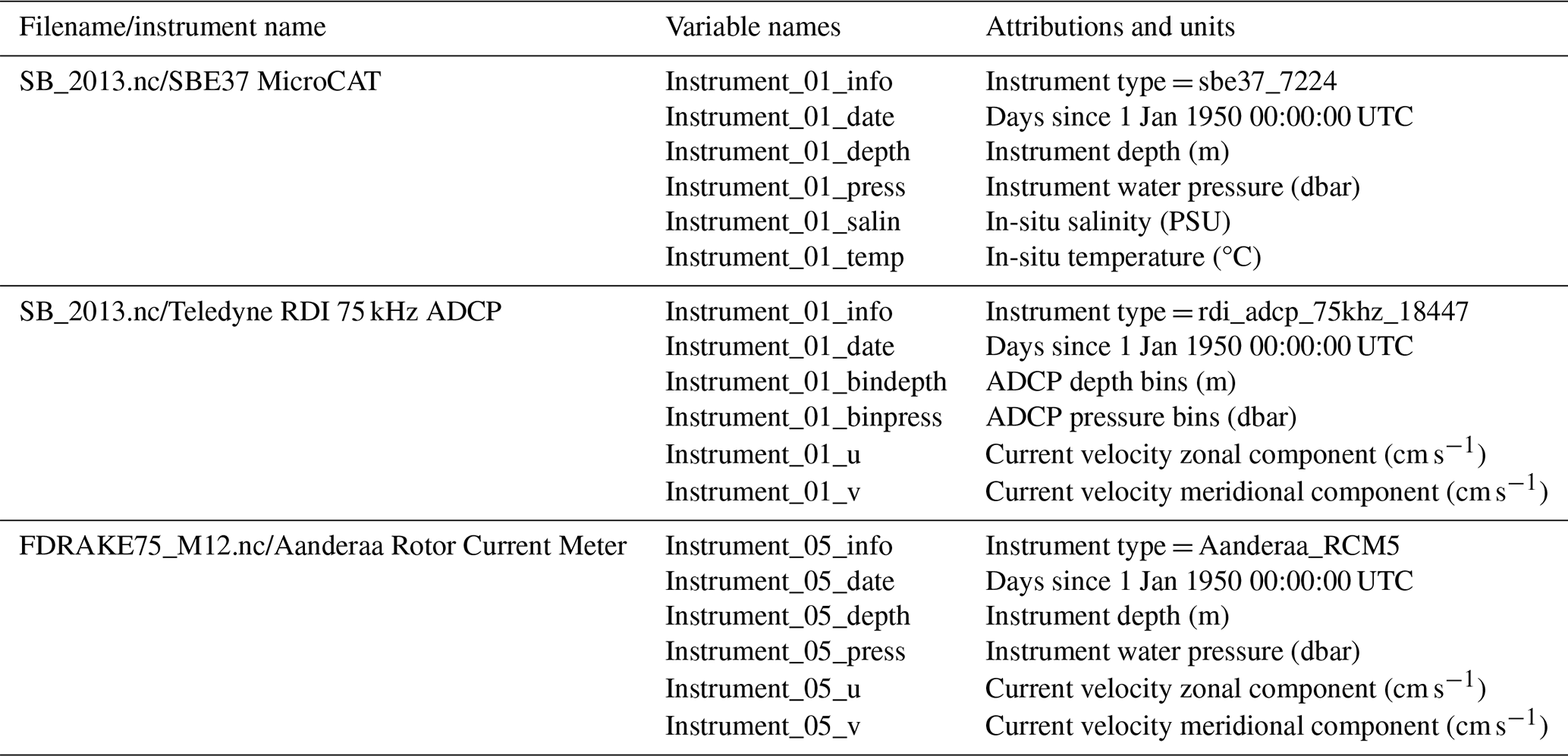
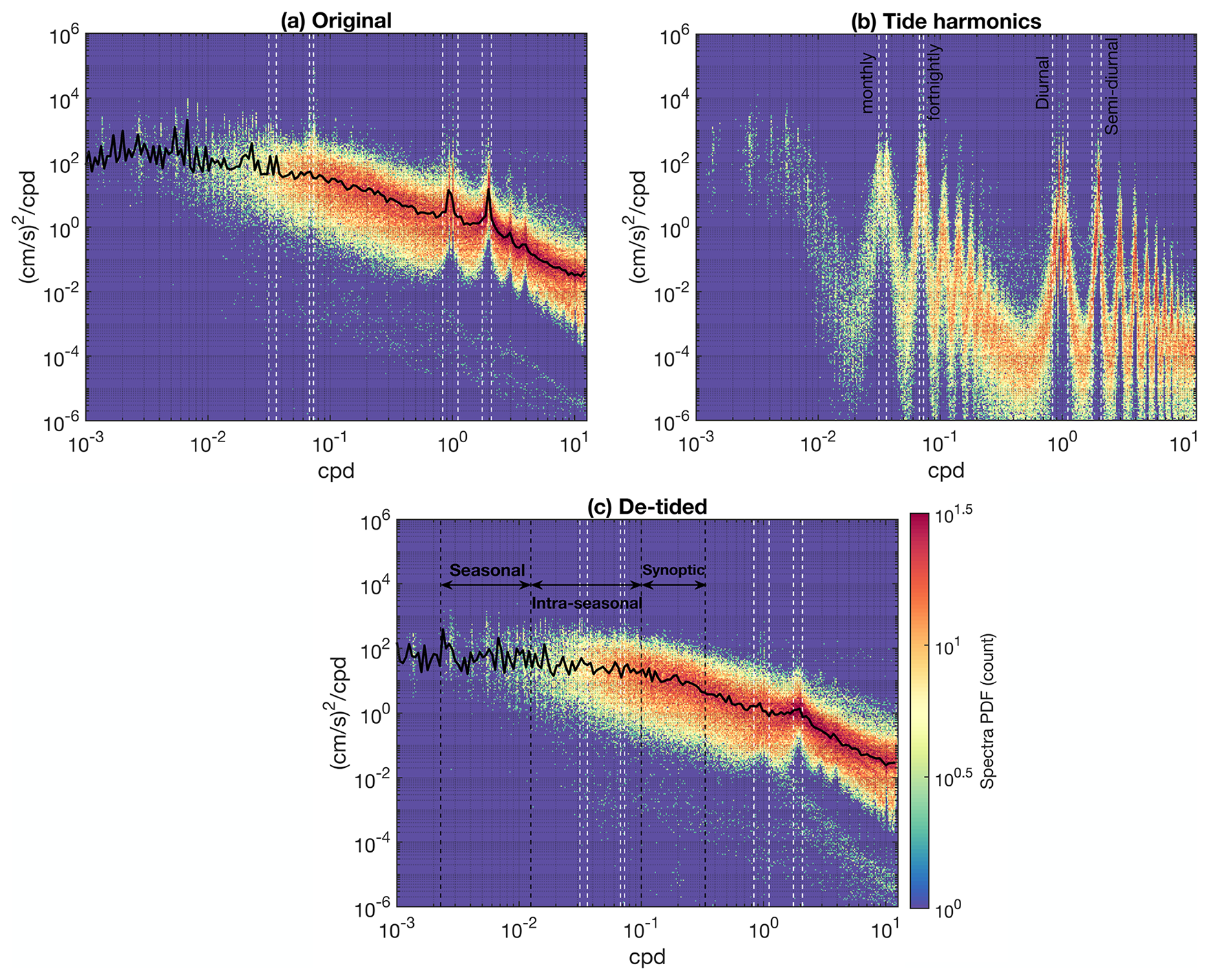
Figure 3 The colour shading shows the spectra probabilistic distribution function (PDF) of all the (a) original velocity time series, (b) the tidal harmonics and (c) de-tided velocity time series. Dashed vertical lines denote the upper and lower frequency bounds for monthly (27.6 to 31.8 d), fortnightly (13.7 to 14.8 d), diurnal (0.9 to 1.2 d) and semi-diurnal (0.48 to 0.57 d) tidal components. Higher/lower values (red/blue) mean that the level of energy is more frequently observed at given frequency across different mooring time series. Black dashed lines in panel (c) show the upper and lower frequency bounds for synoptic (3–10 d), intraseasonal (10–80 d) and seasonal-to-annual (80 d–1.2 years) timescales. Black lines in panel (a) and (c) denote the power density level that is the most frequently counted (i.e. the mode) at each frequency range.

Individual instrument information is available in the variable descriptions, including the name of the instrument and its serial number, if available. For those datasets where the instrument serial numbers were not made available to us, instruments with identical names are differentiated by labelling them numerically in order of the mounted depth along the mooring line. Both acoustic Doppler current meter and current profiler (ADCP) records are included in this compilation, with units of cm s⁻¹, at time *_date (days since 1 January 1950) and depth *_depth (m). Specifically, ADCP data are stored in two-dimensional M×N arrays, M being the number of records, N being the number of vertical bins, and in this case, depth is also two-dimensional. All temperature (°C, IPTS-90) and salinity (Practical Salinity Unit) data stored are in-situ measurements, again using depth and time vectors structured identically to other records in the database.

2.3 Inferred tidal energy and eddy kinetic energy

In the following, we present an initial estimate of the frequency content and spatial distribution of the kinetic energy contained within the compiled records. We isolate the tidal components of the variability from individual records using a multi-linear least square fit to tidal components (UTide, Codiga, 2011), providing us with the fitted tidal harmonics. By removing the fitted tidal harmonics from the original record, “de-tided” time series can be used to reflect the energy associated with non-tidal processes, hereafter referred to as eddy kinetic energy (EKE). In this work, a full list of pre-defined tide constituents (145 in total) was used to compute the complete spectra of tidal signals as the default option in the toolbox to retrieve the first glance of tidal harmonics and de-tided velocity fields. A manual of user-defined parameters and options are discussed in detail by Codiga (2011).

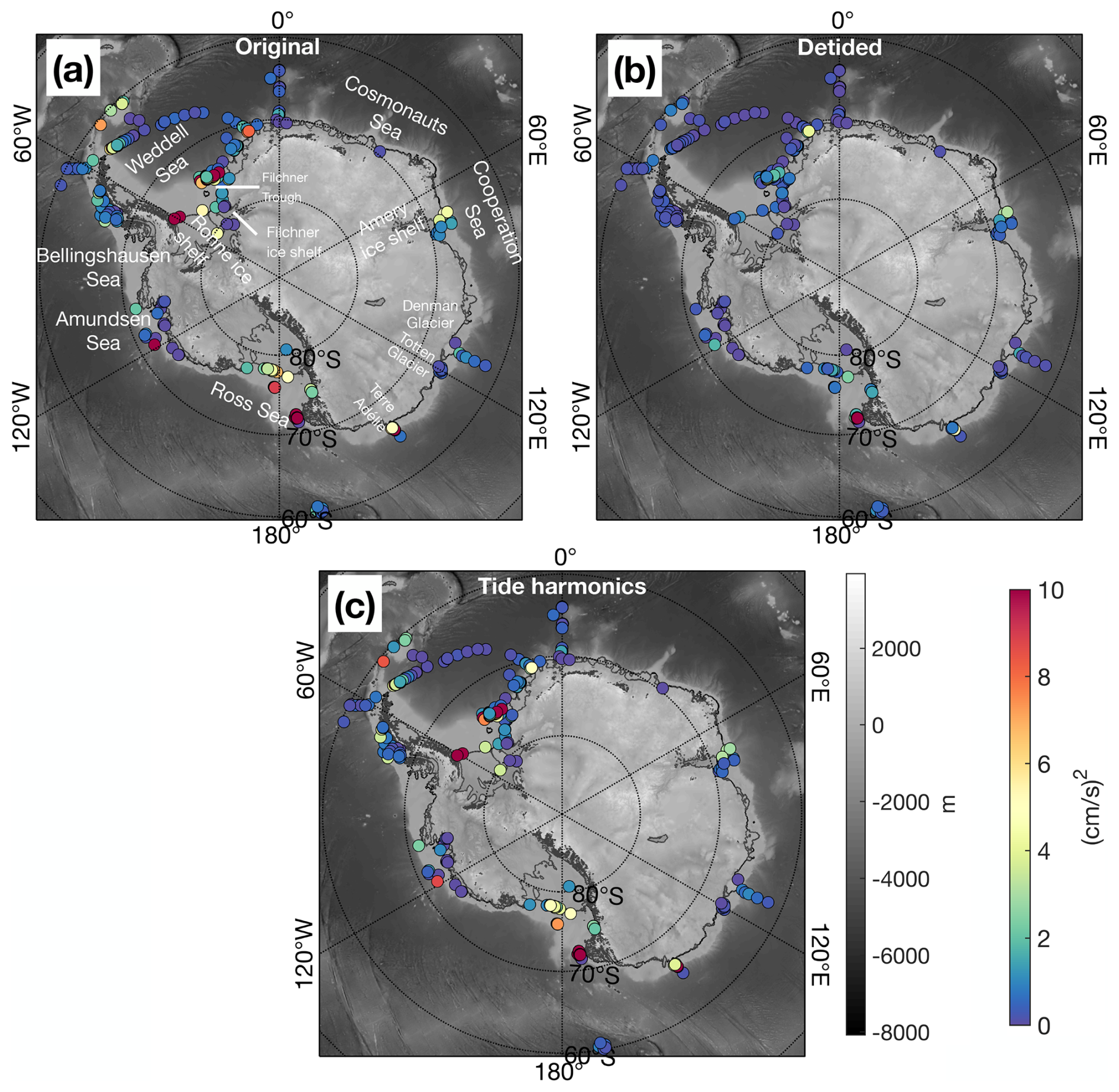
Figure 4 The spatial distribution of the kinetic energy integrated over the diurnal frequency band (0.9 to 1.2 d) using (a) original time series, (b) de-tided time series and (c) fitted tidal harmonics. Grey shading shows the bathymetry, coloured circles showing the magnitude of the kinetic energy integrated over the diurnal frequency band.

Figure 3 shows the probabilistic distribution function (PDF) plot of the current speed spectra integrating all the mooring sites where current meters or ADCPs were deployed. For this exercise, ADCP records are first averaged in the vertical over all recorded bins, giving a single time series per ADCP, from which the spectra are then extracted to be more readily compared with single point current meters. Figure 3a shows the spectra PDF resulting from the original time series. The heat map pattern is predominantly characterised by a classic red spectrum, with pronounced tidal energy peaks at the semi-diurnal (0.48 to 0.57 d), diurnal (0.9 to 1.2 d) and fortnightly (13.7 to 14.8 days) frequency bands. Distinct peaks are also visible for higher and lower frequency tidal harmonics. The spectra PDF of the fitted tidal harmonics is shown in Fig. 3b and highlights the presence of various tidal harmonics and their relatively elevated energy levels. The tide-free or de-tided spectra PDF (Fig. 3c) show a smoother red form, with an overlay of relatively elevated energy peaks around the semi-diurnal frequency range and a smaller, more diffuse energy bump around the synoptic timescales with periods contained between 3 and 10 d.

To provide a view of the spatial distribution of kinetic energy, we further integrate the spectra of all three sets of time series (original, tidal harmonics and de-tided) for each record over a set of frequency ranges, representing the semi-diurnal (0.48 to 0.57 d), diurnal (0.9 to 1.2 d), fortnightly (13.7 to 14.8 d), synoptic (3 to 10 d), intraseasonal (10–80 d) and seasonal-to-annual (80 d to 1.2 years) timescales. An example of the spatial distribution of the kinetic energy before and after the tide removal is shown for the diurnal tidal range in Fig. 4. The original time series (Fig. 4a) in fact contains a range of kinetic energy peaks close to the diurnal periodicity, most of which clearly correspond to the exact tidal harmonics (Fig. 4c), such that the de-tided time series show much lower diurnal peaks. Broadly speaking, most of the ocean kinetic energy at diurnal (Fig. 4b and c), semi-diurnal (Fig. 5a and b), and fortnightly (Fig. 5c and d) periodicity are indeed driven by the tide, and the de-tided energy on these three frequency bands is much lower than the original and tidal harmonics estimations (see also Fig. 3).

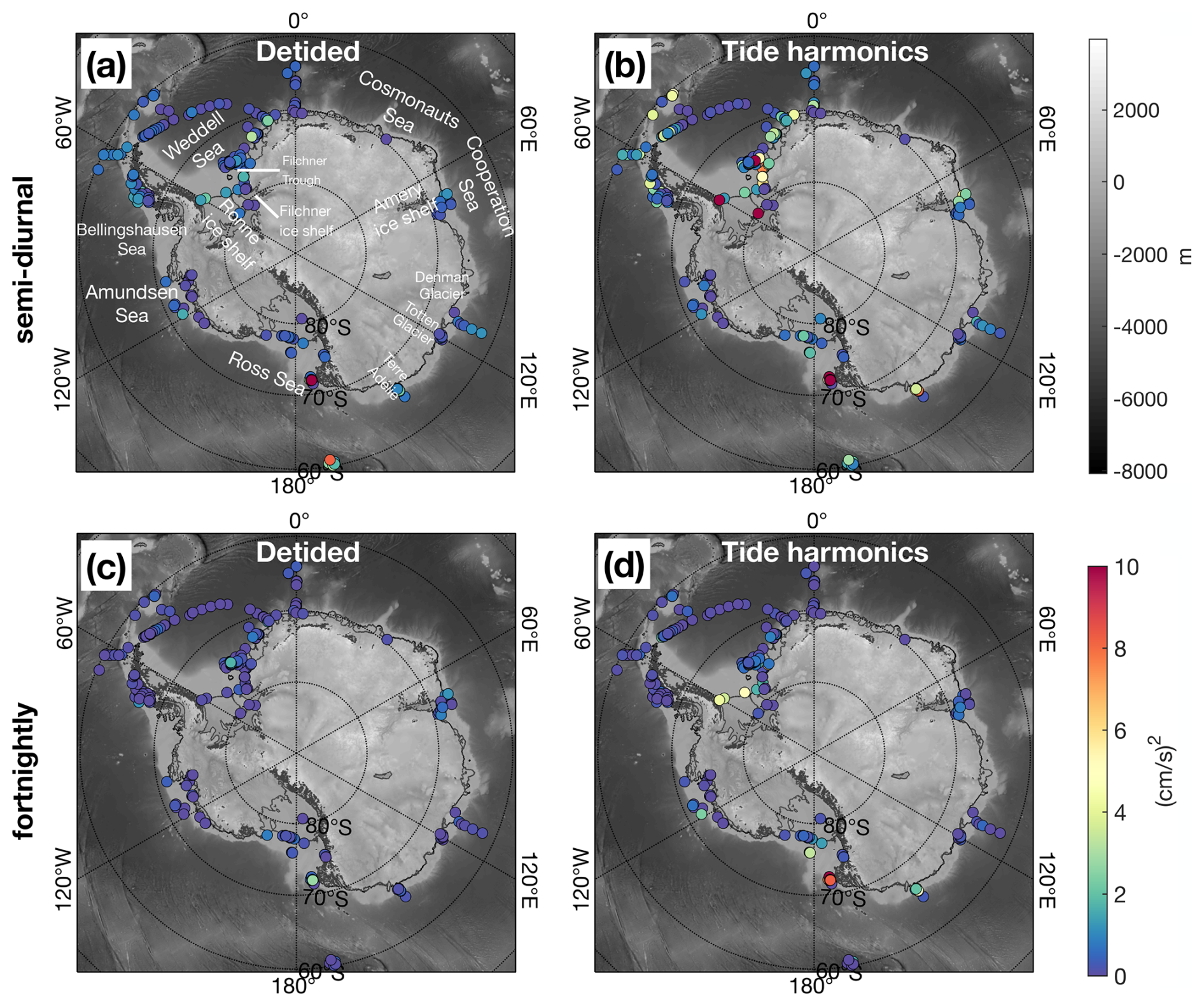
Figure 5 The spatial distribution of (a) de-tided kinetic energy integrated over semi-diurnal periodicity (0.48 to 0.57 d), (b) kinetic energy estimated from fitted tide harmonics over semi-diurnal periodicity. (c, d) Same as (a) and (b) but for fortnightly periodicity (13.7 to 14.8 d). Grey shading shows the bathymetry, coloured circles showing the magnitude of the kinetic energy integrated over the respective frequency bands.

However, we note that some of the de-tided records still retain relatively strong energy levels within the diurnal (Fig. 4b) and semi-diurnal (Fig. 5a) ranges. This property is particularly pronounced in regions where dense shelf water flows out of the Ross Sea, the Cosmonaut Sea (off the Amery Ice Shelf) and the Terre Adélie Sea. The ice front of the Ross and Filchner-Ronne Ice Shelf and the entrance of the Filchner Trough also show elevated levels of diurnal and/or semi-diurnal variability in de-tided time series. The presence of the semi-diurnal to diurnal variability within the de-tided records may result from other sources of variability, e.g. overlapping with the inertial range which is closer to semi-diurnal in polar regions, and/or dispersion of tidal energy around the exact tidal harmonic frequency via mixing processes (e.g., Foster et al., 1987; Whitworth and Orsi, 2006; Padman et al., 2009) or spectral diffusion in more poorly sampled records. Near inertial and tidal motions can be distinguished using rotary spectral analysis, which quantifies kinetic energy as a function of rotational direction. In the Southern Hemisphere, inertial oscillations are consistently anticyclonic, whereas tidal motions may exhibit either cyclonic or anticyclonic rotation (Trasviña et al., 2011). The fact that there is little EKE in the de-tided records at the daily and fortnightly periodicity may indicate a generally low level of spectral diffusion, though this factor is frequency dependent. It also lends support to a hypothesized importance of inertial dynamics as a source of EKE around the semi-diurnal frequency. We note that high kinetic energy (Fig. 5b) is found in mooring sites for de-tided time series where the current meters were instrumented close to the seabed, where the current is arguably more susceptible to turbulence driven by local topography. However, the more detailed analysis required to elucidate the reason for the elevated energy level remaining around tidal frequency ranges within de-tided time series is beyond the scope of this publication.

At lower frequency, EKE can be divided into three bands (Fig. 6), namely synoptic (3 to 10 d), intraseasonal (10 to 80 d) and seasonal-to-annual (80 to 1.2 years) timescales. The synoptic band shows elevated energy levels along most of the Antarctic continental shelf break (Fig. 6a). Inshore, and along glacier fronts, a notable energy distribution pattern emerges – regions corresponding to relatively high depth integrated ocean heat content and associated glacial melt such as the Amundsen and Bellingshausen seas (e.g., Dutrieux et al., 2014; Jenkins et al., 2018; Nakayama et al., 2018) and the Totten (e.g., Rintoul et al., 2016; Gwyther et al., 2018; Silvano et al., 2019) and Denman (e.g., Adusumilli et al., 2020; Miles et al., 2021) glacier fronts all show relatively low synoptic EKE level, in contrast to the higher EKE levels in regions characterised by cold regimes in front of the Ross (e.g., Whitworth and Orsi, 2006; Castagno et al., 2019; Silvano et al., 2020), Filchner-Ronne (e.g., Gordon et al., 2001; Nicholls et al., 2009; Hattermann et al., 2021; Zhou et al., 2023) and Amery ice shelves (e.g., Ohshima et al., 2013). We speculate that this difference is associated with the heightened sensitivity of cold regions to synoptic atmospheric variability through the response of the ocean surface to sea ice formation and stronger katabatic wind events, whilst warmer regions tend to be more stratified, somewhat insulating the lower part of the water column from surface synoptic variability. In addition, the dense water produced through the sea ice formation can also lead to strong pulses of outflow and imprints on the synoptic timescales, leading to heightened EKE levels in cold regimes.

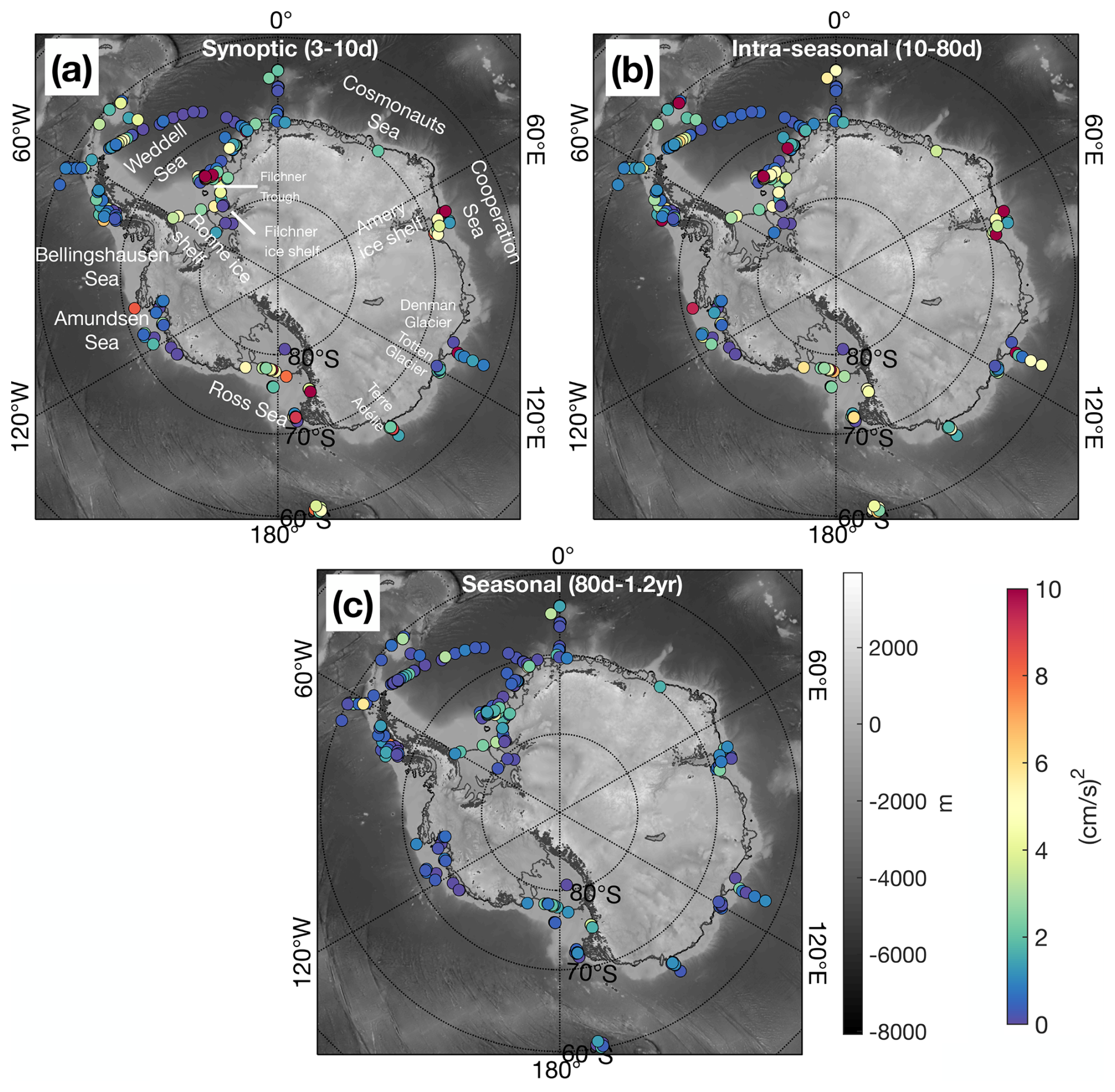
Figure 6 The spatial distribution of the de-tided kinetic energy integrated over (a) synoptic (3 to 10 d), (b) intraseasonal (10 to 80 d), (c) seasonal-to-annual (80 d to 1.2 years) frequency bands. Grey shading shows the bathymetry, coloured circles showing the magnitude of the kinetic energy integrated over the respective frequency bands.

Another source of EKE can be short coastal waves excited by the atmospheric forcing (Chavanne et al., 2010), dense outflows (Jensen et al., 2013) or resulting from local flow instability excited by topographic features (e.g., St-Laurent et al., 2013; Liu et al., 2022). This source of variability, which appears visible in a few bottom pressure records and sea surface height (McKee and Martinson, 2020) would probably apply to a broader range of frequencies, from synoptic to seasonal. Interestingly, the regional pattern of spatial variability in EKE revealed above for synoptic time scales also holds for longer (intraseasonal) time scales (Fig. 6b). A deeper analysis cross correlating atmospheric and ocean variability and applying coastal wave model responses to wind forcing may help to elucidate the processes driving the synoptic-to-intraseasonal EKE. And a more detailed attribution study investigating the processes associated with sea ice formation, dense water production/outflow and the response of ocean currents to the mechanical stirring from the surface stresses is warranted.

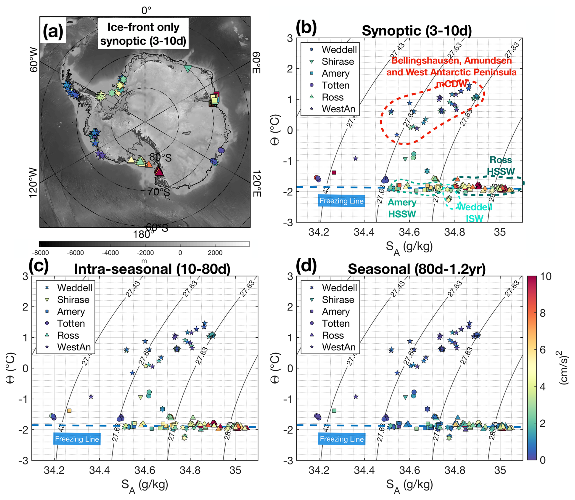
Figure 7 (a) The locations of ice-front moorings coloured by de-tided synoptic scale energy. To avoid overlap, data points from the same mooring sites, but with different sampling depths or time periods, were offset by on average 0.5° in longitude and latitude. Grey shading shows the bathymetry. Panel (b)–(d) shows the EKE magnitude integrated over synoptic, intraseasonal and seasonal-to-annual scales in potential temperature (Θ)-absolute salinity (S_A)-space. The freezing line in the Θ-S_A-space diagram represent the temperature and salinity features associated with surface freezing processes, i.e., the sea ice formation. mCDW locates higher up in the Θ-S_A diagram due to its warm and saline signature while the HSSW falls closer to the freezing line due to its association with sea ice freezing. Depending on the intensity of the sea ice formation rate at different regions, the HSSW can vary in salinity (and density) as seen in the diagram. ISW, the supercooled water mass, falls beneath the surface freezing line as the freezing point is lower at the higher water pressure where ISW is formed (beneath the base of the ice shelf), typically seen in Filchner Sill in the Weddell sector.

Finally, we present the EKE within the seasonal range (Fig. 6c). While the overall EKE level on seasonal timescales is lower than that on synoptic and intraseasonal timescales, the same spatial distribution pattern – whereby EKE levels are enhanced in cold regime shelf seas – still holds. This further highlights the influence of the sea ice thermodynamic and dynamic interactions with the ocean, either through sea ice production and associated deep convection in cold regime shelf seas, and/or modification of the surface stress transmitted by the wind to the ocean via the sea-ice and the downward propagation of this energy to the lower part of the water column (that is more frequently sampled in this database). A deeper analysis is needed to disentangle the roles of each process in each sector, and as a function of time. To further emphasize the regional correlation between local shelf properties and EKE, we sub-selected ice-front moorings within 50 km of the Antarctic ice sheet (Fig. 7a) and plotted EKE at these locations as a function of climatological bottom temperature and salinity (Zhou et al., 2024b), with colour-coded EKE levels displayed in potential temperature-absolute salinity diagrams (Fig. 7b and d). Data points with elevated EKE over synoptic to seasonal scales concentrate near and below the freezing line, confirming that elevated EKE occurs over regions where HSSW are formed (e.g., Filchner-Ronne, Amery and Ross). In contrast, warm ice shelves in West Antarctica (Amundsen, Bellingshausen and the West Antarctic Peninsula sectors) are mostly quiescent on synoptic-to-seasonal timescales after tidal motions are removed.

3 Data availability

The OCEAN ICE mooring compilation is published on SEANOE Data Repository with the doi link, https://doi.org/10.17882/99922 (Zhou et al., 2024a). The data publication contains two files: a compressed file (2.8 GB) including all the mooring time series files in NetCDF format and a spreadsheet containing two tabs – tab 1 lists the mooring file names, locations, starting date, end date and the doi link to the original individual data file; tab 2 lists all the individual instruments in each mooring files, their deployment depth, the observational period, the variables measured and the depth of the seabed of the mooring location.

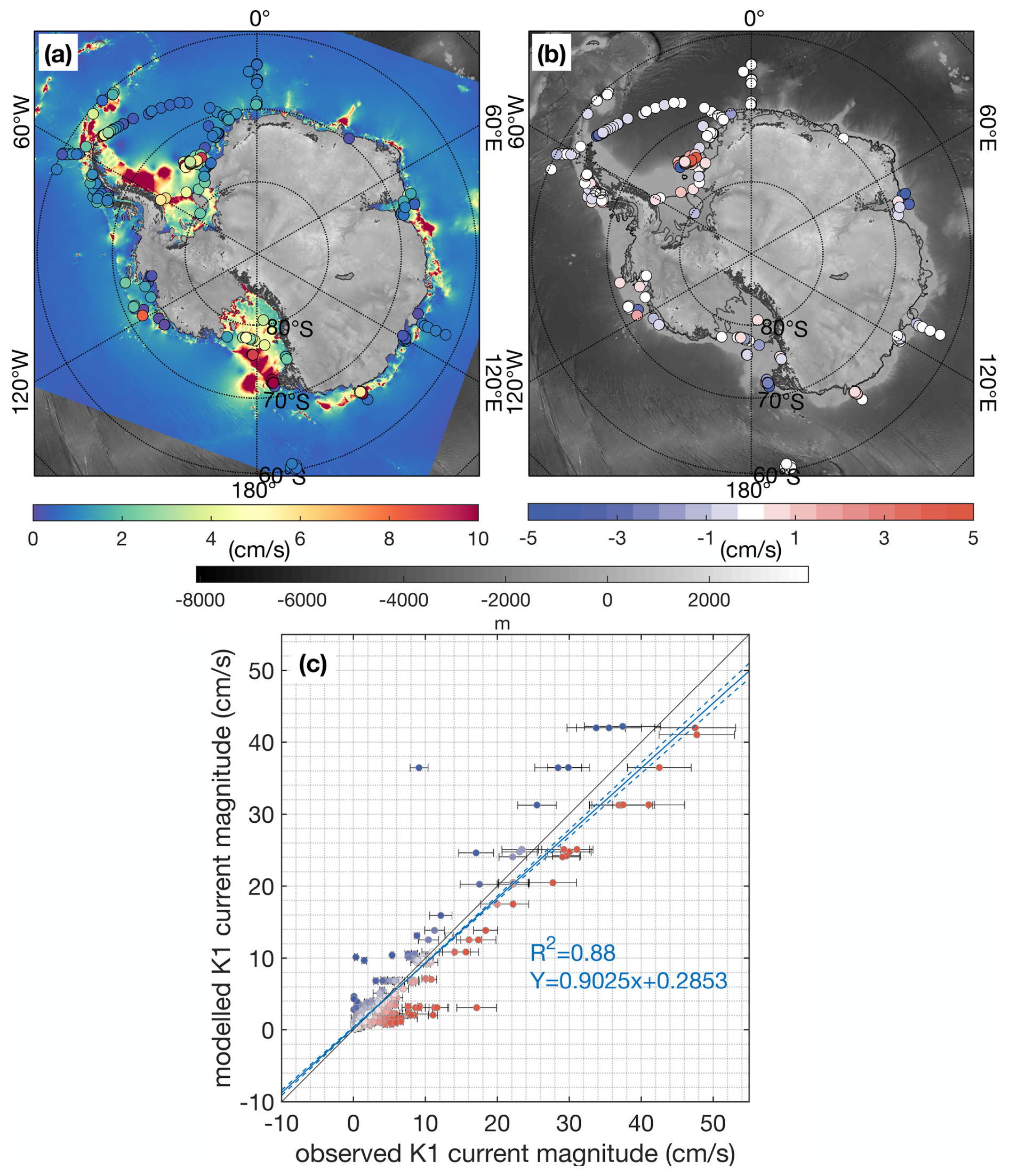
Figure 8 (a) Magnitude of the K1 component of the tidal current (cm s⁻¹) as predicted in CATS2008 (Padman et al., 2002, coloured background) and that fitted with the OCEAN ICE mooring compilation using UTide (overlaid coloured circles). (b) The difference between OCEAN ICE mooring compilation and CATS2008_v2023 model predictions at each mooring location. Red/Blue means moored observations show larger/weaker K1 magnitude compared with the model. Grey shading shows the bathymetry . (c) Scatter plot of OCEAN ICE mooring compilation K1 current magnitude against model prediction. The linear fitting suggests an overall good agreement between two methods, but with significant regional spread. 95 % confidence levels are shown as error bars for the observed K1 magnitude estimated using UTide. Colours showing the same difference in K1 current magnitude as in panel (b).

4 Future work

We have highlighted a few potential avenues for future research above. One additional obvious future element of work remaining at the pan-Antarctic scale is a comparison between observed current tidal harmonics with those predicted by models. Around Antarctica, the most used tide prediction model is the Circum-Antarctic Tide Simulations (CATS, Padman et al., 2002; Padman et al., 2008). This tidal model was recently updated (CATS2008_v2023) with improved representation of coastline, ice shelf grounding line, bathymetry and ice draft (therefore water depth) using the BedMachine Antarctic v3 bathymetry product (Morlighem et al., 2020). It also incorporates an ice flexure model to reflect the tidal deflection near the grounding zone (Howard et al., 2024). Below, we present a brief comparison, focusing solely on the magnitude of the K1 tidal component, which aims at prompting further analysis elsewhere.

A broad agreement between observations and predictions is found over the open ocean, off the continental shelves, where the tidal signals are generally weaker (Fig. 8a and b). Estimates from two methods tend to drift away more significantly over some of the shelf break mooring sites, potentially because of resonant shelf waves at diurnal frequencies (e.g., Semper and Darelius, 2017). Overall, the tidal information extracted from the OCEAN ICE mooring compilation is generally consistent with the CATS2008_v2023 model prediction in K1 periodicity – the model slightly underestimates the K1 current magnitude compared with the observations suggested by the slope of the linear fitting (Fig. 8c). Even with improved BedMachine Antarctica v3 bathymetry information, which does not necessarily provide an accurate bathymetry and ice draft geometry information everywhere (Charrassin et al., 2025), errors in the model predictions can still be sourced from a variety of factors, including incomplete representation of the seabed and ice base geometries, leading to inaccurate water-column thickness. These factors are expected to be specifically significant underneath ice shelves and over the continental shelves where sea ice historically precluded detailed observations of the geometry (Padman et al., 2002). The assumption of the barotropicity in tidal currents by CATS2008_v2023 tide model may also become problematic in regions featuring complex topographies or in regions with distinct vertical stratification, where internal tides with amplitude and phase varying in depth have been documented in Antarctic continental shelf and Southern Ocean settings (e.g., Makinson, 2002; Makinson et al., 2006; Heywood et al., 2007). A more detailed analysis, comparing predictions to observations at other frequencies, or scrutinising the baroclinicity of tidal flows at available observation sites, would help refine the prediction model. Given the importance of tides for numerous processes in Antarctic shelf seas, from ice flexure and impacts on grounding zone positions (e.g. Wallis et al., 2024), migration (Rignot et al., 2024), and ice-ocean interactions (Gadi et al., 2023), improving predictions would be a very useful endeavour. We hope the OCEAN ICE compilation presented here will provide a continuously growing backbone for regional and circum-Antarctic analyses in years to come.