Observational ozone datasets over the global oceans and polar regions (version 2024)

Studying tropospheric ozone over the remote areas of the planet, such as the open oceans and the polar regions, is crucial to understand the role of ozone as a global climate forcer and regulator of atmospheric oxidative capacity. A focus on the pristine oceanic and polar regions complements the available land-based datasets and provides insights into key photochemical and depositional loss processes that control the concentrations and spatiotemporal variability in ozone as well as the physicochemical mechanisms driving these patterns. However, an assessment of the role of ozone over the oceanic and polar regions has been hampered by a lack of comprehensive observational datasets. Here, we present the first comprehensive collection of ozone data over the oceans and the polar regions. The overall dataset consists of 77 ship cruises/buoy-based observations and 48 aircraft-based campaigns. The dataset, consisting of more than 630 000 independent ozone measurement data points covering the period from 1977 to 2022 and an altitude range from the surface to 5000 m (with a focus on the lowest 2000 m), allows systematic analyses of the spatiotemporal distribution and long-term trends over the 11 defined ocean/polar regions. The datasets from ships, buoys, and aircraft are complemented by ozonesonde data from 29 launch sites or field campaigns and by 21 non-polar and 17 polar ground-based station datasets. The datasets contain information on how long the observed air masses were isolated from land, as estimated by backward trajectories from the individual observation points. To extract observations representative of oceanic conditions, we recommend using a subset of the data with an isolation time of 72 h or longer, from the analysis with coincident radon observations. These filtered oceanic and polar data showed typically flat diurnal cycles at high latitudes, whereas daytime decreases in ozone (11 %–16 %) were observed at lower latitudes. The ship/buoy- and aircraft-based datasets presented here will supplement the land-based ones in the TOAR-II (Tropospheric Ozone Assessment Report Phase II) database to provide a fully global assessment of tropospheric ozone. The described dataset is available at https://doi.org/10.17596/0004044 (Kanaya et al., 2025).

1 Introduction

As a short-lived species with an estimated lifetime of 25.5±2.2 d (Griffiths et al., 2021; Szopa et al., 2021), both global/hemispheric and regional/local aspects need to be emphasized in the assessment of tropospheric ozone. While the spatiotemporal variation over land is primarily important for assessing vegetation and health impacts, its behavior over the oceans is critical when assessing its climate impact as the third most important greenhouse gas (Forster et al., 2021). The role of ozone in maintaining the global oxidative capacity of the atmosphere through the production of the OH radical also requires understanding on a global scale. The overall budget of tropospheric ozone is dominated by the photochemical production and loss terms, estimated at 4500–5000 and 3900–4500 Tg yr⁻¹, respectively, rather than by the stratosphere–troposphere exchange (270–540 Tg yr⁻¹) or surface deposition (800–1000 Tg yr⁻¹) for decades around 2000 or 2010 (Griffiths et al., 2021; Young et al., 2018). The net ozone production mainly occurs over regions with NO_x pollution and depends on the abundance of volatile organic compounds (VOCs). By contrast, the net loss conditions, which are driven by OH/HO₂ radical chemistry in a low-NO_x environment and potentially also by understudied halogen chemistry, occur mostly over remote regions, including over the oceans (Galbally et al., 2000; Monks et al., 1998; Stone et al., 2018; Read et al., 2008; Dickerson et al., 1999; Boylan et al., 2015; Saiz-Lopez and von Glasow, 2012; Simpson et al., 2015). Another important loss term is from dry deposition on the ocean surface, which depends on the chemical composition of the surface seawater and its physical conditions (Helmig et al., 2012; Hardacre et al., 2015; Ganzeveld et al., 2009; Pound et al., 2020; Sarwar et al., 2016; Luhar et al., 2018; Barten et al., 2023; Chiu et al., 2024) and which has not been fully characterized. Therefore, there is a special need to study the ozone concentration levels and spatiotemporal variations as well as the underlying mechanisms that control ozone levels over the oceans. However, observational data of ozone over oceanic regions are much less abundant than those over the land, preventing a full assessment. TOAR (Tropospheric Ozone Assessment Report) is an IGAC (International Global Atmospheric Chemistry project)-sponsored activity which aims to collect ozone observations in the troposphere. At the time of TOAR-I (Schultz et al., 2017), oceanic data were collected only from island-based surface monitoring observations and ozonesondes, with some satellite-based information, but the oceanic regions remained devoid of data.

The polar regions are other pristine areas, with episodic ozone destruction in the polar sunrise season (Simpson et al., 2007). During the International Polar Year 2007–2008, extensive studies on ozone were conducted and published and published in the POLARCAT (Polar Study using Aircraft, Remote Sensing, Surface Measurements and Models, of Climate, Chemistry, Aerosols, and Transport) special issue (ACP, 2015). An assessment report on short-lived climate forcers from the Arctic Council's Arctic Monitoring and Assessment Programme (AMAP, 2021) and synthesis papers (Whaley et al., 2023; Law et al., 2023) have recently been produced, but comprehensive studies based on multi-platform observations are still lacking.

To improve the situation, a working group on ozone over the oceans and the polar regions (Oceans working group) has been formed within the TOAR-II activity to provide a comprehensive dataset, especially with ship-, buoy-, and aircraft-based observations over the oceans, to allow a first assessment over the entire ocean area and polar regions. In the past, studies on ozone over the oceans were conducted using ship-based/aircraft-based ozone observations, but they were mostly based on observations from a single campaign/series of related campaigns (e.g., Dickerson et al., 1999; Bourgeois et al., 2020) or, at best, from a collection of observations from a single nation/project (e.g., Lelieveld et al., 2004; Kanaya et al., 2019); here we aim to collect data from multiple nations, research groups, and campaigns to achieve a better global coverage, using the IGAC framework as a global research network (GRN) of Future Earth, on which the TOAR activity is based. The resulting five datasets include observations from ships/buoys, aircraft, ozonesondes, ground-based coastal/island sites, and polar stations. This data paper primarily describes two of these datasets, which consist of 77 ship- or buoy-based observations and 48 aircraft observations over the global oceans and polar regions covering a period between 1977 and 2022. The altitude range covered by the data is from the surface to 5000 m, with a focus on the lowest 2000 m, as a major interest of the working group lies within the atmospheric boundary layer, where the interfacial interactions of the atmosphere with the ocean and snow/ice surfaces (even including biogeochemical processes), as well as the photochemistry, are of particular relevance. A third dataset contains ocean and polar ozonesonde data, mostly obtained from coastal/island sonde launching sites. The ozonesonde data were mainly provided by the HEGIFTOM (Harmonization and Evaluation of Ground-based Instruments for Free-Tropospheric Ozone Measurements) Focus Working Group of the TOAR-II activity and, therefore, include their data homogenization procedure (Van Malderen et al., 2025), but they were further processed by the Oceans working group here. These three datasets are complemented by two datasets containing ground-based data from coastal/island sites and from polar stations, selected from the TOAR-II database (Schröder et al., 2024) with some additional field campaign sites. Satellite data are not included in this study because they are discussed elsewhere in the TOAR-II special issue (Gaudel et al., 2024; Pope et al., 2023) and because it is still difficult to resolve the commonly low ozone levels in the boundary layer over the oceans from satellite observations.

The result of this work enables integrated studies of the long-term and/or seasonal trends from ship-based observations and established coastal-site observations in the same region, for example, at Cabo Verde, Kennaook/Cape Grim, Mace Head, and Trinidad Head (e.g., Parrish et al., 2009). To be suited for the ocean-focused studies, all five datasets are complemented with information on how many hours each observed air mass was separated from land, derived from backward trajectories. Note that a full assessment of tropospheric ozone in the remote regions (oceans and polar) using these datasets will be published separately (Sommariva et al., 2025) as part of the TOAR-II series of assessment papers; here, we focus on the data description, including its preparation and harmonization.

2 Data description

The overall geographical distribution of the collected ship/buoy data, aircraft-based data (up to 5000 m but considering 0–2000 m altitude as a key part for the study of the boundary layer), and selected ozonesonde/surface observation sites is shown in Fig. 1. The following subsections describe each dataset in detail. The data are divided into 11 regions (2 polar and 9 oceanic). Following the recommendation of the TOAR-II Steering Committee (TOAR-II Steering Committee, 2023), the regions are broadly defined as follows: polar (60–90° N and 90–60° S), midlatitude (20–60° N and 60–20° S), and tropical (20° S–20° N). The boundaries are adjusted by 4° or less to take into account geography or the position of the land masses (Fig. 1). The Pacific sector (from 100–115° E to 100–69° W, across the International Date Line) is subdivided into northern (R1; 22–63° N), tropical (R2; 20° S–22° N), and southern (R3; 60–20° S) regions. The Indian Ocean (from 20–34° E to 100–115° E) is divided into tropical (R4; 20° S–31° N) and southern (R5; 60–20° S) regions. The eastern part of the Mediterranean Sea and the Black Sea (15–55° E, 31–59° N) are given a code R6, but we did not collect data from these areas because continental influences were generally unavoidable. The Atlantic sector (from 100–69° W to 15–20° E) is divided into northern (R7; from 16–23 to 62° N), tropical (R8; 20° S–23° N, including the Caribbean), and southern (R9; 60–20° S) regions. The Arctic region (R10) is defined as north of 59–63° N (depending on the longitude) and the Antarctic region (R11) as south of 60° S.

Figure 1 Locations of ozonesonde and coastal/polar ground observations (a). Overall ship/buoy ozone data (b) and airborne ozone data with altitudes < 2000 m (c) after filtering for LCL ≥ 72 h. Ozone levels above 60 ppb are omitted for clarity.

2.1 Ship/buoy dataset

A total of 208 291 hourly averaged ozone concentration data were collected from 62 ship cruises (or aggregated cruises/legs) and from 15 buoy operations and archived in the file toar2_oceans_ship_buoy_data_250203.csv, covering the 1977–2022 period (Table 1, Fig. 1). The data come from research groups in the USA, Japan, Australia, Germany, France, Switzerland, Spain, India, and the Republic of Korea. The instruments used are mainly research-grade ozone monitors based on UV absorption, with the exception of the DWD-MPI (Deutscher Wetterdienst – Max Planck Institute) dataset before 1996 which employed a wet chemical instrument using the potassium iodide (KI) method. The ship's exhaust plume could affect all of the cruise observations, depending on the relative wind directions with respect to the ship's funnel and the inlet position of the gas sampling tube. A fast-response ozone monitor could easily detect such cases of pollution, as NO in the exhaust titrates the atmospheric ozone quickly. The buoy measurements do not have the risk of a plume effect; therefore, their hourly averages were constructed from the original 10 s raw data without filtering to preserve the real ozone reduction episodes over the Arctic region.

The ship datasets were processed as follows. First, minute data below the hourly mean minus 1σ were removed. Following this, hourly averages were recalculated. The hourly data were removed if the variability in the valid minute data was greater than 10 % of the hourly mean. This two-step filtering procedure is similar to Kanaya et al. (2019) and was found to be suitable to remove the ship's influence in different cruise datasets. Figure S1 in the Supplement shows a case of flagging and data removal from the time series of the R/V Hakuho Maru cruise KH18-6. Filtering was applied to cruises for which 1 min resolution data were available, i.e., R/V Mirai cruises during 2012–2021 (MR 12–21), Hakuho Maru KH-18-6, NAAMES1–4, ATOMIC, DYNAMO, WACS, VOCALS, NEAQS 2002, NEAQS 2004, TEXAQS 2006, ICEALOT, CalNex 2010, DRAKE2009, IN MAP-IO (SWINGS 2021, OP1 TAAF 2021, SCRATCH 2021, OP2 TAAF 2021, MAYOBS 2021, OP3 TAAF 2021, and OP4 TAAF 2021; http://173.249.47.189/new_mapio_web/home/, last access: 6 September 2025), Ka'imimoana, 17v01-05, 18v01-06, 08, 19v01-03, IIOE2, SOE9, and SOE11. The original data from MAGE92, RITS93, RITS94, ACE1, AEROSOLS99-INDOEX, and ACE-Asia were on a 30 min basis and were averaged to an hourly resolution. The original hourly data from Malaspina, SAGA3, DWD-MPI, YES-AQ, and MOSAiC were used as they were provided. We assumed that basic quality control had been performed (e.g., see Angot et al., 2022, for the MOSAiC dataset). The DWD-MPI data are a large compilation of 51 cruises with different research vessels (Meteor, Polarstern, Walther Herwig, Anton Dohrn, Ymer, and Academie Fedorov) collected by Deutscher Wetterdienst (DWD) in the 1977–1996 period, 27 cruises with the container ship Berlin Express collected by Max Planck Institute (MPI) in the 1995–2002 period, and one Meteor cruise conducted by MPI in 2002, with a clear note that the data have been screened for local influences of the research vessel itself and of nearby passing ships and that data in and near harbors and in channels have been removed.

Some cruises included additional observations of pollution tracers, i.e., CO, NO, NO₂, and condensation nuclei (CN) with diameters larger than 11–13 nm, and these data are archived together with ozone (see Table 1 and Table S1 in the Supplement for the observation methods and uncertainties). However, the tracer observations did not cover the entire dataset and, therefore, could not be used uniformly for further systematic screening of air masses influenced by pollution arising from nearby land (even if present). It is an essential requirement of oceanic ozone studies to be able to distinguish between air masses representing the remote ocean and those influenced by pollution from nearby land. Therefore, we calculated backward trajectories for each hourly dataset to add information on the “last contact with land” (LCL, in the unit of hours ago), as a semi-quantitative index indicating how long the air masses were isolated from a land region with potential pollution before the observations. The land mask data from NASA (NASA, 2019) with a resolution of 0.25° were used. The high-latitude regions (65–90° N or 90–60° S) were not considered to be “land”, and the land mask was assumed only up to an altitude of 2500 m, as the pollution effect from land would be minimal at higher altitudes. Exceptions may include lifted plumes, such as those from biomass burning. The 2500 m threshold is tentative in an attempt to yield a criterion that is meaningful for the entire globe. It may be revisited after detailed analysis in the assessment. Backward trajectories were computed with the HYSPLIT version 4 model (Draxler and Rolph, 2013) using 6-hourly GDAS1 (1×1°) meteorological fields after December 2004 or using 6-hourly NCEP/NCAR Reanalysis product (RP{YEAR}{MONTH}.bgl) files with a 2.5° resolution for the earlier period. Harris et al. (2005) studied the uncertainty in the trajectories using the NCEP/NCAR Reanalysis product. The starting altitude for ship/buoy observations was set to 500 m and the duration to 120 h. The first point of land contact was marked to provide the LCL information. An LCL value of 120 h was assigned to the air masses if no land contact occurred for the entire period.

We defined a criterion of LCL ≥ 72 h (hereafter referred to as LCL72) to identify marine air masses that have been minimally influenced by land. Figure 2 shows examples of the backward trajectories calculated for the MR19-03C cruise between Japan and the Arctic and for the RITS94 cruise from North to South America, respectively. The light-blue and purple lines represent trajectories for marine and land-influenced air mass cases, respectively. The red lines indicate the cases in which the observed ozone mixing ratio was greater than 50 ppb (polluted).

Table 1 List of cruise/buoy data contained in the ship/buoy data file.

Note that NA represents “not available”.

The LCL72 criterion was evaluated using observed radon concentrations from ACE-1 (Whittlestone et al., 1998), ACE-Asia, ATOMIC, ICEALOT, NAAMES1–4, and WACS shipborne observations as a tracer of land contact (Fig. 3). Radon, emitted from land and lost with a half-life of 3.8 d (Zhang et al., 2021), is suitable for testing the performance of 120 h trajectories and then removing the cases affected by fresh pollution. The median and third-quartile radon levels are diminished by almost two-thirds when LCL increases from 10 to 80 h, with a clear drop occurring between 60 and 80 h since the last contact with land. This provides the basis for a 72 h LCL threshold for identifying marine air masses with little or no influence from land.

Although the discrimination between oceanic and land-influenced air masses is imperfect, largely due to the uncertainties in the trajectory calculations, the agreement between the LCL72 and the radon < 1000 mBq m⁻³ criteria (during the campaigns for which this parameter was available) suggests that it is reasonable to apply the LCL72 flag to all of the data treated in this study over the global oceans as the first filter against land influences. In subsequent studies on this oceanic ozone dataset, other filters of land influence can be developed and used to meet the requirements of the type of analysis being undertaken. For example, a more stringent criterion (radon < 100 mBq m⁻³) was used to select baseline data at the Kennaook/Cape Grim station (Chambers et al., 2018). The data that met the LCL72 criterion covered 161 037 h (77 % of the original dataset). Note that the data with a LCL of less than 72 h are kept in the data file, as they may be useful for other purposes.

2.2 Aircraft data

Table 2 lists the 48 airborne campaigns included in the toar2_oceans_airborne_data_5000m_250203.csv dataset. The land mask mentioned in Sect. 2.1 was used to extract the airborne observations over the oceans. The high-latitude data (65–90° N or 90–60° S) were not masked and were used directly. The original merge-type data files from aircraft observations had different time resolutions, from <10 to 90 s; particularly for old missions, only a coarse time resolution was available. Considering the temporal coverage and taking advantage of the relatively high temporal resolution of the more recent data, a variable temporal resolution in the range of 10–90 s was used. For campaigns where data with a higher temporal resolution (e.g., 1 Hz) were available, e.g., from FAAM measurements, the data were averaged over 10 s. A total of 424 005 and 252 086 data records for the respective altitudes of < 5000 and <2000 m are included in the dataset, covering a period from 1987 to 2020. The data originated from the USA, the UK, and Germany/Canada, and they covered almost all global regions except for the R4 region (tropical Indian Ocean). Data for R5 (southern Indian Ocean) were sparse: only 62 points from the TRACE-A mission. The instruments used for the measurements of ozone are generally based on fast-response instruments, e.g., high-sensitivity chemiluminescence or UV absorption. Additional data on observations of pollutant tracers, i.e., CO, NO, and NO₂, were archived together (Table S2). The backward trajectories were applied to each measurement point, similar to the ship/buoy-based data, with the starting altitude set to the GPS altitude of the aircraft or to 500 m when it was lower. The proportions of the data meeting the LCL72 criterion were 74 % and 63 % for the <5000 and <2000 m cases, respectively. This was partly affected by the assumed top altitude boundary of “land” at 2500 m. The bottom panel of Fig. 1 shows the data meeting the LCL72 criterion at an altitude < 2000 m.

2.3 Ozonesonde data

A total of 29 selected ozonesonde launch sites/campaigns are included in the toar2_oceans_ozonesondedata_250203.csv dataset. The sites are listed in Table S3 and shown in Fig. 1. There are no data for regions R4 (Indian Ocean) and R9 (South Atlantic). As the availability of geopotential height information was considered a high priority in the creation of the dataset, data from earlier dates when this parameter was not available (e.g., Alert before 2000) were not included. Their inclusion could be a future task. The ozone mixing ratio was calculated from the atmospheric pressure and the ozone partial pressure data. To reduce the data volume, one data point every 200 m (data closest to the top of each layer, e.g., near 200 or 400 m) was extracted up to a 5000 m altitude. The ($\mathrm{1}/e$) ozone sensor response time (∼30 s) gives the ozonesonde a vertical resolution of about 150 m for a typical balloon ascent rate (Van Malderen et al., 2025). Most of the sites (24 out of 29) were taken from the homogenized HEGIFTOM dataset (Van Malderen et al., 2025) to ensure data quality. The selected launch sites are on islands or close to the coast. The other five data sources are from island and shipboard campaigns in the tropical Pacific (Gómez Martín et al., 2016; Shiotani et al., 2002; Fujiwara et al., 2003), with the addition of three datasets in R11 (Antarctic region) from the World Ozone and Ultraviolet Radiation Data Centre (WOUDC) ozonesonde database to improve the coverage. The data are all from electrochemical concentration cell (ECC)-type ozonesondes. In total, 666 470 and 254 276 data points below respective altitudes of 5000 and 2000 m were collected.

Figure 2 Backward trajectories (120 h long) for observations with oceanic (light blue) and apparently land-influenced (purple) conditions, as assessed with the LCL72 criterion during (a) the MR19-03C observations from 29 September to 10 November 2019 and (b) the RITS94 observations from 23 November 1993 to 6 January 1994. The red lines indicate cases in which the observed ozone mixing ratio is greater than 50 ppb.

Figure 3 Decrease in radon concentrations with last contact with land from backward-trajectory analysis. ACE-1, ACE-Asia, ATOMIC, ICEALOT, NAAMES1-4, and WACS data were used in combination. Radon data were from NOAA PMEL. The dotted blue line indicates the adopted LCL72 criterion. Boxes and whiskers represent the 10th, 25th, 50th, 75th, and 90th percentiles.

Table 2 List of aircraft-based campaign data contained in the aircraft dataset.

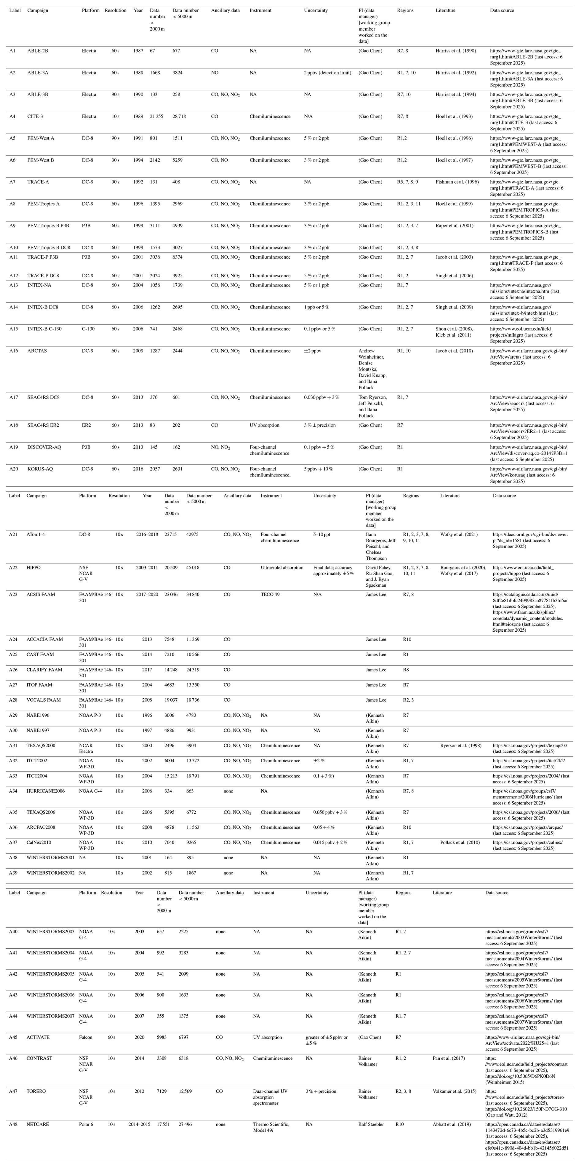
Note that NA represents “not available”.

Backward-trajectory calculations were only performed for selected heights (500, 1000, 1500, 2000, 3000, 4000, and 5000 m) to reduce the computational cost. The LCL information relative to the closest of the height points was used. The proportions of the data meeting the LCL72 criterion were 80 % and 67 % for the full dataset (<5000 m altitude) and for the <2000 m data subset, respectively. As the launch site is usually on land, the latitude/longitude information from the backward trajectories at 0 and 1 h prior to launch was not included in the LCL calculation. Therefore, the potential influence of local air pollution in the vicinity of the launch site needs to be considered when using these data. For a further characterization of air masses and screening, wind direction sector information (Table S3), constructed from the coordinates from the backward-trajectory files at 0 and 1 h before launch, was added to the dataset.

2.4 Non-polar coastal site data

The list of 21 non-polar coastal sites included in the toar2_oceans_coastalsites_250203.csv file is shown in Table S4, and their locations are given in Fig. 1: 16 sites are from the TOAR-II database (Schröder et al., 2024), 2 are from field campaigns, 2 are from the EANET monitoring network, and 1 is from CSIRO. The sites were selected on the basis of the availability of high-quality data over long periods (typically >10 years) and for the global coverage. However, no sites matching these criteria could be found for regions R4 and R5 (Indian Ocean). The Kennaook/Cape Grim dataset available on the TOAR-II database was not used; rather, another dataset provided by CSIRO was employed. The latter was an updated version, extended through to the end of 2020, with the years 1982–2017 inclusive being fully QA/QC data on the WMO GAW/BiPM scale. The 2018–2020 period was in the final stages of QA/QC, and the fully finalized dataset has subsequently been published on EBAS (EBAS, 2025). Further information on the instruments and uncertainties for each site can be found in the TOAR-II database. Obviously, the incorrect data (i.e., zero or negative values) have been removed, resulting in a total of 3 650 267 hourly observations being included. The LCL information based on the backward trajectories is included. To reduce the computational cost, only 6 hourly calculations were performed, and the result at the closest data timestamp was used. It should be noted that the risk of the influence from local air pollution is similar to that of the ozonesonde dataset. Data from Trinidad Head can be screened using the local wind direction information (as shown in Table S3).

2.5 Polar site data

The list of 17 polar coastal sites included in the toar2_oceans_polarsites_250203.csv file is shown in Table S5 and Fig. 1. Except for Alert and Belgrano stations, where the data came from the Canadian data site and from the National Institute for Aerospace Technology (INTA), respectively, the 15 datasets are from the TOAR-II database. A total of 3 362 716 hourly observations were included. Similarly to the case of the non-polar coastal sites, the LCL information based on the backward trajectories is included. To save computational cost, only 6-hourly trajectory calculations were performed, and the result at the closest data timestamp was used.

3 Data overview

In this section, some basic data analysis and descriptive statistics of the collected datasets are described, for informational purposes. Detailed discussion of the spatiotemporal distribution of tropospheric ozone and its trends over the oceans and polar regions will be presented in the assessment paper (Sommariva et al., 2025).

3.1 Latitudinal, longitudinal, and vertical transects

Figure 4 shows the latitudinal and longitudinal cross sections of the ship/buoy data after application of the LCL72 filter. The data are grouped into 10° latitudinal and 20° longitudinal bins. The median values in the Southern Hemisphere are in the range of 15.2–19.1 ppb, while those in the Northern Hemisphere are in the range of 20.5–34.0 ppb. As expected, a maximum median value was found between 25 and 55° N, where the ozone is photochemically produced from precursors anthropogenically emitted over the continents and transported over long distances to the open oceans (Fig. 1; see also Kanaya et al., 2019). The longitudinal distribution has less variability, with median values in a narrow range of ca. 20–30 ppb. The high episodes (higher than the 75th percentile) are evident from 35 to 45° N and from 120 to 140° E, suggesting that the effects of Asian pollution remain in the dataset, consistent with the discussion regarding the LCL72 filter.

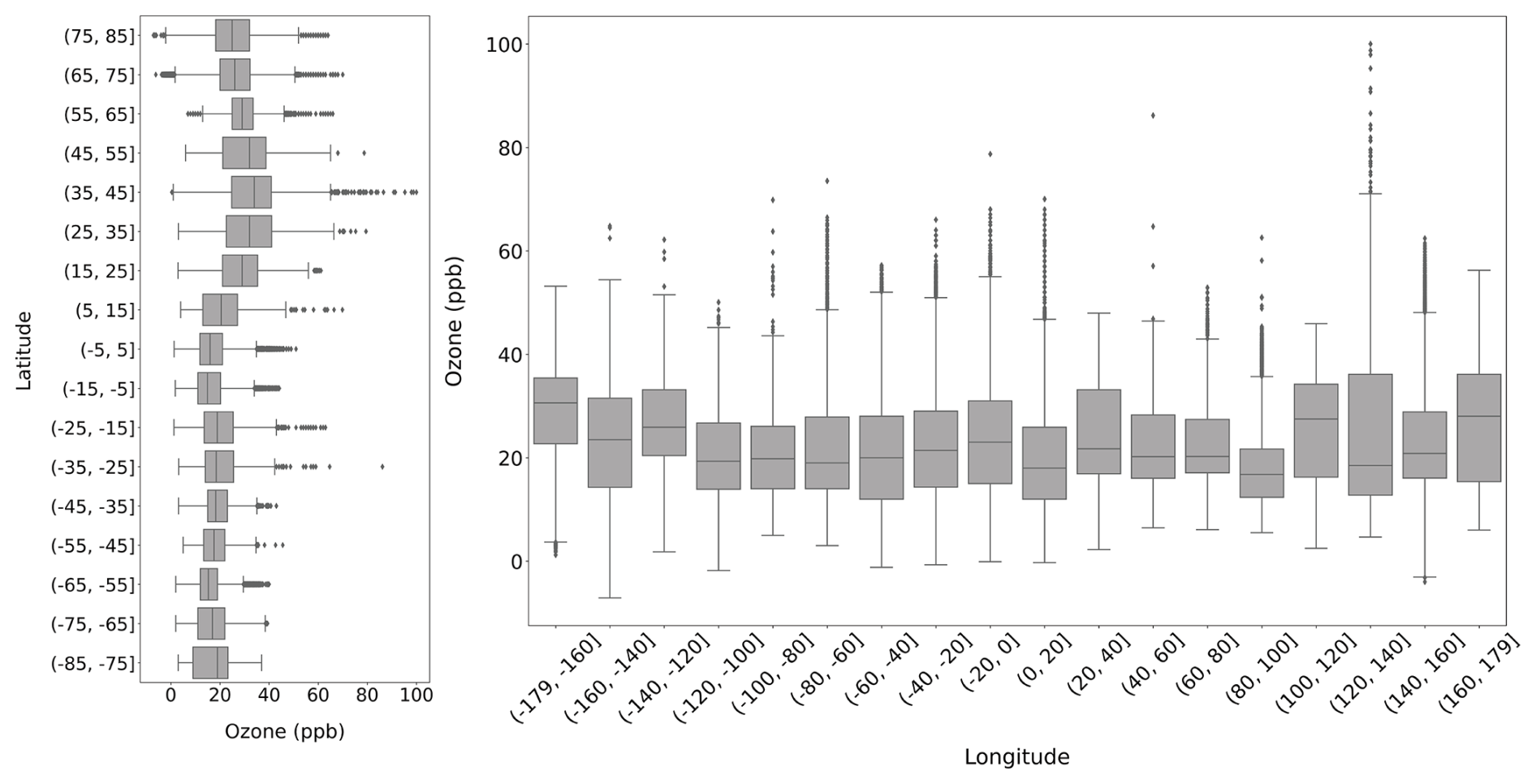
Figure 4 Latitudinal and longitudinal transect of the ship/buoy datasets after filtering for LCL ≥ 72 h.

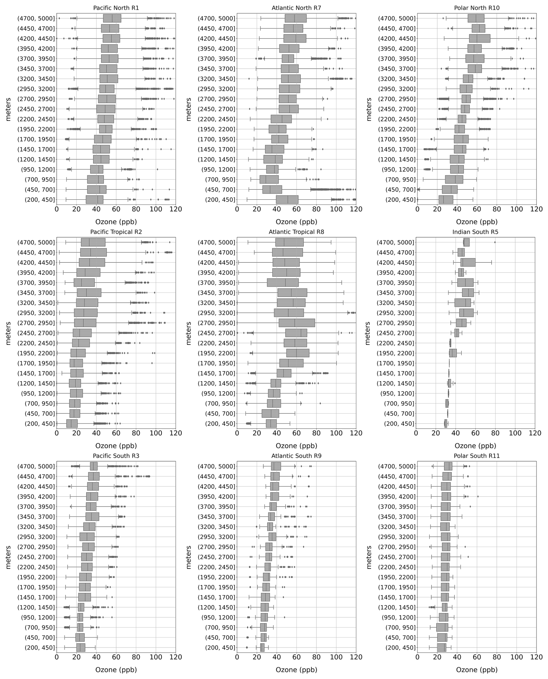
Figure 5 shows the vertical profiles of the combined aircraft and ozonesonde data after application of the LCL72 filter. The data are grouped into 250 m altitude bins. The general tendency is that ozone mixing ratios increase with height, except in R7 (northern Atlantic), where the minimum median values occur in the 700–950 m layer, and in R8 (Tropical Atlantic), where ozone mixing ratios remain nearly constant from 1950 to 5000 m.

Figure 5 Vertical profiles of ozone concentrations by region after filtering for LCL72.

3.2 Seasonal coverage

Table S6 summarizes the number of observation days per region and season. For the ship/buoy dataset, the four seasons were relatively well sampled, but the frequencies were higher for boreal or austral summer than winter for mid- and high-latitude regions (R1, 3, 7, 9, 10, and 11). For the airborne data, coverage was less in summer than in winter over the Pacific, while the opposite was true for the Atlantic. The ozonesonde dataset appeared to have relatively uniform seasonal coverage, except that frequent observations were made during September–October–November over the Antarctic (R11).

3.3 Ship/buoy-based median concentrations and diurnal variation patterns in individual regions (R1–R11)

Table 3 summarizes statistics of hourly data from the ship/buoy dataset (satisfying LCL72) to compare median concentrations across defined regions (R1–R11) and to investigate features of the average diurnal profile (Fig. 6). First, the number of hourly data for individual regions ranged from 3446 (R4) to 61 708 (R10), highlighting the advantage of having this large dataset in one place. For R10 (Arctic), 31 549 and 7732 h of data were from the O-Buoy (autonomous, ice-tethered buoy) and MOSAiC (Multidisciplinary drifting Observatory for the Study of Arctic Climate) missions. The datasets for regions R7–R9 (Atlantic), with contributions from the DWD-MPI cruises, were larger than those for the Pacific (R1–R3). For all regions, the data are almost equally distributed over the time of day. The average diurnal profiles were calculated as follows: local time was derived for each point by adjusting the coordinated universal time (UTC) based on longitude; then, the 25th, 50th, and 75th percentiles were calculated for each hourly bin per region.

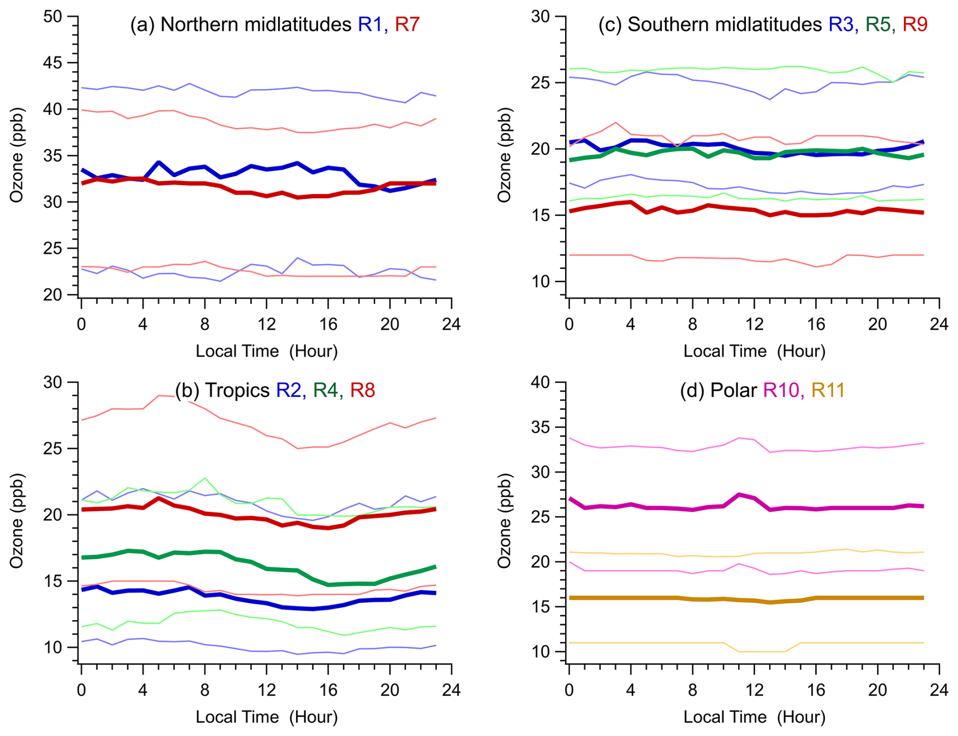
Figure 6 Hourly median (thick lines) and interquartile levels (thin lines) and their diurnal variation by region: (a) R1 and R7 (Pacific and Atlantic northern midlatitudes); (b) R2, R4, and R8 (Pacific, Indian, and Atlantic low latitudes); (c) R3, R5, and R9 (Pacific, Indian, and Atlantic southern midlatitudes); and (d) R10 and R11 (polar, i.e., Arctic and Antarctic regions). The blue, green, and red line colors correspond to the Pacific, Indian, and Atlantic oceans, respectively.

Table 3 Statistics of hourly data from the ship/buoy dataset per defined region (R1–R11).

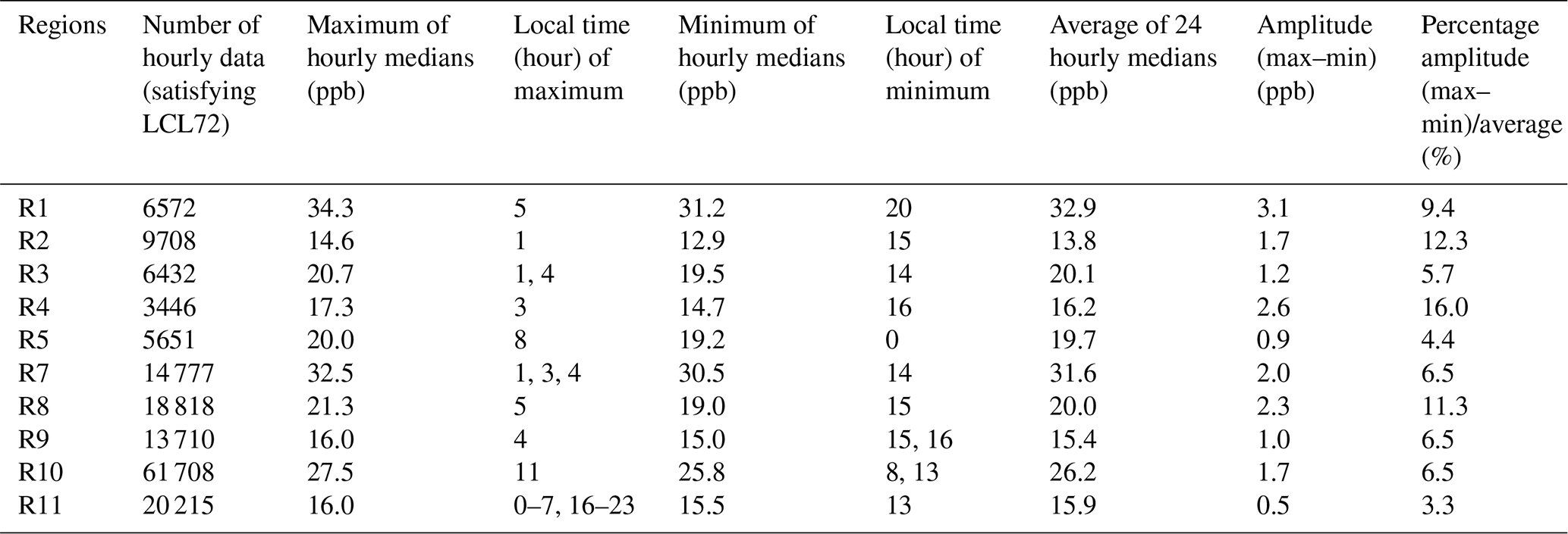
The average of the hourly medians showed variability across regions. For the northern midlatitudes, the Pacific and Atlantic were similar (32.9 and 31.6 ppb for R1 and R7, respectively). For the tropics, the Pacific (13.8 ppb, R2) was lower than the Indian Ocean (16.2 ppb, R4) and the Atlantic (20.0 ppb, R8). For the southern midlatitudes, the values for the Pacific and Indian oceans were similar (20.1 and 19.7 ppb for R3 and R5, respectively), while the Atlantic was the lowest (15.4 ppb for R9). The R9 value is even lower than that of R8 and close to that of R11 (15.9 ppb, Antarctic). R10 (26.2 ppb) was slightly lower than R1 and R7 (northern midlatitudes). While the mixing ratios over the tropics are frequently below 15 ppb (for 30 %, 50 %, and 59 % of the observations over the Atlantic (R8), Indian (R4), and Pacific (R2) oceans, respectively), they are very rarely near zero (<1 % of observations are less than 3 ppb; Fig. 7). This is in marked contrast to the Arctic (R10), where a secondary distribution peak is found at around zero, greater mean and median ozone levels are observed, and only 18 % of mixing ratios are less than 15 ppb. Roughly one-third of these are ozone depletion events (ODEs) and 5.9 % of total observations are below 3 ppb. This indicates that the mechanism(s) of Arctic ODEs is either inoperative or less efficient in the tropics.

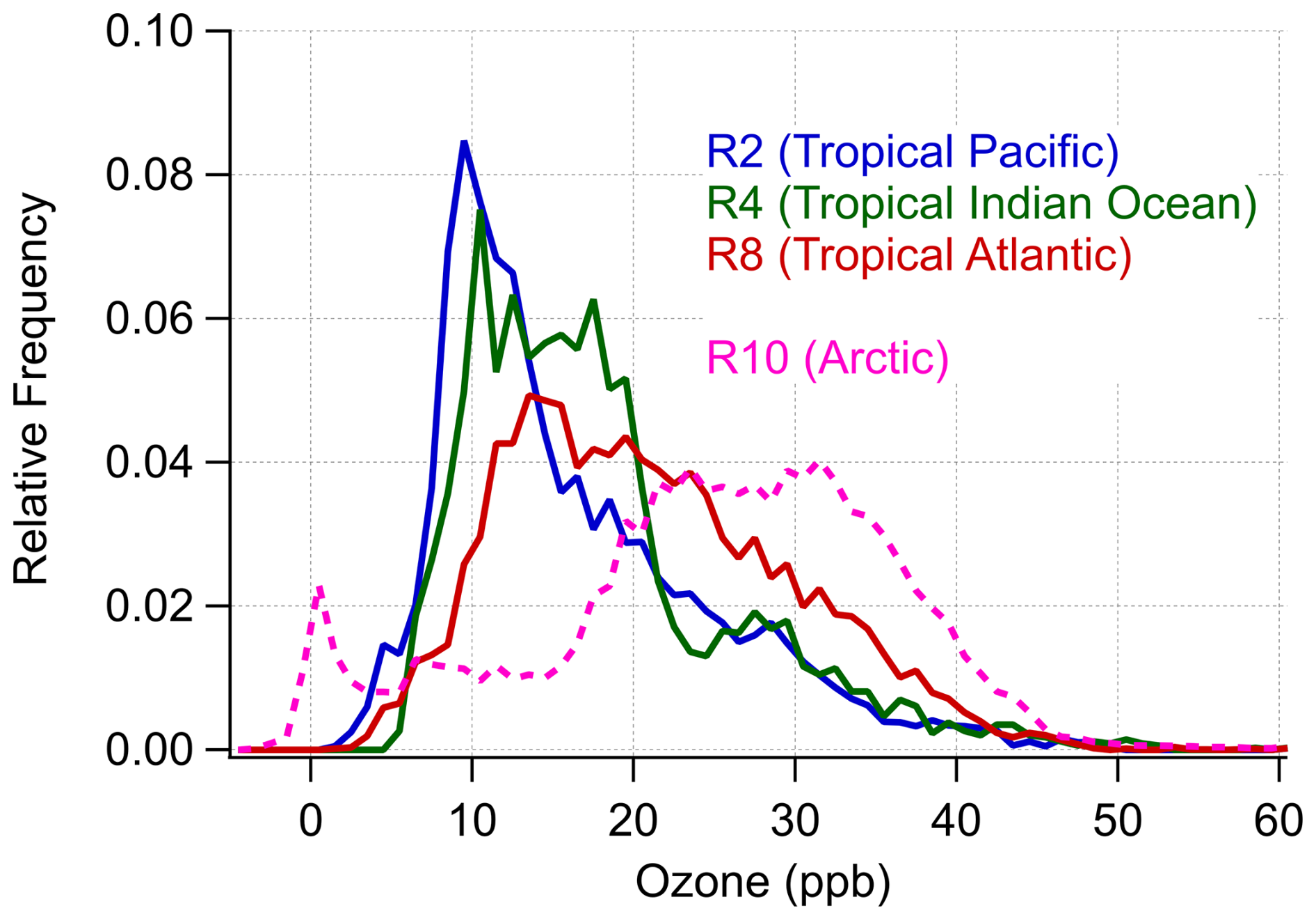
Figure 7 Frequency of observed ozone concentrations in 1 ppb bins computed for ship and buoy observations with LCL ≥ 72 h for tropical regions (Pacific Ocean, R2; Indian Ocean, R4; and Atlantic Ocean, R8) contrasted with the Arctic (R10).

As noted in Sect. 1, a unique feature of ozone in the marine boundary layer over the remote oceans is net photochemical loss. This must result in afternoon decreases in ozone levels. Indeed, flat diurnal patterns or daytime decreases are evident for the ship/buoy data in most regions (Fig. 6, Table 3). The diurnal profiles of the oceanic data suggest that the datasets collected are representative of the marine atmosphere. More specifically, the three tropical regions, R2, R4, and R8, show relatively large daytime decreases. The local time at which the minima were recorded was 15, 16, and 15 h for R2, R4, and R8, respectively (Table 3), while the maxima were recorded at night or in the morning. The different timings must be affected by dynamics and chemistry. The amplitude (maximum minus minimum) of the diurnal variation was 1.7, 2.6, and 2.3 ppb or 12 %, 16 %, and 11 % of the mean concentration for R2, R4, and R8, respectively. Previous studies from ship observations (Johnson et al., 1990; Thompson et al., 1993; Dickerson et al., 1999; Watanabe et al., 2005) and from coastal site observations (Oltmans, 1981; Nagao et al., 1999; Galbally et al., 2000; Read et al., 2008; Hu et al., 2010) have focused on diurnal variation with daytime decreases and reported amplitudes of 1–7.5 ppb (7 %–32 % of average concentration levels). These studies are mainly from single sites/campaigns for short periods of time. Our dataset will be useful to investigate the characteristics of ozone diurnal variations more comprehensively and with statistical robustness. Contributions from various chemical pathways (e.g., HO_x and halogen cycles) will be discussed by comparison with model simulations in the upcoming assessment paper. We also plan an in-depth analysis of our first observational findings, including the substantial reduction in the tropical Indian Ocean (R4), consistent with Dickerson et al. (1999), and the relatively early onset of daytime destruction for R8 and R2.

3.4 Consistency between the ground-based observations and the ozonesonde observations at the same sites

At six stations (Alert, Ny Ålesund, Trinidad Head, American Samoa, Syowa, and South Pole), both ground-based and ozonesonde observations were recorded. The consistency between the two datasets was checked by comparing ozone measurements at ground level and the ozonesonde data at the lowest altitude (typically around 200 m). Figure 8 shows 3-year and 2-year comparisons at Alert and American Samoa, as an example. The agreement was found for cases of episodic ozone decreases in the Arctic and for temporal patterns of variation over days and seasons at both sites, demonstrating the internal consistency of the datasets. Using the ground-based and ozonesonde observations in the Arctic (including Alert) for the year of 2015 as well as ship/buoy/aircraft observations, Gong et al. (2025) discuss the performance of two chemistry transport models. Reasonable agreement was also found with scatterplots for all six sites (Fig. S2), with R² values ranging from 0.64 to 0.95 and slopes of bivariate linear fits ranging from 0.94 to 1.11 when sonde values were plotted against surface observations made within 1 h of each other. This analysis indicated the high quality of the two datasets.

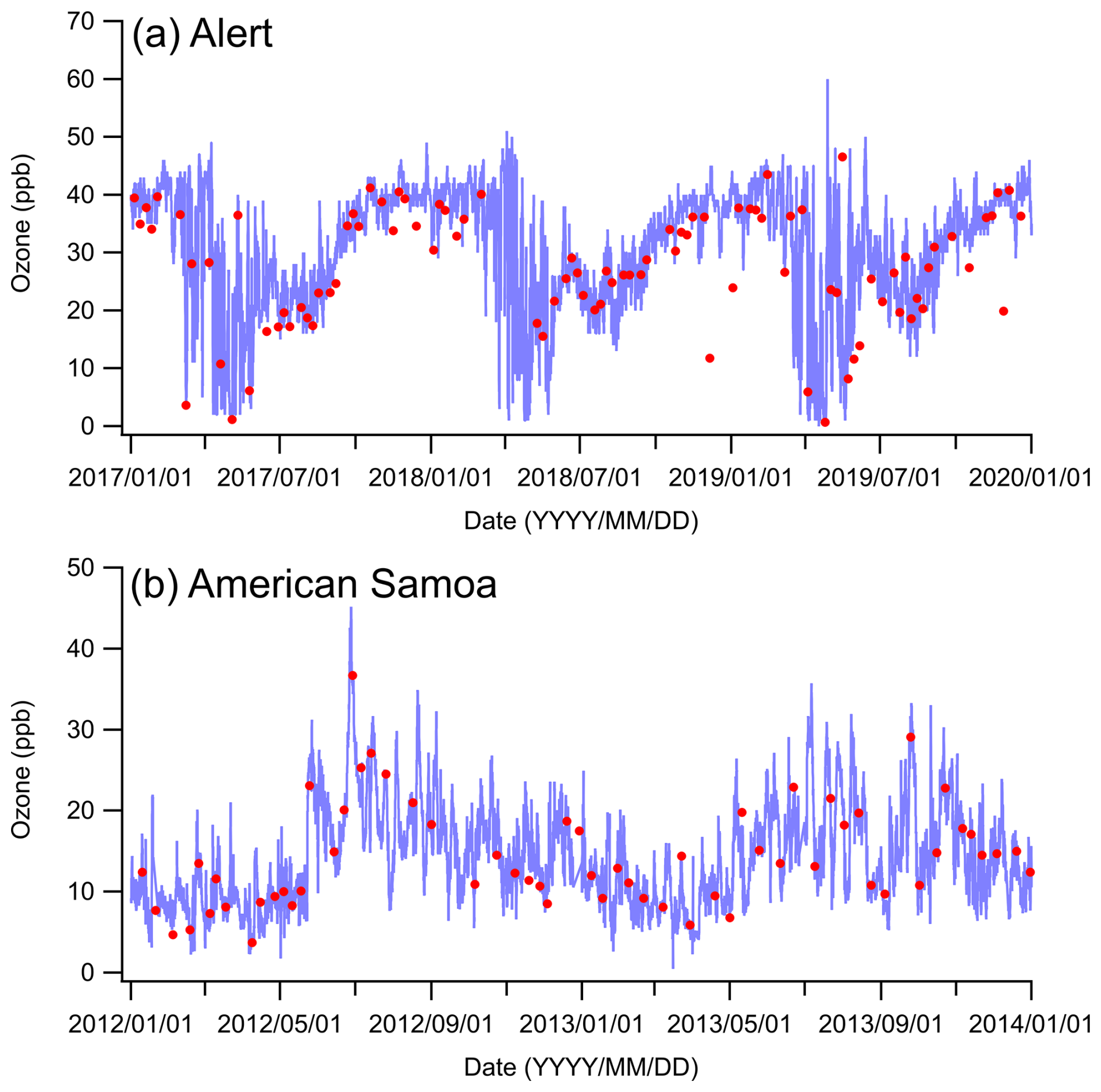
Figure 8 Ozone concentrations from surface observations (blue) and the lowest layer of ozonesonde observations (red, ∼200 m altitude) at (a) Alert and (b) American Samoa.

4 Data availability

The datasets described in this paper are available as five .csv files containing all of the corresponding metadata information. The files are named as follows:

1. toar2_oceans_ship_buoy_data_250203.csv;

2. toar2_oceans_airborne_data_5000m_250203.csv;

3. toar2_oceans_ozonesondedata_250203.csv;

4. toar2_oceans_coastalsites_250203.csv;

5. toar2_oceans_polarsites_250203.csv.

The files contain the key metadata information listed in Tables 1–5 and are available at https://doi.org/10.17596/0004044 (Kanaya et al., 2025).

5 Conclusions and outlook

Under the TOAR-II activity, the Oceans working group has, for the first time, collected and collated observational ozone data over the open oceans and polar regions on a global scale. When available, additional pollution tracers (CO, NO, NO₂, and CN) were also included. All of these datasets are stored in five data files classified by platform type, i.e., ship/buoy, aircraft, ozonesondes, non-polar coastal sites, and polar sites. Here, we describe the datasets and the details of the preprocessing, filtering, and flagging procedures as well as showing basic analyses of the spatiotemporal extent, diurnal variation characteristics, and internal consistency. Our focus was on the ship/buoy and aircraft observations, which contain a total of 208 291 and 424 005 records, respectively. The aircraft and ozonesonde data covered an altitude range from the surface to 5000 m, allowing a complete assessment of ozone over the oceans and polar regions with a focus on the atmospheric boundary layer (<2000 m). All datasets were supplemented with information on the number of hours that each observed air mass was separated from land, derived from backward trajectories. The selected criterion of 72 h or more isolation from land, justified by the coincident radon observations for some selected datasets, allowed the identification of marine air masses. Flat diurnal patterns or diurnal decreases were found after air mass selection, indicating that the collected datasets are representative of the marine atmosphere. Over the tropics, the amplitude of the observed daytime decreases was 11 %–16 %, with the largest decrease observed in the Indian Ocean.

Although the observational data have been collected as widely as possible, they are still not sufficiently dense or homogeneous across the defined regions, particularly for the purpose of small trend detection (Chang et al., 2024). In order to interpret the data, the sampling bias needs to be assessed using atmospheric chemistry transport numerical model simulations (e.g., Sekiya et al., 2020). Despite the inhomogeneity of the observations, point-by-point comparisons with model simulations that match the space and time of the observations are useful for studying key processes and mechanisms. Seasonality and long-term trends in the oceanic and polar ozone observations will be a focus of discussion in the forthcoming assessment (Sommariva et al., 2025).

Appendix A: Acronyms and abbreviations

Table A1 List of acronyms and abbreviations.