Aerial estimates of methane and carbon dioxide emission rates using a mass balance approach in New York State

Accurate greenhouse gas (GHG) emission inventories are vital for climate mitigation as they can identify areas of need and ensure effective policy and regulation in reducing GHG emissions. Several studies have shown that self-reporting GHG inventories are undercounting methane emissions across all anthropogenic sectors, showing an increasing need to validate the inventory with direct measurements. This study carried out aerial observations and emission rates of methane and carbon dioxide across multiple sectors in New York State (NYS). Emission rates were calculated for each of the sources using a mass balance method and were subsequently compared to the 2021 Environmental Protection Agency GHG Reporting Program (EPA GHGRP) Inventory. Landfills were the source of the highest observed methane emission estimates, ranging from 161 to 3440 kg h⁻¹. There was also significant variation in observed emissions within facilities between seasons, indicating a significant influence from meteorology. Variation in estimated measured emissions between different landfills could be due to operational differences. Observed carbon dioxide emission estimates were dominated by combustion facilities, followed by landfills. Comparisons with the inventory show that methane emissions averaged over 10 observed landfills are underestimated by a factor of 2. However, of the 10 landfills, 5 had observed methane emission estimates significantly higher than the inventory value, 4 had an inventory value within the uncertainty range of the observations, and 1 had a landfill-observed emission estimate that was markedly lower than the reported inventory estimate. Seneca Meadows Landfill was the highest emitter from the measurements and was ∼ 4.3× higher than the annual average estimate that was reported to the 2021 EPA GHGRP Inventory. NYS can use this information to inform the NYS GHG Inventory and improve emission estimation methodologies to better depict actual emissions. The two datasets described in this paper are published on PANGAEA. The raw dataset can be found at https://doi.org/10.1594/PANGAEA.979845 (Catena and Smith, 2025a). The emission rate dataset can be found at https://doi.org/10.1594/PANGAEA.979843 (Catena and Smith, 2025b).

1 Introduction

As a leading global greenhouse gas, methane (CH₄) and the reduction thereof have presented themselves as low-hanging fruit in climate change mitigation. This is due to its warming potential of more than 80 times that of carbon dioxide (CO₂) over a 20-year timescale and its relatively short atmospheric lifetime of about a decade as opposed to the longer-lived CO₂, making its mitigation more cost-effective (Shindell et al., 2024; United Nations Environment Programme and Climate and Clean Air Coalition, 2021). There are several natural and anthropogenic sources of methane, with varying contributions to the global methane budget. In New York State (NYS), the largest anthropogenic sources include the fossil fuel, waste, and agricultural sectors, which accounted for 56 %, 29 %, and 15 % of the total state-wide anthropogenic methane emissions, according to the 2021 NYS GHG Inventory (New York State Department of Environmental Conservation, 2023a). It is important to note that the NYS GHG Inventory and recently passed legislation use the 20-year global warming potential (GWP) metric, while most national and international agencies use the 100-year GWP metric. Utilizing the 20-year GWP essentially emphasizes the higher warming impact of methane over 20 years as opposed to over 100 years due to methane's shorter atmospheric lifetime. The 20-year GWP metric yields a much higher relative warming potential, which highlights the urgency in reducing methane over carbon dioxide emissions in the short term.

There are some complexities that arise when trying to accurately assess the contributions from each of the sources of methane; these are primarily due to uncertainties in emission estimations. This uncertainty comes from inadequate measurements and the inconsistent emission estimation results between top-down and bottom-up methods (Saunois et al., 2025). Top-down methods infer emissions through the use of chemical transport modeling and direct, in situ atmospheric measurements over regional or global scales to which they are scaled down to smaller facility- or process-level emissions (National Academies of Sciences, 2018). In contrast, bottom-up approaches are process-based methods, which estimate emissions based on activity data and emission factors (EFs) from individual sources and are extrapolated to regional and national emission totals. These activity data and EFs are a major source of uncertainty in bottom-up GHG inventories because they are not always representative of true emissions, but, given our current understanding, they are considered “best estimates” (Miller and Michalak, 2017; Winiwarter and Rypdal, 2001). Several EFs for various sectors are based on data collected during studies from decades ago, which may not be indicative of current emissions (Lamb et al., 2016; National Academies of Sciences, 2018). In addition to this, since emission inventories are annual averages based on activity data and EFs, they do not account for seasonal or operational changes between facilities, which have been shown to result in significant differences in emissions seasonally and between facilities (Bell et al., 2017; Cusworth et al., 2021, 2024). However, inventories are developed with the information available, and thus a lack of direct measurements of facilities to inform the inventories plays into the highly uncertain emission estimates, which is the case in NYS, where there are few studies of methane observations from major sources of methane.

This high uncertainty in emission inventories has led to a need for verification using top-down direct measurements. Numerous studies have shown that the reporting protocol used to comply with regulations for emission inventories has resulted in undercounting and underreporting of actual emissions across multiple sectors (Bergamaschi et al., 2015; Cusworth et al., 2024; Daniels et al., 2023; Foster et al., 2017; Guha et al., 2020; Lamb et al., 2016; Liu et al., 2023; Moore et al., 2023; Wecht et al., 2014; Yu et al., 2021). Top-down methods can evaluate emission inventories by comparing these inventories with a combination of direct measurements and chemical transport modeling. Top-down constraints afforded by aircraft or satellite observations have been critical in estimating and validating the emission rates of facilities or regions by their ability to sample the whole perimeter of the facility or regional area up to the planetary boundary layer height (Conley et al., 2017; Guha et al., 2020). A mass balance approach of a point source can estimate emissions from aircraft data by applying Gauss's theorem to the reported methane enhancement and observed winds as the aircraft circles in a virtual cylinder around the facility up to the boundary layer height (Conley et al., 2017; Cusworth et al., 2024; Koene et al., 2024). By sampling upwind and downwind of the facility, this allows full characterization of the facility-generated plume (Conley et al., 2017). These top-down estimations may then be compared to the values self-reported to the Environmental Protection Agency (EPA) Greenhouse Gas Reporting Program (GHGRP), which mandates large emitters of GHGs to report their emissions under 40 CFR Part 98 (CFR, 2009). The self-reporting GHGRP is separate from the NYS GHG Inventory in that it provides nation-wide facility-level emission totals, while the NYS GHG Inventory only provides emission source totals across the state (e.g., all landfills or power plants). The NYS GHG Inventory is used for regulatory purposes and allows for tracking and mitigation of state-wide greenhouse gas emissions, while the GHGRP provides facility-specific information and allows for direct comparisons with observations. While it is difficult to make a rigorous comparison between limited observations and the annually averaged inventory, these limited observations help constrain our understanding of emissions from these facilities and highlight any areas in need of further investigation.

In 2019, NYS passed the Climate Leadership and Community Protection Act (CLCPA) that mandates a 40 % reduction in GHG levels by 2030 and an 85 % reduction in GHG levels by 2050 as compared with 1990 levels (New York State Climate Action Council, 2022). In order to achieve these goals, the NYS GHG emission inventory must be accurate since it is the basis for climate policy and regulation. To verify the accuracy of the inventory, aircraft measurements were carried out in NYS at combustion, landfill, wastewater treatment plant (WWTP), and agricultural facilities for comparison with the self-reported GHGRP inventory. This paper reports the observed emission estimation results, which were calculated from a mass balance method using Gauss's theorem across these source sectors. The aircraft emission estimations will be compared with the bottom-up EPA GHGRP Inventory. The results from this paper will help inform the inventory, improve our understanding in estimating accurate emissions, and help NYS meet the goals of the CLCPA.

2 Methods

The aircraft measurements were carried out over two separate field campaigns in June and November/December 2021. With funding from the NYS Energy Research and Development Authority (NYSERDA), the main objective of the study was to determine emission rates from major methane sources in NYS to inform the NYS GHG Inventory. The focus of this study was primarily on methane emissions, but carbon dioxide was also measured as a co-pollutant and is reported in this paper. The aircraft measurements reported in this study were coordinated with a separate study done by Ravikumar et al. (2025), which focused on identifying and estimating methane emissions from natural gas transmission and storage compressor stations in NYS. This study focuses on aircraft sampling over waste incineration, industrial, power plant, waste, and agricultural facilities.

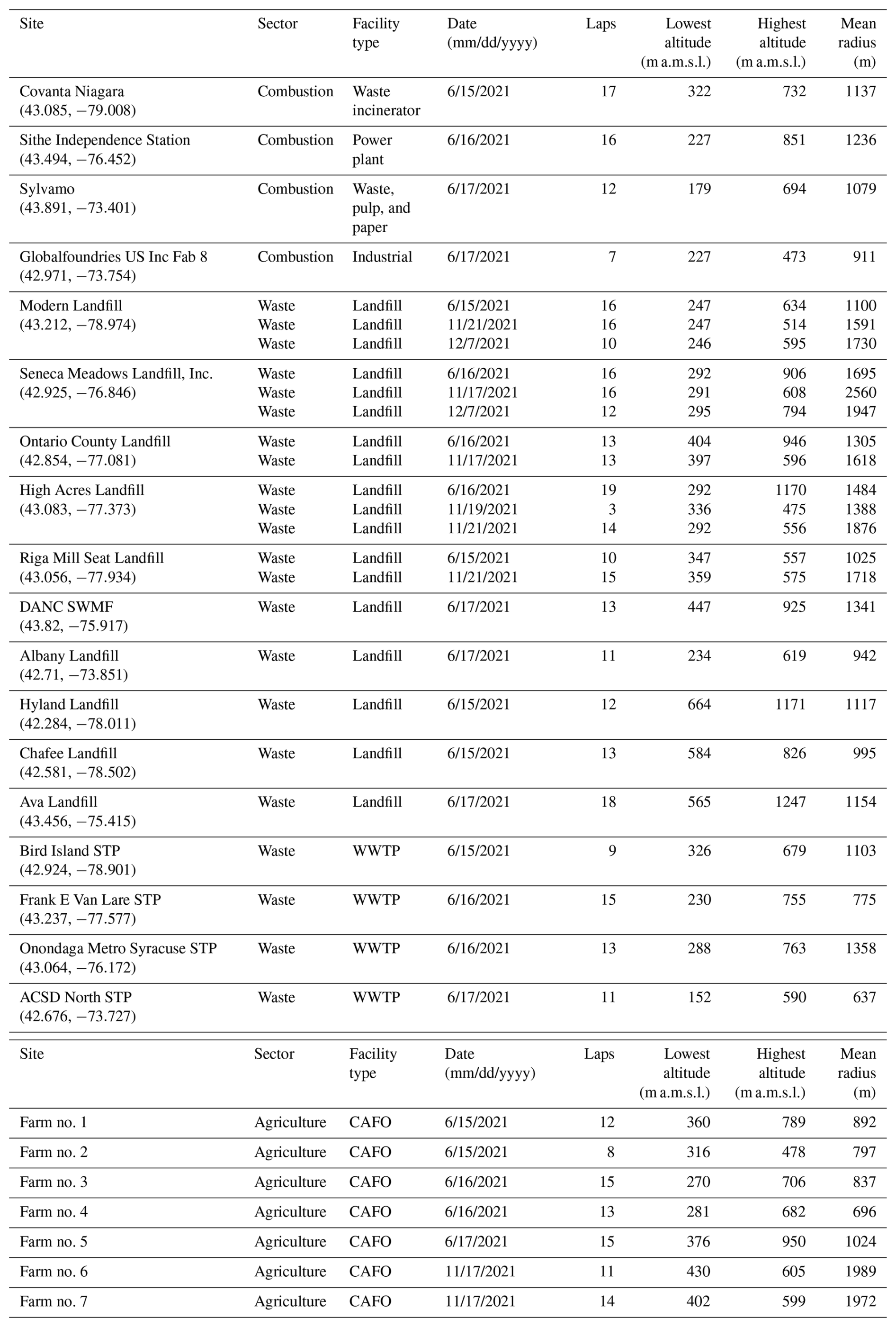
Table 1 lists the facilities sampled along with the facility name, type, date of sampling, number of laps made around each facility, minimum and maximum flight levels, and mean radius of the loops. Figure 1 is a map illustrating all visited facilities for this study. The sites listed in the table were chosen by the project team, which balanced reported and estimated emission rates in the NYS GHG Inventory and their proximity to the airport bases in Rochester and Albany, NY.

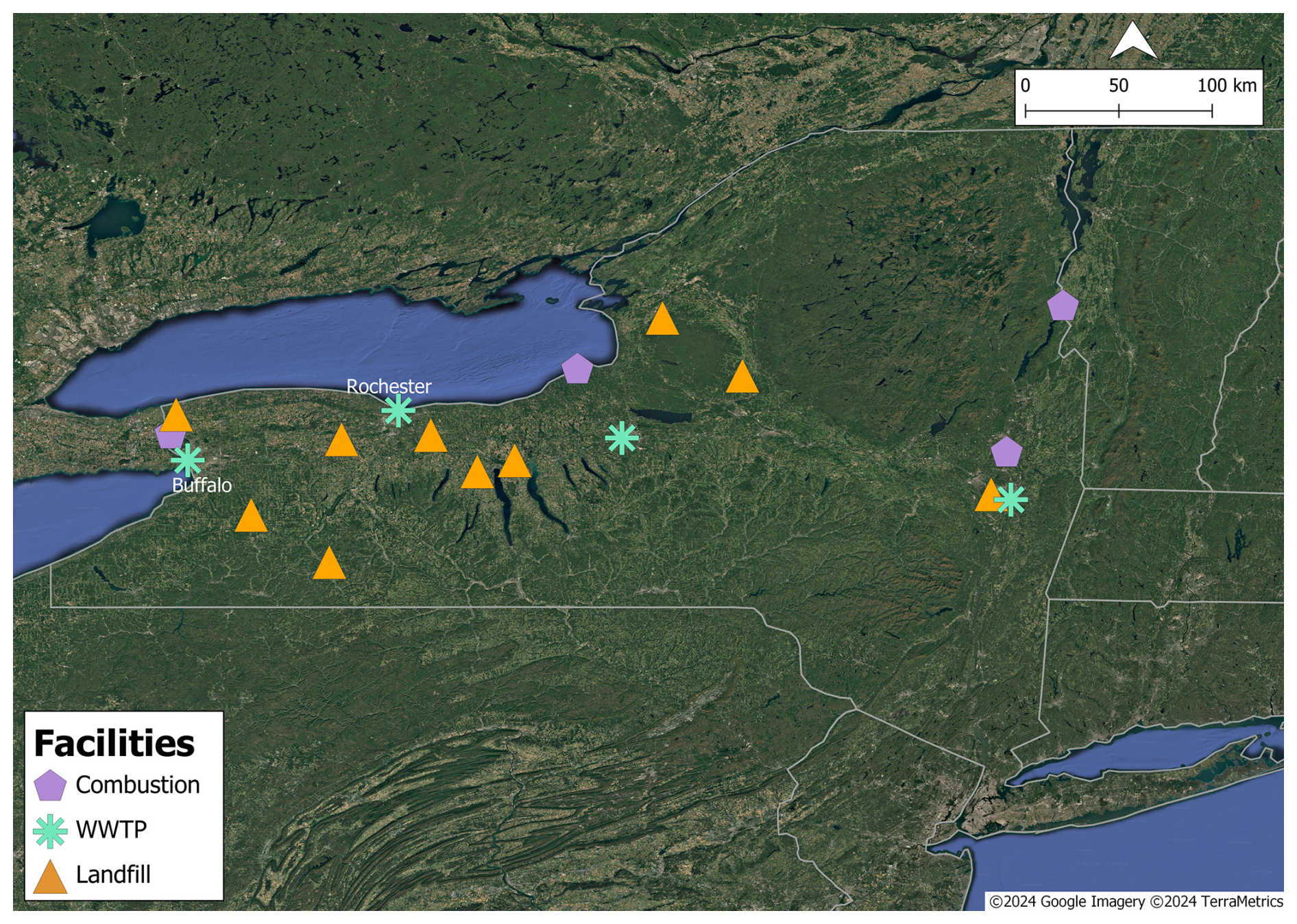
Figure 1 Map of all of the sites sampled in the study, which include combustion facilities, landfills, wastewater treatment plants (WWTPs), and industrial sites. Locations of the concentrated animal feeding operations (CAFOs) sampled are not identified following United States federal privacy laws. The combustion facilities include a waste incinerator plant, a power plant, an industrial facility, and a waste, paper, and pulp facility. This map was created in QGIS (https://qgis.org/, last access: 28 August 2025) using © Google satellite imagery.

Table 1 Information pertaining to all of the sites included in the analysis. The table provides the site name, location, sector, facility type, date of sampling, total number of laps completed around the facility, the lowest and highest altitudes above mean sea level (a.m.s.l.) reached at each facility, and the mean radius of the laps.

The aerial measurements were completed by the Colorado-based scientific research company Scientific Aviation, Inc. (now Champion X), which used a Mooney single-engine-propeller aircraft. There were a total of 25 sites sampled from this study, with 5 sites visited more than once. Additional aircraft missions were flown in the vicinity of New York City, but due to flight restrictions of nearby airports, the aircraft could not sample extensively enough to present reliable fluxes from facilities within the New York City area. Consistent with the Ravikumar et al. (2025) flights, all measurements were taken in the middle of the day from 10:00 to 17:00 local time to ensure that the entirety of the emission plume was captured in a well-mixed and developed boundary layer.

Trace gases were measured by sampling ambient air drawn through rearward-facing inlets mounted on the wing of the aircraft. Observations of CH₄, CO₂, carbon monoxide (CO), and water vapor (H₂O) were recorded using a Picarro G2401 gas analyzer, which is a wavelength-scanned cavity ring-down spectrometer (https://www.picarro.com/environmental/g2401_analyzer_datasheet, last access: 28 August 2025). The analyzer has 1σ precisions of < 1 parts per billion (ppb) of CH₄ and <50 ppb of CO₂ at 5 s. Calibrations were done in flight, along with measurements of temperature and relative humidity by a Vaisala HMP60 probe and GPS coordinates from a Hemisphere high-precision differential GPS. Horizontal wind speed and direction were calculated following the method outlined in Conley et al. (2014). All 1 Hz data were interpolated. Further descriptions and discussion of the Scientific Aviation aircraft, analyzer precision and accuracy, and data met can be found elsewhere (Conley et al., 2017; Karion et al., 2015; Peischl et al., 2016; Ravikumar et al., 2025; Smith et al., 2015).

2.1 Mass balance emission estimation

Emission estimates for each sampled facility were calculated from a mass balance method using Gauss's theorem (Conley et al., 2017; Ravikumar et al., 2025). As the aircraft flies in a spiral pattern defining a virtual cylinder above the facility, the total flux contribution from the facility is estimated from the product of the methane observations and the horizontal wind flow and is summed over each height level. The total contribution from the facility is estimated by integrating the outward horizontal flux at each point along the flight path. This is done by following the mass balance equation below (Conley et al., 2017):

$$\begin{array}{}\text{(1)}& Q_c=〈{\displaystyle \frac{\partial m}{\partial t}}〉+\underset{\mathrm{0}}{\overset{z_{max}}{\int }}\oint c^{\prime }{\mathit{u}}_{\mathrm{h}}\cdot \widehat{\mathit{n}}\mathrm{d}l\mathrm{d}z,\end{array}$$

where Q_c is the emission rate, z_max is the top of the sampling height, and c^′ is the deviation from the mean concentration for each loop such that $C=\stackrel{\mathrm{‾}}{c}+c^{\prime }$, where C is the measured concentration and $\stackrel{\mathrm{‾}}{c}$ is the mean concentration per loop, u_h is the horizontal wind vector, $\widehat{\mathit{n}}$ is the outward-pointing unit vector, dl is the change in length per sample, and dz is the change in height between each loop around the facility. The volume mixing ratio is converted into a mass mixing ratio using the ideal gas law and is then multiplied by the altitude-dependent density to obtain the mass concentration. The storage term, $〈\frac{\partial m}{\partial t}〉$, is calculated as the time rate of change in the average mass concentration within the sampled volume throughout the entire period of measurement. Numerically integrating Eq. (1) yields Eq. (2) (Conley et al., 2017):

$$\begin{array}{}\text{(2)}& Q_c={\displaystyle \frac{\mathrm{\Delta }m}{\mathrm{\Delta }t}}+\sum _{z=\mathrm{0}}^{z=Z_{max}}\left(\sum _{\mathrm{0}}^L(\mathit{\rho }\cdot c^{\prime }\cdot {\displaystyle \frac{{\mathrm{MW}}_{{\mathrm{CH}}_{\mathrm{4}}}}{{\mathrm{MW}}_{\mathrm{AIR}}}}\cdot u_{\mathrm{n}})\cdot \mathrm{\Delta }s\right)\cdot \mathrm{\Delta }z.\end{array}$$

The second term in Eq. (2), the net outflow term, estimates the contribution from the facility by summing the product of the scalar air density (ρ) as a function of height, the wind speed normal to the flight path (u_n), the fraction of the molecular weight of methane to air $\left(\frac{{\mathrm{MW}}_{{\mathrm{CH}}_{\mathrm{4}}}}{{\mathrm{MW}}_{\mathrm{AIR}}}\right)$, and the change in distance between each time step over the distance of one entire loop (L). This calculates a total product sum for each loop. The loops are then aggregated into six equal-height bins from the lowest (z=0) to highest flight levels ($z=Z_{max}$). The lowest layer extended from the lowest measured flight altitude to the surface, which varied from site to site. For loops within the same height bin, the total product sum from those loops was averaged. The total product sum was then multiplied by the height bin width (Δz) and summed over each height bin.

The remaining term in Eq. (2) is the storage term, which is estimated using the time rate of change of the average mass concentration from loop to loop over the full flight. The area is determined by applying the Convex Hull function in Python to the measured x and y coordinates, which are then multiplied by the maximum measured altitude above ground level to estimate the total volume. The rate of change, or slope, is determined from the average mass concentration from each loop with time (kg m⁻³ s⁻¹) and is then multiplied by the volume of the sampled area to get the rate of change of the mass concentration over the entire period of measurements at the given facility. This total rate of change or storage term is then added to the net outflow term from Eq. (2) to get the net total emission rate (Q_c) of the facility. Typical average values of the dl and dz terms are ∼ 70 and ∼ 72 m, respectively. The spiral pattern of the aircraft led to an average variation of ±17 m in height within each loop.

The Conley et al. (2017) study assumed near-zero vertical mixing at the top of the plume, which was proven to be an accurate assumption, as shown in the first figure of their paper. Figure 2 below depicts a typical flight pattern from this study and the measured methane mixing ratio profile at Seneca Meadows Landfill on 16 June 2021. Since the methane mixing ratio decreased to background levels at the highest flight level above the plume, the assumption of Conley et al. (2017) held true for this study as well.

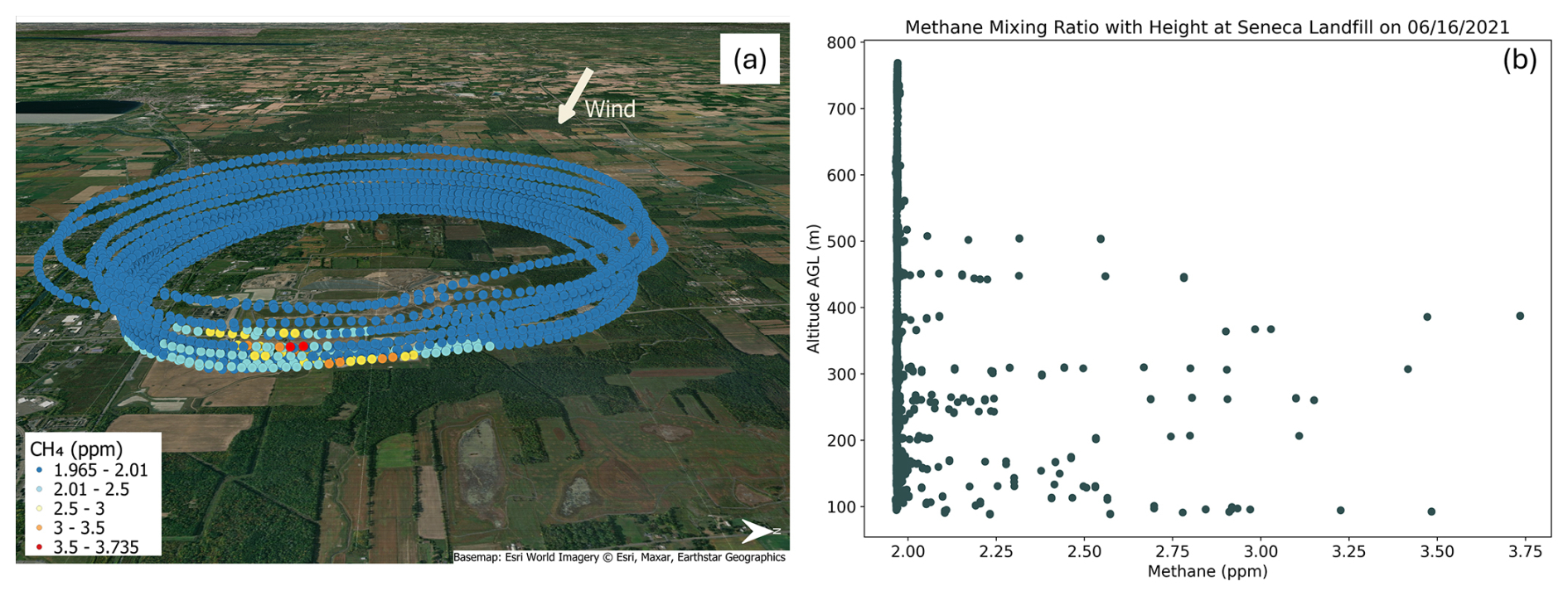
Figure 2 Panel (a) on the left depicts the flight path around Seneca Meadows Landfill on 16 June 2021. Methane mixing ratios in parts per million (ppm) were measured at multiple altitudes with varying concentrations. Panel (b) on the right is a profile of the observed methane plume.

2.2 Sources of uncertainty

There are several sources of uncertainty with the mass balance approach using Gauss's theorem, including measurement error, wind parameterization from a moving aircraft, convective boundary layer height determination, interpolation of data, and pinpointing of exact sources of interest without the interference of additional sources nearby (Cambaliza et al., 2014). Another major source of uncertainty in this method is the section of the plume that is not accounted for from the ground level up to the lowest flight level (Cambaliza et al., 2014; Gordon et al., 2015). Assuming a well-mixed boundary layer, the methane mixing ratio is assumed to be constant from the surface up to the lowest flight level. Conley et al. (2017) analyzed several distances to the point source to determine the most ideal sampling distance. This consisted of determining a balance between being far enough from the source to ensure that the near-surface plume mixed well enough into the boundary layer with limited variability and close enough where there was a discernable difference between the plume and background. This sampling distance method was used for this study with a combination of the convective boundary layer height, standard deviation of the wind speed, and parameterization for the convective velocity scale, as done in Conley et al. (2017). There is also the issue of additional unintended sources included in the analysis in urban areas due to a higher number of adjacent sources, making it difficult to focus on one specific facility. Error could arise from either an additional source nearby or the inability to sample the complete background concentration upwind. Another challenge with these direct measurements is the lack thereof. These observations were only made on a few days of the year, which can lead to bias as they do not account for seasonal or operational changes and may not be representative of an annual emission rate. At the same time, these are the only observations available for these facilities, and they help bridge the data gaps of more reliable observations. These measurements were also performed during the daytime, which precludes consideration of any diurnal variation. This can also lead to error as previous studies have shown measurable diurnal variation in concentrations due to pressure changes, temperature, wind shear, and varying convective layer heights, especially from landfills (Delkash et al., 2022; Xu et al., 2014). However, the intensity of diurnal variation influences is mostly dependent on landfill management, such as methane generation rate, cover types of landfills, gas collection, and climate (Delkash et al., 2022).

Uncertainties are estimated following the method outlined in Erland et al. (2022), which accounts for measurement error, the variability in the flux between height levels, and how stationary the plume is (Conley et al., 2017; Erland et al., 2022). The standard deviations between the heights are summed in quadrature to get the total uncertainty. The error in extrapolating to the surface is accounted for when estimating error from flux variation and is estimated as twice that of the error estimated for the lowest height bin (Erland et al., 2022). Referring to Tables 2, 3, and 4, which list the observed emission rates and their uncertainties for all of the sectors, the combustion facilities had a methane emission uncertainty average of about 48 %, ranging from 18 % to 82 %. Landfills had ∼ 30 %, ranging from 10 % to 80 %. WWTPs showed much higher variation in uncertainty, ranging from 34 % to 1330 %. Uncertainty for concentrated animal feeding operations (CAFOs) averaged about 60 %, ranging from 32 % to 111 %, not including one farm which had an uncertainty of ∼ 300 %. These uncertainties are an estimate of the variation of the flux between each of the loops around a particular site only, which mostly takes into account the turbulent effects on the plume. They do not include any other potential source of uncertainty, including day-to-day or seasonal differences.

3 Results

3.1 Emission rate comparisons

The calculated emission rates from the aircraft observations and Eqs. (1) and (2) for the combustion, landfill, WWTP, and agricultural sources can be seen in Tables 2, 3, and 4, respectively. Observed emission rates were calculated for CH₄ and CO₂ for each of the facilities. Tables 2 and 3 also list the available self-reported 2021 EPA GHGRP Inventory CH₄ and CO₂ estimates. The EPA GHGRP Inventory methane estimates are converted from the carbon dioxide equivalent using the 100-year GWP values from the Intergovernmental Panel on Climate Change (IPCC) Fourth Assessment Report (IPCC, 2007; US EPA, 2022). The only facilities as part of this study required to report methane emissions to the EPA GHGRP Inventory are the landfill and combustion facilities. Hence, there are no available comparisons between the observations and self-reported inventory values for the WWTP and CAFO facilities. Comparisons with the EPA GHGRP Inventory are discussed in Sect. 3.2.

Observed methane emission rates varied widely both between and within the combustion, landfill, WWTP, and agricultural sectors. As seen in the comparison plots in Fig. 3, landfills were responsible for the highest observed methane emission rates ranging from 161 to 3440 kg h⁻¹, with an average of 1240 kg h⁻¹. The large range in values between the facilities can be due to several factors, including operational differences, sizes of landfills, or waste quantity. Seneca Meadows Landfill accounted for the largest observed methane emission estimate, which is consistent with its status as the largest landfill in New York State in terms of both current size and annual permits (New York State Department of Environmental Conservation, 2020).

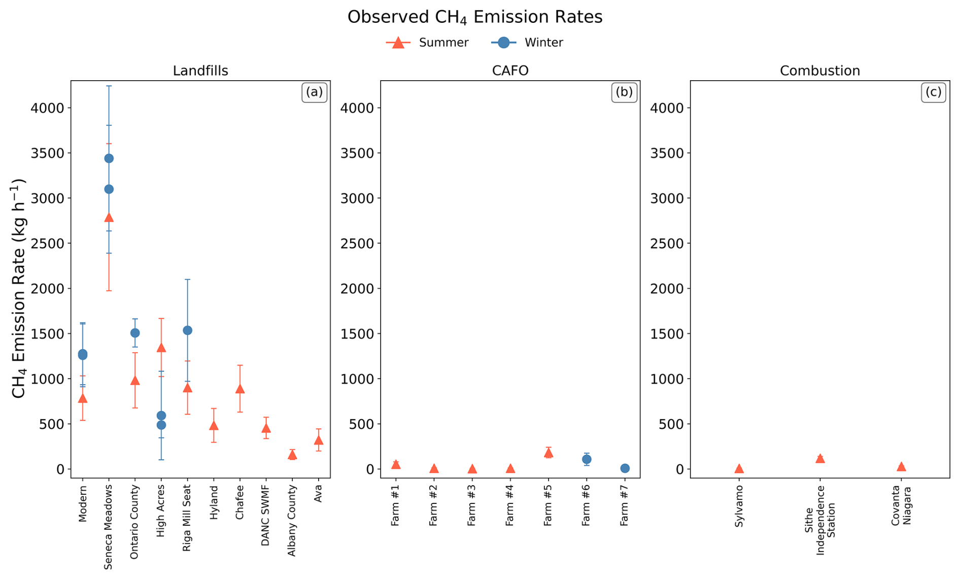
Figure 3 Observed methane (CH₄) emission rate comparisons between each of the sectors for (a) landfills, (b) CAFOs, and (c) combustion facilities. The wastewater treatment plants' observed emission rates were not included due to unreliable and low emissions.

There was also a large range of values within the facilities that were sampled more than once, and every one of the facilities exhibited higher emission estimates in the winter months compared to the summer months, except for High Acres Landfill, which showed the opposite. Between the summer and winter months, there were differences in the methane emission estimates of approximately 45 % at Modern, 42 % at Ontario County, 85 % at High Acres, and 52 % at Riga Mill Seat Landfill. Seneca Meadows Landfill was the only facility with relatively consistent emission rates, showing a ∼ 15 % difference between the summer and winter months. Variation in meteorological and environmental conditions, such as the ambient pressure and temperature, wind, and soil moisture and temperature of the landfill, has been shown to impact methane emissions from landfills, which can explain the seasonal differences in observed emission rates at these landfill facilities (Delkash et al., 2016, 2022; Poulsen et al., 2003; Rachor et al., 2013; Xu et al., 2014; Zhang et al., 2013). While these studies have shown seasonal influences on methane emissions, the results here only provide 1 d each from each season, which may leave out other possible influences like synoptic-scale disturbances or operational differences.

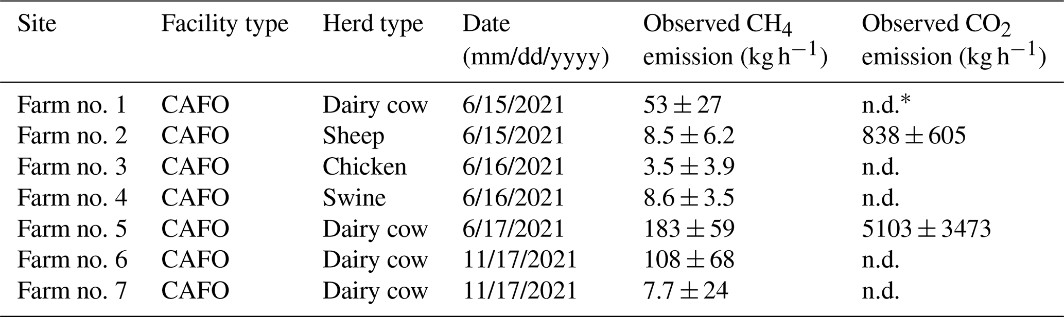
There were several facilities that exhibited non-detectable or non-quantifiable observed emission rates, which can be for several reasons, including the inability to detect an upwind background and downwind enhancement, quantify a plume within variable winds, or detect the facility location within an urban area with adjacent sources nearby. WWTPs showed mostly lower emission rates than landfills, ranging from 12.8 to 21.6 kg h⁻¹. Of the 5 WWTP sampling days, three samples had non-detectable fluxes, likely due to the fact that they were located in urban areas and the aircraft was unable to get close enough to the ground to sample the plume from the urban background. CAFOs and the combustion facilities exhibited comparable ranges of methane estimates between each other of 3.5–182.8 and 6.7–118 kg h⁻¹, respectively. The large variation in the CAFOs could be for a number of reasons. The CAFOs had different types of herds (i.e., dairy cows, swine, sheep, and chickens), which would result in varying emissions (EPA, 2024). Although the largest farms were sampled, the exact herd size enclosed within the flight loops during sampling was not known since a particular farm could have several locations and the central operating location given in the database does not always mean that the herd is at that location. Lastly, manure management is a large source of methane within the livestock sector and is usually stored in lagoons away from barns or central operating locations, which could potentially leave it out of the area sampled by the aircraft and ultimately exclude it from the emission rate estimate.

As expected, the Sithe Independence Station natural gas power plant and Covanta Niagara waste incineration facility had by far the largest observed CO₂ emissions with maximum emission rates of 300 000 and 129 783 kg h⁻¹, respectively, but emissions from landfills were still quite substantial and larger than the remaining sources with a maximum emission rate of 58 941 kg h⁻¹, which can be seen in Fig. 4.

Figure 4 Observed carbon dioxide (CO₂) emission rate comparisons between each of the sectors for (a) landfills, (b) WWTPs, (c) CAFOs, and (d) combustion sources. The power plant and waste incinerator facilities were not included in this plot due to the significantly higher emission estimates.

Table 2 Observed methane (CH₄) and carbon dioxide (CO₂) emission rates and their uncertainties from the waste incineration, power plant, industrial, and waste, paper, and pulp sector facilities in comparison to the available 2021 Environmental Protection Agency GHG Reporting Program (EPA GHGRP) Inventory value.

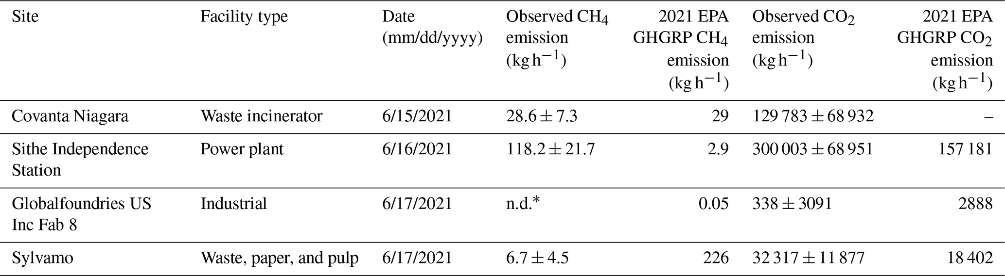
^* n.d. – not detected.

Table 3 Observed CH₄ and CO₂ emission rates and their uncertainties from the landfill and wastewater treatment plant sector facilities in comparison to the available 2021 EPA GHGRP Inventory values.

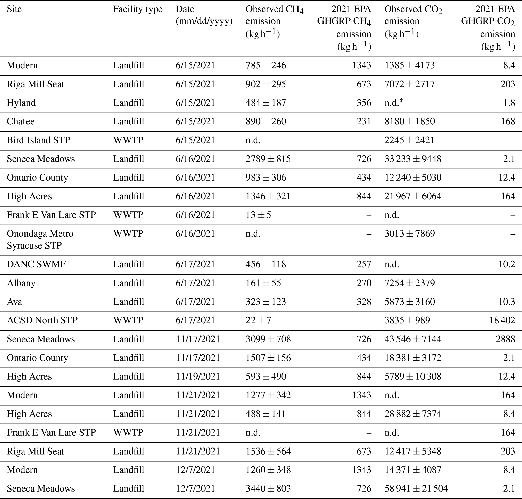
^* n.d. – not detected.

Table 4 Estimated emission rates from the agricultural sector facilities for CH₄ and CO₂, together with their uncertainties. The EPA GHGRP Inventory is not available for CAFOs.

^* n.d. – not detected.

3.2 2021 EPA GHGRP CH₄ emission inventory comparisons

The methane emission estimates from this study have been compared to available methane emission rates self-reported to the EPA GHGRP (US EPA, 2022). As mentioned previously, facility-level methane emission rates are not available in the 2021 NYS GHG Inventory (New York State Department of Environmental Conservation, 2023b). The comparisons between the methane observations from this study and the self-reported EPA GHGRP Inventory can be seen in Tables 2 and 3 and Fig. 5. As seen in Table 3, the observed landfill emission estimates were, on average, 2 times greater than what was reported in the inventory. The highest observed emission rates were estimated from Seneca Meadows Landfill to range from 2789 to 3440 kg h⁻¹ and were ∼ 4.3 times greater than the GHGRP self-reported value of 726 kg h⁻¹. Modern Landfill self-reported as the highest in-state point source emitter of methane at 1343 kg h⁻¹, yet the average observed estimate from the facility (∼ 1107 kg h⁻¹) was lower than the inventory estimate. Nonetheless, the inventory estimate is still within the uncertainty range of the observed estimate rate at Modern Landfill, which is the case for other three landfills as well, i.e., High Acres, Hyland, and Ava. Albany Landfill was the only one where the observed CH₄ emission rate was relatively lower than the self-reported inventory value, i.e., about 60 % of the self-reported value. The five remaining landfills, i.e., Seneca Meadows Landfill, Ontario County Landfill, Riga Mill Seat Landfill, Chafee Landfill, and Development Authority of the North Country (DANC) Solid Waste Management Facility, all exhibited higher observed CH₄ emission estimates than what was reported in the inventory, averaging ∼ 3.1 times greater. As seen in Fig. 5b, the methane emission rates varied widely between the combustion facilities for both the observed and inventory estimates. The differences were also inconsistent – the Sylvamo Paper Mill mass balance estimate was ∼ 34 times lower than the inventory's, while the Sithe Independence Station mass balance estimate was ∼ 41 times greater than the inventory's. Figure 5 also shows the significantly higher methane emission rates from landfills over the combustion facilities. As seen in Table 3, the CO₂ emission rate comparisons between the observed and self-reported GHGRP values are significantly different at the landfill facilities due to the EPA not accounting for biogenic CO₂ emissions. The inventory only accounts for combustion-related emissions of CO₂.

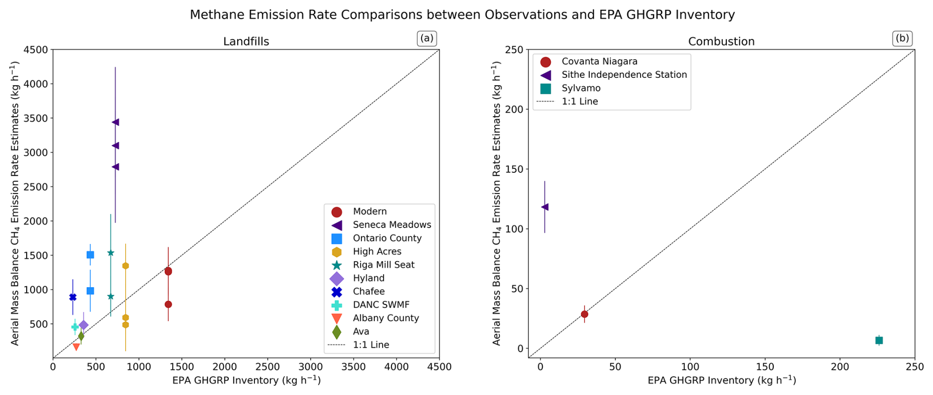
Figure 5 Comparisons between the methane emission rates estimated from this study and the 2021 EPA GHGRP Inventory at each of the landfills (a) and combustion facilities (b) visited during the study.

These results suggest that the self-reporting of methane emissions from landfills in NYS may be underestimated. However, there are a few cases where the GHGRP values are higher than the observations suggest. This inconsistent comparison with the inventory likely results from the assumptions by each landfill operator about the methane captured (all the landfills sampled employ methane capture technologies). Additionally, the discrepancies between the observed and reported values seen here echo what has been reported from previous studies, which is mostly due to differences in estimating the emission rate between top-down and bottom-up approaches (Saunois et al., 2025). While this could explain the disagreement seen here between the observations and the reported values, the mostly higher observations from this study follow a similar trend seen in other recent studies, which suggest that the methods followed in the inventory may not be accounting for all emissions (Bergamaschi et al., 2015; Cusworth et al., 2024; Daniels et al., 2023; Foster et al., 2017; Guha et al., 2020; Lamb et al., 2016; Liu et al., 2023; Moore et al., 2023; Wecht et al., 2014; Yu et al., 2021). However, there is some issue with trying to compare the two when they may not be direct comparisons. The self-reported values are based on annual numbers, which can lead to uncertainties and inaccuracies in emission inventories due to the effort in trying to consolidate the emission estimate into a single annual average rate and thus not accounting for seasonal and operational differences. By contrast, individual observed emission rates may not be a direct comparison with the inventory estimates, since they are a snapshot from a few days of the year as compared with the annual average from the inventory and may not be representative of typical emissions. At the same time, these limited observations provide valuable constraints and data informing our understanding of methane emissions. A more equivalent comparison can be made through long-term measurements of methane emission rates from satellite observations or possibly from continuous facility-specific ground-based measurements, and we recommend that such future studies be performed.

4 Data availability

All data described in this paper can be accessed from PANGAEA at the following two DOIs for the raw data (https://doi.org/10.1594/PANGAEA.979845, Catena and Smith, 2025a) and the emission rates (https://doi.org/10.1594/PANGAEA.979843) (Catena and Smith, 2025b).

5 Conclusion

Aircraft observations were carried out for this study to estimate methane and carbon dioxide emission rates from facilities across the combustion, landfill, WWTP, and agricultural sectors. A total of 25 sites were sampled, with measurements made in June and November/December 2021. Emission rates were calculated using a mass balance method by applying Gauss's theorem to the observed mixing ratios and horizontal wind. Landfills were responsible for the highest estimated methane emission rates ranging from 161 kg h⁻¹ at Albany County Landfill to 3440 kg h⁻¹ at Seneca Meadows Landfill. There were large variations in methane emission estimates both among and within the facilities between seasons. The combustion and landfill facilities had the highest CO₂ emission rates, with the Sithe Independence Station natural gas power plant significantly having the highest one at 300 000 kg h⁻¹. The self-reporting EPA GHGRP Inventory, on average, generally undercounts methane emissions from landfills by a factor of 2. However, there are a few facilities where the inventory overestimates this. From the 10 landfills sampled, five observed methane emission rates were higher than those of the inventory, four were within the uncertainty range, and the remaining landfill observed a lower emission rate than the inventory. These differences can be attributed to a number of factors, including operational differences or seasonal influences. However, this study does not provide sufficient data and information to determine both the reason for the differences and the true emission rate. Long-term continuous monitoring is crucial for establishing accurate and reliable emission estimates to better inform the NYS GHG Inventory and policy aimed at climate mitigation. However, the results from this study provide valuable and very much needed information on methane sources and their emissions in NYS.