A global classification dataset of daytime and nighttime marine low-cloud mesoscale morphology based on deep-learning methods

Marine low clouds tend to organize into larger mesoscale patterns with distinct morphological appearances over the ocean, referred to as mesoscale morphology. While previous studies have mainly examined the fundamental characteristics and shortwave radiative effects of these mesoscale morphologies, their behaviour in the nighttime marine boundary layer (MBL) remains underexplored due to limited observations. To address this, we established a global classification dataset of daytime and nighttime marine low-cloud morphology using a deep residual network model and infrared radiance data of 1° × 1° resolution from the Moderate Resolution Imaging Spectroradiometer (MODIS), with machine-learning-retrieved all-day cloud optical thickness aiding in model training. We analysed day–night contrasts in climatology, seasonal cycles, and cloud properties of different cloud morphology types in this study. Results show that the relative frequency of occurrence of closed mesoscale cellular convection (MCC) increases significantly at night, while that of suppressed cumulus (Cu) shows a remarkable decrease. Disorganized MCC and clustered Cu display a slight frequency increase at night. In addition, solid stratus and three MCC types exhibit distinct seasonal variations, whereas two cumuliform types show no clear seasonal cycle. Our dataset extends the study of mesoscale cloud morphologies from daytime to nighttime, and the 1° × 1° resolution makes it a better match with other climate datasets. It will provide an important foundation for further research on the interactions between cloud morphology and climate processes. The final cloud classification dataset and the model development datasets are open-access and available at https://doi.org/10.5281/zenodo.13801408 (Wu et al., 2024).

1 Introduction

Marine low clouds cover the vast area of the oceans and have a pronounced impact on Earth's radiation budget. They exert strong radiative cooling on the planet as the residual of a larger cooling effect and a positive warming effect (Klein and Hartmann, 1993; Eytan et al., 2020). These radiative effects are known to be sensitive to cloud types due to their different cloud properties, such as cloud fraction and albedo. Traditional ground-based observations have classified individual marine low clouds using the cloud types defined by the World Meteorological Organization (WMO), such as cumulus (Cu), stratocumulus (Sc), and stratus (St) (Zhang et al., 2018; Li et al., 2022; Guzel et al., 2024). However, satellite imagery shows that these individual clouds tend to organize into larger mesoscale patterns with distinct morphological features that are not easily discernible from the limited perspective of ground observation instruments. These mesoscale cloud patterns, referred to as cloud mesoscale morphologies, have been shown to exert different radiative effects on the climate (McCoy et al., 2017, 2023; Mohrmann et al., 2021) and also to reflect the intricate physical processes of the underlying marine boundary layer (MBL) (Wood, 2012; Bony et al., 2020; Eastman et al., 2022; Zhu et al., 2024; Mohrmann et al., 2021).

Previous studies have identified several critical environmental factors that influence the evolution of marine low-cloud morphologies. Open and closed mesoscale cellular convection (MCC) clouds are both affected by cloud-top longwave radiation cooling (Wood, 2012), but the surface fluxes dominate the open MCC when there is a strong cold advection such as a polar outbreak. As a result, the passages of mid-latitude cold-air outbreaks serve as key triggers for the transition from closed to open MCCs (McCoy et al., 2017; Tornow et al., 2021). In the subtropics, precipitation promotes the organization and sustainment of open cell structures and dominates the transformation from closed to open MCC clouds (Savic-Jovcic and Stevens, 2008; Feingold et al., 2010; Yamaguchi and Feingold, 2015; Eastman et al., 2022). In contrast, closed MCC tends to evolve into more disorganized cumulus under conditions of warmer sea surface temperatures and increased entrainment of dry air at the cloud top (Eastman et al., 2022; McCoy et al., 2023). Apart from meteorological influences, aerosols are another key cloud-controlling factor (Cao et al., 2024) and can initiate these transitions by modulating precipitation. A high aerosol concentration suppresses the precipitation and favours the maintenance of closed MCCs, while the scarcity of aerosols promotes the generation of widespread precipitation, leading to the conversion into open MCCs (Stevens et al., 2005; Rosenfeld et al., 2006; Petters et al., 2006; Xue et al., 2008; Goren et al., 2019). With global warming and emission reductions, there is a high likelihood that meteorological factors and aerosols will change accordingly. This raises several important questions regarding low-cloud feedback, such as whether the mesoscale morphology of low clouds will change as the climate warms and how these changes will affect radiation.

An objective classification of mesoscale morphology from satellite observations is essential for facilitating a more systematic investigation into these questions. In recent years, deep-learning methods, especially those based on convolutional neural networks (CNNs), have proven particularly effective in the objective classification of mesoscale cloud morphology in satellite images. By using a three-layer neural network, Wood and Hartmann (2006) classified daytime cloud morphology at a resolution of 256 × 256 pixels into four categories: no MCC, closed MCC, open MCC, and cellular but disorganized MCC. Their work was pioneering and has since been extended to more than a decade of MODIS observations by McCoy et al. (2023). Yuan et al. (2020) then subdivided the cellular but disorganized category into disorganized MCC, clustered Cu, and suppressed Cu for 128 × 128 scenes and developed a global dataset of these six cloud types using the fine-tuned Visual Geometry Group 16-layer (VGG-16) network. Subsequently, Watson-Parris et al. (2021) employed a pre-trained CNN model to detect pockets of open cells (POCs) (224 × 224 pixels) in three main marine stratocumulus regions during daytime. Moreover, Schulz et al. (2021) developed an object detection model to classify four larger-scale (10° × 10°) cloud morphologies in trade wind regions of the North Atlantic. These morphologies were vividly named “sugar”, “gravel”, “flowers”, and “fish”, based mainly on their visual appearances.

The datasets mentioned above have been utilized for various downstream tasks, such as quantifying shortwave cloud radiative effects and identifying key controlling factors of different cloud morphologies (Bony et al., 2020; Mohrmann et al., 2021; Watson-Parris et al., 2021), quantifying shortwave cloud feedbacks resulting from changes in morphology (McCoy et al., 2023), and investigating aerosol–cloud interactions across different morphologies (Zhu et al., 2024). However, most current studies focus on the role of morphology in daytime shortwave radiation, with a notable lack of understanding regarding longwave radiation, particularly nighttime longwave radiation, which is primarily due to the scarcity of nighttime observations of cloud morphologies. Although a few geostationary-satellite-based studies give a nighttime morphological classification, they are also limited to regional scales and lack a global-scale classification dataset (Lang et al., 2022; Segal Rozenhaimer et al., 2023).

Studies on nighttime cloud morphology are limited but essential for investigating cloud–climate feedback. Closed MCC clouds have been shown to peak at night (Lang et al., 2022), and the subsequently increased cloud cover could lead to a rise in surface temperature by enhancing downward longwave radiation (Dai et al., 1999), which would further reduce the diurnal temperature range and affect sea-breeze-like circulations (Vose et al., 2005; Davy et al., 2017; Cox et al., 2020). Climate models suggest that, compared to daytime, the slower decline in the long-term trend of nighttime cloud cover could raise the global temperature and amplify climate warming (Luo et al., 2024). However, how these cloud morphology types behave under the influence of the nighttime MBL regime and how nighttime cloud cover varies under different cloud morphology types remain unclear. In addition, marine precipitation is more frequent at night (Dai, 2001; Dai et al., 2007), with its intensity strongly dependent on cloud morphology types (Muhlbauer et al., 2014). Therefore, comparing the differences in cloud morphology between daytime and nighttime may help explain the uneven distribution of precipitation and improve our understanding and prediction of global precipitation changes against the backdrop of climate warming.

Motivated by the aforementioned issues, a new 1° × 1° classification dataset of daytime and nighttime marine low-cloud mesoscale morphology was generated in this study using a residual network model. In contrast to previous cloud classification datasets, our dataset provides global coverage with a temporal resolution of 5 min and a spatial resolution of 1° from 2018 to 2022, which makes it integrate better with other standard-grid datasets to deliver more precise information about the meteorological conditions and aerosols. The paper is organized as follows: Sect. 2 introduces the datasets and methods. Section 3 presents the training results and the contents of our dataset. The advantages and limitations of this dataset are discussed in Sect. 4. Section 5 gives the data availability, and Sect. 6 concludes the study.

2 Data and methods

2.1 Cloud type classifications

We adopted the classification scheme in Yuan et al. (2020) for mesoscale morphological classification of marine low clouds. Examples of each morphological classification are shown in Fig. 1. Solid stratus clouds are driven by the cloud-top radiative cooling method and have a flat and uniform surface. Closed MCC clouds are stratocumulus driven by longwave radiative cooling and surface fluxes and display distinctive honeycomb-like structures with clear and descending edges. Open MCCs have a clear descending region in the centre that is surrounded by several active, shallow convective clouds. They appear in more unstable environments and typically generate heavier drizzle, lower shortwave reflectance, and greater transmissivity than closed MCC (Wang and Feingold, 2009; Muhlbauer et al., 2014). Disorganized MCC is a mix of convective elements and extensive stratiform clouds, marked by smaller droplets and lower optical thickness (Yuan et al., 2020; Zhu et al., 2024). It tends to occur in a drier troposphere and over warmer oceans (Wyant et al., 1997; Bretherton et al., 2019). Clustered Cu consists of the aggregation of shallow, vigorous convective elements, while suppressed Cu consists of individual, scattered cumulus clouds that occasionally form linear or branched patterns. Both of them are frequently observed over warm tropical oceans (Yuan et al., 2020; Mohrmann et al., 2021).

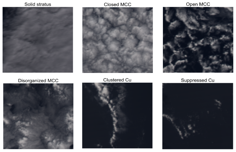
Figure 1 Example scenes of six cloud morphological types: solid stratus, closed mesoscale cellular convection, open mesoscale cellular convection, disorganized mesoscale cellular convection, clustered cumulus, and suppressed cumulus. These are visible light images composed of channels 1, 4, and 3, and the spatial resolution is 1° × 1°.

2.2 Data

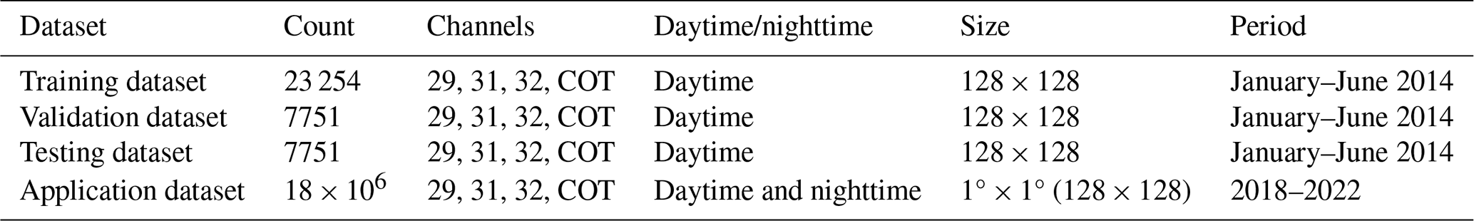
The primary observation data utilized in this study were derived from the Moderate Resolution Imaging Spectroradiometer (MODIS) aboard NASA's Aqua satellite, including the Level-1B radiance product MYD021KM and the Level-2 cloud product MYD06 (Platnick et al., 2017), both with a spatial resolution of 1 km at the nadir point. The thermal infrared radiance data from MYD021KM were used for model training and testing, while the cloud properties from MYD06 were utilized for quality control, low-cloud filtering, and statistical analyses. First, we selected daytime MODIS images over the south-eastern Pacific (SEP) from January to June 2014 to create our classification dataset. The representativeness of this dataset was validated because the probability density functions (PDFs) of thermal radiance data and cloud optical thickness show a large overlap with those of the global and full-year datasets (Fig. S1 in the Supplement). After dividing them into 128 × 128-pixel scenes, we filtered out the cloudless scenes (cloud fraction less than 1 %) and scenes containing a large number of high clouds or ice clouds (high or ice clouds exceeding 10 %). High clouds are defined as those with cloud-top heights above 6 km, and ice clouds are those with cloud-top temperatures below 273.15 K. In addition, severe stretching at the edges of MODIS granules has been avoided by filtering scenes with sensor zenith angles greater than 45°. Ultimately, these eligible scenes are manually classified into one of six categories. The cloud properties from the MYD06 product, such as cloud-top height (CTH), cloud liquid water path (CLWP), cloud optical thickness (COT), and cloud effective radius (CER), are used to help label and check the results with the cloud dataset (Mohrmann et al., 2021). A total of 38 756 labelled daytime scenes were obtained, including 3548 scenes of solid stratus, 6277 of closed MCC, 3345 of open MCC, 6739 of disorganized MCC, 8947 of clustered Cu, and 9900 of suppressed Cu. These scenes were then randomly partitioned into three mutually independent datasets for training, validation, and testing, with a distribution ratio of 3 : 1 : 1. Despite the disparity in sample sizes across the different types, our training dataset is capable of yielding superior model performance compared to a balanced dataset (Fig. S2).

In order to classify daytime and nighttime morphological types using one model only, we utilized daytime radiance data to train our model. Thermal infrared (TIR) channels 29 (8.7 µm), 31 (10.8 µm), and 32 (12.0 µm) were specifically chosen as they most effectively represent the cloud properties and cloud-top temperature. Notably, owing to the subtle temperature variations at the cloud top, our model is unable to comprehensively discern convective cellular structures within the clouds by using radiance data only. Incorporating COT can better address the model's shortcomings in studying these cellular structures by providing cloud thickness information. Considering that there is no nighttime COT in the Level-2 MYD06 cloud product, we used the COT data retrieved by Wang et al. (2022) as the fourth channel input for our model. Their all-day COT products, obtained using a TIR-CNN model, have shown good consistency with both daytime products from MODIS and all-day products from active sensors. To validate the reliability of using TIR-CNN-based COT as a replacement for MODIS COT, we conducted a sensitivity experiment comparing our classification with the outputs of a CNN trained on MODIS daytime COT. The results (Fig. S3) showed that the accuracy of both models is nearly identical, indicating that TIR-CNN-based COT is a reliable alternative to MODIS COT. In addition, we further examined the differences in the PDFs of the thermal radiance data and the TIR-CNN-based COT between our training dataset (daytime) and the nighttime dataset. As depicted in Fig. S4, these PDFs nearly overlapped, which means that less extrapolation will be introduced when the model is generalized to nighttime data. This also illustrates the credibility of our nighttime classification results. In summary, all the variables and datasets used in this study are outlined in Table 1.

Table 1 Summary of the datasets used in the study.

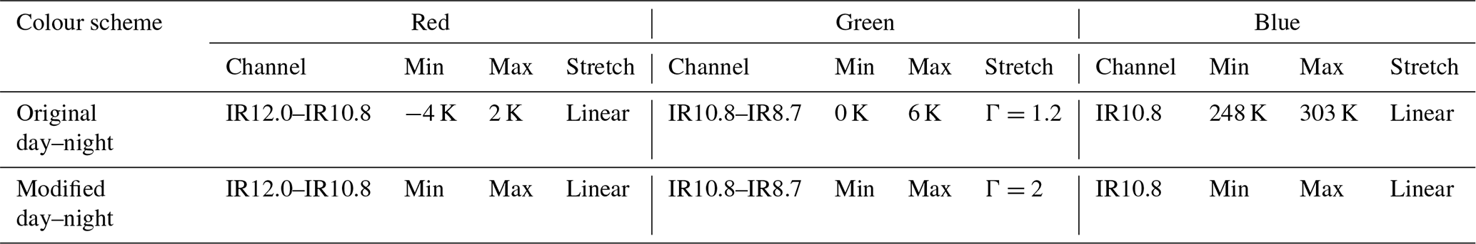
Before starting the training, we converted the radiance data into brightness temperature (BT) according to the inverse Planck function shown in Eq. (1):

$$\begin{array}{}\text{(1)}& \mathrm{BT}(\mathit{\lambda },L)={\displaystyle \frac{C_{\mathrm{2}}}{\mathit{\lambda }\ln (C_{\mathrm{1}}/{\mathit{\lambda }}^{\mathrm{5}}L+\mathrm{1})}},\end{array}$$

where λ is the wavelength (µm), L is the radiance (W m⁻² sr⁻¹ µm⁻¹), $C_{\mathrm{1}}=\mathrm{1.191042}\times {\mathrm{10}}^{\mathrm{8}}$ (W m⁻² sr⁻¹ µm⁴), and $C_{\mathrm{2}}=\mathrm{1.4387752}\times {\mathrm{10}}^{\mathrm{4}}$ (K µm). We combined BT data from the three thermal infrared channels according to the day–night colour scheme proposed by Lensky and Rosenfeld (2008) (Table 2). Table 2 includes both the original day–night colour scheme and our modified scheme used in this study. Different from the original day–night scheme, we did not clip each scene's data to a fixed range of maximum and minimum values. We think that clipping might lead to the loss of important information, such as convective cell characteristics, which will affect the model performance. In our scheme, the data of each scene may be compressed into different ranges and cause slight colour variations in each scene image (Fig. 4); this has little impact on the model's judgement capability since the convolutional neural network focuses primarily on the statistical relationships between adjacent pixels in satellite images (Goodfellow et al., 2016). Moreover, after multiple rounds of practical training adjustments, we decided to use a factor of 2 to stretch the green channel to achieve a better model prediction outcome. To enhance the training efficiency and accuracy, the combined BT data and COT are normalized using minimum–maximum normalization following Eq. (2):

$$\begin{array}{}\text{(2)}& x_{\mathrm{n}}={\displaystyle \frac{x-min\left(x\right)}{max\left(x\right)-min\left(x\right)}},\end{array}$$

where x represents the input data, x_n represents the data after normalization, and min(x) and max(x) represent the minimum and maximum values of the input data.

Table 2 The original (adapted from Lensky and Rosenfeld, 2008) and modified day–night colour schemes.

To align with conventional climate datasets, we developed a standard 1° × 1° gridded dataset by applying the trained model to 1° images, where the 1° × 1° satellite images were interpolated and refined to 128 × 128 pixels.

For the purpose of investigating the influence of meteorological conditions on low-cloud morphologies, we conducted some statistical analyses utilizing the co-located hourly ERA5 data (1° × 1°) from the European Centre for Medium-Range Weather Forecasts (ECMWF). The co-location is achieved by spatially selecting the ERA5 grid point nearest to each MODIS observation and temporally interpolating the ERA5 data to match the exact time of the MODIS observations. This ensures accurate alignment between the two datasets in both space and time. Several variables, such as sea surface temperature (SST), relative humidity (RH), vertical velocity (ω), and divergence (1000 and 700 hPa), can be obtained directly from the reanalysis data, while lower-tropospheric stability (LTS) needs to be calculated using the following Eq. (3):

$$\begin{array}{}\text{(3)}& \mathrm{LTS}={\mathit{\theta }}_{\mathrm{700}\mathrm{hPa}}-{\mathit{\theta }}_{\mathrm{1000}\mathrm{hPa}},\end{array}$$

where θ is the potential temperature.

Furthermore, we retrieved 5-year daytime and nighttime CER (r_e) and COT (τ) using the TIR-CNN model of Wang et al. (2022) for subsequent statistical analysis of cloud properties. This approach will ensure the consistency of data ranges by using the same cloud detection algorithm. We can further calculate the liquid water path (LWP) utilizing Eq. (4):

$$\begin{array}{}\text{(4)}& \mathrm{LWP}={\displaystyle \frac{\mathrm{2}}{\mathrm{3}}}{\mathit{\rho }}_{\mathrm{w}}\mathit{\tau }{r}_e,\end{array}$$

with ρ_w the density of liquid water.

2.3 Marine low-cloud mesoscale morphology dataset

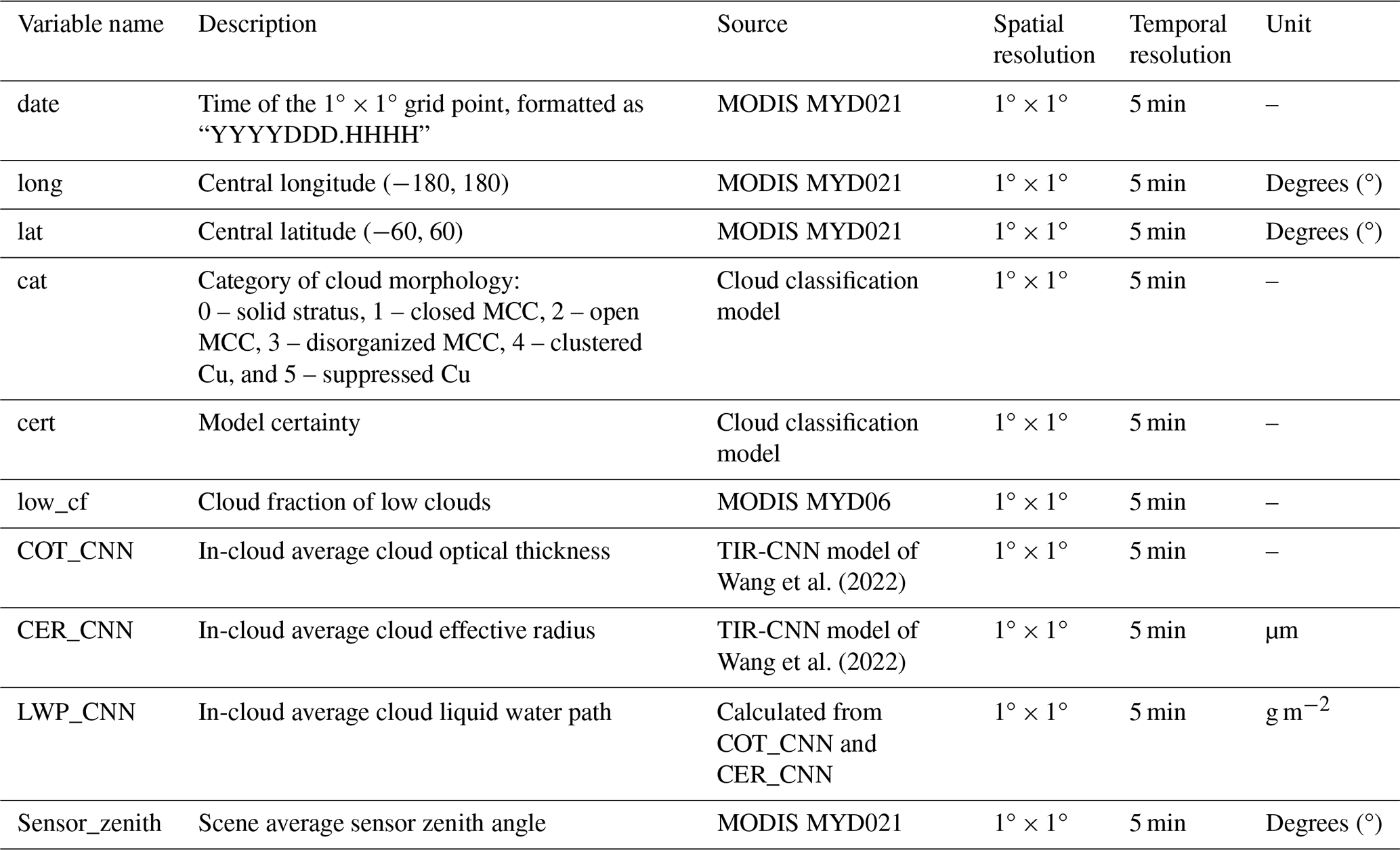
Our cloud dataset provides global classifications of daytime and nighttime marine low-cloud mesoscale morphology for the years 2018–2022, with a spatial resolution of 1° × 1° and a temporal resolution of 5 min. The dataset is provided in two kinds of files: those prefixed with “day” store the daytime classification results for each year, while files with the prefix “night” contain the nighttime classification results for each year. Both sets of files include the same variables. Table 3 provides an overview of the variables and their associated information. The key variables in the dataset include “date” (representing the time of the 1° × 1° scene, formatted as the MODIS granule date), “long” and “lat” (indicating the central longitude and latitude), and “cat” (the assigned cloud category, with the values 0 to 5 corresponding to “solid stratus”, “closed MCC”, “open MCC”, “disorganized MCC”, “clustered Cu”, and “suppressed Cu”, respectively). Additionally, “cert” represents the model certainty, quantifying the probability of the cloud morphology belonging to the assigned category. “low_cf” denotes the low cloud fraction, and “COT_CNN”, “CER_CNN”, and “LWP_CNN” denote the in-cloud average cloud optical thickness, effective radius, and liquid water path, respectively, as derived from the TIR-CNN model of Wang et al. (2022). The “Sensor_zenith” variable indicates the scene's average sensor zenith angle.

Table 3 Variables of the daytime and nighttime global marine low-cloud mesoscale morphology dataset.

2.4 Method

In this study, a machine learning (ML) model, ResNet50 (Koonce, 2021), was chosen as our model architecture. It is a deep CNN model which employs a residual learning framework to construct a network with 50 convolutional layers. Despite a fairly deep convolutional layer, the incorporation of residual units in ResNet50 enables direct signal transmission from earlier to later layers, ensuring high computational efficiency in deep architectures and markedly boosting the accuracy and speed of convergence. We made some adjustments to the overall architecture of ResNet50 to better suit our datasets, and the fine-tuned model structure is presented in Fig. 2a. The number of input channels was set to four to include the additional COT channel. Then, we configured the output dimension of the final fully connected layer to six to produce a probability distribution over the six output classes for each scene via the softmax activation function. The internal structure of ResNet50 remains unchanged, consisting of a preprocessing layer, four stages, and a global average pooling. The preprocessing layer includes a convolutional layer, a batch normalization (BN) layer, a rectified linear unit (ReLU) activation function, and a max-pooling layer. Each stage contains several residual blocks and is joined by skip connections (Fig. 2b).

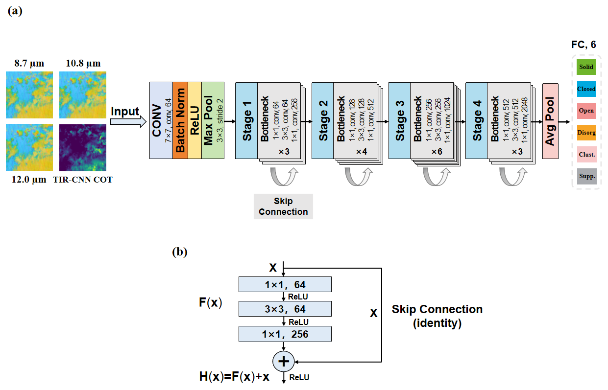
Figure 2 (a) The fine-tuned ResNet50 model architecture. (b) The skip connection structure of the residual blocks in the model.

Throughout the training process, we employed the Adaptive Moment Estimation (Adam) optimizer for gradient descent calculation and utilized cross-entropy as the loss function. Given the substantial size of our training dataset, we chose a batch size of 256 to enhance memory utilization and expedite the training process. In addition, to counteract the tendency to overfit due to the increased noise in the radiance data of thermal infrared channels, we applied random rotation augmentation to the training images with a 50 % probability. Lebesgue-2 (L2) regularization was also introduced to further decay the weights and prevent overfitting.

After each training epoch, the validation dataset was used to evaluate the trained model's performance, which allows us to monitor the model's success. When the training process was completed, the test dataset was used for the final evaluation of the model's performance. We used the optimal model to predict each sample in the test dataset, compared the model's predictions with the true labels, and assessed the accuracy using metrics such as accuracy, F1 score, and recall.

3 Results

3.1 Model performance

In this section, our model performance is evaluated and a nighttime classification example is given. Our model begins to show signs of convergence around the 50th epoch, with its maximum validation accuracy reaching around 92 % by the 65th epoch (Fig. S5). Compared to training without incorporation of COT, the model's accuracy improved by 4 %. Although this is a bit less accurate compared to the visible light model of Yuan et al. (2020), it is undeniable that this model has achieved a relatively high accuracy level when compared to other TIR models (Lang et al., 2022) and can effectively accomplish the classification tasks we proposed. The optimal model is subsequently evaluated on an independent test dataset, yielding the confusion matrix illustrated in Fig. 3. Elements on the diagonal represent the model's prediction accuracy for each type. Our model achieves an average precision of approximately 91 %, an F1 score of 90.6 %, and a recall of 90.8 % on the test dataset, demonstrating its strong generalization capability and robustness.

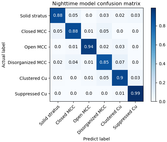
Figure 3 The confusion matrix of the model's predictions in the test dataset. The rows of the confusion matrix represent actual categories, and the columns represent predicted categories. The elements on the diagonal indicate the proportion of samples correctly classified by the model in each category.

Meanwhile, the confusion matrix (Fig. 3) shows that the model's predictive performance varies across six cloud types, with higher accuracy for suppressed Cu and open MCC but lower accuracy for disorganized MCC. Notably, this pattern is independent of sample size (Fig. S2) and is more likely due to confusion with other cloud types, as disorganized MCC clouds are frequently misidentified as clustered Cu or closed MCC (Fig. 3). Some classification samples reveal that such misclassifications are particularly common in mixed and transitional scenes (Fig. S6), where the overlapping features of different cloud types often lead to ambiguity in model predictions. In addition, considering the similarity between the morphologies of these clouds, the misclassifications may be related to the model's limited capacity to distinguish between stratiform structures and convective cells due to the small temperature difference at the cloud top. This can also be reflected in the sample images (Fig. S7).

Trained by daytime infrared data, this model can be applied to nighttime scenarios, as shown in Fig. 4. Circles with different colours represent different cloud categories within the 1° × 1° grid. Grids without circles indicate that they do not meet the criteria outlined in Sect. 2. The pseudo-RGB images are composed of thermal infrared channels 29, 31, and 32, following the modified day–night colour scheme (Table 2). This scheme makes a clearer visual distinction between the different cloud types. However, as the data range for each image is not fixed, the colours of the different cloud types will vary in different situations. For example, in the left granule image, light yellow represents low water clouds, green indicates thin cirrus, and dark yellow signifies thick cumulonimbus clouds. In the sample scenes of open MCC and suppressed Cu, the yellow of the low clouds becomes lighter and the green indicates small cumulus clouds. As for the four remaining cloud types, the surrounding thin cirrus appears in green, while the stratiform clouds and shallow cumulus convections are both depicted in a brighter yellow due to their similar temperatures. Thus, it is challenging to discern convective cells in the yellow background of stratiform clouds. That is why we incorporated COT, in order to assist in the model predictions.

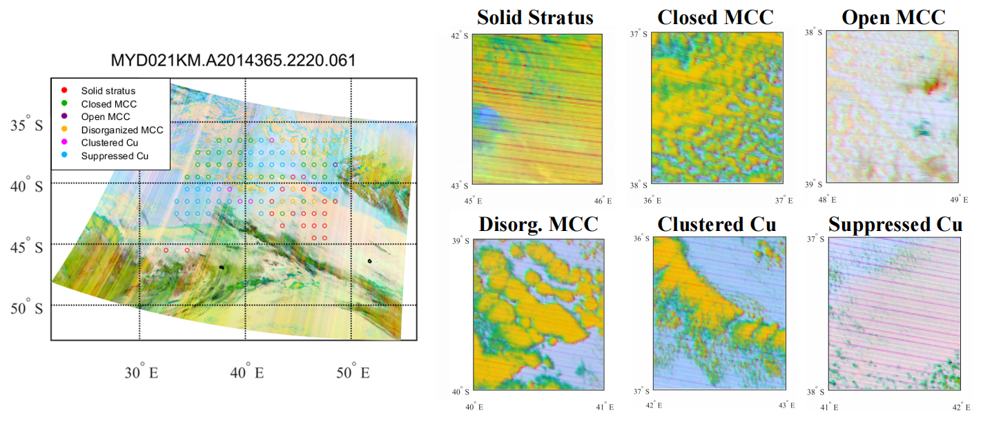
Figure 4 A nighttime classification example of a MODIS image, taken at 22:20 UTC on 31 December 2014. The pseudo-RGB images were generated from the combination of 29, 31, and 32 thermal infrared channels, while the classification results were derived by incorporating the retrieved cloud optical thickness (COT) data.

3.2 Climatology of the morphological types

Using the well-trained ResNet50 model, we classified nearly 18 million 1° MODIS scenes and recorded the occurrence counts of different cloud types. The occurrence counts of each cloud type were divided by the total occurrences of the six cloud types within each grid to calculate their relative frequency of occurrence (RFO). The daytime climatology of the RFOs for the six cloud types is presented in Fig. 5. Each subplot's upper-right corner displays n and a percentage, with n denoting the total number of occurrences for each cloud type during daytime over the 5-year period, while the percentage indicates the proportion of each cloud type's 5-year occurrences (n) relative to the 5-year total occurrences of all six cloud types, which is called the total relative frequency.

Solid stratus is predominantly distributed in nearly symmetrical latitude bands between 40–60° N and 50–60° S with a total relative frequency of 14 %. At the middle to high latitudes of the Southern Hemisphere, its RFO exceeds 90 %, which is higher than that of the Northern Hemisphere. Additionally, a substantial presence of solid stratus is observed along the western coasts of the continents in tropical and subtropical regions. Closed MCCs mainly appear in the cold eastern subtropical and mid-latitude oceans, with marked peaks along the western coasts of North America, South America, and Africa. Their total relative frequency during the daytime is relatively low, accounting for only 5 %. Disorganized MCC exhibits a distribution pattern similar to that of closed MCC but is typically located farther offshore. It covers a more extensive area and occurs more frequently. The total relative frequency of disorganized MCC during the daytime is 15 %, which is 3 times higher than that of closed MCC. In addition, it is worth noting that the peak areas of disorganized MCC appear to the west of closed MCC. This may be related to the transition between these two cloud types. The occurrence of open MCC is least frequent over the global ocean, accounting for only 3 %. In the water areas west of Peru, there is a minor frequency peak of open MCC, which may be due to the fragmentation of closed MCC caused by strong winds and precipitation (Rosenfeld et al., 2006; Eastman et al., 2022). Clustered Cu and suppressed Cu are primarily observed in tropical and subtropical regions. They have the highest overall relative frequencies; both are around 30 %. However, in terms of its spatial distribution, clustered cumulus is more prevalent over the central and western oceans, while suppressed Cu commonly peaks in coastal waters near the continents. We have compared the daytime climatology with the results of Yuan et al. (2020) using visible light channels, and consistent results were obtained (Fig. S8).

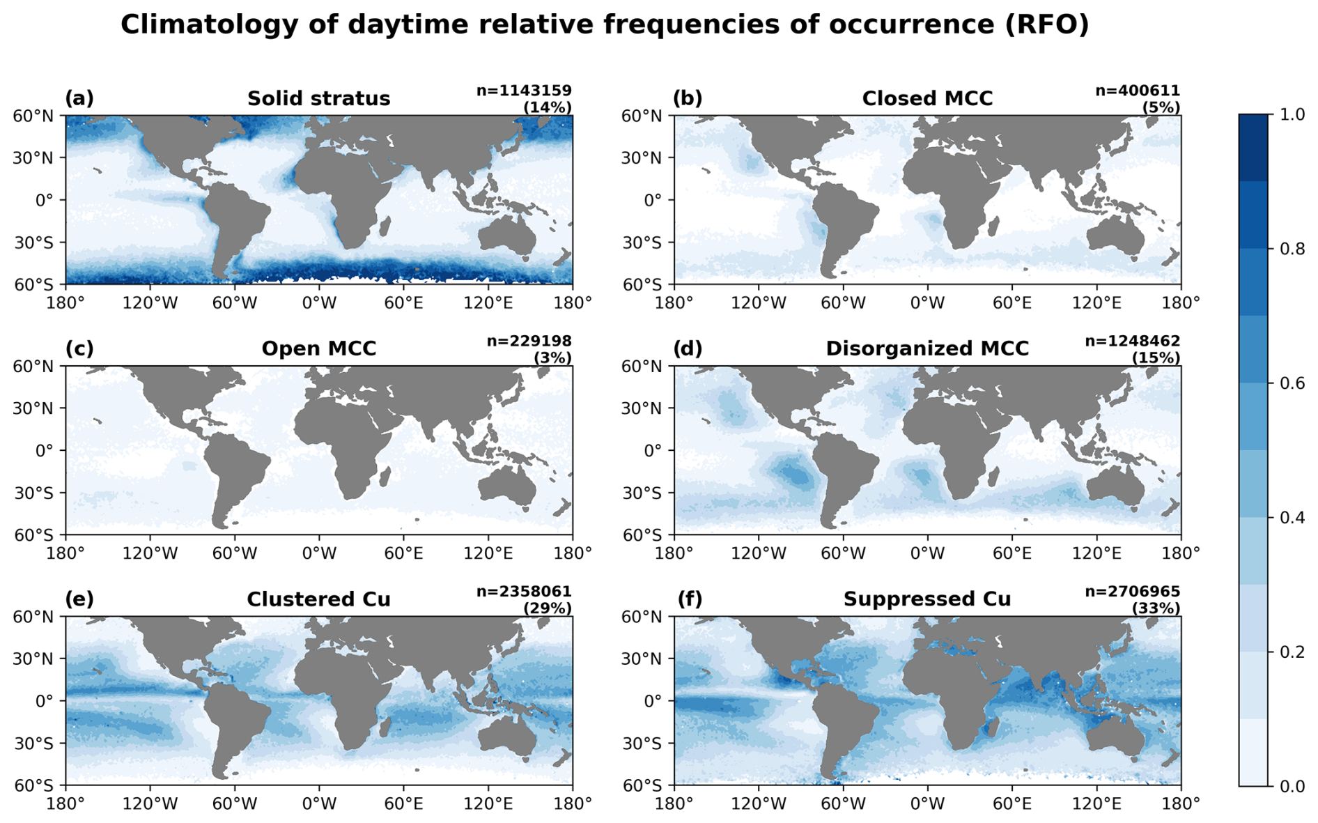
Figure 5 The climatology of the daytime relative frequencies of occurrence (RFOs) for the six categories from 2018 to 2022. N represents the total number of occurrences for each cloud type during the day over the 5-year period, while the percentage indicates the proportion of each cloud type's 5-year occurrences relative to the total number of 5-year occurrences of all six cloud types.

In Fig. 6, the spatial distribution of these six cloud types remains largely unchanged at night, but their RFOs show notable variations. Figure 7 presents the nighttime–daytime contrast in RFOs for each morphological type (nighttime minus daytime). The total nocturnal frequency of solid stratus clouds is 15 %, which is similar to daytime. At night, they occur more frequently over mid-latitude oceans and less frequently in low-latitude regions. The RFO for closed MCC shows a pronounced increase at night, reaching approximately twice the levels of the day. Some of the increase occurs over mid-latitude oceans, while the most significant rise is observed over the eastern subtropical ocean, particularly in the Southern Hemisphere (Fig. 7). The overall frequency of open MCC remains relatively unchanged at night, while the total frequencies of disorganized MCC and clustered Cu increase slightly. At night, the RFOs of all three cloud types decrease over the colder eastern subtropical and mid-latitude oceans and increase over the warmer sea surface at lower latitudes (Fig. 7). Notably, west of the continents, the nighttime frequency pattern of disorganized MCC exhibits an initial decrease, followed by an increase. This opposite trend is most pronounced along the western coast of South America. Of the six cloud types, only the total frequency of suppressed Cu experiences a marked decline at night, with a total decrease of 11 %. A statistical analysis of some meteorological conditions will be conducted in Sect. 3.5. Exploration of the critical cloud-controlling factors contributing to these diurnal variations will be made in the future.

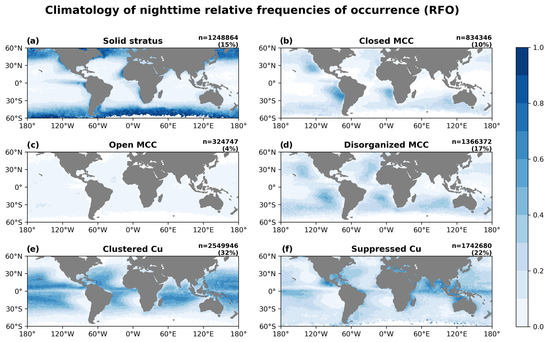
Figure 6 The climatology of the nighttime RFOs for the six categories from 2018 to 2022.

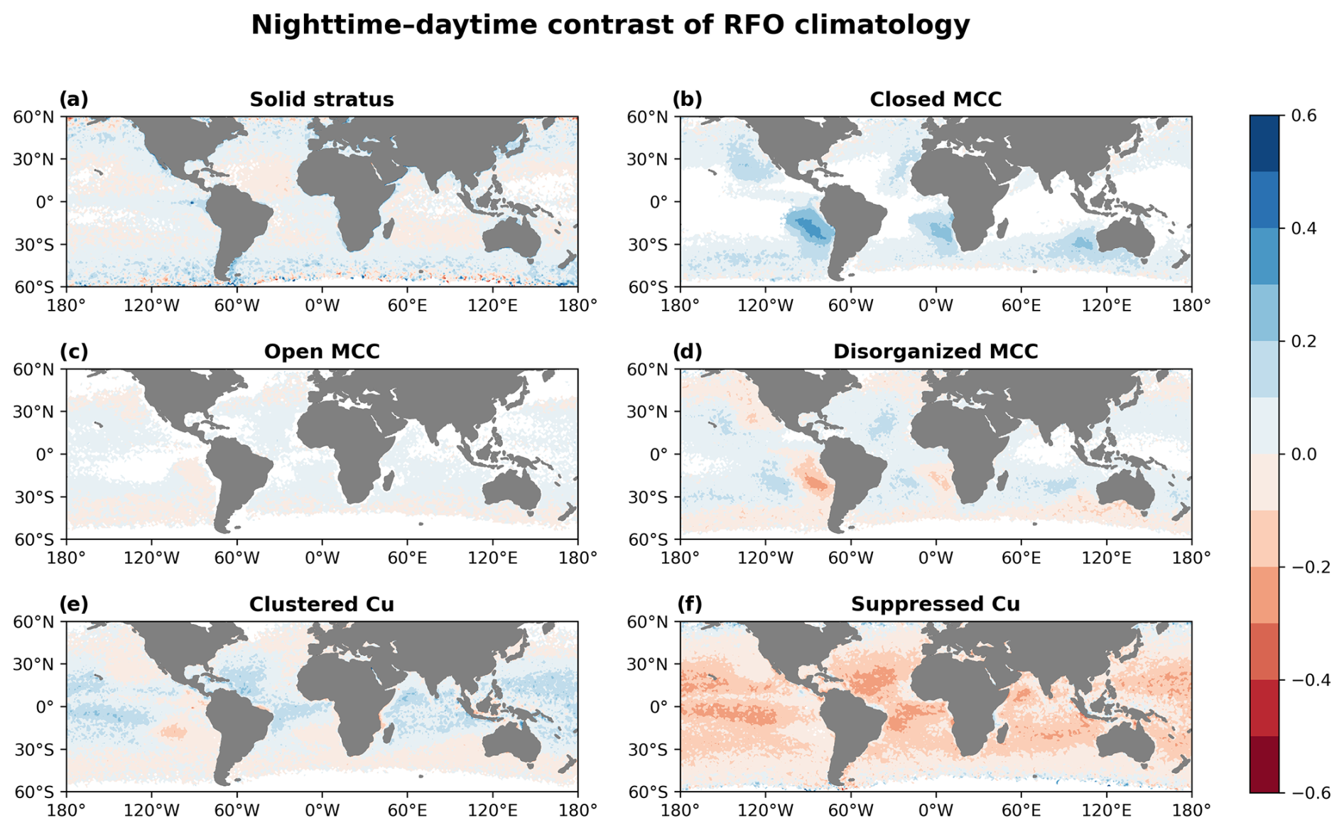
Figure 7 The difference between the daytime and nighttime RFOs for each morphological type (nighttime minus daytime).

3.3 Seasonal variations in morphological types

We further classified the RFOs of different cloud morphologies by season. Figure 8 presents the seasonal variation of daytime RFOs, while Fig. 9 shows the nighttime situation. It can be seen from the two figures that the RFOs of these six cloud types exhibit similar seasonality during both daytime and nighttime. At middle latitudes, solid stratus clouds usually peak during the summer of the respective hemisphere (June–July–August (JJA) for the Northern Hemisphere and December–January–February (DJF) for the Southern Hemisphere) and have the lowest occurrence during winter (DJF for the Northern Hemisphere and JJA for the Southern Hemisphere). They show equal RFOs during spring and autumn in both hemispheres (March–April–May, MAM, and September–October–November, SON). The peak occurrence of solid stratus in mid-latitude regions aligns with the latitudinal shift in solar insolation. Thus, it can be inferred that the increased temperature and enhanced moisture available from melted sea ice may contribute to the peak in summer (Herman and Goody, 1976). The RFO of closed MCC notably increases during winter (JJA) and spring (SON) in the Southern Hemisphere, particularly in the SEP and south-eastern Atlantic (SEA) regions. McCoy et al. (2017) suggested that the seasonal cycle of closed MCC in such regions correlates well with the estimated inversion strength (EIS). In contrast to solid stratus, open MCC demonstrates an opposite seasonal cycle at the middle latitudes, with the highest frequency occurring in the winter of the respective hemisphere (DJF for the Northern Hemisphere and JJA for the Southern Hemisphere). Previous work suggests that its seasonality is more likely associated with cold-air outbreaks in mid-latitude oceanic regions (McCoy et al., 2017). This may also explain why open MCC exhibits a zonal frequency peak over the South Pacific during the winter of the Southern Hemisphere (JJA) (Figs. 8 and 9). Disorganized MCC clouds occur more frequently over warmer ocean surfaces west of the continents during the summer of the respective hemisphere (JJA in the Northern Hemisphere and DJF in the Southern Hemisphere) and occur less frequently during the winter of the respective hemisphere (DJF in the Northern Hemisphere and JJA in the Southern Hemisphere). Thus, the sea surface temperature may be one of the controlling factors of its seasonal variation. All of the MCC types show distinct seasonal cycles, while the clustered Cu and suppressed Cu do not show marked seasonal variations during both daytime and nighttime.

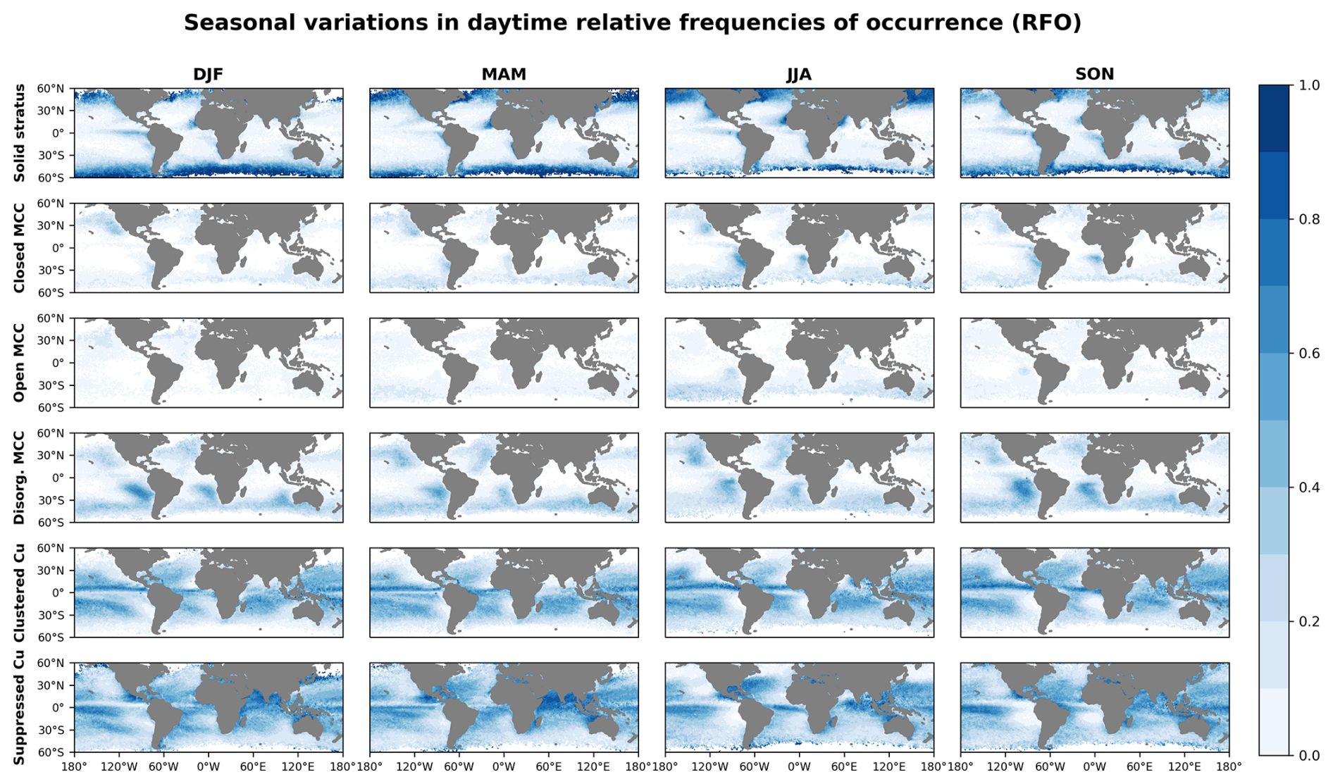
Figure 8 Seasonal variations of the daytime RFOs.

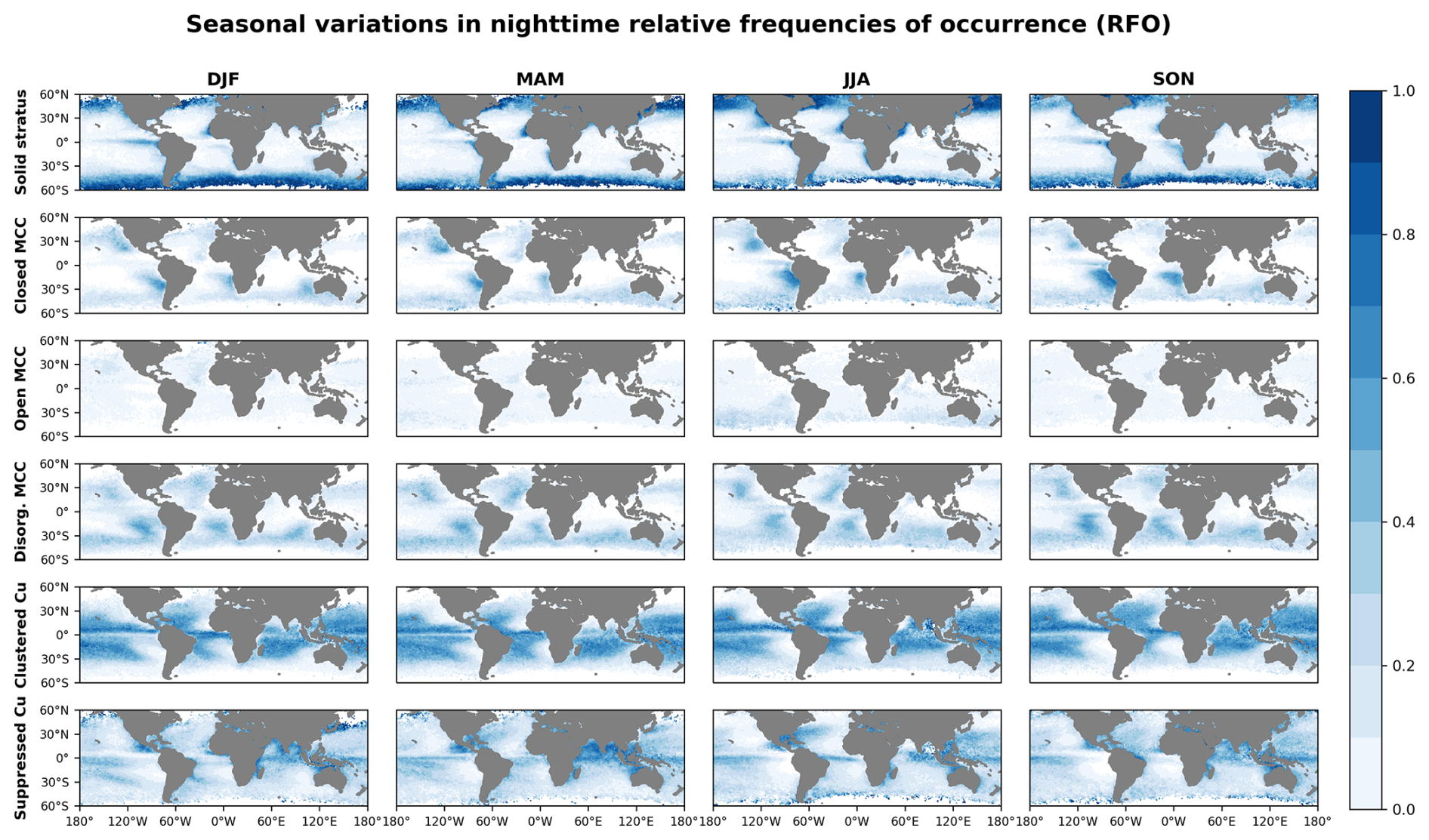
Figure 9 Seasonal variations of the nighttime RFOs.

3.4 Cloud properties

Different cloud types exhibit different radiative effects due to their unique physical characteristics. In Fig. 10, we compared the physical properties of each cloud type during both the day and the night, including cloud fraction (CF), CER, cloud LWP, and COT. The CF is derived from the cloud mask in the Level-2 cloud product MYD06, while CER and COT are both retrieved using the method of Wang et al. (2022). LWP is calculated from CER and COT, as mentioned in Sect. 2.2. All of the cloud microphysical properties represent the in-cloud mean value within a 1° × 1° grid.

Solid stratus and closed MCC possess the highest CF, and therefore the increase in their nocturnal frequency may account for a major portion of the overall rise in cloud cover. Open MCC possesses the largest CER, and it will decrease by 2 µm on average at night. During the day, closed MCC clouds exhibit the highest values of LWP and COT. At night, their CER, LWP, and COT increase further substantially, with a substantial magnitude. The four cloud properties of disorganized MCC also show a slight increase at night.

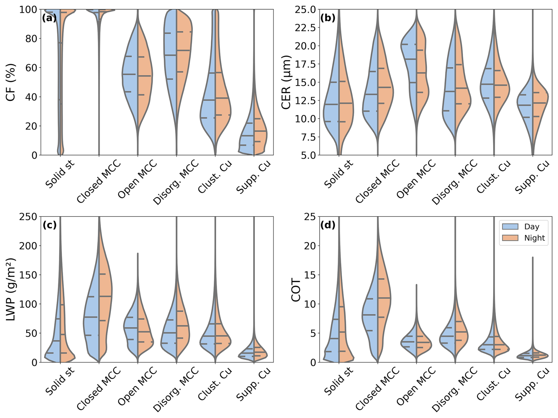
Figure 10 A violin plot of the properties of the six cloud types over the global oceans from 2018 to 2022. (a) Cloud fraction, (b) retrieved cloud effective radius, (c) cloud liquid water path, and (d) retrieved cloud optical thickness. Blue represents the daytime data and yellow represents the nighttime data. The central long dashed line in each plot represents the median of the distribution, and the short dashed line represents the interquartile range. The shape of the violin plots suggests the density distribution of the values, with wider sections indicating a higher frequency of data points.

3.5 Large-scale meteorological condition

The statistics of several meteorological factors which may control the marine low-cloud morphology in the SEP region (0–30° S, 80–120° W) are shown in Fig. 11. The LTS for the six cloud types is shown in Fig. 11a. A higher LTS indicates a more stable lower troposphere. Closed MCC has the highest LTS, implying the significance of tropospheric stability in its formation. The two cumulus types have the lowest LTS because an unstable troposphere is conducive to cumulus activity. The LTS of the six cloud types shows different degrees of decline at night, which may be due to the shift in their geographical locations. SST is lowest for closed MCC during both the day and the night (Fig. 11b). Open MCC and disorganized MCC exhibit higher SST compared with closed MCC, which corresponds to their geographical positions. The two cumulus types have the highest SST. At night, the increase in SST for the different cloud types may also be attributed to their movements. Figure 11c and d show the RH at 700 and 1000 hPa, respectively. Throughout the day and night, solid stratus clouds exhibit the highest RH at both 700 and 1000 hPa. At the 700 hPa level (Fig. 11c), the RH values for the two cumulus types are higher than those for MCC clouds, while at the 1000 hPa level (Fig. 11d) the difference is minimal. At night and at 700 hPa, the RH of solid stratus and the two cumulus types increases, while that of closed MCC decreases. Due to lower temperatures at night, the RH over the sea surface for all six cloud types increases by a similar magnitude. Figure 11e indicates that all of the cloud types are associated with large-scale subsidence. Open MCC experiences the strongest upper-level subsidence, while solid stratus has the weakest vertical motion. At night, the subsidence for all six cloud types weakens and closed MCC exhibits a more pronounced reduction. Figure 11f presents the boundary layer anomaly divergence, which is calculated by subtracting the divergence at 700 hPa from the surface divergence. This index has been proven to be effective in distinguishing between the two cumulus types (Mohrmann et al., 2021). Suppressed Cu shows the largest boundary layer anomaly divergence, indicating that strong surface divergence favours the maintenance of suppressed Cu. Clustered Cu has the smallest anomaly divergence, with weaker surface divergence. Therefore, the weakening of surface divergence at night may be the reason for the reduction of suppressed Cu.

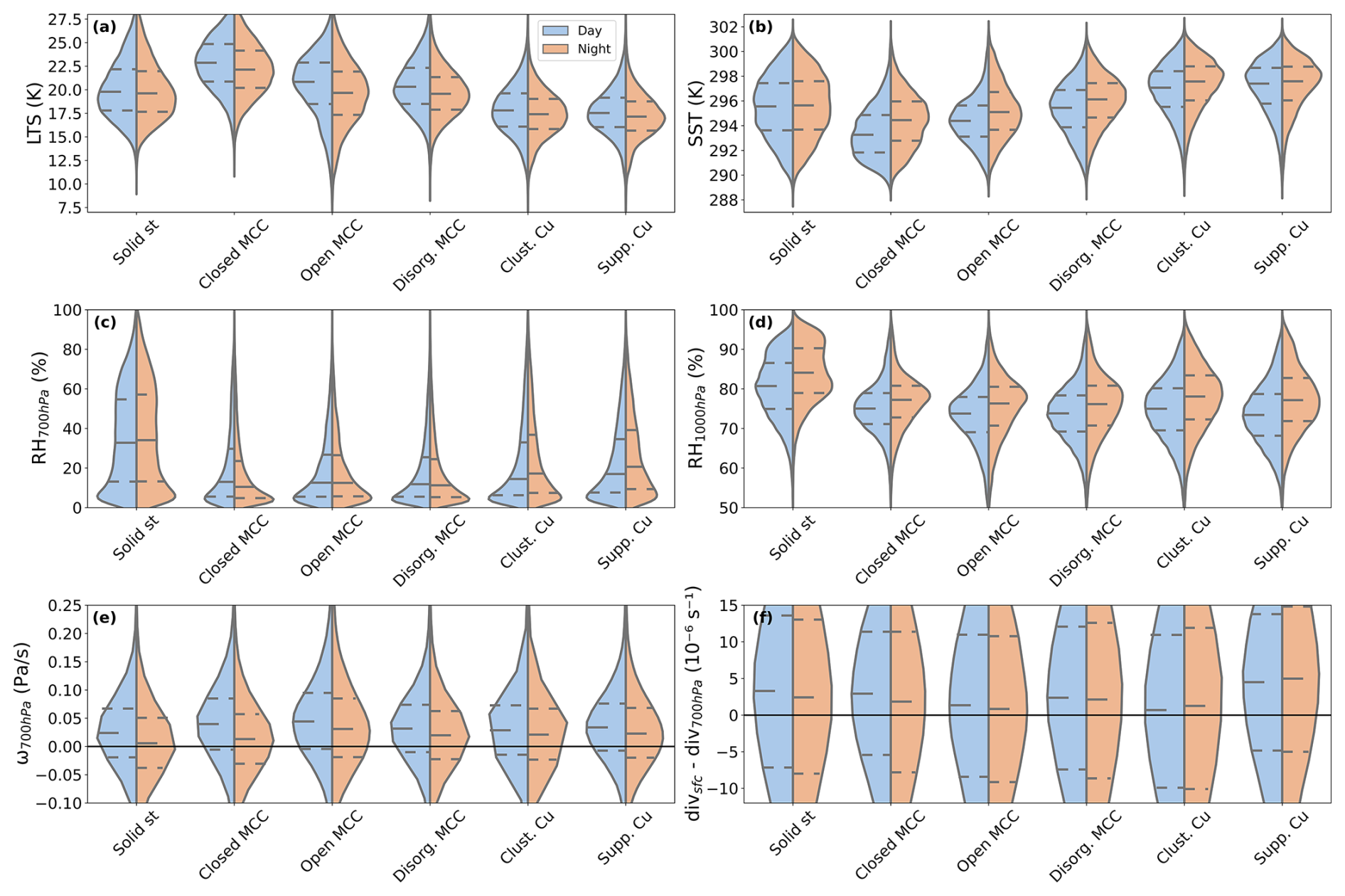
Figure 11 Same as Fig. 10 but showing a day–night comparison of meteorological conditions in the south-eastern Pacific (SEP) region (0–30° S, 80–120° W) from 2018 to 2022. This is matched from ERA5 data. (a) Lower-tropospheric stability, (b) sea surface temperature, (c) 700 hPa relative humidity, (d) 1000 hPa relative humidity, (e) 700 hPa vertical velocity, and (f) boundary layer anomaly divergence.

4 Discussion

The mesoscale cloud morphology dataset presented in this paper enables a comparative investigation of cloud morphology during both daytime and nighttime. Its 1° × 1° resolution allows better alignment with other gridded datasets, facilitating further studies on driving factors, precipitation efficiency, and radiative effects (shortwave and longwave).

Although our model achieved a high prediction accuracy and performed well in the classification tasks, there is still room for improvement. In future work, the current CNN model might be replaced with more advanced architectures and the quality of our training dataset could be improved further. For the former, novel deep CNN models can be applied to cloud morphology classification through transfer learning. For instance, the Xception model, which achieved an accuracy of 97.66 % in classifying traditional cloud types (Guzel et al., 2024), could be considered. For the latter, removing the mixed and mislabelled scenes from our training dataset and adding more global and multi-seasonal scenes will improve the model performance in identifying these cloud morphological types. Furthermore, the limitations of brightness temperature in capturing cloud-top morphology significantly constrain the model's accuracy, which largely explains the performance gap between our nighttime model and the daytime model proposed by Yuan et al. (2020). Nevertheless, a 4 % improvement in model accuracy achieved by incorporating COT indicates that integrating additional cloud property channels represents a promising avenue for further enhancement of the performance of our model.

As we apply the model trained on 128 × 128-pixel scenes to the interpolated 1° × 1° cloud scenes, the issue of scene area requires further discussion. For a given latitude, when the satellite zenith angle changes, the area of 128 × 128 pixels will vary due to the pixel stretching, while the area of the 1° grid remains constant. This is an advantage of the 1° × 1° grid dataset, as a larger area has a larger possibility of covering multiple cloud types in one scene. However, at the same satellite zenith angle, the size of the 1° × 1° grid will change with latitude, whereas the 128 × 128-pixel scene area remains undistorted, which is a limitation of the 1° × 1° grid dataset. Moreover, in some cases, and especially with stratocumulus and cumulus clouds, interpolating images into a 1° × 1° grid may smooth or blur small-scale cloud features and introduce unrealistic structures that do not exist in the original images, which could lead to potential misclassifications of the model. Therefore, testing the model on a labelled standard-grid dataset will be necessary in future work.

The six cloud types examined in this study are the most common and representative types over the ocean. However, they are not exhaustive. In future work, we will explore all low-cloud morphological types over the global land and ocean and gradually extend this to mid- and high-level clouds.

5 Code and data availability

The daytime and nighttime cloud classification datasets, along with the model development datasets (training, validation, and test datasets), are accessible at https://doi.org/10.5281/zenodo.13801408 (Wu et al., 2024). The model and code related to this article are available at https://doi.org/10.5281/zenodo.15776240 (Wu et al., 2025). The MODIS data can be downloaded from NASA's official website (https://ladsweb.modaps.eosdis.nasa.gov/, LAADS, 2025). The ERA5 data are provided by ECMWF (https://cds.climate.copernicus.eu/datasets, Climate Data Store, 2025). The cloud property retrieval model of Wang et al. (2022) can be found at https://github.com/WgQuan/cloud-property-retrievals.

6 Conclusion

In this study, approximately 40 000 MODIS daytime low-cloud scenes were labelled manually to train a deep residual network model (ResNet50). By using this model, we developed a new global standard-grid classification dataset (2018–2022) of marine low-cloud mesoscale morphology, encompassing classifications for both daytime and nighttime. Compared to the 128 × 128-pixel dataset of Yuan et al. (2020) and Mohrmann et al. (2021), our standard-grid dataset offers more uniform and widely applicable cloud morphology data and, more importantly, extends the dataset to nighttime. This dataset can integrate more easily with other climate and surface datasets and thus will provide a solid data foundation for future research on understanding cloud dynamics and their impact on the climate.

The climatology of cloud morphologies is also analysed. The results reveal that solid stratus dominates within the 50–60° latitude bands and that closed MCC is most commonly found in the cold eastern subtropical and mid-latitude oceans. Disorganized MCC occurs on the warmer ocean surfaces west of closed MCC, with a much higher frequency. Open MCC is more evenly distributed across the global oceans but with the lowest frequency. In regions with higher sea surface temperatures, such as the tropics and the trade wind zone, clustered Cu and suppressed Cu are the primary types of marine low clouds. Clustered Cu is more prevalent over oceans and suppressed Cu is more concentrated along continental coasts.

When comparing the daytime and nighttime climatologies, we found that there was a pronounced increase in the RFO of closed MCC at night, whereas the occurrence of suppressed Cu undergoes a significant decline. The frequencies of disorganized MCC and clustered Cu exhibit a minor variation between day and night. From the perspective of different seasons, solid stratus and all MCC types exhibit clear seasonal cycles, while the two cumulus types do not show notable seasonality.

Although we have statistically analysed the meteorological factors that may affect low-cloud morphology, identifying the specific dominant factors in each cloud type remains challenging. In the context of global warming, the long-term trends of these cloud types during daytime and nighttime may also exhibit significant differences. The changes in Earth's radiation budget caused by low-cloud morphology transitions may have a substantial impact on climate sensitivity, which will be a topic of our future research.