Mapping the world's inland surface waters: an upgrade to the Global Lakes and Wetlands Database (GLWD v2)

In recognition of the importance of inland waters, numerous datasets mapping their extents, types, or changes have been created using sources ranging from historical wetland maps to real-time satellite remote sensing. However, differences in definitions and methods have led to spatial and typological inconsistencies among individual data sources, confounding their complementary use and integration. The Global Lakes and Wetlands Database (GLWD), published in 2004, with its globally seamless depiction of 12 major vegetated and non-vegetated wetland classes at 1 km grid cell resolution, has emerged over the last few decades as a foundational reference map that has advanced research and conservation planning addressing freshwater biodiversity, ecosystem services, greenhouse gas emissions, land surface processes, hydrology, and human health. Here, we present a new iteration of this map, termed GLWD version 2, generated by harmonizing the latest ground- and satellite-based data products into one single database. Following the same design principle as its predecessor, GLWD v2 aims to avoid double counting of overlapping surface water features while differentiating between natural and non-natural lakes, rivers of multiple sizes, and several other wetland types. The classification of GLWD v2 incorporates information on seasonality (i.e., permanent vs. intermittent vs. ephemeral); inundation vs. saturation (i.e., flooding vs. waterlogged soils), vegetation cover (e.g., forested swamps vs. non-forested marshes), salinity (e.g., salt pans), natural vs. non-natural origins (e.g., rice paddies), and stratification of landscape position and water source (e.g., riverine, lacustrine, palustrine, coastal/marine). GLWD v2 represents 33 wetland classes and – including all intermittent classes – depicts a maximum of 18.2 ×10⁶ km² of wetlands (13.4 % of the global land area excluding Antarctica). The spatial extent of each class is provided as the fractional coverage within each grid cell at a resolution of 15 arcsec (approximately 500 m at the Equator), with cell fractions derived from input data at resolutions as small as 10 m. The upgraded GLWD v2 offers an improved representation of inland surface water extents and their classification for contemporary conditions (∼ 1984–2020). Despite being a static map, it includes classes that denote intrinsic temporal dynamics. GLWD v2 is designed to facilitate large-scale hydrological, ecological, biogeochemical, and conservation applications, aiming to support the study and protection of wetland ecosystems around the world. The GLWD v2 database is available at https://doi.org/10.6084/m9.figshare.28519994 (Lehner et al., 2025).

1 Introduction

Wetland ecosystems ranging from lakes and rivers to marshes, swamps, peatlands, mangroves, and numerous other wetland types are critically important for humans and Earth system processes. As key components of global hydrological and biogeochemical cycles and as habitats for biodiversity, they provide some of the most valuable ecosystem services to human society (Costanza et al., 1998; Millennium Ecosystem Assessment, 2005). Wetlands directly and indirectly influence many environmental and socio-economic systems through their carbon storage (e.g., Chmura et al., 2003; Duarte et al., 2005; Raymond et al., 2013; Hugelius et al., 2020); nutrient processing (e.g., Cheng et al., 2020); provision of water, food, and other resources (e.g., Mitsch et al., 2015); biological productivity (e.g., Gibbs, 2000; Mitchell, 2013); flood and drought mitigation (e.g., Tallaksen and van Lanen, 2004; Čížková et al., 2013; Junk et al., 2013); coastal protection (e.g., Gedan et al., 2011; Marois and Mitsch, 2015); and water quality regulation (e.g., Verhoeven and Setter, 2010).

Accurate and comprehensive maps of wetland ecosystems are fundamental to quantifying their role within the water, carbon, and nutrient cycles; to planning conservation and restoration actions; to guiding effective resources management; and to assessing and mediating human interactions and pressures (van Asselen et al., 2013; Qiu et al., 2021). Beyond knowledge of their areal extent, characteristics such as vegetation, hydrology, salinity, and connectivity are critical for distinguishing the roles and behaviors of different wetland types. As a critical input to hydrologic and Earth system models, global lake and wetland distributions are of particular interest for current and future water resource assessments, carbon and nutrient budget calculations, climate change projections, and other large-scale land surface studies (e.g., Bullock and Acreman, 2003; Lauerwald et al., 2023). Consistent information across large scales is required to set a global baseline to contextualize long-term degradation of wetland ecosystems (Vörösmarty et al., 2010; Darrah et al., 2019; Murray et al., 2019) and forecasted risks from environmental change (e.g., Xi et al., 2021), as well as to offer interim data to countries currently lacking (or having outdated) national inventories (Davidson et al., 2018). While freshwater biodiversity is among the most threatened in the world (Ramsar Convention on Wetlands, 2021), several regions or countries have nearly eradicated their wetland cover since pre-industrial times (Fluet-Chouinard et al., 2023). Reliable maps are therefore needed for monitoring the progress towards global conservation targets, such as to track changes in the extent of water-related ecosystems over time as mandated by the United Nations Sustainable Development Goal 6.6 (to protect and restore water-related ecosystems, including mountains, forests, wetlands, rivers, aquifers and lakes).

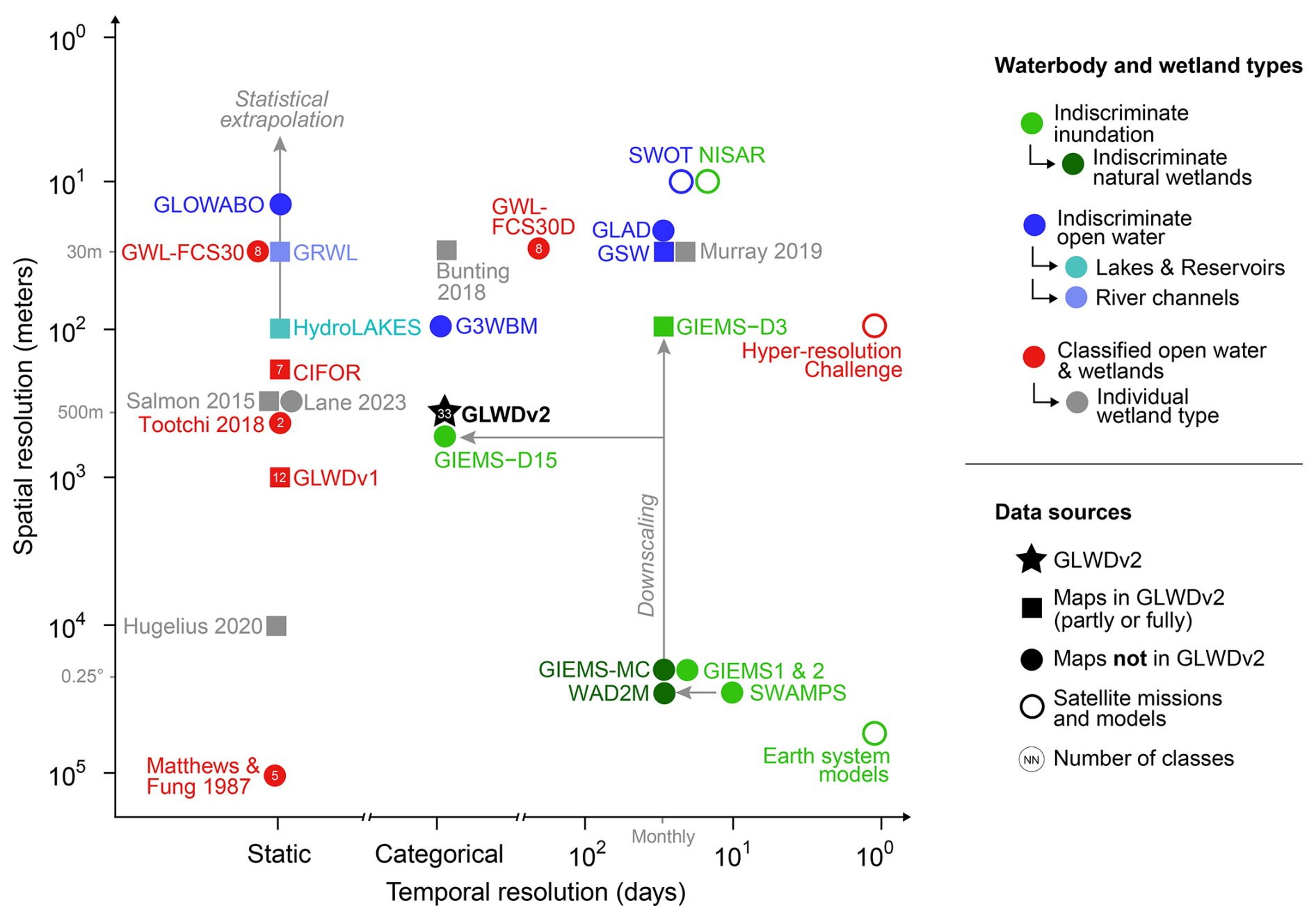
Figure 1 Common surface water datasets plotted according to their spatial and temporal resolution. Only maps with global or near-global extent, covering >80° of latitudinal swaths, are included. The colors of points represent the typological level of each dataset and together illustrate that classified maps including multiple wetlands and waterbody types have largely remained at a coarser resolution than available data products of indiscriminate wetland types. Arrows in the plot represent which datasets have been used in the production of others. Square points represent data products that were included in the creation of GLWD v2 as presented in this paper (additional detail on these sources can be found in Table 1). The spatial resolution is in meters at the Equator. Data products listed as static do not contain information on inundation frequency, while data products depicting hydrological regimes with qualitative measures are labeled as categorical. Explanations of dataset abbreviations and brief descriptions of each dataset's main characteristics are provided in Table A1 (Appendix A). References for data sources are as follows: G3WBM – Yamazaki et al. (2015), GIEMS-1 – Prigent et al. (2007), GIEMS-2 – Prigent et al. (2020), GIEMS-D3 – Aires et al. (2017), GIEMS-D15 – Fluet-Chouinard et al. (2015), GIEMS-MC – Bernard et al. (2024), GLAD – Pickens et al. (2020), GLOWABO – Verpoorter et al. (2014), GLWD v1 – Lehner and Döll (2004), GRWL – Allen and Pavelsky (2018), GSW – Pekel et al. (2016), GWL_FCS30 – Zhang et al. (2023), GWL_FCS30D – Zhang et al. (2024), HydroLAKES – Messager et al. (2016), SWAMPS – Jensen and McDonald (2019), and WAD2M – Zhang et al. (2021).

Global maps of inland (non-marine) wetland ecosystems have improved continuously over the last 4 decades (Fig. 1). Literature estimates of global wetland extents range broadly from 5 ×10⁶ to 13 ×10⁶ km², with lower and upper boundaries of 2 ×10⁶ and 17 ×10⁶ km² (Lieth, 1975; Matthews and Fung, 1987; Aselmann and Crutzen, 1989; Dugan, 1993; Finlayson and Davidson, 1999; Spiers, 1999, 2001; Lehner and Döll, 2004; Prigent et al., 2007; Tiner, 2009; Fluet-Chouinard et al., 2015; Mitsch and Gosselink, 2015; Zhang et al., 2023). The wide range is explained by differences in data sources, methodologies, and definitions. Early wetland estimates inherited gaps and inconsistencies from the compilation of national or regional inventories, limiting the reliability of their global perspective (Nivet and Frazier, 2004; Davidson et al., 2018). Over time, compilations of paper maps were replaced by satellite remote sensing imagery and its interpretation using machine learning and artificial intelligence, which allowed for seamless mapping across the world at shorter time intervals (Gallant, 2015). These improvements in methods coincided with an increase in the global area of wetland ecosystems mapped over time (Davidson et al., 2018). Nonetheless, wetlands remain the land cover class with the least agreement when comparing across global data products, in which wetlands are often being misclassified as forest, shrub, cropland, or grassland (Nakaegawa, 2012). Even advanced remote sensing methodologies and sensors face challenges in detecting different wetland types or delineating the hydrologically active extent of wetlands, for example, when cloud or vegetation cover obstructs the view or when saturated soils are confused with surface inundation (Gallant, 2015). Besides restrictions in spatial and/or temporal resolution, remote sensing approaches are also constrained by their limited historical extent as the first missions launched only in the 1970s.

Differences in definitions of what constitutes an aquatic ecosystem or wetland are the primary factor impeding comparisons across estimates and data sources. The Ramsar Convention on Wetlands (1971) adopted a broad definition of wetlands, comprising nearly all types of aquatic ecosystems as “areas of marsh, fen, peatland or water, whether natural or artificial, permanent or temporary, with water that is static or flowing, fresh, brackish, or salt, including areas of marine water the depth of which at low tide does not exceed six meters.” However, this definition is not universally accepted (Gerbeaux et al., 2018), and wetland criteria designed for field use are not practical for broad-scale mapping as shown by the wide range of areal estimates across studies (Mahdavi et al., 2018). Individual global map products typically provide their own, narrower definitions justified by methodological limitations. For instance, inundation maps from passive microwave sensors may omit non-inundated peatlands and may require post-processing to exclude coastal and/or offshore ecosystems to avoid issues of signal oversaturation (Aires et al., 2017; Prigent et al., 2020). Similarly, a specific wetland definition may be required for different applications. For example, ecosystem conservation planning may exclude artificial wetlands such as rice paddies (Reis et al., 2017) or estimates of methane emissions from wetlands may separate open waterbodies from vegetated wetlands to partition the emission budget (Saunois et al., 2020; Zhang et al., 2021) or to remove coastal regions because salinity inhibits methane production (Melton et al., 2013; Poffenbarger et al., 2011).

Some wetland ecosystem types and extents are better captured by current remote sensing capabilities than others. The distinction of open waterbodies from other wetland ecosystems has become easier with the advent of global river, lake, and other permanent water coverages derived from optical remote sensing (Pekel et al., 2016; Allen and Pavelsky, 2018; Pickens et al., 2020). However, seasonal fluctuations in inundation caused by changes in vegetation and/or saturated soils are not as reliably mapped and contribute disproportionately to the large uncertainties in global wetland estimates (Gallant, 2015). For instance, decade-long observations estimate that the annual minimum and maximum global inundated areas vary by a factor of 2.8 (Prigent et al., 2007; Fluet-Chouinard et al., 2015). In contrast, some static wetland maps may represent average or maximum conditions, concealing major seasonal or interannual variation in inundation patterns (Prigent and Papa, 2015). Depending on the observation period and the definitions and methods used, different estimates of wetland ecosystems may prove to be complementary, overlap partially, or disagree entirely, thereby further complicating attempts to achieve a comprehensive view across all wetland ecosystem types (Rajib et al., 2024; Junk, 2024).

To address the issue of spatial inconsistency, Lehner and Döll (2004) produced the Global Lakes and Wetlands Database (GLWD, hereon GLWD v1) by compiling and harmonizing existing wetland datasets into a single, coherent global database that distinguishes between 12 types of waterbodies and wetlands. As one of the most comprehensive global wetland datasets (Nakaegawa, 2012; Mitsch and Gosselink, 2015), GLWD v1 facilitated the integration of wetlands into a broad range of large-scale land surface studies, and it remains one of the most widely used global wetland map to date (Lindersson et al., 2020). However, GLWD v1 has several limitations and drawbacks, including its coarse spatial resolution, outdated sources, the omission of small lakes and rivers, inaccuracies due to projection or generalization issues, and ambiguous definitions of wetland classes (Lehner and Döll, 2004). Since the publication of GLWD v1, newer maps of specific waterbody and wetland types have surpassed single classes of GLWD v1 in their accuracy and spatial or temporal resolution thanks to improved sensors and algorithms, longer archives, and refined training data (Fig. 1). Despite these advances regarding individual waterbody and wetland types, GLWD v1 has not yet been replaced by a harmonized representation of the full range of inland wetland ecosystems. Consequently, the limitations of GLWD v1 described above still constrain scientific and management applications that require detailed knowledge of the global distribution of waterbodies and wetland types.

Here, we introduce the Global Lakes and Wetlands Database version 2 (GLWD v2; Lehner et al., 2025), which follows the same design principles as GLWD v1 and is intended to succeed it. GLWD v2 draws upon the best available free data sources to provide a comprehensive and seamless global map of inland surface waters divided into 33 non-overlapping waterbody and wetland types. To avoid double counting across multiple sources and classes, we harmonized input sources at their finest resolution (see Methods) and aggregated the results to a common grid at 15 arcsec resolution (approximately 500 m at the Equator). Beyond higher-quality inputs and a higher spatial resolution, GLWD v2 features a key structural improvement over its predecessor in that it provides fractional cell coverage of wetland extents per class rather than a single majority class per cell. This creates two important advantages, namely, that (1) multiple classes can share the same grid cell (while the sum of all classes is constrained to not exceed full cell coverage) and (2) individual class layers can preserve wetland extents from original sources at sub-cell resolution without information loss, i.e., the cell's fractional wetland coverage can be calculated from fine-scale maps at resolutions as small as 10 m, where available. The classification of GLWD v2 follows a multi-factor hierarchical system such that most classes can be grouped with others according to multiple criteria, including landscape position (inland vs. coastal/marine), water source (lacustrine vs. riverine vs. palustrine), vegetation (forested vs. non-forested), and soil type (mineral vs. organic). Furthermore, all 33 individual class maps were combined into one additional majority map to identify the dominant waterbody or wetland type in each grid cell, akin to the original map of GLWD v1. While GLWD v2 represents maximum extents of wetland ecosystems as a static map over the broad contemporary period of 1984–2020, it also provides a simple depiction of intrinsic hydrological dynamics and variability through its classification (permanent, regular, seasonal, and ephemeral). With these numerous improvements, GLWD v2 offers a detailed baseline map of inland surface waters in preparation for time-resolved monitoring of the world's wetland ecosystems in the future.

2 Definitions and data sources

2.1 Wetland versus waterbody definitions

The working definition of wetlands and waterbodies as applied in GLWD v2 arises from the objective of being all-inclusive, and from practical considerations stemming from the fact that GLWD v2 inherits, at least in part, given definitions from its source datasets by association. As a result, the overarching wetland definition of GLWD v2 does not follow pre-established criteria but is nested within the broader perspective of the Ramsar Convention on Wetlands (1971; see Introduction) in that it includes all inland surfaces that are flooded or saturated longer than a certain period. However, a few Ramsar wetland types are excluded from GLWD v2: subtidal and offshore marine wetlands (e.g., coral reefs, kelp forests) because they lie outside the continental land surface; subterranean, karst, and cave environments; and subglacial lakes (in part, as Antarctica was excluded from the mapping efforts; see Methods).

To simplify the terminology, we here refer to the entire surface water extent covered by GLWD v2 as wetland, and in the context of GLWD v2, we consider wetlands, aquatic environments, and inland/terrestrial surface waters as equivalent expressions. We use the term waterbody to designate all standing or flowing open water surfaces of any size, typically detectable by optical remote sensing, regardless of whether the water is fresh, brackish, or saline or whether the waterbody is of natural or human-made origin (e.g., reservoirs). Most but not all waterbodies have permanent open water, while some are intermittent. We then refer to other wetlands as all types of emergent and bare wetlands beyond waterbodies, whether inundated or saturated; permanent or seasonal; fresh, brackish, or saline; vegetated or non-vegetated; or natural or human-made (e.g., rice paddies). We acknowledge that the name Global Lakes and Wetlands Database is not entirely consistent with this working definition, but we chose to retain it for historical continuity.

Table 1 Source datasets used for the creation of GLWD v2.

Waterbodies in GLWD v2 are divided into seven types, which align closely with Ramsar classes, although ignoring lake size as a criterion (see Fig. 2). Other wetlands are separated into 26 classes from a combination of biotic, geomorphic, and hydrologic factors similar to the Ramsar system, specifically adding elements of temporal inundation dynamics and connectivity as well as soil and vegetation characteristics. Moreover, all 26 other wetland ecosystem types in GLWD v2 can be grouped into five higher-level categories following the Cowardin system (Cowardin et al., 1979) on which Ramsar's is based: lacustrine (lake-associated; lentic), riverine (river-associated; lotic), estuarine (river-associated; tidal), palustrine (depressional; isolated), and coastal (marine; tidal).

2.2 Data sources, characteristics, and resolution

GLWD v2 was produced by fusing 25 primarily global datasets (Table 1) ranging from broad representations of wetland ecosystems (e.g., indiscriminate inundated surfaces) to individual types (e.g., mangroves) and ancillary information (e.g., forest cover). The selection of these input datasets was made to (a) avoid duplication of information by choosing the single most complete dataset per type based on criteria described below (e.g., only one lake dataset) and (b) include only data with unrestricted use permissions so that GLWD v2 can be released with a free and open data license. Dataset characteristics and minimum requirements included globally consistent coverage, spatially uniform quality, sufficiently high spatial resolution (grid cell sizes mostly between 30 and 500 m or equivalent for vector layers), and proper documentation. The selection of some datasets was done for coherency with other inputs, for instance, a shared shoreline delineation for freshwater lakes, saline lakes, and reservoirs. Data sources representing narrower types of waterbodies or wetlands were preferred over more general sources in order for GLWD v2 to depict wetland types in as much detail as possible.

Our approach of selecting the single best data source when multiple candidates exist for the same feature type suffers from the disadvantage of inheriting all of the source's inaccuracies and uncertainties while precluding the potential benefits of correcting systematic deficiencies by compositing multiple datasets (e.g., filling gaps from cloud, snow, or vegetation cover or improving limited detection of small objects). However, we opted not to combine multiple datasets of the same feature type because of the inherent risks of duplication, distortion, and bias arising from the merger, in particular for inputs capturing different time periods (e.g., shifting river meanders). Some exceptions were made to augment incomplete information in cases where regional datasets were combined (see Methods).

Applying data fusion procedures at high spatial resolution allows us to identify coinciding water features, which reduces the risk of double counting in areas of overlap, yet the accuracy of each source dataset also determines the efficacy of the merger. The initial grid cell resolution of all processing steps for waterbody datasets (and certain wetland types, such as mangroves) was 1 arcsec (∼ 30 m at the Equator), reflecting the original resolution of most input datasets. Some preprocessing steps, such as reprojection and resampling, were conducted at even higher resolutions (3 to 10 m) to minimize loss of information (see Methods). Other wetland types were processed at their respective native resolutions ranging from the highest resolution of ∼ 10 m for saltmarshes to the coarsest dataset of ∼ 1 km for saline/brackish wetlands, with the latter requiring disaggregation. All input datasets were ultimately converted to the GLWD v2 target resolution of 15 arcsec (∼ 500 m) and were expressed as fractional cell coverage to retain maximum information. Throughout all processing steps, it was ensured that combined waterbody and wetland extents of all classes cannot exceed 100 % in a single output grid cell.

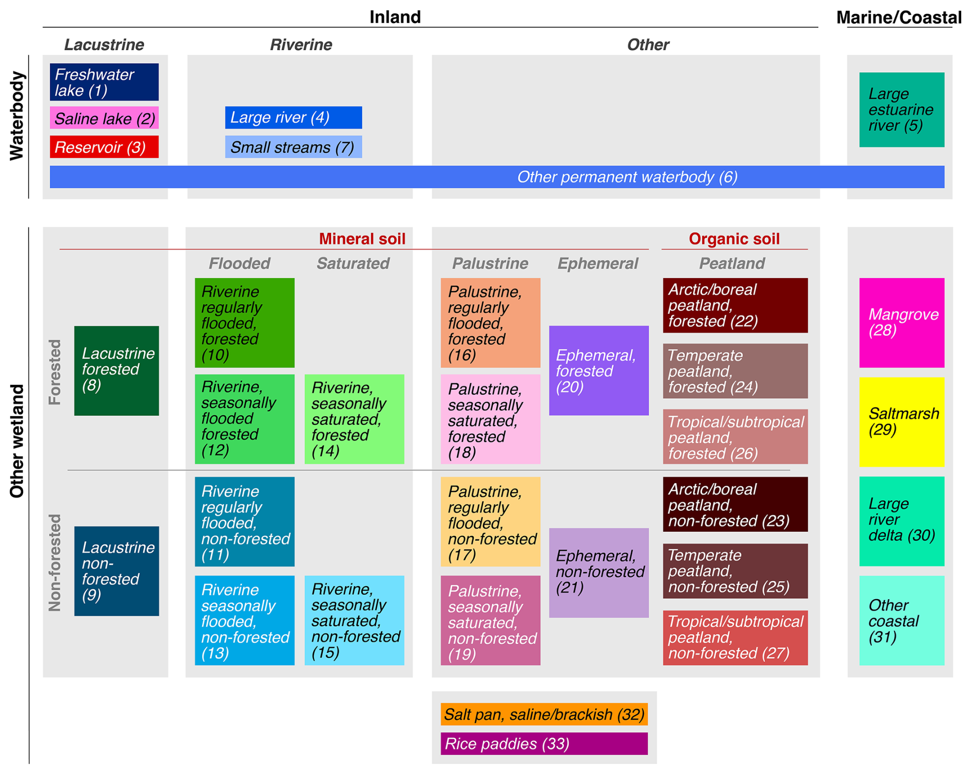
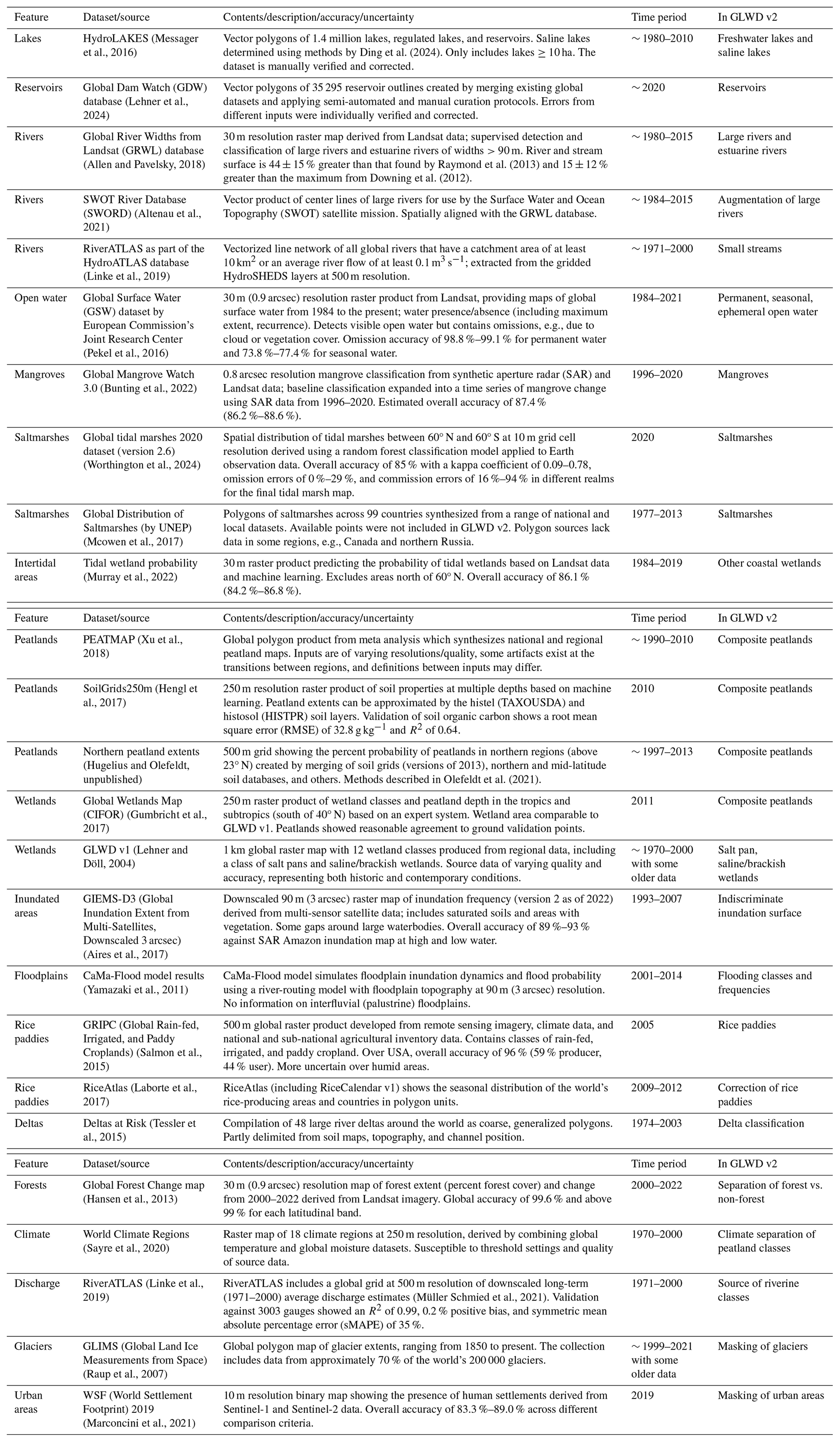
Figure 2 Schematic of classification hierarchy and distinctions among the 33 classes represented in GLWD v2. At the highest level, classes are grouped into four realms resulting from the 2 × 2 combinations of the overarching wetland division (waterbody vs. other wetland, including emergent and bare wetlands) with landscape position (inland vs. marine/coastal). Inland waterbodies and other wetlands are then further divided according to water source and dynamic – lacustrine (lentic), riverine (lotic), and other (including palustrine and peatland). Other characteristics, such as soil type (mineral vs. organic) and vegetation cover (forested vs. non-forested) can be used to regroup wetland classes across water sources. Finally, mineral wetlands are further separated by their hydrological conditions (flooded vs. saturated) and regimes (ephemeral).

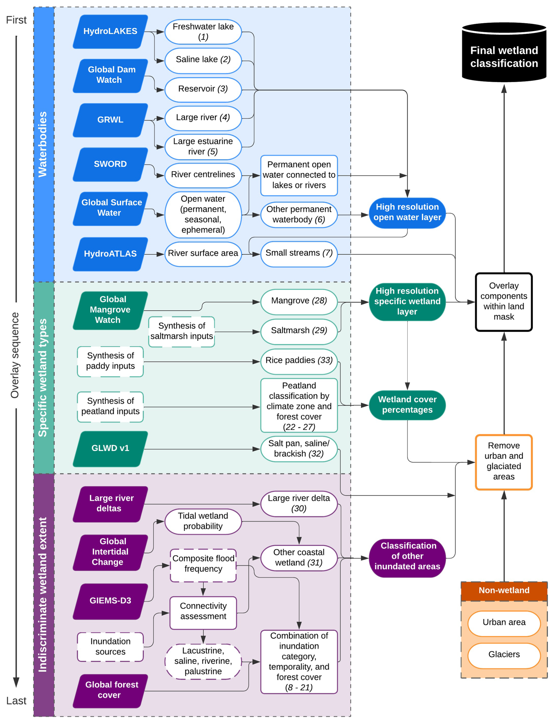
Figure 3 Schematic of the workflow and main processing steps to create GLWD v2. The processing steps are grouped into three main parts, corresponding to Sect. 3.2 (top, blue), 3.3 (middle, green), and 3.4 (bottom, purple) of the text. Input datasets are represented by parallelograms, while processes are represented by boxes. Interim and final layers and classes are represented by ovals, with class numbers indicated in parentheses after each class name. Input datasets and results of each section are shown in solid shading. Shapes with dashed outlines represent complex processes with inputs that are not specifically described in this diagram; the details of these steps and their source data are explained in the text. This schematic broadly indicates the sequential order in which the different datasets were combined (from top to bottom equals first to last); however, some wetland types were reclassified or grouped together to produce the final set of 33 classes, as described in Sect. 3.2–3.4. A more detailed version of this schematic with additional sub-steps is provided in Fig. B1 (Appendix B).

3 Methods

3.1 Overview of methodology

The guiding principle for creating GLWD v2 was to consolidate and harmonize – without duplication – all input data sources to produce a versatile global map of wetland types that is useable in a broad spectrum of applications. Antarctica was excluded from the mapping efforts due to generally incomplete or unreliable spatial input data. Results are provided as a series of grids with a target cell size of 15 arcsec (∼ 500 m), which was chosen as a compromise between the spatial resolution of existing input data sources, computing demands, and ease of use for global applications. It is important to note, however, that the information from finer-resolution input data, including permanent water surfaces at ∼ 30 m and saltmarshes at ∼ 10 m resolution, is preserved in the fractional cell coverage of each wetland type. The classification scheme of GLWD v2 (Fig. 2) is designed to be manageable (i.e., limited to a reasonable number of classes), expert-guided rather than statistically derived, and representative of the needs of various research fields and disciplines. Each of the 33 wetland classes is provided as an individual global map depicting the extent of the respective class as cell fractions. The 33 maps are then combined to derive the total global wetland extent and to identify the dominant wetland class per grid cell.

The main processing steps of GLWD v2 are outlined in Fig. 3 and are described in more detail in Sect. 3.2 to 3.5. The central procedure combines four types of data: (a) high-resolution data of waterbodies, (b) data of various resolutions of other wetland types, (c) high-resolution downscaled or modeled data of indiscriminate inundated areas, and (d) ancillary data to support the classification of indiscriminate wetland types and the refinement of classes.

For the merger, higher-quality data sources were assigned priority over lower-quality ones based on reliability, precision, resolution, confidence, completeness (in time and space), coherence, and information content (e.g., classified vs. unclassified data). When these criteria were ambiguous or conflicting (e.g., higher resolution but lower confidence), the prioritization of input datasets was guided by expert decision. The sequential merger of data layers was performed by a process we hereafter refer to as “inserting” wetland extents, whereby the next lower-priority layer is successively allowed to occupy the grid cell space that remains free after all higher-priority waterbodies and wetlands have been processed (analogous to “mosaicking” in GIS terminology). Data sources representing waterbodies were first combined following the order: lakes > reservoirs > rivers > other subclasses. Next, data sources depicting individual wetland types were inserted around the waterbodies, followed by indiscriminate inundated areas that were subsequently classified using ancillary information. Thus, predominantly permanent waterbodies were spatially allocated first, and mostly non-permanent wetland extents were inserted thereafter to complement and surround these waterbodies. Finally, the map was refined by masking urban (built-up) and glaciated areas.

The sequential merger of multiple layers of different original resolutions to one common layer results in a combined grid where multiple wetland types can overlap in a 15 arcsec output cell. Importantly, the sequence of layer stacking ensures that higher-level (finer) features are systematically subtracted from lower-level (coarser) ones during the overlay and insertion process. This eliminates – or at least reduces (depending on spatial precision and resolution of data sources) – double counting in cases of spatial overlap and asserts that the summed waterbody and wetland coverage is bounded by the total area of each output cell.

3.2 Processing of waterbodies

Figure 3 illustrates the main processing steps of this section in blue color (top panel), and all data sources are listed in Table 1. The input datasets of waterbodies were processed globally at 1 arcsec (∼ 30 m) resolution, except for small streams, which were processed at 15 arcsec (∼ 500 m) resolution. Some preprocessing steps were executed at higher resolutions (see details below).

3.2.1 Lakes, saline lakes, and reservoirs (classes 1–3)

Lakes were extracted from the polygons of the HydroLAKES database (Messager et al., 2016), which contains ∼ 1.4 million lakes globally with a size of at least 10 ha. We converted the lakes of HydroLAKES v1.1 (including regulated lakes but excluding reservoirs) to a raster layer at 1 arcsec resolution according to whether at least half of each grid cell area was covered by a lake polygon. Reservoirs were extracted from the Global Dam Watch (GDW) database v1.0 (Lehner et al., 2024), which contains 35 295 reservoir polygons globally, applying the same polygon to raster conversion as for lakes. It should be noted that HydroLAKES and the GDW database are spatially complementary and thus do not include any overlapping polygons.

Furthermore, we distinguished saline lakes (assuming a relatively high salinity threshold of 30 ppt, i.e., 30 g L⁻¹) using a classification framework based on hydrography datasets, satellite imagery, and literature documentation as described in Ding et al. (2024). The supervised classification identified a total of 24 374 saline lakes, mostly located in endorheic (closed) inland depressions and arid or semi-arid climate zones. These conditions are conducive to salinity accumulation due to a lack of surface outflow, strong potential evaporation, or both. Many of the detected saline lakes exhibit lacustrine evaporites visible from satellite images. To evaluate the overall robustness of the classification method, we conducted an independent literature search for all lakes exceeding 500 km² in surface area which confirmed that all 66 reported saline lakes (with salinity levels exceeding 3 g L⁻¹) in that size class were correctly detected in the supervised classification and only 1 saline lake from the supervised classification required conversion to non-saline.

3.2.2 Rivers and estuarine rivers (classes 4–5)

Rivers and estuarine rivers were extracted from the raster layers of the Global River Widths from Landsat (GRWL) database (Allen and Pavelsky, 2018). It should be noted that the original GRWL data also offer a lake class, but we used this class only as a component layer to identify and conserve critical connections between lakes and their in- or outflowing river courses. After Sect. 3.2.3 below, the lake class from GRWL was discarded to avoid double counting lakes.

We reprojected and resampled all published 10 × 10° GRWL tiles from their original 30 m resolution and Universal Transverse Mercator (UTM) projection to match the geographic coordinate system of GLWD v2 at a 0.25 arcsec (∼ 8 m) resolution. The resulting high-resolution tiles were then aggregated and merged to create a seamless global layer that retained all 1 arcsec cells with at least 50 % river coverage. The GRWL tiles can exhibit minor gaps at their edges when combined into a seamless global coverage, which we rectified by inserting data inside a 0.1° buffer around all edges from an unpublished version of GRWL (provided by the authors) of slightly inferior quality but with overlapping tiles.

To further ensure connectivity between river surfaces and adjacent lakes in the subsequent combination steps, we also processed and inserted the related vector product of the Surface Water and Ocean Topography (SWOT) River Database (SWORD) (Altenau et al., 2021), which presents center lines for all GRWL rivers, including their paths traversing through lakes. We converted these vector lines to a grid at 1 arcsec resolution, added a one-cell buffer to produce slightly wider river lines, and retained only those SWORD cells that coincided with a GRWL lake. Furthermore, as the SWORD river center lines can cross land, such as over islands within a braided river system, we removed all SWORD river cells farther than one cell from the permanent open water class of the Global Surface Water (GSW) dataset (see next step).

3.2.3 Other permanent waterbodies (class 6)

We used the Global Surface Water (GSW) dataset (Pekel et al., 2016) to complement the lakes, reservoirs, and rivers. GSW offers gridded data at 0.9 arcsec resolution (∼ 27 m) compiled from Landsat imagery spanning the years 1984 to present. We used the separation of GSW into permanent, seasonal, and ephemeral classes from its transitions layer for the years 1984 to 2020 and resampled it to our target 1 arcsec resolution. Cells labeled as seasonal or ephemeral and coinciding with a GRWL lake were reclassified as permanent to conserve the lake–river connections in subsequent steps. We then inserted permanent GSW cells as their own waterbody class in GLWD v2, which nominally includes – but does not distinguish between – small lakes, ponds, rivers, and canals that exceed the 27 m detection threshold of GSW and have not been depicted in any of the other waterbody datasets. Furthermore, due to spatial inaccuracies and misalignments of the GLWD v2 land mask along the marine coastline, this class also includes some near-shore marine waters and tidal flats that have been depicted in GSW as permanent water. The seasonal and ephemeral classes were integrated into the classification of other wetlands in subsequent steps (Sect. 3.4).

3.2.4 Combination of waterbody classes and reclassification of some cells

We combined the open waterbody features at the 1 arcsec resolution described in the previous steps by overlaying them in the following priority order: freshwater lake > saline lake > reservoir > river > estuarine river > other permanent waterbody. In instances where waterbody boundaries were misaligned in the source datasets (e.g., a lake from HydroLAKES may not cover the entire permanent water from GSW or a gap exists between the outlines of hydrologically connected lakes and rivers), we reclassified some of the gap cells of GSW from other permanent waterbody to the type of the adjacent waterbody. This reclassification was performed based on proximity along contiguous cells from the waterbodies up to a maximum distance of 0.002° (∼ 200 m).

3.2.5 Adding small streams (class 7)

The surface extent of small rivers and streams is not well captured in global remote sensing imagery due to the narrow, linear features in sub-meter dimensions (Allen et al., 2018). To account for this omission, a statistical estimate of the surface area of small streams was produced using river area estimates from the RiverATLAS database (Linke et al., 2019), which in turn were derived from downscaled discharge estimates (Müller Schmied et al., 2021) and simple hydraulic geometry laws (Allen et al., 1994). The total surface area of rivers and streams was calculated by multiplying the estimated channel width and length of every river reach that exceeds 10 km² in catchment area or 0.1 m³ s⁻¹ (100 L s⁻¹) in average flow in each 15 arcsec grid cell (Linke et al., 2019). To represent only small streams and avoid double counting, with larger rivers already mapped by GRWL (Sect. 3.2.2), the GRWL river extent was subtracted from the total river area provided by RiverATLAS in each 15 arcsec cell. Given the uncertainty of this estimation method, small streams were given the lowest priority among all waterbodies. Finally, the maximum extent of small streams was limited to 10 % of each 15 arcsec cell (∼ 2.5 ha), which resembles a river reach of approximately 500 m length (one cell) and 50 m width, as the GRWL and GSW products should cover rivers exceeding this size even if not coinciding within a given cell due to potential spatial mismatches. It should be noted that while small streams are grouped within the waterbody classes of GLWD v2, 50 %–60 % of small streams globally have been estimated to be intermittent or ephemeral (Messager et al., 2021).

3.3 Processing of explicit wetland types

Figure 3 illustrates the main processing steps of this section in green color (middle panel), and all data sources are listed in Table 1. Datasets representing the distribution of explicit wetland types were processed globally at 0.3, 1, 3, or 15 arcsec resolution (∼ 10, 30, 90, or 500 m, respectively) depending on their native data format.

3.3.1 Insertion of high-resolution coastal wetlands (classes 28–29)

We used original high-resolution source data to define the extent of three explicit coastal wetland types at the target processing resolution of 1 arcsec (∼ 30 m): mangroves (Bunting et al., 2022), saltmarshes (Worthington et al., 2024; Mcowen et al., 2017), and intertidal areas (Murray et al., 2022). The mangrove class was produced from the maximum mangrove extent in the source data after resampling from its original 0.8 arcsec resolution. The saltmarsh class was created by first resampling the original ∼ 10 m resolution tiles of the dataset by Worthington et al. (2024) and converting all provided saltmarsh polygons of the dataset by Mcowen et al. (2017) to the target 1 arcsec resolution. Given the lower accuracy and completeness of the dataset by Mcowen et al. (2017), it was only used for regions north of 60° N, where no data from Worthington et al. (2024) existed. The intertidal wetland areas, which were later integrated into the other coastal wetland class (see Sect. 3.4.3), were resampled from their original ∼ 30 m resolution, and all grid cells with a given probability of inundation of at least 50 % were retained. The three classes were then inserted into the map of harmonized waterbody classes (result of Sect. 3.2), giving priority to waterbodies followed by mangroves > saltmarshes > intertidal areas.

3.3.2 Masking of urban and glaciated areas

Up until this step, all previous data sources were included into GLWD v2 without further corrections because they met sufficiently high standards of spatial accuracy and detail. Before adding coarser-resolution information, however, high-resolution non-wetland masks for urban areas and glaciated areas were inserted at the 1 arcsec resolution to prevent subsequent steps from allocating wetlands to these surfaces. The urban areas were aggregated from the original 10 m resolution of the World Settlement Footprint 2019 binary mask (Marconcini et al., 2021) to produce a percentage cover at 1 arcsec resolution, and cells with at least 50 % settlement cover were classified as urban. Glaciated areas (Raup et al., 2007) were converted from their original polygon format to the target 1 arcsec resolution. At the end of all processing steps, i.e., before the creation of the final GLWD v2 maps (Sect. 3.5), the urban and glaciated classes were discarded and replaced by the dryland (non-wetland) class.

3.3.3 Insertion of rice paddies (class 33)

Rice paddy extents (Salmon et al., 2015) were inserted as percent coverage into all remaining unoccupied areas. The original grid – which delineates global rice paddy extents at 500 m resolution based on a predictive model – included numerous artifacts, such as erroneous small patches over regions with no known rice production. Furthermore, under realistic conditions, rice paddies typically form only part of a heterogeneous landscape mosaic, where rice fields intersperse with other agriculture, roads, and small settlements, i.e., where, at a 500 m resolution, each grid cell is covered by less than 100 % rice paddies. We therefore converted the rice paddy layer from its original binary format to a fractional 0 %–100 % range using several preprocessing steps. After reprojecting and resampling the original data to the target geographic coordinate system and 15 arcsec cell resolution of GLWD v2, we calculated each 15 arcsec cell's rice fraction as the percentage of the original rice paddy extent found within a distance of ∼ 2 km around the cell (i.e., in a 9 × 9 cell neighborhood). We then used the administrative areas available as part of the RiceAtlas (Rice Calendar v1; Laborte et al., 2017) to discard regions where no paddy rice production is reported (after some minor manual corrections). Finally, the maximum rice paddy extent within a grid cell was capped at 50 % and any rice paddy coverage below 20 % was considered an inherent data error (mostly occurring along marine coastlines) and was removed. These thresholds, besides delivering visually plausible rice paddy regions, were chosen in an iterative trial-and-error process to approximately match the reported global rice paddy extent of ∼ 1.2 ×10⁶ km², as well as the reported extents of the two dominant rice producing countries of India (∼ 400 000 km²) and China (∼ 250 000 km²) (see Table 4 in Results for sources).

3.3.4 Insertion of peatlands (classes 22–27)

Several global or near-global peatland extent maps have been developed in the past, each with its own specificities, strengths, and weaknesses, which led us to conclude that no single data product is of sufficient quality and/or completeness to represent all peatlands in GLWD v2. Therefore, we created a new composite peatland probability map from four input datasets (Table 1): PEATMAP (Xu et al., 2018; global), SoilGrids250m (Hengl et al., 2017; global), Northern Peatlands (Hugelius and Olefeldt, unpublished; north of 23° N), and CIFOR (Gumbricht et al., 2017; south of 40° N, of which we only used data south of 23.5° N). The four input datasets were first reprojected and/or resampled into the geographic coordinate system of GLWD v2 and converted to a peatland percentage cover in each 15 arcsec grid cell as follows.

PEATMAP originally offers spatial peatland percentages for regions in Canada and some areas in eastern Asia (0 %–100 %) and otherwise binary presence/absence information, which we set to 100 % and 0 %, respectively. PEATMAP is provided in polygon format which we corrected for some slight locational misalignments across Oceania and some regions of eastern Asia. Also, individual polygon parts with an area <20 ha (i.e., smaller than one grid cell in our target 15 arcsec resolution) were removed as upon visual inspection, many of them represented spurious outliers and artifacts rather than precise peatland boundaries. SoilGrids250m offers cumulative probabilities (0 %–100 %) of Histosols occurring in any 250 m grid cell globally as well as an independent probability of Histels. We used the maximum value of Histosols or Histels per 15 arcsec cell and interpreted the result as the spatial probability of peatland occurrence in percentages. The Northern Peatlands grid is based on the same underpinning data and methods as presented in Olefeldt et al. (2021) and was reproduced here as a 15 arcsec grid specifically for the purpose of inclusion in GLWD v2. It offers the percent peatland extent per grid cell for Histosols and Histels, separately, which we summed into one grid (0 %–100 %). Finally, the CIFOR dataset includes a binary peatland classification, which we interpreted as 0 % or 100 % coverage, respectively. Furthermore, to avoid abrupt spatial transitions in the binary information of CIFOR, we inserted the values from SoilGrids250m wherever CIFOR showed zero values.

After standardization, the four layers of peatland probabilities were combined into an equally weighted average; i.e., by calculating the average of the respective three input grids that existed north of 23.5° N and south of 23° N, and the average of all four input grids in the 0.5° transition zone using an edge smoothing (blending) approach. Calculating averages ensures that final extent probabilities remain within 0 % and 100 % and that the total global peatland extent falls within the individual estimates of the input datasets. We removed values below 3 % from the final composite peatland map as these low percentages occurred throughout the globe including in areas of no known peatland extent, mostly due to artifacts of low probabilities inherent in the SoilGrids250m product of Histosols and Histels.

To create three climatological peatland types, we combined the composite peatland map with reclassified climate zones from the World Climate Regions (Sayre et al., 2020), which we first resampled from the original ∼ 250 m to 15 arcsec resolution. We separated peatlands into arctic/boreal (original polar and boreal climates), temperate (original cool and warm temperate climates), and tropical/subtropical (original tropical and subtropical climates), and we applied a manual adjustment in that arctic/boreal climates were reclassified to temperate in regions below 43° N (with some additional adjustments of small non-contiguous areas between 43 and 55° N) to avoid the occurrence of minor arctic/boreal peatlands within tropical/subtropical mountains.

Finally, each of the three peatland classes was further subdivided into forested and non-forested using the same ancillary forest data and approach as described in more detail in Sect. 3.4.3 below. The six resulting combinations of climatological and forested/non-forested peatland classes were then inserted into GLWD v2.

3.3.5 Insertion of salt pans, saline and brackish wetlands (class 32)

In the absence of better global information, the extent of salt pans and saline/brackish wetlands was taken from the gridded version of GLWD v1 and disaggregated from its original 30 to 15 arcsec resolution. The salt pans and saline/brackish wetlands were assumed to occupy 100 % of the original grid cells. Before insertion into GLWD v2, this class was augmented with the saline class derived in Sect. 3.4.2 below. An exception to our fusion rules was made in that this class could later be replaced by the two wetland types, large river delta and other coastal wetland (see Sect. 3.4.3), as these two classes were considered more reliable than the coarse GLWD v1 product.

3.4 Processing and classification of indiscriminate wetland extents

Figure 3 illustrates the main processing steps of this section in purple color (bottom panel), and all data sources are listed in Table 1. Datasets representing the distribution of indiscriminate wetland extents were processed globally at 3 arcsec (∼ 90 m) resolution. First, an all-encompassing global inundation extent map was created, which was then classified using ancillary data and an analysis of connectivity to the nearest waterbody.

3.4.1 Determination of maximum inundation extent and flood frequencies

We created an indiscriminate maximum inundation extent map at 3 arcsec resolution and assigned flood frequency values to each cell by combining four input datasets: (a) the downscaled GIEMS-D3 inundation data at 3 arcsec resolution over 1993–2007 (Aires et al., 2017), which formed the majority of the maximum extent as it includes both permanent open water and temporary wetlands; (b) the waterbody layer of GLWD v2 produced in Sect. 3.2.1 to 3.2.4 at 1 arcsec resolution (i.e., without small streams); (c) the seasonal and ephemeral open water cells of the GSW datasets at 1 arcsec resolution; and (d) the flooded extent simulated by the CaMa-Flood model as inundated for more than 7 d per year at 3 arcsec resolution (Yamazaki et al., 2011). The 1 arcsec input datasets were aggregated to 3 arcsec resolution by defining each 3 arcsec grid cell as inundated if it contained at least one wetland cell at 1 arcsec resolution.

All four inundation data sources were combined by extracting the maximum inundation frequency (0 %–100 %) per grid cell among the sources. With its broad coverage, the GIEMS-D3 database provided most of the inundation frequency estimates (0 %–100 %) but was supplanted by the following (wherever they occurred and showed higher inundation frequencies): GLWD v2 waterbodies (assumed to have 100 % inundation frequency as most of these waterbodies are permanent), seasonal GSW cells (80 % inundation frequency, broadly based on GSW statistics), CaMa-Flood inundation (10 % inundation frequency, slightly above the applied minimum inundation threshold of 7 d per year), or ephemeral GSW (5 % inundation frequency, GSW statistics).

3.4.2 Division of indiscriminate inundation into broad categories using hydrological connectivity

In order to classify the wetlands encompassed by the indiscriminate inundation extent, we first stratified the maximum extent map (Sect. 3.4.1) into one of five broad water source categories: lacustrine, saline, riverine, coastal, and palustrine – which we then further refine in Sect. 3.4.3 below. These five categories were derived by determining the nearest hydrologically connected flooding source (waterbody, ocean, or local runoff) for each indiscriminate inundation cell, with hydrologic connectivity and distances being measured along flow paths between contiguous wetland cells. The flooding sources for the five categories originated from the previously assigned GLWD v2 classes, such that cells nearest to freshwater lakes or reservoirs were classified as lacustrine, cells nearest to saline lakes as saline, cells nearest to rivers as riverine, cells nearest to estuarine rivers or the ocean as coastal, and all other cells disconnected from a source as palustrine.

Several additional criteria were applied in the determination of connectivity and proximity, and all parameters and thresholds were set by expert judgment guided by visual comparisons to known wetland complexes. We used the flood frequency map (Sect. 3.4.1) as input to trace paths of flooding between every inundated cell and its most likely source of flooding. The most plausible connectivity was determined through a custom algorithm which ensured that the shortest flow paths followed preferential flow directions from each cell towards the neighboring cell with highest flood frequency while remaining within contiguous inundation cells. This approach permits cells to be assigned a more spatially distant source if the flood frequencies are higher along that path. The process development and thresholds of lacustrine and coastal source attribution (see below) were informed by visual comparisons with the elevation range from variations in lake surface water elevations observed by ICESat-2 (Cooley et al., 2021) and along coastlines by a reanalysis of tides and surges (Muis et al., 2022).

Two iterations of the connectivity assessment were performed. First, connectivity along cells with flood frequencies ≥80 % was determined to represent more persistent inundation and direct connectivity of wetlands fringing their adjacent waterbodies. This iteration was assumed to fully define the lacustrine and saline categories and they were removed from the following iteration. Second, unassigned inundated cells were categorized into riverine and coastal with an expanded connectivity assessment over cells of >10 % inundation frequency and using previously assigned riverine and coastal cells as additional sources. Also, riverine sources were supplemented in the second iteration by cells with a long-term average discharge exceeding 1 m³ s⁻¹ from the RiverATLAS database (Linke et al., 2019). During both iterations, grid cells with an elevation above 10 m a.s.l. were excluded from becoming coastal. All grid cells without an assigned category after both iterations, signifying no surface hydrological connectivity to flooding sources, were labeled as palustrine.

Table 2 Thresholds used to define lacustrine, riverine, palustrine, and ephemeral wetland classes.

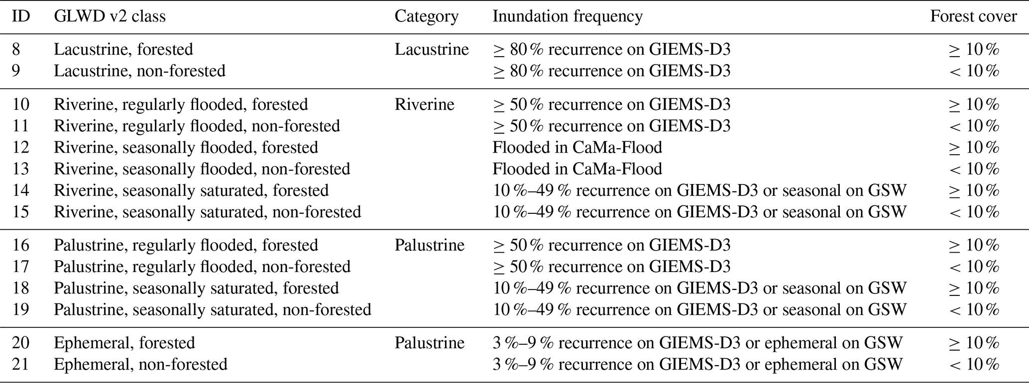
3.4.3 Final classification of indiscriminate wetlands with ancillary data (classes 8–21, 30, and 31)

The lacustrine, riverine, and palustrine categories were further subdivided into 14 classes based on inundation frequencies and forest cover (Table 2). Due to the thresholds used in the previous step, the only category containing grid cells with inundation frequencies below 10 % was palustrine. These palustrine wetlands with low-frequency flooding were further constrained to a minimum frequency of 3 % to remove the highly uncertain representation of rarely inundated extents in GIEMS-D3 data and then relabeled as ephemeral.

Forest cover (Hansen et al., 2013) was used to separate between wetlands that fit the general definition of forested swamps vs. non-forested freshwater marshes. For this process, the percent tree cover values were first resampled by averaging from the original 0.9 to 3 arcsec resolution. To also accommodate shrubbed swamps, we set a relatively low threshold of 10 % tree coverage for forested wetlands, which was visually calibrated to match known swamp occurrences, including parts of the Pantanal in South America; the Tonle Sap freshwater swamp forests in Asia; and the Sudd, Okavango, Bangweulu, and Niger Delta swamps in Africa.

Large river deltas were discerned as an additional class within the indiscriminate inundation areas using ancillary information. We converted the polygons of large river deltas (Tessler et al., 2015) to a grid at 3 arcsec resolution, and because of their low-precision outlines, we extended them with a ∼ 1 km buffer (15 grid cells) to avoid spurious gaps at the land–ocean boundary. Delta areas were clipped to the extent of the maximum inundation map (Sect. 3.4.1). The large river delta class (no. 30) superseded all other classes of the indiscriminate inundation areas.

Furthermore, we grouped a small number of conceptually similar classes to simplify and eliminate ambiguities: outside of large river deltas, the coastal wetland category was combined with the intertidal wetlands (Sect. 3.3.1) to form the other coastal wetlands class (no. 31); and the saline wetland category was added to the salt pan, saline/brackish wetland class (Sect. 3.3.5).

Finally, all lacustrine, riverine, palustrine, ephemeral, coastal, and saline classes derived for the indiscriminate wetland areas were inserted into the remaining open grid cell spaces of GLWD v2.

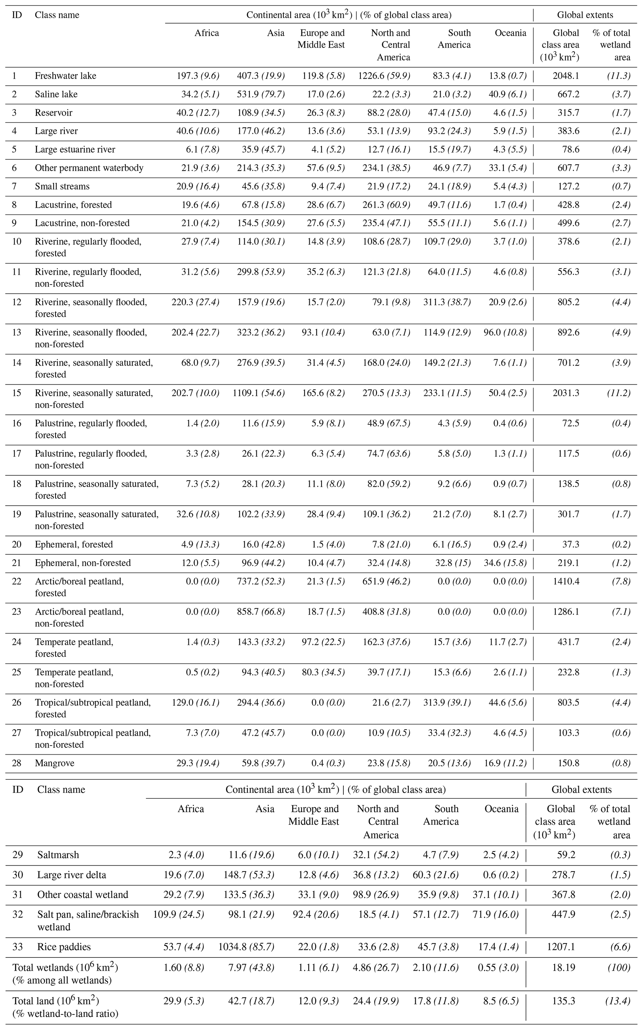
Table 3 Continental and global extents of GLWD v2 wetland classes. Values in parentheses represent the continent's percent of the global extent of each class, except for the two bottom rows which refer to all wetlands globally. Areas are in 10³ km², except for totals in the two bottom rows, which are in 10⁶ km². Asia includes all of Russia; North America includes Greenland; Oceania includes Australia, New Zealand, Melanesia, Micronesia, and Polynesia; and total land area excludes Antarctica. A breakdown of all wetland classes by country is available in the Supplement. The values in italics refer to percentages.

3.5 Creation of final GLWD v2 maps

For each of the 33 GLWD v2 wetland classes, an individual global grid was produced at the output 15 arcsec resolution, showing the percent coverage of the respective wetland class per grid cell. In addition, the resulting spatial extents of all wetland classes were summed for each cell, creating a total global wetland extent map (the maximum total extent was capped at 100 % where rounding caused slight exceedances). These 34 fractional maps were also produced to show absolute areas (in ha) per grid cell – using geodesic calculations – for ease of application. Finally, the dominant wetland class per grid cell (i.e., the class showing the highest fractional wetland coverage per cell) was determined to create a single global map of wetland types. In cases of ties, the dominant class was assigned to be the lower class number.

4 Results

GLWD v2 distinguishes 7 waterbody types and 26 other wetland types for a total of 33 distinct non-overlapping classes (Table 3). It provides a static snapshot of the inland surface water extent and climatology for contemporary conditions centered around the period 1984–2020, which represents the varying time periods of most of its input data (see Table 1). Its nominal spatial resolution is 15 arcsec (∼ 500 m), yet it provides cell fractions of wetland cover that are derived from water surfaces at resolutions as fine as 0.3 arcsec (∼ 10 m) to preserve smaller waterbodies. This database surpasses its predecessor, GLWD v1 (Lehner and Döll, 2004), in detail, consistency, and comprehensiveness to serve a broad range of applications by offering a composite global map of wetland ecosystem types.

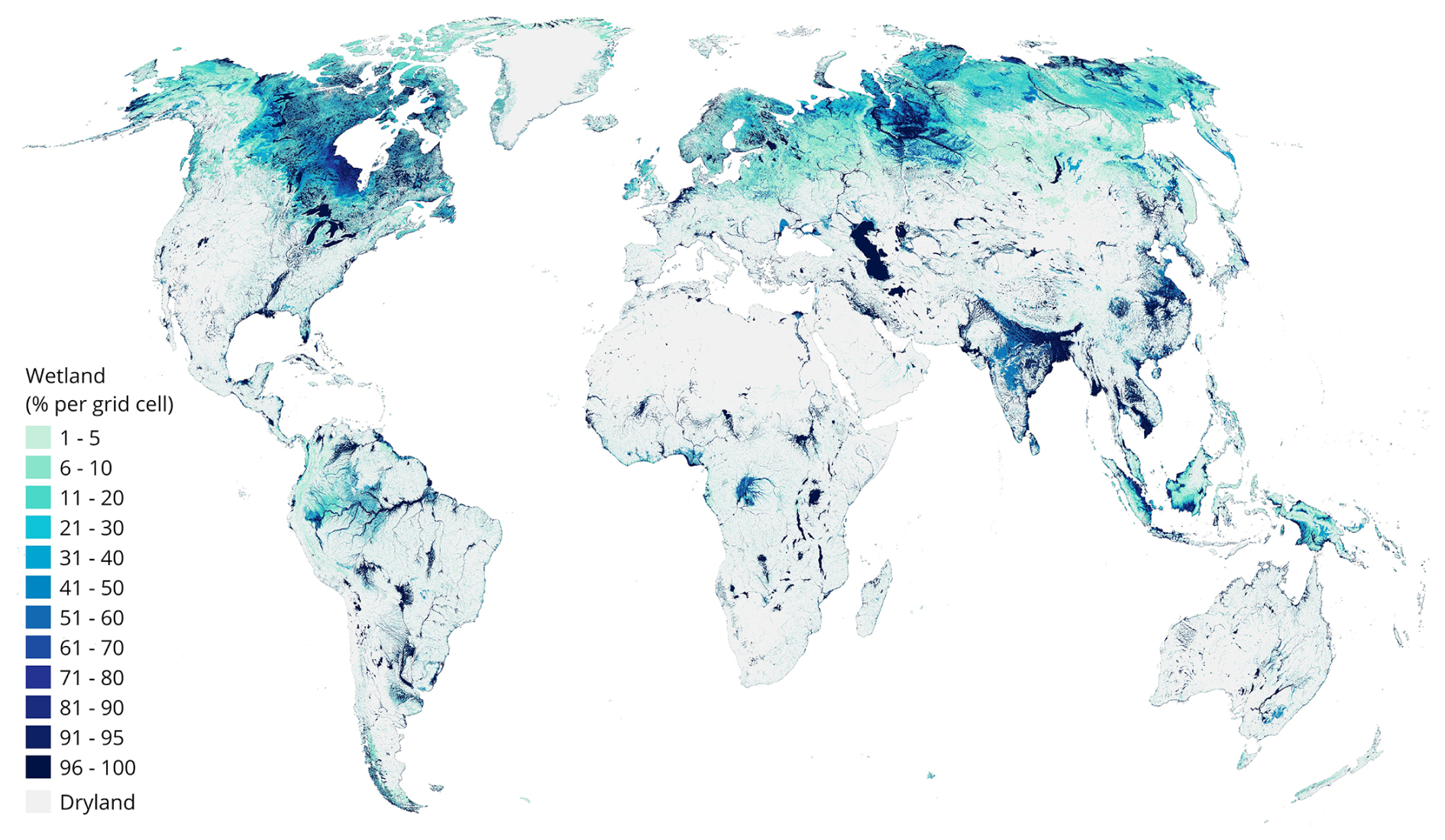
Figure 4 Total wetland extent as estimated by the Global Lakes and Wetlands Database (GLWD) v2. Values show the combined fractional coverage of all wetland classes per 500 m grid cell. Total wetland extent in each cell is bounded to 1 %–100 %; cells with 0 % wetland extent are classified as dryland.

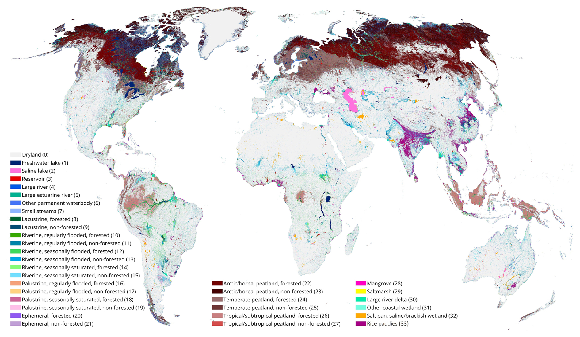
Figure 5 Dominant wetland class for each 500 m grid cell of the Global Lakes and Wetlands Database (GLWD) v2. Total wetland extent in each cell is bounded to 1 %–100 %; cells with 0 % wetland extent are classified as dryland. Legend classes include numerical class values in parentheses.

4.1 Global wetland extent

The total combined extent of all wetland classes in GLWD v2 including all inland and coastal waterbodies and wetlands of all inundation frequencies – that is, the maximum extent – covers 18.2 ×10⁶ km², equivalent to 13.4 % of the total global land area excluding Antarctica (Table 3). Most wetlands are found in Asia (43.8 % of global wetland extent) followed by North and Central America (26.7 %). These two continents also show the highest wetland-to-land ratios (18.7 % and 19.9 %, respectively), while Africa and Oceania exhibit the lowest wetland ratios (5.3 % and 6.5 %, respectively). Regions with high densities of wetlands include southern and southeastern Asia, in part due to large swaths of paddy rice fields; the tropics, where large riverine complexes exist; and areas north of ∼ 45° N, where lakes and peatlands dominate the landscape (Figs. 4 and 5). Overall, the patterns of global wetland distribution correspond closely with regional climatic, physiographic, and hydrologic conditions and generally agree with the results from the compilation of multiple wetland inventories undertaken by Davidson et al. (2018).

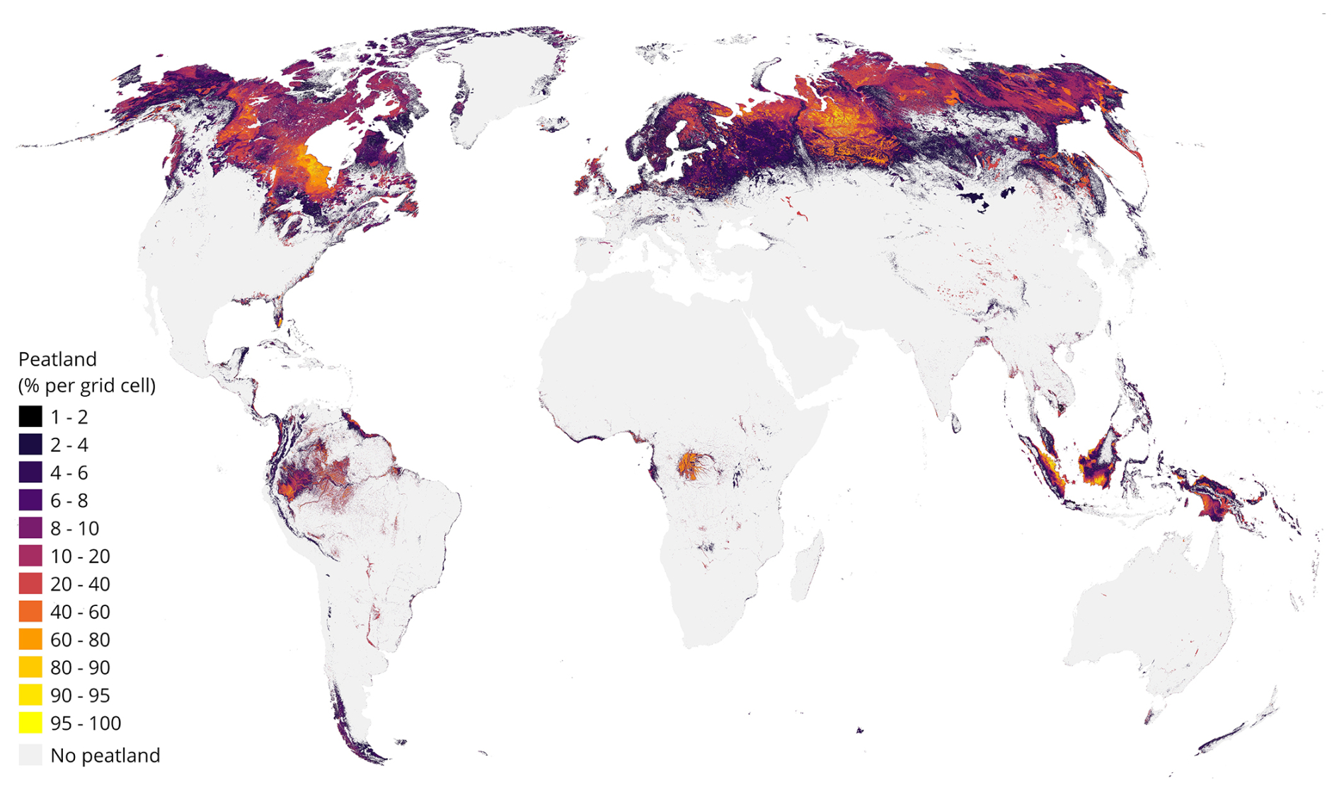
Figure 6 Total peatland extent as estimated by the Global Lakes and Wetlands Database (GLWD) v2 for all six peatland classes combined (arctic/boreal, temperate, and tropical/subtropical; forested and non-forested). Values show fractional coverage per 500 m grid cell. Total peatland extent in each cell is bounded to 1 %–100 %; cells with 0 % peatland extent are classified as no peatland.

4.2 Wetland class distribution

Grouping specific classes into broad categories reveals global trends of wetland distribution. Unsurprisingly, marine/coastal wetland classes cover only 5 % of the total extent, while the majority of 95 % of wetlands are inland. Waterbody classes occupy 23 % of the total wetland extent, while other wetland classes, including emergent and bare wetlands, occupy 77 %. Freshwater marshes (i.e., non-forested) and freshwater swamps (i.e., forested) (combined classes 8–21) compose 39 % of all wetlands, with two-thirds being marshes (64 %) and one-third swamps (36 %). Within these marsh and swamp areas, the vast majority (68 %) is seasonally flooded or saturated, highlighting the strong intra-annual variability of these wetlands, while 16 % are regularly flooded, 4 % are ephemeral, and 13 % are lacustrine wetlands with no specified periodicity (total not summing to 100 % due to rounding). When these marsh and swamp wetlands are grouped by flooding source, riverine wetlands account for the largest share (75 %), followed by lacustrine (13 %), palustrine (9 %), and ephemeral (4 %) wetlands.

A more granular inspection of individual classes highlights the predominance of specific wetland types. Among the 33 classes (Table 3 and Fig. 5), 5 classes exceed 1 ×10⁶ km² globally: freshwater lakes (2.05 ×10⁶ km², of which 60 % are in North and Central America); riverine, seasonally saturated, non-forested wetlands (2.03 ×10⁶ km²); forested arctic/boreal peatlands (1.41 ×10⁶ km²); non-forested arctic/boreal peatlands (1.29 ×10⁶ km²); and rice paddies (1.21 ×10⁶ km²). All peatlands combined (arctic/boreal, temperate, and tropical/subtropical, both forested and non-forested) cover a total of 4.27 ×10⁶ km², representing nearly a quarter (23 %) of the total wetland extent on Earth (Table 3 and Fig. 6). They emerge as the dominant wetland type across almost all northern latitudes above 50° N as well as parts of the tropics; however, as the organic soils of peatlands are difficult to map with remote sensing methods, the coarser resolution of the input source data used in GLWD v2 creates local uncertainties. Rice paddies (6.6 % of total global wetland extent) occur predominantly throughout southern and eastern Asia, including India, northeast China, Vietnam, Thailand, Bangladesh, Sri Lanka, and Myanmar, and, to a lesser extent, other regions such as the Nigerian coast and within the Mississippi floodplains (Fig. 5). Various other waterbody and wetland classes are regionally dominant, including freshwater lakes in North America and northern Eurasia; riverine wetlands in South America, sub-Saharan Africa, and Asia; saline lakes in central Asia; and ephemeral wetlands in Australia. Small streams occur at small percentages all around the world and dominate in locations where no other wetland type occurs; but they are not easily discernable on the global map (Fig. 5) among other more prominent wetland classes. A breakdown of all wetland classes by country is available in the Supplement.

Table 4 Comparisons of global and regional wetland extents. Data sources used in the comparison include field-based surveys, remote sensing products, expert assessments, meta analyses, and national statistics. Regional estimates are shown in italics. More details on the main characteristics and methodological approach of each referenced literature source are provided in Table A2 (Appendix A).

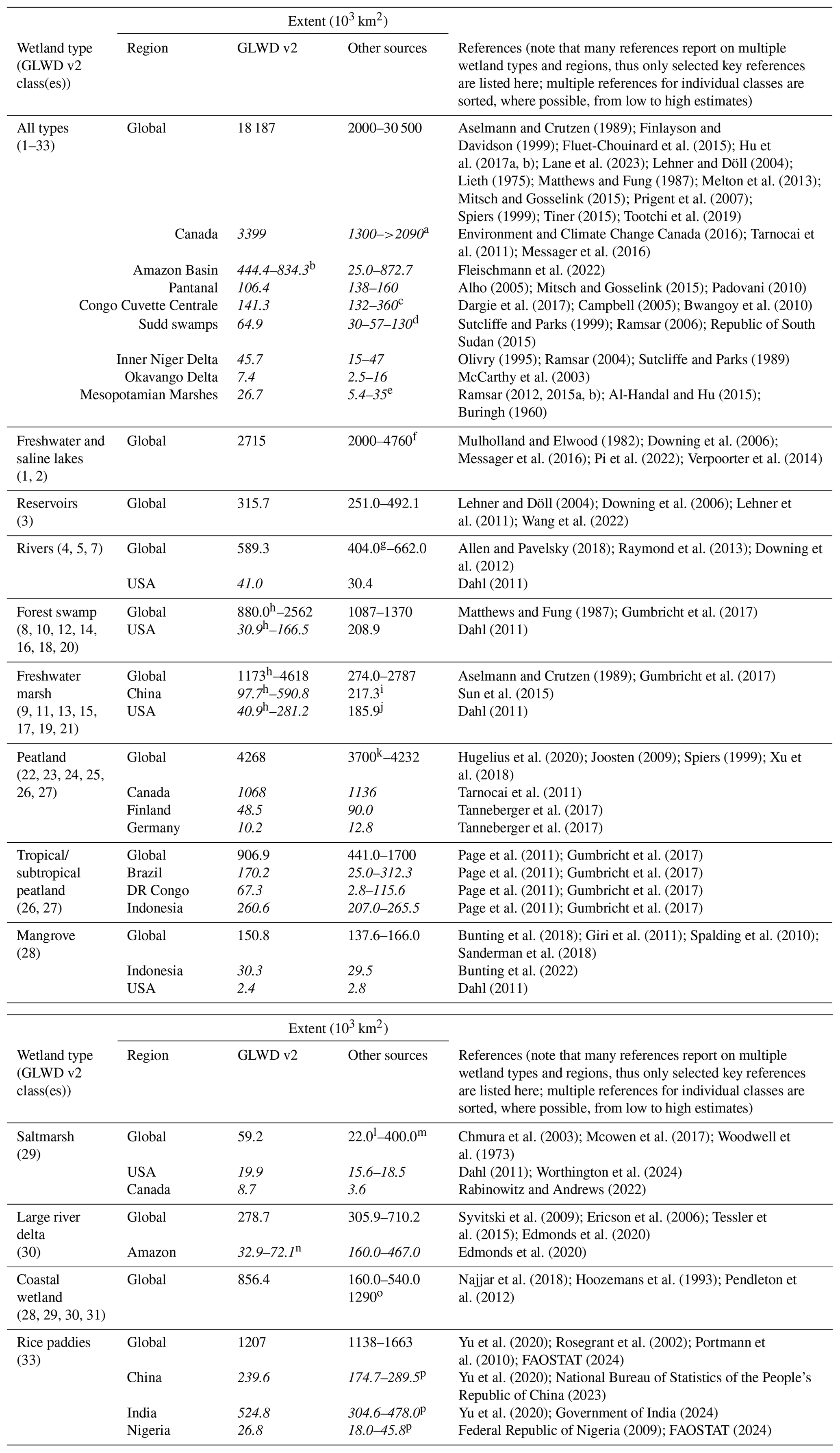
^a Sum of total peatland (Tarnocai et al., 2011) and lake extent (Messager et al., 2016). ^b The low estimate is for lowland floodplains; the high estimate is for entire Amazon Basin. ^c The low estimate is for peatland only; the high estimate includes all (seasonal) wetlands. ^d The low and middle estimates are for permanent and seasonal swamps; the high estimate is for extreme flooding (Republic of South Sudan, 2015). ^e The high estimate is for pre-desiccation marshland extent (i.e., before 1991); the low estimate is for post-desiccation (i.e., start of restoration efforts after 2003). ^f This includes extrapolations to lakes ≥ 1 ha. ^g This is the estimate for rivers wider than 90 m. ^h This is counting only riverine and palustrine classes that are regularly flooded plus the lacustrine class (i.e., classes where flooding is considered to be more permanent). ⁱ This is the estimate for marshes and swamps. ^j This is the estimate for freshwater marshes/wet meadows and shrub wetlands. ^k This is the estimate of northern peatlands only (>23° N latitude). ^l The information is from Chmura et al. (2003), based on inventories from Canada, Europe, Morocco, Tunisia, USA, and South Africa. ^m The information is from Woodwell et al. (1973), extrapolated only from data of the USA and not expecting an accuracy better than ±50 %. ⁿ The low estimate is for class 30 (large river delta) only; the high estimate is for all wetland classes within delta region. ^o The sum of maximum reported extents of mangrove, saltmarsh, and river deltas in previous rows. ^p The high estimate for harvested area, meaning that land cropped for rice multiple times in a year is counted multiple times.

4.3 Comparison to independent data

To assess the robustness of the resulting GLWD v2 wetland maps, we conducted several comparisons and a validation analysis. First, we compared the output of GLWD v2 against independent wetland extents reported in the literature, situating our estimates relative to previous large-scale wetland maps and data compilations. Second, we conducted a validation against ∼ 25 000 global wetland validation samples provided for eight distinct wetland classes. Finally, we cross-compared GLWD v2 against the predecessor map of GLWD v1 and a multi-class satellite-based mapping product at high spatial resolution.

4.3.1 Total area comparisons against literature estimates

Table 4 provides comparisons of GLWD v2 against available global, regional, national, or large individual wetland extent estimates for various wetland types, compiled from >70 literature sources, including field-based surveys, remote sensing analyses, model simulations, expert assessments, meta analyses, and national statistics. The global wetland extent of GLWD v2 (18.2 ×10⁶ km²) lies within the wide range of 2.0 ×10⁶ to 30.5 ×10⁶ km² from literature. In a review of global wetland datasets, Hu et al. (2017a) found that estimates from compilation datasets range between 2.8 ×10⁶ and 12.7 ×10⁶ km² and estimates from remote sensing approaches range between 2.1 ×10⁶ and 17.3 ×10⁶ km². GLWD v2 thus matches the high end of the remote sensing-based estimates. The much larger global wetland extent estimates of 27.5 ×10⁶ and 30.5 ×10⁶ km² produced by Tootchi et al. (2019) and Lane et al. (2023), respectively, are partly explained by the inclusion of model-simulated wetlands that are determined by shallow groundwater occurrences.

The Amazon River basin is a well-studied wetland hotspot and a frequently used benchmark for new wetland maps. The total wetland extent of GLWD v2 for the entire Amazon Basin is 834 300 km², of which 444 400 km² are over lowland floodplains. Fleischmann et al. (2022) compared 29 inundation datasets over lowland regions (elevation <500 m) and estimated the upper bounds of the seasonal minimum and maximum extents as 284 200 and 872 700 km², respectively. The fact that the area of GLWD v2 falls within the range of these independent estimates demonstrates the ability of GLWD v2 to reasonably capture forested and seasonally inundated wetlands in the tropics, some of the most challenging wetland types to detect. The largest spatial discrepancies in this basin occur for interfluvial (or palustrine) wetlands characterized by shallower and more variable rainfall-driven flooding patterns than the more predictable riparian floodplains. To improve the identification of interfluvial wetland ecosystems, more refined efforts may be needed to include additional, small-scale parameters, such as landform (or geomorphic setting) and vegetation (see also Sect. 5.2).

Independent estimates of other large wetland extents across the world, including the Pantanal in South America; the Inner Niger Delta, Sudd swamps, and Okavango Delta in Africa; and the Mesopotamian Marshes in the Middle East also confirm the overall reliable wetland coverage of GLWD v2, consistently near or within the literature estimates that are often wide-ranging (Table 4). One exception to this is the GLWD v2 estimate of 3.4 ×10⁶ km² of wetlands in Canada (34 % of land area), which is more than double the national estimate of 1.3 ×10⁶ km² (13 % of land area; Environment and Climate Change Canada, 2016). This discrepancy is explained by the maximalist perspective of GLWD v2 contrasted with the more restricted national definition. Moreover, the lower national estimate is exceeded by independent peatland and lake area estimates alone (Table 4), demonstrating the discrepancies originating from conflicting definitions and goals. This example underlines the value of GLWD v2 in providing a transparent and spatially explicit baseline of composite wetland extents using fractional cell coverages.

4.3.2 Per-class comparisons against literature estimates

We consider comparisons of individual classes with independent estimates from the literature to be more meaningful in cases where multiple literature estimates converge around a tighter range of values. Therefore, we evaluated GLWD v2 classes by groups tiered by the difference between the maximum and minimum areas found in literature (Table 4): strong agreement (<2-fold discrepancy), moderate agreement (2-3-fold discrepancy), and poor agreement (>3-fold discrepancy).

GLWD v2 classes with strong agreement in literature include reservoirs, rivers, forest swamps, peatlands, mangroves, and rice paddies. Of those classes, all but forest swamps and rice paddies show good agreement between GLWD v2 and global or national independent estimates, with GLWD v2 often falling at the higher end of the reported range. For rice paddy extents, the global area of GLWD v2 agrees well with the global physical area but is closer to harvested area in some countries (accounting for multiple cropping cycles), suggesting either a regional overestimate by GLWD v2 or a potential interannual change in physical area or the type of cropping (see Table 4 for country-level examples). In contrast, GLWD v2 estimates for forest swamps are substantially higher than literature because GLWD v2 broadly defines forest swamps as any inundated area (not otherwise claimed by a different wetland class) with >10 % tree coverage, whereas other definitions of forest swamps also consider more demanding criteria, such as soil moisture and hydrophytic vegetation.

Wetland types with moderate literature agreement include lakes and river deltas. In the case of lakes, discrepancies with literature arise depending on the smallest lake size accounted for, i.e., whether estimates were extrapolated to smaller or even undetectable ponds. GLWD v2 explicitly classifies lakes with a surface area of at least 10 ha, which falls within the range found in literature, and many smaller lakes are expected to be included within the class of other permanent waterbodies. For large river deltas, disagreements in literature estimates about global extents are largely due to the different approaches in delineating the boundaries of deltas from satellite imagery or topographical information, often leading to only coarse outlines of the delta region as a whole. The GLWD v2 estimate for large river deltas is lower than independent estimates in part because we prioritized explicit wetland classes, such as rivers, lakes, and rice paddies, over the generic large river delta class in cases of overlap (e.g., Amazon Delta in Table 4).

Finally, wetland types with poor literature agreement include freshwater marshes, tropical/subtropical peatlands, and saltmarshes. Diverging estimates both within literature and to GLWD v2 are due to multiple issues, including differences in wetland definitions, small wetland occurrences relative to mapping resolutions, difficulties in detection through remote sensors, and sparse and incomplete reporting. Recent methodological improvements have led to larger estimated extents of some classes over time. For example, benefitting from improved remote sensing and field data, tropical peatland complexes in Africa and South America have been mapped to exceed earlier estimates, indicating that previous studies have underestimated their extent. As GLWD v2 incorporates some of the most recent maps of global peatland and saltmarsh extents, it captures a similar total area as referenced in these sources. This also confirms that the multi-step merging process did not cause substantial distortion of original data. Saltmarshes may still be underestimated by GLWD v2 globally, but data quality and completeness varies regionally as shown by the larger saltmarsh areas for the USA and Canada in GLWD v2 compared to literature estimates. The area of freshwater marshes estimated by GLWD v2 is substantially higher than the literature range because GLWD v2 uses freshwater marshes as a catch-all class for all inundated wetlands – not otherwise classified – with sparse vegetation cover (<10 % forest). This goes far beyond the definitions from the literature, which tend to rely on narrower interpretations of vegetation types and soil moisture conditions to identify freshwater marshes (often in ways applicable only to a specific region).

4.3.3 Validation of GLWD v2 against point observations

To validate the resulting maps of GLWD v2, we compared them against a set of global wetland validation samples provided by Zhang et al. (2023) representing point observations for the year 2020. The validation dataset comprises a total of 24 566 sample points located within the land mask of GLWD v2, equally distributed across the world using a stratified random approach and each independently interpreted by five experts with the use of time series optical observations on the Google Earth Engine cloud platform. The samples represent 10 324 non-wetland observations and 14 242 wetland observations, the latter divided into the same eight wetland classes as represented by the GWL_FCS30 global wetland map of Zhang et al. (2023; see Sect. 4.3.5): permanent water, swamp, marsh, flooded flat, saline, mangrove, saltmarsh, and tidal flat.

As the 33 classes of GLWD v2 only partially correspond to the classification system of the validation points, and as GLWD v2 can report multiple fractional wetland classes within each grid cell, no simple one-to-one match with standard omission and commission error calculations is possible. Instead, we first created a confusion matrix that tabulates for each validation class the average fractional wetland extent of each GLWD v2 class, calculated from those grid cells that coincide with a respective validation point (for results, see Table A3 in Appendix A). We then paired groups of GLWD v2 classes that reasonably aligned with the validation classes (see Table A3 for details). For example, this led to grouping all permanent waterbody types (classes 1–6) as permanent water, all forested classes to represent swamp, and all non-forested classes to represent marsh. Because the confusion matrix indicated that validation class saline (which refers to saline soils and halophytic plants along saline lakes) was roughly matched by the saline lake and salt pan, saline/brackish wetland classes of GLWD v2, we combined these two classes while recognizing a potential discrepancy to the validation class definition. For the validation class saltmarsh, the confusion matrix showed the strongest correlations to both the saltmarsh class and the class of other coastal wetlands in GLWD v2, which we therefore grouped together. This misalignment indicates a shortcoming in GLWD v2 of not accurately distinguishing saltmarshes from other coastal wetlands. The validation classes flooded flat and tidal flat have no direct equivalents in GLWD v2 and were thus loosely compared to an amalgamation of all regularly or seasonally flooded classes for flooded flats and to the other coastal wetland and other permanent waterbody classes in GLWD v2 for tidal flats.

Table 5 Accuracy assessment of eight wetland classes from 24 566 wetland validation point samples provided by Zhang et al. (2023) against GLWD v2 class combinations. For the non-standard definition of omission and commission errors as applied here, see main text.

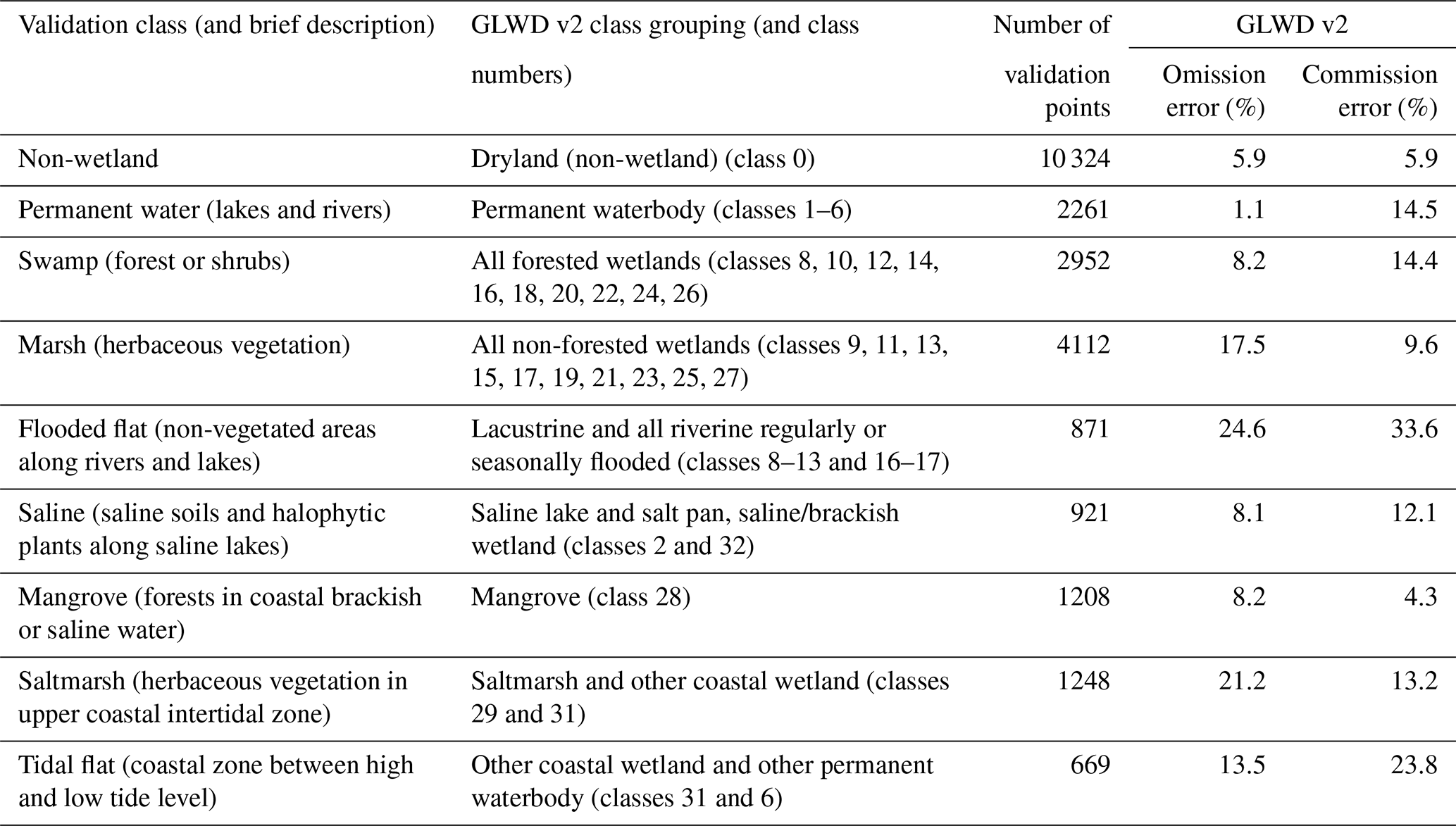
Using these groupings of GLWD v2 classes, we calculated omission and commission errors as follows: an omission error is assumed to exist for GLWD v2 cells that coincide with a validation point but do not contain any fraction of the paired validation class (including the non-wetland class). A commission error is assumed to exist for GLWD v2 cells that coincide with a validation point but do not contain any fraction of the paired validation class (including the non-wetland class), and the cell is covered by at least 50 % of a single validation class grouping that is different from the point's validation class (including the non-wetland class). The latter constraint avoids commission errors for GLWD v2 cells that are occupied only by minority classes or by a majority class that does not relate to any validation class, such as large river delta or rice paddies. It should be noted that despite our attempt to replicate traditional omission and commission error calculations, careful interpretation of the results is advised as fractional classes within the GLWD v2 cells obscure a precise colocation against the validation points.

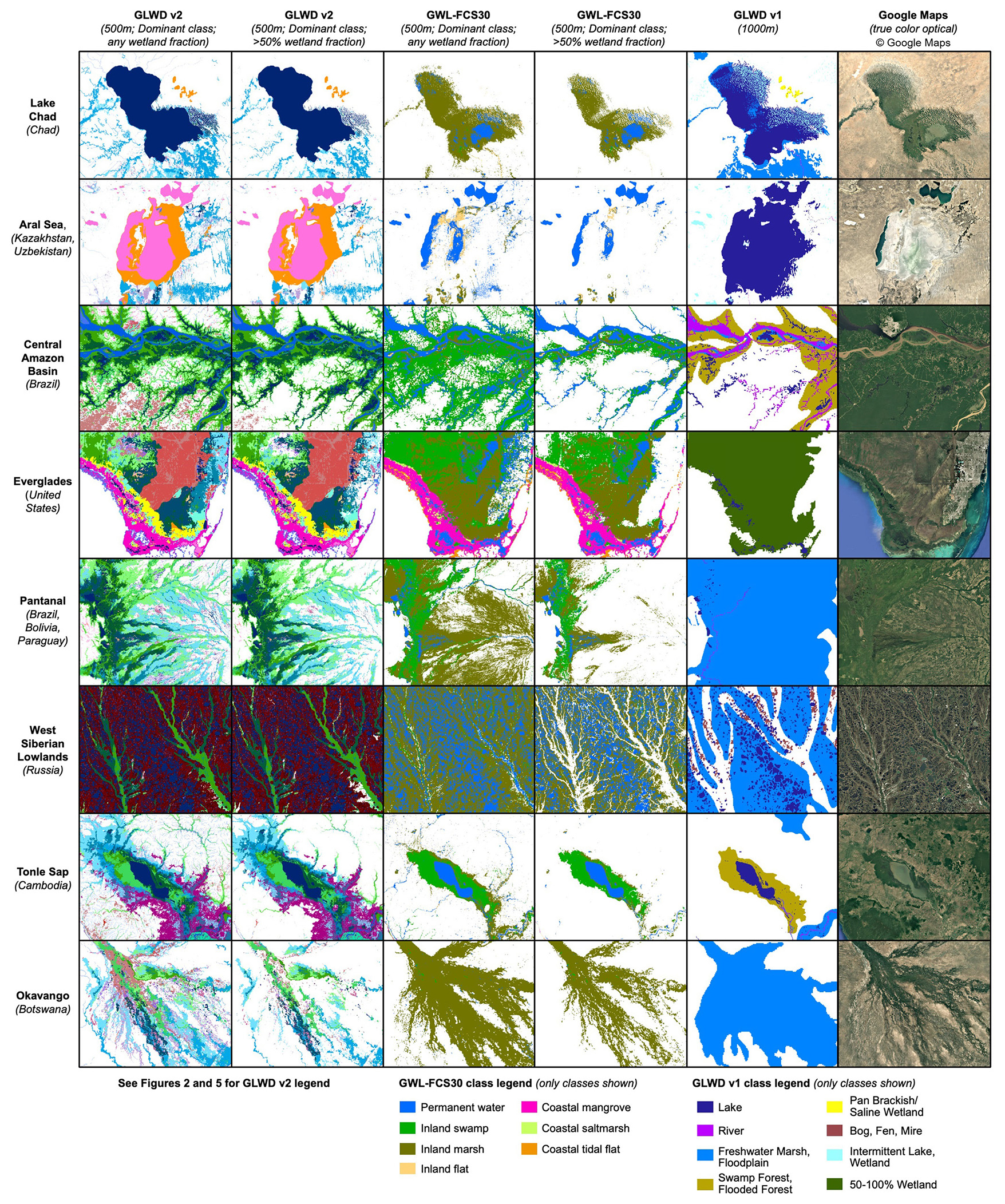
Figure 7 Comparison of GLWD v2, GWL_FCS30, GLWD v1, and optical imagery from © Google Maps over eight globally significant lakes or wetlands. To provide visual comparisons of both class distributions and sub-pixel coverage across datasets, we present the dominant wetland classes per grid cell with two cut-offs of wetland fraction (0 % and 50 %) at a common resolution of 500 m to eliminate misleading optical effects from visualizations at differing scales. However, the spatial aggregation of GWL_FCS30 from its native 30 m resolution understates its precision in wetland delineation, which is unmatched by the other maps in the comparison. GWL_FCS30 data represent the time period of 2000–2020. For a color legend of the GLWD v2 panels, please refer to Figs. 2 and 5.

Following these definitions, we calculated an overall accuracy of 90.5 % between GLWD v2 classes and validation samples, indicating good overall agreement. Omission errors (Table 5) ranged from 1.1 % for permanent water to 24.6 % for flooded flats, the latter likely caused by the inherent mismatch of class definitions. Elevated omission errors for marshes (17.5 %) and saltmarshes (21.2 %) reveal a possible mismatch in class definitions or a limited ability of GLWD v2 to depict these wetland types. Commission errors ranged from 4.3 % for mangroves to 23.8 % for tidal flats and 33.6 % for flooded flats, the latter two again likely due to inconsistent definitions. The commission error for permanent water (14.7 %) can be explained, in part, by historic interpretations of lake extents in GLWD v2, such as the now reduced Aral Sea extent or the fluctuating water area of Lake Chad (see Fig. 7), as well as grid cells dominated by small lakes (mostly in northern latitudes), which may coincide with validation points that mark surrounding patches of marsh, swamp, or upland areas within the cell.

Despite the limited alignment between classification systems and the fractional wetland classes in GLWD v2 which introduce ambiguity in the interpretation, we believe that the validation assessment provides strong support regarding the overall robustness of GLWD v2 results.

4.3.4 Statistical comparison of GLWD v2 against GLWD v1

To demonstrate the progress in upgrading from GLWD v1 to v2, we compared the respective wetland distributions and geographic extents as depicted in the two products. Table A4 (Appendix A) shows the confusion matrix of spatial overlap between classes, and Fig. 7 illustrates select visual examples. At the highest level, i.e., when evaluating the agreement with regards to separating wetlands from non-wetlands, GLWD v1 and v2 reach an overall accuracy of 88.2 %, mostly reflecting the dominant agreement in non-wetland areas. When focusing solely on wetlands, however, only 31.3 % of the combined wetland extents coincide, indicating a rather strong discrepancy in the distribution of wetland areas between the two datasets. This is also confirmed by a modest F₁ score (harmonic mean of precision and recall) of 0.43.

More specifically, GLWD v2 shows an overall omission error across all 12 wetland classes of GLWD v1 of 38.7 %. The highest omission error exists for the intermittent wetland/lake class (74.4 %; Table A4), indicating either high spatial uncertainty in the mostly coarse and generalized delineations of this class in GLWD v1 or a limited ability of GLWD v2 to capture intermittent or ephemeral wetlands at higher resolution. Spatial generalizations in GLWD v1 can also explain why about half of the areas classified either as freshwater marsh/floodplain or as swamp forest/flooded forest are mapped as dryland in GLWD v2. The high omission error for the bog, fen, mire (peatlands) class in GLWD v1 (58.2 %) may be due to the novel representation of peatlands in GLWD v2 as landscape fractions (rather than binary presence/absence), lowering their overall spatial extent in each overlapping grid cell.

In contrast, the lowest omission error exists for salt pan, saline/brackish wetlands (0.1 %), which is not surprising given that this GLWD v1 class was used as an input in the creation of GLWD v2. The lake class in GLWD v1 is well captured by the freshwater lake and saline lake classes from GLWD v2, though 9.6 % of lake surfaces in GLWD v1 are not covered in GLWD v2 by any wetland class. These omissions of lake areas in GLWD v2 – similarly observed for reservoirs and rivers – are mostly caused by known spatial uncertainties in GLWD v1 due to projection issues that introduced substantial misalignments as well as the representation of some reservoirs as circular shapes rather than true shoreline polygons (Lehner and Döll, 2004).

On the other hand, GLWD v2 shows an addition of wetland areas not represented by GLWD v1 that outweighs the omissions, as confirmed by an overall commission error of 61.0 %. Additional wetland extents are due to a combination of (a) new classes that were not mapped in GLWD v1 and (b) a more comprehensive depiction of wetlands in v2. For example, the substantial addition of lake, reservoir and river surfaces as compared to GLWD v1 (see Table A4) can be attributed to the ability of GLWD v2 to represent many smaller waterbodies across various distinct classes. The wetland types in GLWD v2 making the largest spatial additions to GLWD v1 are riverine, seasonally saturated, non-forested and rice paddies followed by arctic/boreal peatland, non-forested and arctic/boreal peatland, forested. These and several other classes have not been explicitly mapped in GLWD v1.

Some GLWD v2 classes (e.g., palustrine wetlands and peatlands) do not have direct equivalents in v1 and can only be evaluated in terms of mixed or partial matches with multiple classes, including overlaps with the indiscriminate fractional wetland classes in GLWD v1. For example, the 0 %–25 % wetlands class of GLWD v1, covering large areas of northern Canada, including the Hudson Bay Lowlands, overlaps with several of the riverine wetland classes in GLWD v2 as well as the two arctic/boreal peatland classes (forested and non-forested), reflecting the refined ability of GLWD v2 to discriminate large wetland complexes into separate ecosystem types. Finally, some mismatches can be explained by regional or class definition issues. For instance, the swamp forest, flooded forest class of GLWD v1 aligns best with the tropical/subtropical peatland, forested class of GLWD v2. This nominal misalignment is caused by the GLWD v1 class only being present over tropical areas, particularly over the Congo Basin.

Our comparison corroborates that GLWD v2 provides an expanded coverage of wetlands compared to GLWD v1 and offers an improved level of separation into distinct classes, especially for riverine and peatland ecosystems as well as rice paddies. Overall, GLWD v1 represents a much more generalized interpretation of global wetland classes (see Fig. 7), underlining the advanced quality and detail of the upgraded GLWD v2.

4.3.5 Visual comparisons of GLWD v2 against a multi-class satellite-based product

Given recent remote sensing advances aiming at detecting and mapping distinct wetland types, we compared GLWD v2 against GWL_FCS30, a global 30 m wetland map with a fine classification system designed for dynamic wetland monitoring (Zhang et al., 2023, 2024). GWL_FCS30 maps eight wetland classes (the same as those of the validation points presented in Sect. 4.3.3) derived from Landsat and other satellite imagery for the time period 2000–2022 and produced by training regional random forest models on sample points generated from select wetland maps. The lack of alignment in class numbers and class definitions between GLWD v2 and GWL_FCS30 (33 classes vs. 8 classes), combined with mismatching resolutions (500 m vs. 30 m) and cell values (fractional classes vs. binary classes), precludes a simple statistical overlay analysis as the colocation of paired GWL_FCS30 wetland classes in the larger GLWD v2 cells remains ambiguous. Besides a basic assessment of overall accuracy, we therefore performed a visual comparison in select wetland regions (Fig. 7). We aggregated the 30 m grid cells of GWL_FCS30 to 500 m resolution and computed the dominant wetland class in each cell in analogy to the dominant wetland class map of GLWD v2. We also masked the 500 m cells where wetlands (from all classes) occupy less than 50 % to compare the fractional cover of wetlands in each product. This approach is intended to focus on the agreement in the distribution of dominant classes in wetland-dense regions. For reference, Fig. 7 also shows depictions of GLWD v1 and optical imagery from Google Maps.

We first assessed the agreement between GLWD v2 and GWL_FCS30 (using GWL_FCS30 data for the year 2020) in their ability to separate wetland from non-wetland cover. The two maps reach an overall agreement of 91.0 %, largely driven by the dominant coverage of upland areas. However, the two sources only agree on 27.7 % of the shared wetland cover. This discrepancy reflects major differences in the respective mapping techniques, definitions, goals, and time periods applied, leading to inherently dissimilar global wetland extents with a total wetland area of 18.2 ×10⁶ km² for GLWD v2 and 6.4 ×10⁶ km² for GWL_FCS30 (for year 2020; Zhang et al., 2023). Despite drawing from the same data sources in some cases, GLWD v2 and GWL_FCS30 can present substantial disparities due to the process of data fusion in GLWD v2 versus sub-sampling to training points and random forest classification in GWL_FCS30. In particular, seasonal wetlands can be missed by remote sensing studies if observations only occur over short time periods.

The visual comparisons shown in Fig. 7 (representing the extended period 2000–2020 for GWL_FCS30) highlight instances of both agreement and disagreement between the maps. High agreement is observed between the permanent water class of GWL_FCS30 and the open water classes of GLWD v2 (classes 1–6). However, differences in the represented time periods can cause significant deviations even for water surfaces that are deemed permanent. For instance, the Aral Sea and Lake Chad show larger open water extents in their long-term depiction of GLWD v2 (including the decade of the 1980s) compared to the more recent observation period of GWL_FCS30 (2000–2020), which shows the two lakes in contracted extents. Mangroves show high agreement between the two maps (e.g., Everglades in Fig. 7), which is expected as both maps used common mangrove datasets as inputs. In contrast, despite similar inputs, lower agreement is observed for the respective saltmarsh classes (not shown in Fig. 7), indicating some confusion with the other coastal wetland class in GLWD v2.

Other examples of Fig. 7 show overall broad agreement between GLWD v2 and GWL_FCS30, yet with notable differences in the delineation of individual classes. In many cases, overall wetland coverage is comparable, but GLWD v2 offers more distinct classes, in particular varying subclasses of riverine, lacustrine, and palustrine wetland types in large river and lake systems (e.g., Amazon, Pantanal, Tonle Sap, and Okavango in Fig. 7). The swamp class of GWL_FCS30 (i.e., forested wetlands) aligns primarily with forested types in GLWD v2, while the marsh class overlaps with both forested and non-forested classes, including forested and non-forested arctic/boreal peatlands in GLWD v2 (e.g., Siberian lowlands in Fig. 7). This misalignment could be caused by disagreements regarding the tree density needed for classification as forested wetlands between the two sources. Overall, caution is recommended when using forested wetland maps as they remain among the most uncertain wetland extents globally.

Despite GLWD v2 presenting a larger overall wetland area and additional classes such as rice paddies, it omits some areas that are classified as swamp and marsh by GWL_FCS30, indicating specific gaps in GLWD v2. Visual inspections suggest that marsh areas can extend beyond the edges of peatlands in GLWD v2. These marshes are dispersed geographically and are particularly clustered in northern latitudes. Similarly, some missing swamp areas appear to capture minor wetland complexes in tropical regions omitted by GLWD v2, often near the edge of river deltas and coastlines.

In conclusion, there are both areas of agreement and disagreement between the two maps. Nonetheless, given their different classification systems, they display overall reasonable levels of concurrence. Considering the higher spatial resolution of GWL_FCS30 and its ability for short-term updates, as well as the more refined classification and longer-term vision of GLWD v2, these two products demonstrate the substantial opportunities that exist for combining different mapping approaches as a step towards dynamic remote sensing products of wetland classes in the future.

5 Discussion

GLWD v2 provides a comprehensive representation of the world's wetland ecosystems by harmonizing state-of-the-art data sources at grid cell resolutions ranging from ∼ 10 m to 1 km into a target resolution of 500 m. By drawing on global or near-global inputs, 33 individual wetland classes were mapped consistently across the world, avoiding regional discrepancies that can emerge from a patchwork of regional or national data sources. The 33 resulting classes of GLWD v2 improve upon previously available maps, including GLWD v1. By design, GLWD v2 aims to address the call for consistency and integration in global surface water mapping (Rajib et al., 2024) and to help in closing the gap between field inventory typologies and globally applicable classifications (Davidson et al., 2018).

5.1 All-inclusive wetland definition and applied criteria

The compilation of GLWD v2 was carried out with the objective of including all wetlands at their maximum extent rather than enforcing strict wetland type definitions. As a result, each wetland type is determined by a distinct set of criteria, resulting from the approaches and constraints of the original data sources, rather than a single harmonized definition. Different wetland classes were specified by a combination of spatial, temporal, and ancillary characteristics and can be grouped into three broad categories: waterbodies, other inland wetlands, and other coastal wetlands (Fig. 2). Aside from the exceptions described in the Methods section, the following general class characterizations can be distilled from our data fusion procedures and merger rules:

• Waterbodies comprise open water surfaces wider than 30 m for rivers and larger than 10 ha for lakes. Areas of small streams were predicted statistically for those exceeding 0.1 m³ s⁻¹ (100 L s⁻¹) in average flow or 10 km² in catchment size. Waterbodies generally have persistent presence of open water surfaces; however, specific waterbody types may not be fully inundated at all times. For example, the reservoir polygons may delineate surfaces at high water levels, the rivers may encompass multiple shifting channels, and a substantial number of small streams will experience intermittent flow. Other permanent waterbodies include, but are not differentiated for, additional parts of rivers, small lakes, ponds, and artificial water surfaces such as canals, as long as they exceed 30 m in width, which reflects the detection limit of the used optical imagery.

• Other inland wetlands represent either periodically inundated or surface-saturated areas of various frequencies, with or without forest cover, or represent organic peatland soils, rice paddies, or salt pans.

• Other coastal wetlands are defined by either a particular vegetation cover or collectively as wetlands located less than 10 m above sea level and connected to the coastline as these criteria were used across several of the data sources or were introduced during the data fusion process.

The broad wetland definition of GLWD v2 allows it to encompass most national definitions, except for specific wetland types that cannot be reliably mapped globally (e.g., explicit identification of aquaculture ponds, or presence of subterranean or geothermal wetlands). Setting aside missing classes, GLWD v2 may still underrepresent wetland extents due to the detection size and revisit period of observation systems but not due to restrictions derived from definitions. With its broad wetland definition, GLWD v2 aims to address the widely shared concern that published global wetland extent estimates from either national inventories or remote sensing technology may still underestimate the true global wetland extent (Davidson et al., 2018).

5.2 Classification design and relationship to existing classification systems

The multiple factors used to categorize wetland types – including hydrology, inundation, soils, vegetation, landscape position, and connectivity – allow GLWD v2 to represent a wide variety of wetland conditions while filling the need for a generalized and manageable classification system. In particular, the inclusion of criteria beyond inundation, such as vegetation and soil conditions, more closely aligns GLWD v2 with field-based and national classifications and inventories (Ramsar Convention on Wetlands, 2002; Gerbeaux et al., 2018; Junk, 2024). In certain regions, GLWD v2 reaches a level of detail comparable to national and regional classification schemes.

GLWD v2 does not follow a strictly hierarchical classification approach with one specific criterion for subdivisions at each level. Such an approach would yield a much larger number of subclasses. Instead, our grouping of classes into a simplified and systematic but versatile classification system (Fig. 2) allows users to combine classes in various ways for applications where fewer and/or broader classes are more useful. For instance, regrouping of classes can occur along various axes, including open water vs. vegetated, inundated vs. saturated, forested vs. non-forested, connected to waterbodies vs. isolated, or mineral vs. organic soils.

The design of GLWD v2 classes stemmed from two primary methodological procedures: first, we harmonized existing maps of explicit wetland types. In this process, we selected one representative dataset per class (e.g., one river dataset) wherever possible to reduce the issue of double counting or temporal mismatches for overlapping water features. Second, once all pre-defined classes were harmonized, we classified the extent of indiscriminate inundation by attaching hierarchical labels. This classification of indiscriminate inundation incorporates ideas from several classification schemes. We elected to combine components of the “landscape position, landform, water flow path and waterbody type (LLWW) descriptors” (Tiner, 2014) along with simple biotic discriminants (forested vs. non-forested). The classification in GLWD v2 diverges from proposed hydro-geomorphic wetland classification schemes (e.g., Brinson, 1993; Semeniuk and Semeniuk, 1995) by not including landform (slope, channel, depression, etc.) among its criteria, not least due to the lack of high-precision input data to determine small-scale geomorphic features. Instead, GLWD v2 uses inundation and saturation frequency as well as spatial connectivity between wetland ecosystems via contiguous surface water extents as a proxy for hydrological, biogeochemical, and ecological connectivity. This is also why inundation extents and frequencies from GIEMS-D3 and the CaMa-Flood hydrological model were chosen as inputs over purely topographical definitions of floodplains such as those produced by Tootchi et al. (2019) and Lane et al. (2023).

Table 6 Class equivalency between GLWD v2 and common global wetland typologies: the wetland and deep-water classification of the US National Wetlands Inventory (NWI) (Cowardin et al., 1979), the classification of the Ramsar Convention on Wetlands, the simplified Ramsar types of the Global Wetland Outlook (GWO) (Davidson and Finlayson, 2018), and the IUCN global ecosystem functional groups (EFGs) (Keith et al., 2022). Classes listed on the same row signify partial equivalence, ranging from incomplete overlap to complete nestedness. Additional class overlaps are possible depending on application and we recommend case-by-case re-evaluation of this crosswalk. Some classes from Ramsar, GWO and NWI are not listed on the table because of the absence of an equivalent class in GLWD v2. Class names were modified for brevity.

Although GLWD v2 presents a novel classification scheme, its typology shares basic similarities with some of the most common classification systems, including those of the ecosystem functional groups (EFGs) of the International Union for Conservation of Nature (IUCN) (Keith et al., 2022), the US National Wetlands Inventory (Cowardin et al., 1979), and the Ramsar Convention on Wetlands (Table 6). Although classes rarely have one-to-one equivalencies, several comparable groupings emerge. GLWD v2 is less detailed than IUCN's EFGs for waterbodies but offers more levels of separation for other freshwater wetlands (28 EFGs qualify as wetlands). To increase concordance with the IUCN system and facilitate potential crosswalks of classifications, the simplified representation of rivers and lakes in GLWD v2 could be further expanded by employing ancillary datasets for river types (e.g., the Global River Classification, GloRiC; Ouellet Dallaire et al., 2019) and lake characteristics (e.g., LakeATLAS; Lehner et al., 2022). An analogous division into bioclimatic regions as proposed in the IUCN typology (e.g., tropical, temperate, and alpine) could also be added to GLWD v2.

GLWD v2 generally aligns well and shares nomenclature with the system and subsystem levels of the US National Wetlands Inventory (hereafter NWI; Cowardin et al., 1979; Cowardin and Golet, 1995), a classification of wetlands and deep-water habitats used by the US Fish and Wildlife Service. Comparing higher levels of classification hierarchy, GLWD v2 applies its landscape connectivity labels (lacustrine, riverine, or coastal) far more broadly than NWI does, as GLWD v2 is inspired by the LLWW approach. At the lower levels of classification, GLWD v2 follows a vegetation dichotomy similar to the more numerous modifiers used by NWI (e.g., vegetation, soil, sediment). Finally, the Ramsar Convention's classification, which was gradually expanded over time to accommodate the diversity of the world's wetlands and later simplified in the Global Wetland Outlook (Davidson and Finlayson, 2018), covers a similarly large breadth of wetlands as GLWD v2. However, the ambiguity and overlap between some of the Ramsar class definitions (Semeniuk and Semeniuk, 1997; Finlayson, 2016) present relatively few direct equivalencies with GLWD v2 wetland classes.

5.3 Limitations and uncertainties

Our validation and comparison assessments (Sect. 4.3) confirm an overall reasonable wetland representation of GLWD v2, at both global and regional scales. However, differences in wetland definitions and the intrinsic temporal (both interannual and intra-annual) variability of wetland extents can lead to vast discrepancies and preclude any reliable one-to-one comparison. For example, in our validation against global wetland samples the condensed eight wetland classes of the observation dataset do not directly align with our approach or outputs, and our applied class aggregations only partially match the validation classes. The reported omission and commission errors and overall accuracy therefore encompass an ambiguous mix of detection limitations and incompatible wetland definitions, rendering a detailed interpretation of the achieved quality of GLWD v2 difficult.

The general reliability of the different GLWD v2 classes depends on both their respective data sources and subsequent data manipulation and interpretation steps. As a composite mapping product, GLWD v2 inherits the uncertainties and shortcomings of its data sources. Given the large diversity of input datasets, we offer only brief summaries of key limitations in Table 1 but refrain from discussing the quality of each source in more detail; instead, we refer the reader to the original publications of the source datasets (see Table 1). Overall, the recent growth of optical imagery archives has resulted in high-quality maps of inland surface water, including lakes and rivers, that were directly incorporated into GLWD v2 without substantial alteration. Certain explicit wetland types, such as mangroves and saltmarshes, were available as detailed maps requiring only limited modifications, whereas other classes, such as peatlands or rice paddies, were derived from coarser historical maps or synthesized from multiple input maps. The most challenging wetland types to delineate were those based broadly on connectivity and flood frequency assessments, including lacustrine, riverine, palustrine, and coastal wetlands with varying recurrence intervals of inundation or saturation. These wetland types were mapped from indiscriminate, coarse-resolution multi-sensor estimates spanning over 2 decades, which were downscaled using topography information and then combined with ancillary data to differentiate individual wetland classes. Given the increased complexity in this process and the reliance on expert decisions, these ecosystem types are expected to exhibit higher levels of uncertainty.

Despite our efforts to avoid or reduce double counting of wetland surfaces and minimize uncertainties stemming from the fusion of diverse inputs, we acknowledge that such uncertainties, distortions, and overestimations likely exist in GLWD v2, especially at local scales and in areas where multiple source datasets overlap. For example, temporal misalignment between water and wetland features is expected across multiple data sources due to, for example, migrating channels or shifting littoral edges, which can lead to erroneous overestimations of total water surfaces when merged (by summation) into a static product. Spatial or temporal overestimations may also be caused by projection issues, leading to false offsets of waterbody features in multiple overlapping sources; by the insufficient resolution of some source datasets (e.g., by interpreting small wetland patches to cover an entire cell); or by the preferential use of wet periods when mapping wetland extents. Substantial local mismatches are expected between the data sources used for arctic/boreal, temperate, and tropical/subtropical peatlands due to differences in their definition of soil organic content and horizon depth as well as the accuracy of their distribution. Nonetheless, our comparisons of GLWD v2 to other datasets (Sect. 4.3) suggest that these uncertainties are neither systematic nor sufficiently large to deviate from most literature estimates. The process of synthesizing multiple data sources through masking, merging, and compositing is essential to produce a comprehensive and coherent map with spatially explicit distinctions between classes, especially given the many different types of wetlands on Earth. However, our harmonization of input sources does not improve upon their individual qualities; hence, the original datasets at their native resolutions remain the best sources for specific wetland types.

To be applicable globally, the typology of GLWD v2 simplifies distinctions of certain wetland types while also emphasizing globally observable characteristics. For example, we excluded or used proxy measures for field-level indicators that are not directly observable from space, such as water table depth, hydrophytic vegetation, soil condition, microtopography, bathymetry, and salinity (Tiner, 2016; Gallant, 2015). Similarly, plant productivity and nutrient status of wetland ecosystems are used in some national classifications (e.g., ombrotrophic bog vs. minerotrophic fen in the Canadian classification) but are not applicable globally due to missing information at the necessary level of detail to achieve a reliable discrimination. Moreover, these local key characteristics are of secondary importance to the dominant drivers of wetland condition at the global scale that we used for GLWD v2 (hydrology, vegetation, soil type, and landscape position).

The implementation of landscape position, inundation frequency, and surface connectivity between waterbodies and other wetlands required some notable simplifications that have caused GLWD v2 to deviate from more detailed inventories. First, the separation of coastal wetlands is based on connectivity to the marine coast, which is only a proxy for water salinity or tidal hydrodynamics. This may explain some of the observed confusion of the saltmarsh and other coastal wetland classes (see Sect. 4.3). Second, lacustrine or riverine wetland types were labeled based on surface water connectivity to nearby lakes or rivers, but we did not seek to further separate wetlands fed by groundwater (Tootchi et al., 2019) or local runoff and rainfall (Fan and Miguez-Macho, 2011). Third, palustrine wetland types were intended to represent geographically isolated wetlands, but some can remain connected with waterbodies through subsurface flow (Cohen et al., 2016). Fourth, surface inundation and saturation as depicted in our source datasets ignores non-saturated wet soil conditions, which, if added, may provide further paths of connectivity. Finally, the applied distance thresholds and methodological assumptions used to determine and further stratify the connectivity-based classes using inundation frequencies were determined by expert judgment. This approach, though guided by visual calibration against known wetland complexes, is prone to subjectivity and ambiguity. Overall, we expect that the subclass distinctions derived from the landscape position, connectivity, and flood frequency analyses are the most uncertain within GLWD v2, and caution should be exercised in applications that rely on their individual characteristics.

Rather than being a time-resolved product, GLWD v2 depicts contemporary conditions and limited aspects of inundation periodicity (seasonal, ephemeral, etc.) as a static map. We argue that a static wetland representation is appropriate to determine the overall extent of wetland ecosystems given that seasonal, annual, or even decadal wetting and drying cycles are part of the ecological condition of a wetland (i.e., the wetland still exists if it is in a naturally drier phase or a dry state). However, the lack of dynamic, time-resolved information in GLWD v2 precludes a more refined classification and definition of wetland boundaries, such as by delimiting wetlands at their average maximum extent over a specified time period (e.g., as proposed by Junk, 2024). Therefore, GLWD v2 offers only limited utility for applications that require the analysis of dynamic wetland states. Furthermore, the static wetland depiction of GLWD v2 represents a long-term baseline centered around the contemporary period of 1984 to 2020 and should not be used to directly infer or monitor trends over time in global wetland distribution. Some input sources are limited to data without explicit temporality, and despite our best efforts to align associated time periods, there remain unresolved mismatches between sources due to different temporal snapshots (see Table 1) or time-integrated summaries (e.g., flood frequencies). While desirable, a time-resolved version of GLWD v2 at regular intervals would require both a narrower selection of data sources and more lenient assumptions about wetland classes to conform with data limitations. Moreover, temporal representation presents new challenges, such as the high uncertainties of transitional wetland systems that fluctuate between saline, brackish, and freshwater types as salinity levels change in response to flooding or drying cycles. Overall, interannual variation in seasonally flooded areas is likely the norm rather than the exception, as exemplified by the analyses of Amazon floodplains (Fleischmann et al., 2022).

5.4 Future of mapping wetland ecosystems globally

For continuous monitoring of different wetland types to be achieved, high-resolution remote sensing paired with novel modeling approaches and/or machine learning techniques is needed (e.g., Gallant, 2015; Murray et al., 2022; Bunting et al., 2023). Ideally, such efforts should be supported by wide networks of water level loggers adequately capturing the variety of wetlands across the world. With new satellite missions, such as SWOT and NISAR, GLWD v2 may act as a baseline layer and offer a globally applicable classification system onto which new data streams can be added to evaluate decadal-scale changes (Biancamaria et al., 2016). In the future, harmonization of GLWD v2 with time series information derived from Landsat and/or Sentinel (rivers, lakes, and other permanent surface water) and additional sources such as multi-satellite inundation products could form the backbone of a temporally dynamic representation of wetland ecosystems.

Improvements in spaceborne hydrology observations represent a key component to develop an enhanced approach to detect, classify, and monitor wetlands globally. Dependable estimates of soil surface moisture, sub-canopy inundation, refined topographic data and detection of hydrophytic vegetation would allow for more detailed and reliable class distinctions. Furthermore, the GLWD v2 classification could be expanded by adding labels to waterbodies based on their surroundings, leading to new classes such as peatland lakes or floodplain lakes. Finally, the exploration of a hydro-geomorphic classification could be ideal for functional assessments of wetland ecosystem types and the services they provide (Semeniuk and Semeniuk, 1995, 2011; Davis et al., 2013).

6 Data availability

The GLWD v2.0 database, as presented in this paper, is available under a CC-BY 4.0 license at https://www.hydrosheds.org/products/glwd (last access: 1 May 2025) and a copy has been deposited on the figshare data repository at https://doi.org/10.6084/m9.figshare.28519994 (Lehner et al., 2025). The data layers are provided in different formats and are accompanied by technical documentation explaining file names and specifications.

7 Conclusions

GLWD v2 synthesizes the best available maps and Earth observation data from the last ∼ 30 years into a coherent typology of the world's wetland ecosystems. The resulting 33 wetland types substantially narrow the gap between field-level classification systems designed for local monitoring or management and globally applicable classifications informing large-scale conservation strategies, Earth system modeling, and international policymaking. GLWD v2 provides gridded global maps of dominant wetland classes and fractional cell coverage of each class at 500 m resolution to enable a new generation of research and applications. In particular, the design of GLWD v2 as a set of 33 individual but complementary wetland layers is expected to facilitate the study of specific wetlands of interest while remaining consistent with the total global wetland extent and distribution. As a comprehensive static wetland map of contemporary (∼ 1984–2020) wetlands generated from satellite and ancillary data, GLWD v2 is an important step in the transition of wetland monitoring from a compilation task to a continuous observation process.

If coupled with time series information from novel remote sensing technologies, GLWD v2 can provide a foundation to transition towards a monitoring system capable of evaluating trends and variations of individual wetland types. Until that time, GLWD v2 provides an important baseline of wetland extent and classification that can facilitate the derivation of indicators for tracking progress towards the UN Sustainable Development Goal 6.6 of protecting water-related ecosystems. Given the importance of wetlands at the nexus of water, climate, and biodiversity, the dataset can also inform international policy frameworks, such as the Convention on Biological Diversity (CBD), the Convention on Migratory Species (CMS), the Intergovernmental Science-Policy Platform on Biodiversity and Ecosystem Services (IPBES), the Ramsar Convention on Wetlands, and the United Nations Framework Convention on Climate Change (UNFCCC).

Appendix A: Additional tables

Table A1 Description of data sources shown in Fig. 1. Temporal resolutions without recurrence interval are separated into categorical and static according to whether information on inundation frequency is represented in the classification.

Table A2 Further information on each literature reference and its related data source(s) used in the comparisons shown in Table 4. Data sources include field-based surveys, remote sensing products, expert assessments, meta analyses, and national statistics.

Table A3 Confusion matrix showing average fractional grid cell area (percent) of GLWD v2 classes at the location of 24 566 wetland validation samples provided by Zhang et al. (2023). Given the lack of direct equivalencies between the two classification systems, correlations between pairs of individual classes are not as informative as comparisons between groups of classes (e.g., combined waterbody classes 1–6 of GLWD v2 best represent the permanent water class of the validation points). The GLWD v2 classes highlighted in bold in each column represent the group combinations that were used to match the validation classes and to compute omission/commission rates and accuracy indices in Sect. 4.3.3 and Table 5.

Table A4 Confusion matrix showing fractional grid cell area (in 10³ km²) of GLWD v2 classes located in each GLWD v1 class (at 500 m cell resolution). The overlap was performed by first disaggregating GLWD v1 from 1 km (30 arcsec) to 500 m (15 arcsec) resolution and then intersecting it with the fractional wetland area from GLWD v2, using the land mask definition of GLWD v2.

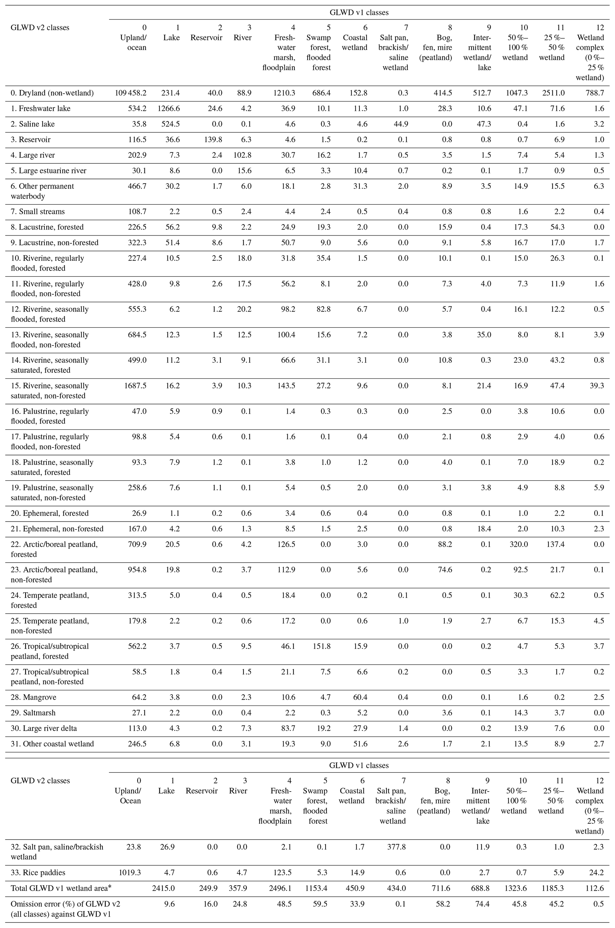
^* Calculated at the middle of the range for fractional classes no. 10, 11, and 12, i.e., 75 % for class 50 %–100 %, 37.5 % for class 25 %–50 %, and 12.5 % for class 0 %–25 %.

Appendix B: Additional figures

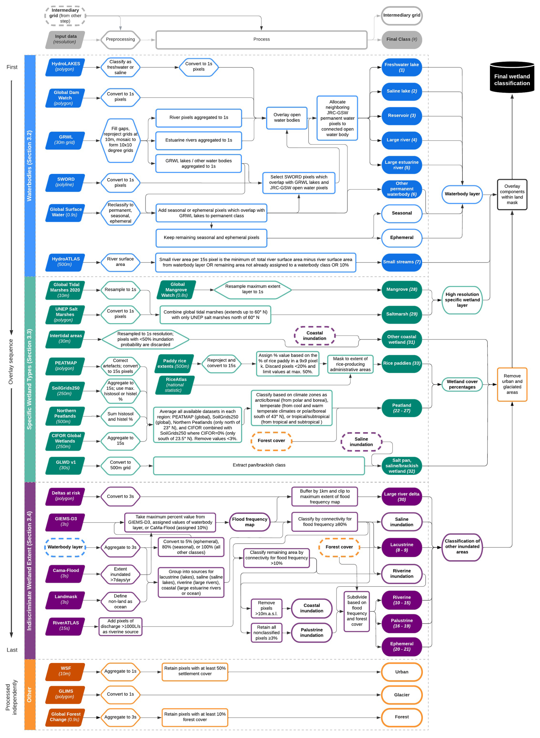
Figure B1 Detailed schematic of the workflow and processing steps to create GLWD v2, expanding on Fig. 3 in the main text. The processing steps are grouped into three main sections, corresponding to Sect. 3.2 (top, blue), 3.3 (middle, green), and 3.4 (bottom, purple) of the main text. Additional (non-wetland) layers are shown in orange, and a diagram legend is shown in light grey at the top of the figure. This schematic aims to indicate, from top to bottom, the sequential order of insertion of different datasets. In some cases, steps from earlier or later sections of the diagram are used as inputs, as indicated with dashed outlines. From left to right, the schematic describes the input datasets, data preprocessing, main processing steps, and output raster maps of each class (or group of classes). This schematic aims to describe the processing steps of GLWD v2 in high detail while maintaining legibility in a visual format. More specific descriptions of individual steps can be found in the main text in Sect. 3.2–3.4.