Discrete global grid system flow routing datasets in the Amazon and Yukon basins

Discrete global grid systems (DGGS) are emerging spatial data structures widely used to organize geospatial datasets across scales. While DGGS have found applications in various scientific disciplines, including atmospheric science and ecology, their integration into physically based hydrological models and Earth system models (ESMs) has been hindered by the lack of flow routing datasets based on DGGS. In response to this gap, this study pioneers the development of new flow routing datasets using icosahedral Snyder equal-area (ISEA) DGGS and a novel mesh-independent flow direction model. We present flow routing datasets for two large basins, the tropical Amazon River basin and the Arctic Yukon River basin. These datasets (1) facilitate the adoption of DGGS for hydrological models and (2) provide flow routing inputs for evaluation of DGGS-based flow routing in the Amazon and Yukon river basins. The data are available at https://doi.org/10.5281/zenodo.8377765 (Liao, 2023).

1 Introduction

Discrete global grid systems (DGGS) are emerging spatial data models that use hierarchical tessellations of cells to partition and address Earth's surface. DGGS have been widely adopted as a standard data fabric to organize geospatial datasets across various granularities (Goodchild, 1994; Kimerling et al., 1999; Sahr, 2024; Purss et al., 2016). DGGS, such as the icosahedral Snyder equal-area (ISEA) Aperture 3 Hexagon (3H), are used in many disciplines, including the Geographic Information System (GIS) (Sahr, 2019), hydrology (Li et al., 2022), atmospheric science (Randall et al., 2002), and ecology (Ellis et al., 2021; Mechenich and Žliobaitė, 2023). However, DGGS have seen limited adoption in physically based, spatially distributed hydrological models and Earth system models (ESMs) (Li et al., 2022), mainly because ready-for-use flow routing datasets based on DGGS are unavailable.

Flow routing datasets are essential for spatially distributed hydrological models, and they typically rely on two data model paradigms. The first one is the rectangular mesh-based grids, also known as rasters (Esri Water Resources Team, 2011; Wu et al., 2012). This method often requires high-quality digital elevation model (DEM) rasters such as METIR hydro (Yamazaki et al., 2019; Amatulli et al., 2022). It is also subject to several other limitations, including the challenge of coupling with other unstructured mesh-based numerical models. The second one is the vector-based polylines (Lin et al., 2021), which are often produced through the combination of high-resolution raster-based and remote sensing product methods. However, these polylines often contain various artifacts, including disconnected segments, and thus they cannot be used directly across different spatial scales (Huang and Frimpong, 2016). Another limitation of this method is the lack of communication between the river and its adjacent riparian zones.

We recently pioneered the ability to generate flow routing datasets using unstructured Model for Prediction Across Scales (MPAS) meshes (Engwirda and Liao, 2021; Liao et al., 2023b). Although MPAS meshes have gained traction in the oceanographic and atmospheric modeling communities, DGGS meshes are also widely adopted across the Earth sciences and GIS communities. To date, there are no available DGGS-based flow routing datasets that include flow direction information. This is because existing DGGS-based hydrology datasets are often derived by resampling from existing raster-based datasets, which does not support vector-based datasets such as flow direction (Chaudhuri et al., 2021). In addition, most traditional flow direction models in various GIS software packages only support raster datasets. This highlights the need for a method to natively generate flow direction datasets within a DGGS-based framework.

Compared to structured rectangular meshes, including latitude–longitude geographic coordinate systems (GCS) and projected coordinate systems, DGGS have several advantages. These include (1) better spatial coverage and consistent spatial resolution for the high latitudes (Liao et al., 2020), (2) potential numerical performance improvement for coupled surface and subsurface hydrological models (Liao et al., 2022), and (3) more flexibility in spatial resolution due to their hierarchical data structure. Specifically, the ISEA DGGS projection stands out for its benefits to hydrological models and ESMs. As an equal-area icosahedral DGGS projection, ISEA eliminates the need for equal-area projection. In addition, the hexagonal grid geometry resolves ambiguity among cell neighborhoods by ensuring uniform adjacency, thereby offering significant advantages in the domain of hydrology.

This study breaks new ground by developing new flow routing datasets using the ISEA3H DGGS and our innovative mesh-independent flow direction model. We present flow routing datasets for the Amazon and Yukon basins, which are among the world's largest river basins in the tropics and Arctic, respectively, and play important roles in the local, regional, and global climate and ecosystems. These datasets can (1) facilitate the adoption of DGGS for hydrological model development and (2) provide flow routing inputs for evaluating DGGS-based flow routing in the Amazon and Yukon river basins.

2 Method

A list of datasets and models used in our workflow to produce DGGS-based flow routing datasets is depicted in Fig. 1.

Figure 1 Workflow diagram demonstrating the DGGS-based flow routing dataset generation process using three steps (dashed boxes). Step 1: river network simplification using REACH. Step 2: DGGS mesh generation using DGGRID. Step 3: flow direction modeling using HexWatershed (including PyFlowline). The brown boxes are user-provided datasets. The orange boxes are intermediate results (e.g., conceptual river networks modeled by PyFlowline). The light-green box is the final data product.

We first introduce the input datasets used in each step and then the models used. Additional information is provided in the Supplement.

2.1 Input datasets

2.1.1 Vector river networks

The vector river network datasets of the Amazon and Yukon basins were obtained from the HydroSHEDS database (Lehner et al., 2008). The HydroSHEDS v1 dataset is derived primarily based on elevation data obtained in 2000 by the United States National Aeronautics and Space Administration (NASA) Shuttle Radar Topography Mission (SRTM). Specifically, we obtained the HydroRiver datasets of South America and the Arctic (https://www.hydrosheds.org/products/hydrorivers, last access: 25 September 2023). While HydroSHEDS products, including the river networks, may not provide the highest level of accuracy in depicting river and basin maps, they are widely acknowledged and evaluated for applications at regional and global scales. These datasets are used in Step 1.

2.1.2 Vector watershed boundary

The vector Amazon basin boundary was obtained through NASA's Oak Ridge National Laboratory (ORNL) Distributed Active Archive Center (DAAC) (Mayorga et al., 2012). The vector Yukon basin boundary was obtained through HydroBASINS, which is part of the HydroSHEDS product. These datasets are used in Step 2.

2.1.3 Raster terrain datasets

High-spatial-resolution DEM datasets of the Amazon basin at 30 arcsec (∼1 km at the Equator) were obtained through NASA's ORNL DAAC (Saatchi, 2013). Similar to HydroSHEDS, this DEM was produced as a subset of the SRTM DEM. The flow accumulation and length datasets at the same spatial resolution are used for data validation. Similarly, void-filled DEMs and flow accumulation datasets of the Yukon basin at 15 arcsec (∼ 500 m at the Equator, ∼ 250 m in Alaska) resolution were obtained from HydroSHEDS. These datasets are used in Step 3.

2.2 Models

Our workflow primarily leverages three software models to produce the DGGS-based flow routing datasets. The models are run in sequence in three steps: (1) the REACH model preprocesses the vector river networks, i.e., HydroSHEDS, to produce the simplified river networks; (2) the DGGRID model generates the DGGS mesh using the basin boundaries; and (3) the HexWatershed model generates the flow routing datasets using outputs from Steps 1 and 2. Descriptions of each model and step are provided below.

2.2.1 HydroSHEDS river network simplification using REACH

Because the full HydroSHEDS river network dataset contains millions of river channels that range between a few and thousands of kilometers, they cannot be represented equally in hydrological and Earth system models. For example, any river channel less than 10 km in length cannot be represented well if the mesh cell resolution (in length) is also 10 km. To address this challenge, we used the REACH library (Engwirda, 2023) to preprocess (simplify) the HydroSHEDS river network. In this step, only major river channels and tributaries resolvable at scales of interest are preserved. REACH employs a greedy network simplification algorithm in which the maximal set of river reaches is processed in priority order of increasing upstream catchment area. River reaches are removed incrementally if they meet the following criteria: (1) their length is shorter than a user-defined tolerance or (2) they are geometrically closer to another higher-priority reach segment than a user-defined tolerance. Upon removal of a given river reach, the downstream network is simplified – merging any newly contiguous segments into “super reaches” and updating their associated priorities. While heuristic in nature, this greedy approach leads to simplified river vector networks that are appropriate for both hydrological analysis and unstructured mesh generation, with the network pruned in a least-catchment-area-first manner. This retains hydrologically important reaches while removing geometrical features smaller than the desired mesh scale to ensure compatibility between the flow network and the computational grid.

The user-defined tolerance is a measure of how much detail the mesh should preserve and distinguish between river channels because a mesh cell conceptually can only represent one main channel unless it is a river confluence. In practice, the user-defined tolerance is often set as the mesh cell's spatial resolution (in length), which can vary in space as well. In this study, because we use four resolution levels from the DGGRID model to generate the flow routing datasets, the corresponding resolutions in length (square root of the area) are used as the user-defined tolerance parameters (Table 1).

Table 1 The DGGRID mesh generation resolutions used to produce the flow routing datasets for the Amazon and Yukon basins. These resolutions are chosen to accommodate major existing large-scale hydrological and Earth system models. The level-14 resolution is only used for mesh generation.

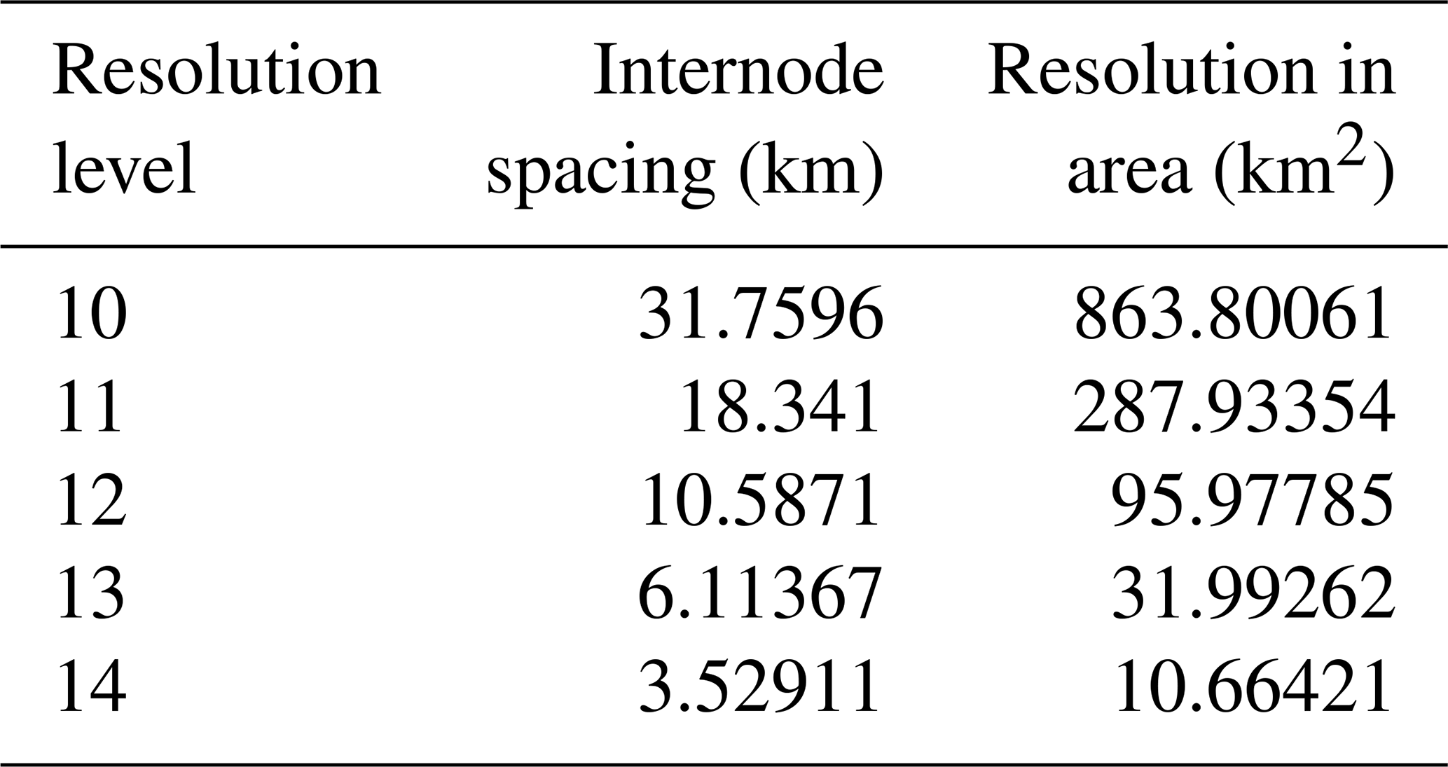
Figure 2 illustrates the simplified HydroSHEDS river networks in the Amazon basin.

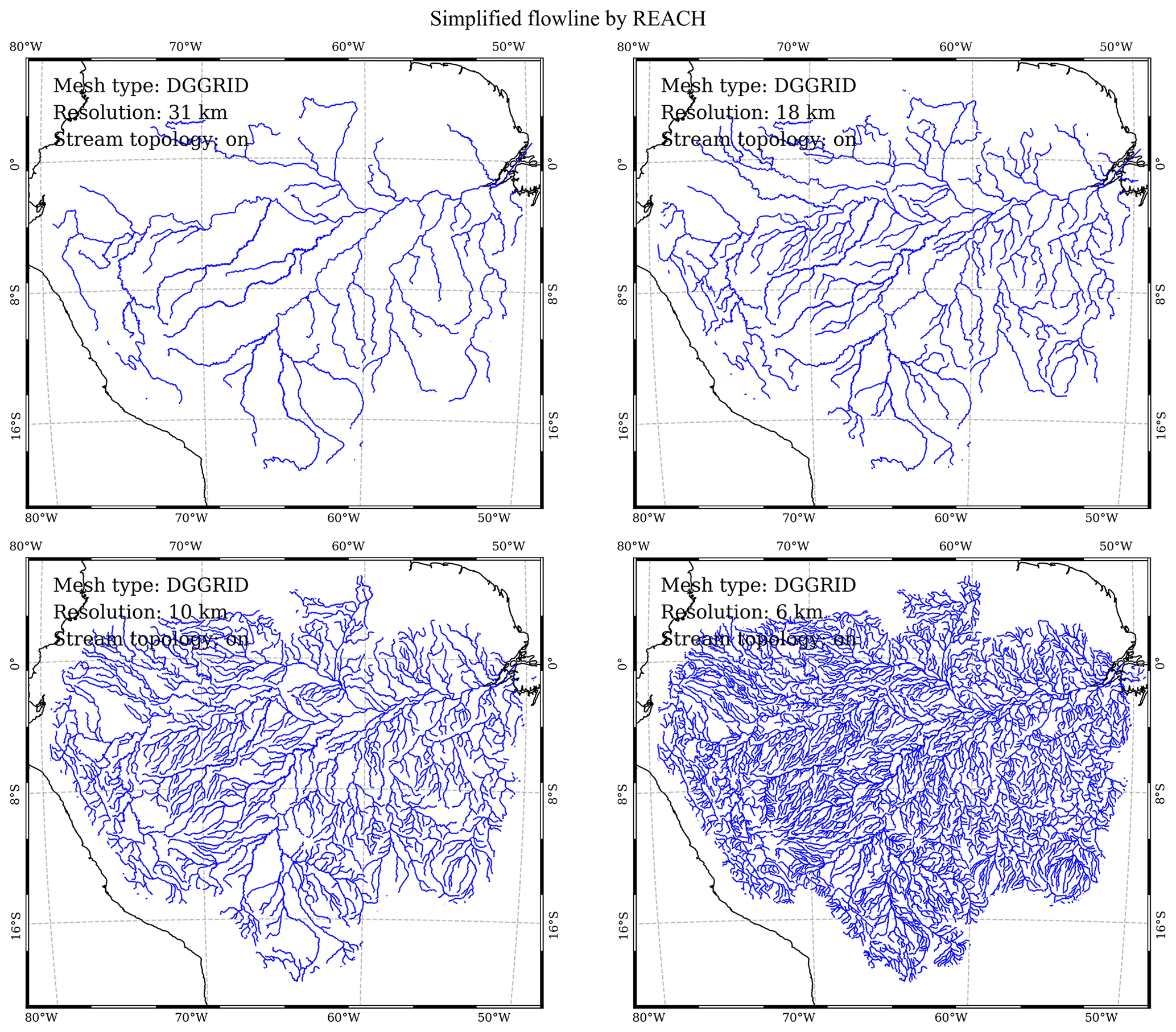
Figure 2 Simplified river networks using the REACH library at DGGRID ISEA3H level-10 to level-13 resolutions in the Amazon basin (Table 1). The black and blue lines are coastlines and river networks, respectively. As these datasets are extracted using the Amazon watershed boundary from the global HydroSHEDS river networks, there may be isolated river segments near the boundary of the basin, which are automatically excluded in the HexWatershed model.

2.2.2 Mesh generation using DGGRID

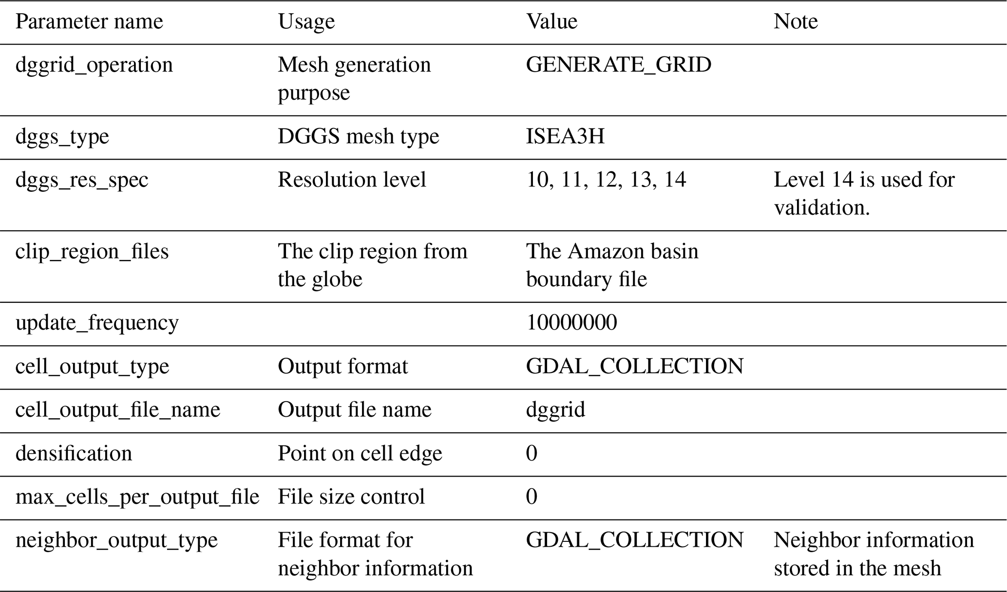
DGGRID is an actively maintained open-source library initially developed by Kevin Sahr in 2003, mainly used for generating and manipulating DGGS with diverse configurations (Sahr, 2024). The DGGRID library provides various grid geometry options, including triangles, diamonds, and hexagons. It also allows for specification of multiple refinement ratios between successive resolutions, customized orientation relative to Earth's surface, and different projection methods when generating grids such as the ISEA and FULLER projections (Sahr, 2024). A list of parameters for defining the mesh generation process is summarized in Table A1. For the complete list of parameters, please refer to the DGGRID user manual (Sahr, 2024).

DGGRID version 8.3 was used in our study to generate the ISEA3H meshes with the default orientation. A total of five resolution levels from 10 to 14 are defined (Table 1). The level-14 mesh was used for validation only.

The four spatial resolutions (levels 10–13) were selected because most large-scale hydrological models and Earth system models run at approximately 0.5° (∼ 50 km at the Equator) spatial resolution, which is similar to resolution (in length) level 10, while many large-scale hydrological models run at spatial resolutions of ∼ 5 km, similar to resolution (in length) level 13. These four spatial resolutions, therefore, cover a wide range of hydrological model applications.

Once the DGGRID model is built from its C/C$++$ source code, it can be called through several application programming interfaces (APIs), which have been implemented within the HexWatershed model (Liao, 2022a). As a result, Step 2 can be run as part of Step 3.

2.2.3 Flow direction modeling using HexWatershed

HexWatershed is a mesh-independent flow direction model for hydrological models. Unlike most flow direction models that only support structured rectangle meshes, HexWatershed supports both structured and unstructured meshes. HexWatershed includes the state-of-the-science topological relationship-based river network representation and depression removal methods to generate high-quality flow routing datasets across scales (Liao and Cooper, 2023; Liao, 2022a). These methods allow embedding of river networks and other hydrological features within the flow routing map from regional to global scales. To achieve this, HexWatershed uses a two-step approach to modeling flow direction. First, it uses the mesh–river network intersection to build the topological relationship between mesh cells and river channels (e.g., upstream–downstream channel cells). Next, it uses a hybrid stream-burning–depression-filling algorithm to generate the flow direction between all of the mesh cells. This step will first define the elevation and flow direction of the river channels and then process the remaining mesh cells. Additional explanations for these techniques are provided in the Supplement and can be found in our two-part series of studies (Liao et al., 2023a, b).

The computational geometry algorithms within HexWatershed accept all types of mesh cells (e.g., rectangle, hexagon, or triangle), and the depression removal algorithms automatically consider different numbers of neighbors when defining flow directions. Therefore, HexWatershed is mesh-independent and supports both structured and unstructured meshes.

In this study, we extended HexWatershed to support the DGGRID mesh type. Specifically, we implemented several APIs to set up a DGGRID model run and convert the DGGRID outputs to the HexWatershed model data structure (Step 2). Then we ran HexWatershed v3.0 to generate flow routing datasets using the DGGRID-generated ISEA3H meshes at four different spatial resolutions (Table 1). For each spatial resolution, the HexWatershed model simulation includes the following steps:

1. Prepare all the input datasets (outputs from Step 1) and binaries (DGGRID and HexWatershed C$++$ binaries) in a workspace folder.

2. Call the PyFlowline Python package (Liao et al., 2023a; Liao and Cooper, 2023) to generate the conceptual river networks (Fig. 1). PyFlowline is a core component in the HexWatershed model. This step includes three substeps:

   • Preprocess the vector river network datasets, i.e., simplified HydroSHEDS river networks from Step 1. This step processes the river networks further, including rebuilding the stream segment indices and (Strahler) orders.

   • Generate the DGGRID configuration file and run the DGGRID model to generate the DGGS mesh file. This is also the Step 2 in Fig. 1.

   • Model the conceptual river networks using the topological relationship-based reconstruction method.

3. Assign elevation to the mesh cells based on the raster DEM and each mesh cell boundary (Liao et al., 2022). A zonal mean resampling method is used by default.

4. Conduct the depression removal. This step includes two substeps (Liao et al., 2023b):

   • Run the topological relationship-based stream-burning on the river cells and their riparian zone cells using outputs from Steps 3b and 3c.

   • Run the revised priority-flood depression-filling for the remaining mesh cells.

5. Export and visualize the model outputs, including the flow direction map and other flow routing parameters (Liao, 2022b).

Lastly, spatial visualizations were produced using Python packages, including the Geospatial Data Abstraction Library (GDAL) (GDAL/OGR contributors, 2019) and PyEarth (Liao, 2022b).

3 Data record

These datasets contain four collections of flow routing datasets corresponding to four spatial resolutions for both the Amazon and Yukon basins (Liao, 2023). Within each collection, several files are provided, with a .readme file explaining each file. The results from resolution level 10 are used here for illustration purposes. The Supplement provides visualizations of all four dataset collections with zoom-in views. All the spatial datasets are provided using GIS file formats (e.g., GEOJSON) with the WGS84 EPSG:4326 spatial reference.

3.1 Surface elevation

The variable_polygon.geojson file is a polygon-based GEOJSON data file. The “elevation” attribute stores the modeled mean surface elevation for each DGGRID mesh cell after the depression removal (Figs. 3 and 4).

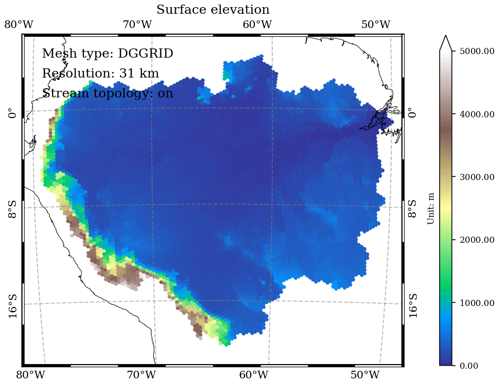
Figure 3 Spatial distribution of modeled surface elevation at DGGRID ISEA3H level-10 resolution in the Amazon basin (m).

Figure 4 Spatial distribution of modeled surface elevation at DGGRID ISEA3H level-10 resolution in the Yukon basin (m).

3.2 Surface slope

In the variable_polygon.geojson data file, the “slope” attribute stores the modeled between-cell surface slope based on the depression-free elevation difference and cell center–cell center (great-circle) distance (Figs. 5 and 6).

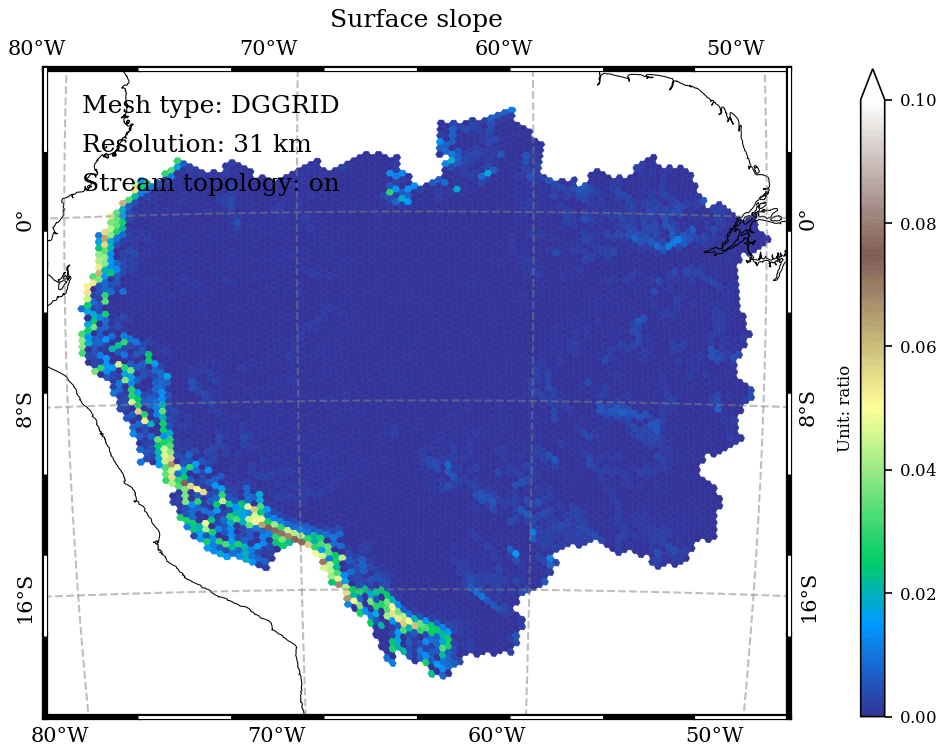
Figure 5 Spatial distribution of the modeled mesh cell center–cell center slope at DGGRID ISEA3H level-10 resolution in the Amazon basin (ratio).

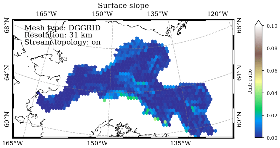
Figure 6 Spatial distribution of the modeled mesh cell center–cell center slope at DGGRID ISEA3H level-10 resolution in the Yukon basin (ratio).

3.3 Flow direction

The flow_direction.geojson file is a polyline-based GEOJSON data file. Each polyline feature defines the single flow direction (the steepest slope) from one DGGRID mesh cell center to its downslope–downstream mesh cell center (Figs. 7 and 8).

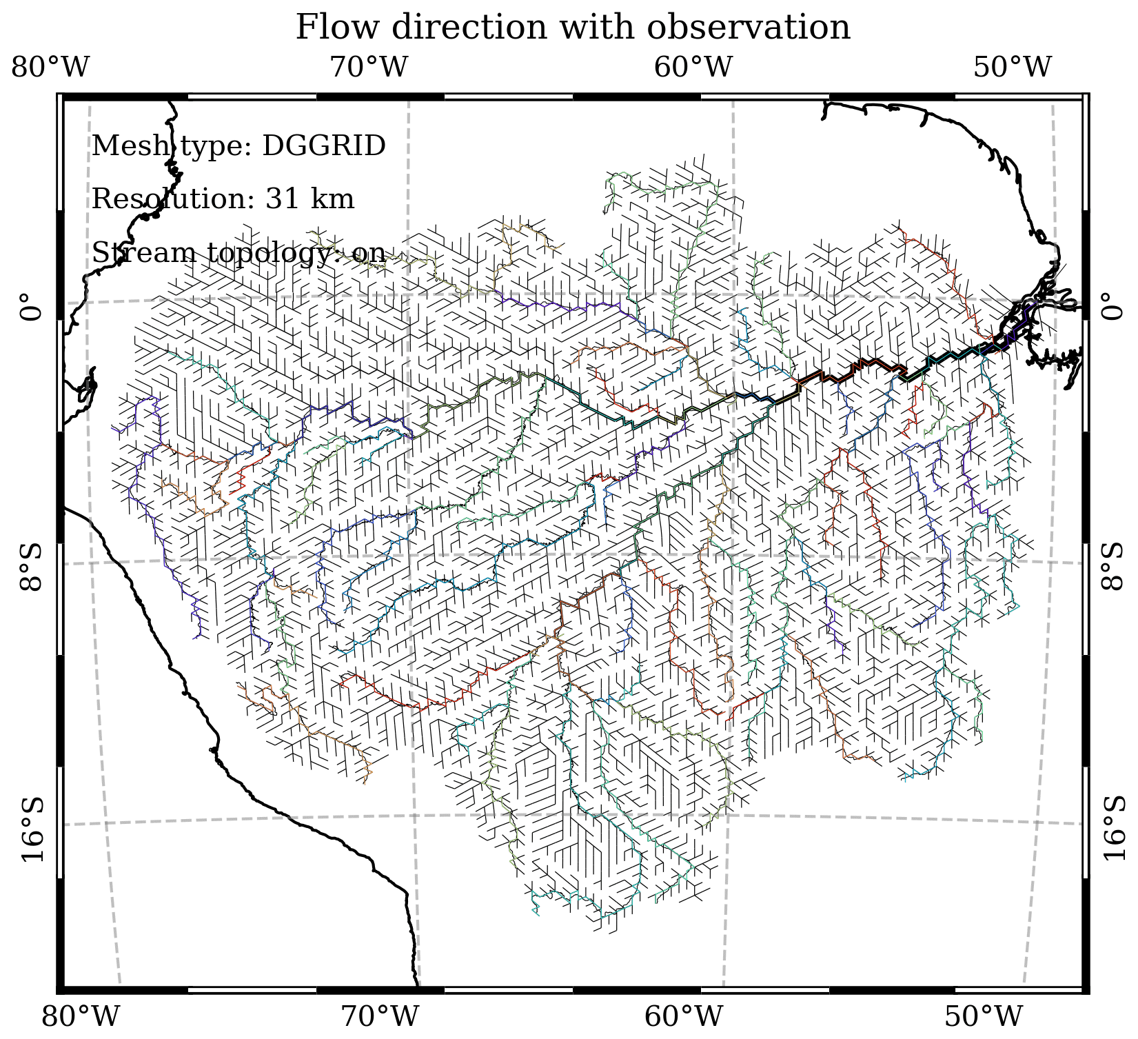
Figure 7 Modeled flow direction at DGGRID ISEA3H level-10 resolution in the Amazon basin. The black straight lines are the cell-to-cell conceptual flow direction. The line thickness is scaled with the drainage area. Colored and curved black lines are conceptual (by PyFlowline) and simplified (by REACH) HydroSHEDS river networks.

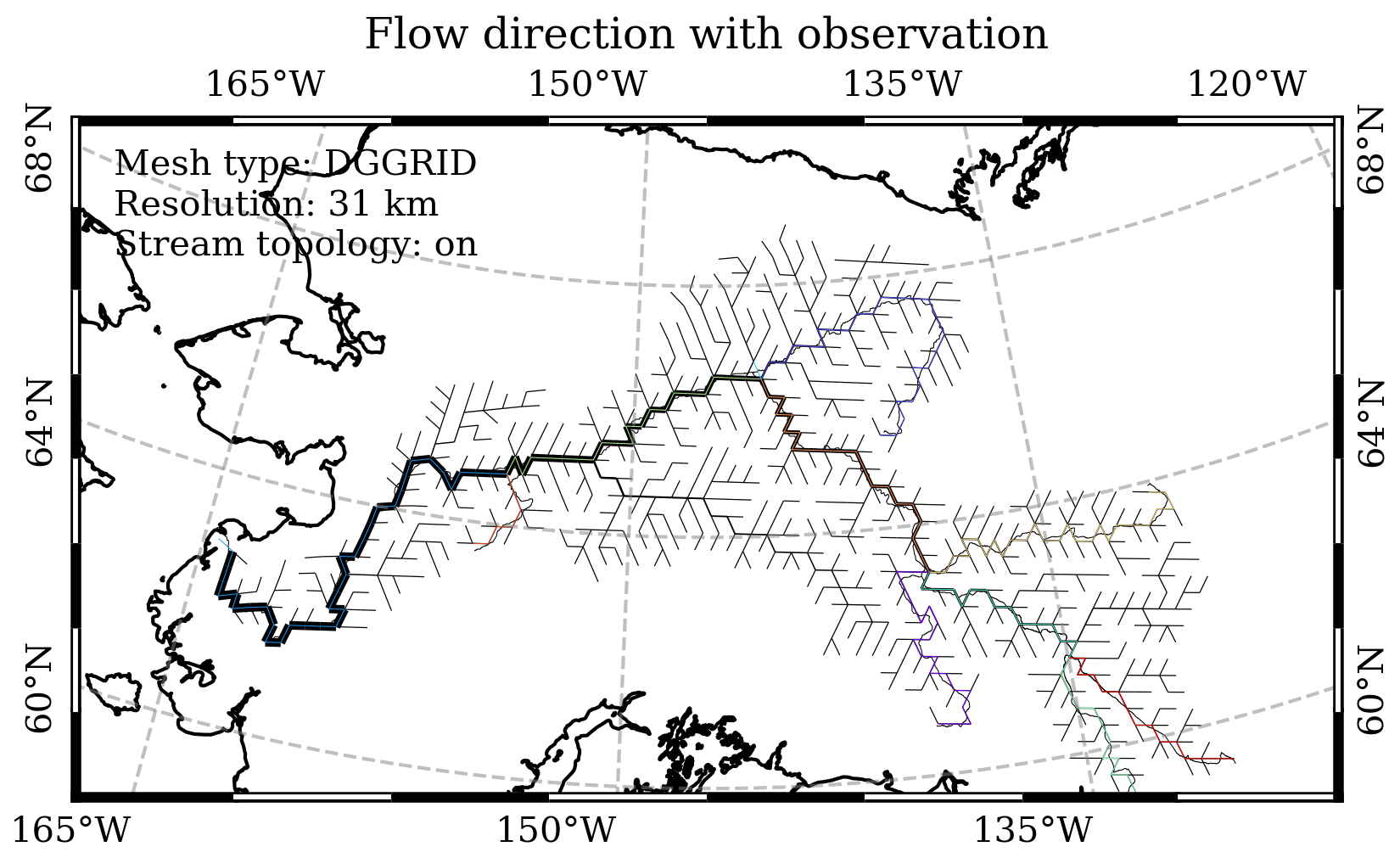
Figure 8 Modeled flow direction at DGGRID ISEA3H level-10 resolution in the Yukon basin. The black straight lines are the cell–cell conceptual flow direction. The line thickness is scaled with the drainage area. The colored and curved black lines are conceptual and simplified HydroSHEDS river networks.

3.4 Drainage area

In the variable_polygon.geojson data file, the “drainage” attribute stores the modeled total upstream drainage (spherical) area of each mesh cell (including its own area) (Figs. 9 and 10).

Figure 9 Modeled drainage area at DGGRID ISEA3H level-10 resolution in the Amazon basin (m²).

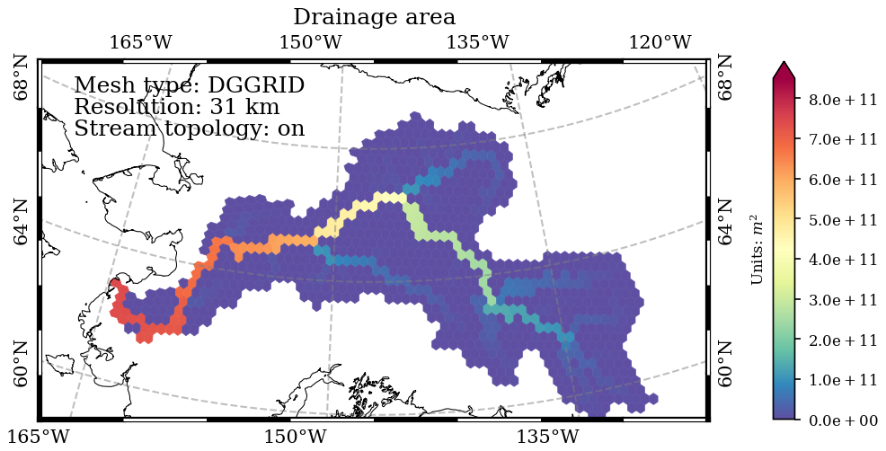
Figure 10 Modeled drainage area at DGGRID ISEA3H level-10 resolution in the Yukon basin (m²).

3.5 Travel distance

In the variable_polygon.geojson data file, the “travel_distance” attribute stores the modeled (great-circle) travel distance from each mesh cell to the basin outlets (Figs. 11 and 12). This term is also often referred to as the downstream flow length.

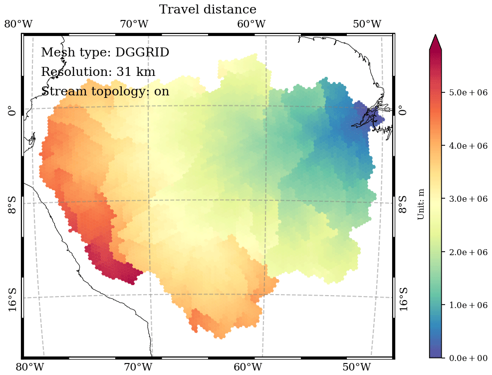
Figure 11 Modeled travel distance to the basin outlet at the DGGRID ISEA3H level-10 resolution in the Amazon basin (m).

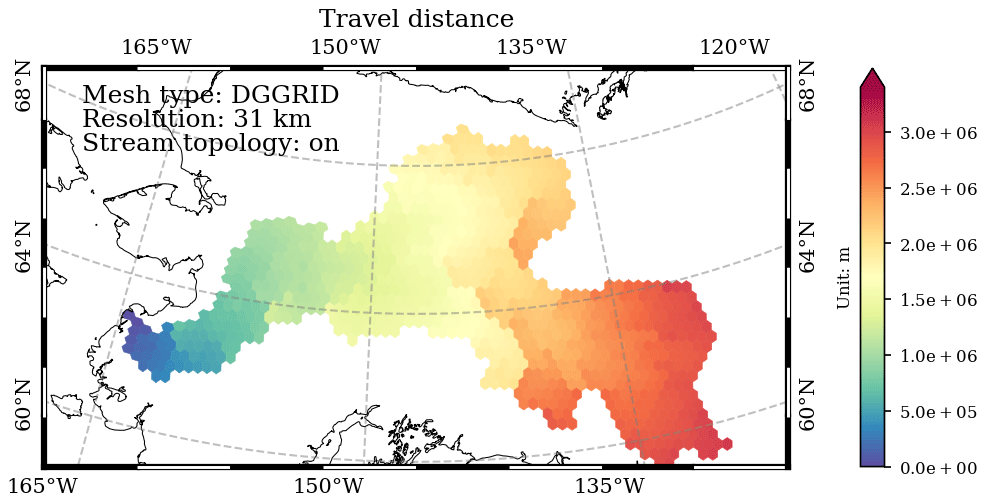
Figure 12 Modeled travel distance to the basin outlet at the DGGRID ISEA3H level-10 resolution in the Yukon basin (m).

4 Technical validation

Because the fundamental mesh structures differ from most existing datasets, we mainly rely on spatial patterns and geostatistics to evaluate our datasets. Different strategies are used for different data records. We primarily evaluate our datasets using existing flow routing datasets, i.e., HydroSHEDS products and the LBA-ECO CD-06 Amazon River Basin Land and Stream Drainage Direction and DEM datasets (Mayorga et al., 2012; Saatchi, 2013).

4.1 River networks

The river networks are the core intermediate results generated by the HexWatershed model in our workflow (Fig. 1). Although these datasets do not cover the entire study domain, they illustrate how closely the modeled river networks match the REACH-generated river networks (Fig. 2). In this study, we employed the “area of difference” method to assess their accuracy (Liao et al., 2022, 2023a) (Fig. D1 in Sect. D1). This method uses the area to represent discrepancies in line features, such as river networks. When two or more line features intersect, the intersected segments can create enclosed polygons. We then calculate and compare the areas of these polygons to quantify the differences formed by flowline intersections. Figures 13 and 14 illustrate the evaluation of river networks using this method in the Amazon and Yukon basins, respectively.

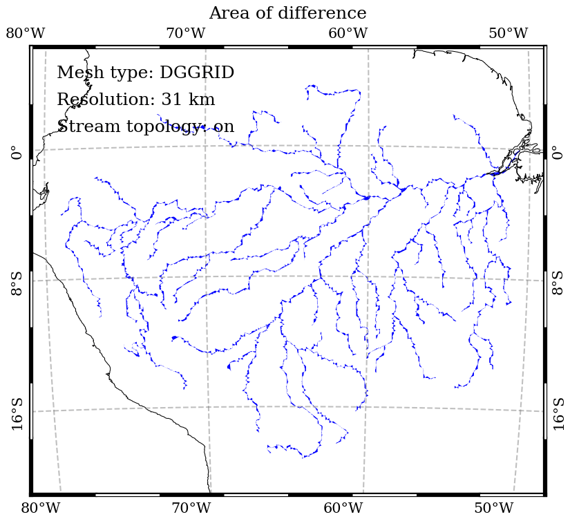
Figure 13 Validation of modeled river networks against HydroSHEDS river networks (REACH simplified) using the area of difference at DGGRID ISEA3H level-10 resolution in the Amazon basin. The total area of difference is 4.5×10⁵ km².

Figure 14 Validation of modeled river networks against HydroSHEDS river networks (REACH simplified) using the area of difference at DGGRID ISEA3H level-10 resolution in the Yukon basin. The total area of difference is 6.0×10⁴ km².

4.2 Surface elevation

We employed a sphere-resampling method to assess the surface elevation data through the following steps: (1) utilizing the DGGRID ISEA3H level-14 mesh (the highest resolution in the current workflow) as the sampling pool, (2) randomly selecting N cells as points of interest and recording their center locations, and (3) extracting elevation values from the data records and existing DEM datasets based on the chosen N longitude–latitude pairs. A scatterplot featuring N=500 sampling points demonstrates that the modeled elevations closely match those of the existing high-resolution raster DEMs (Fig. 15).

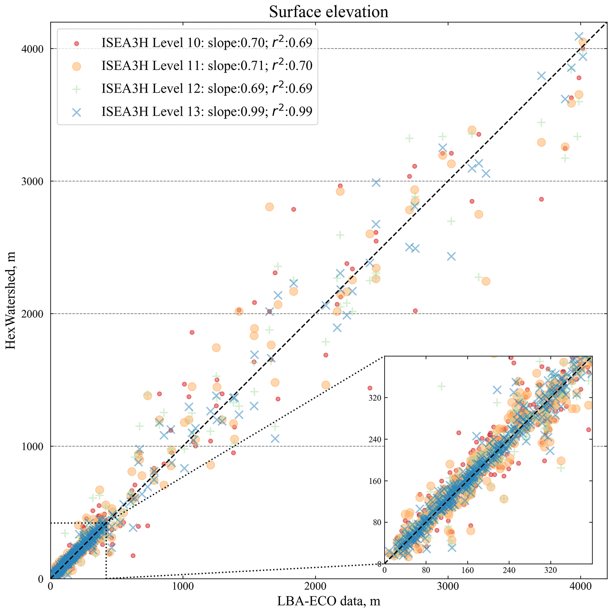
Figure 15 Validation of the modeled surface elevation in the Amazon basin from four DGGRID mesh resolutions. The x axis is the sampled elevation from the LBA-ECO DEM datasets. The y axis is the sampled surface elevation from our records (m). The mini-plot is a zoom-in view of the lower left.

The modeled surface elevation in the Yukon basin is slightly worse than that in the Amazon basin (Fig. 16). One reason is that the spatial resolution of the LBA-ECO DEM (30 s) is twice that of the HydroSHEDS DEM (15 s). Meanwhile, the Amazon basin has relatively flat terrain compared with the Yukon basin. This leads to different biases during the zonal mean resampling procedure (Liao et al., 2022).

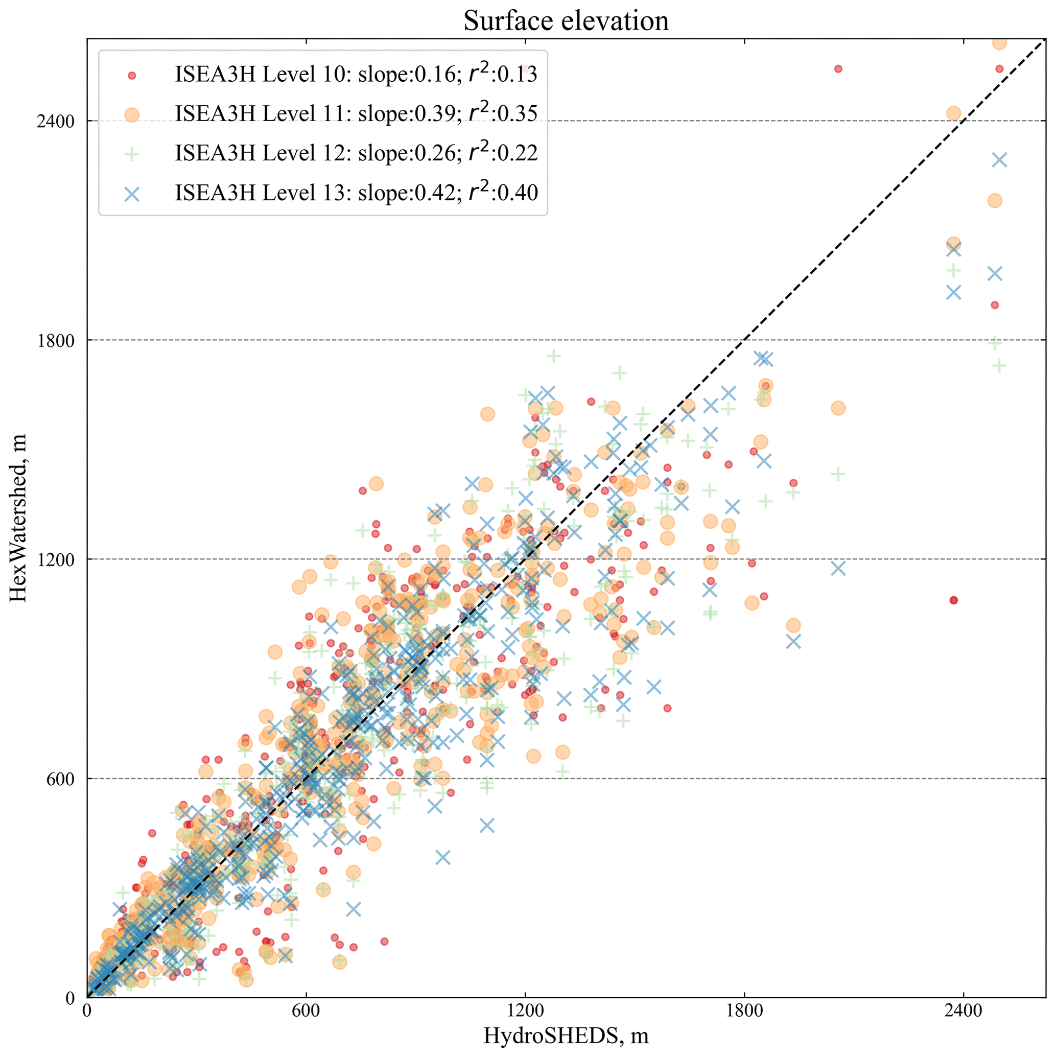
Figure 16 Validation of the modeled surface elevation in the Yukon basin from four DGGRID mesh resolutions. The x axis is the sampled elevation from the HydroSHEDS DEM datasets. The y axis is the sampled surface elevation from our records (m).

4.3 Flow direction

Given that flow direction is a vector field, a direct comparison between the modeled flow directions and the existing D4-based or D8-based flow direction datasets is not feasible. Instead, we conducted a visual examination of the modeled flow directions using the simplified HydroSHEDS river networks. As depicted in Figs. 7 and 8, the modeled flow directions consistently align with the simplified HydroSHEDS river networks across all four resolutions, consistent with our previous study (Liao et al., 2023b). Additionally, flow directions can be validated indirectly using the drainage area since they are closely interconnected.

4.4 Drainage area

The sphere resampling method (Sect. 4.2) could not be directly applied to the drainage area due to issues related to resolution mismatch and spatial dependence. As an alternative, we conducted a comparative analysis using major tributaries along the Amazon River and Yukon River, including their river mouths.

In the Amazon basin, we selected seven tributary outlets, and their locations are provided in the Supplement. The scatterplot shows that the modeled drainage areas are consistent with the existing LBA-ECO drainage datasets (Fig. 17).

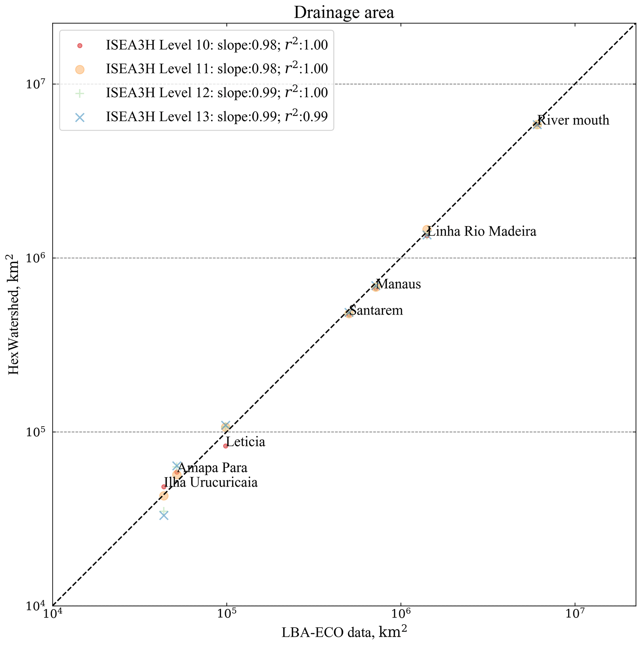
Figure 17 Validation of the modeled drainage area of seven tributaries (including the river mouth) along the Amazon River from four DGGRID mesh resolutions. The x axis is the drainage area from the LBA-ECO CD-06 Amazon River Basin Land and Stream Drainage Direction datasets (converted from flow accumulation). The y axis is the modeled drainage area (km²). Both the x and y axes are on the log scale.

In the Yukon basin, we selected six tributary outlets, and their locations are provided in the Supplement. Among these tributaries, only the modeled drainage area at resolution level 10 at the Kooyukuk River is underestimated (Fig. 18).

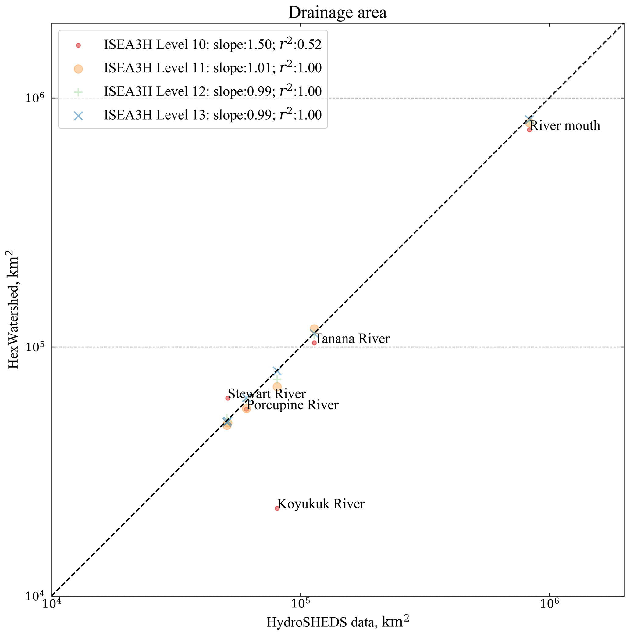
Figure 18 Validation of the modeled drainage area of six tributaries along the Yukon River from four DGGRID mesh resolutions. The x axis is the drainage area from the HydroSHEDS datasets. The y axis is the modeled drainage area (km²). Both the x and y axes are on the log scale.

4.5 Travel distance

Similar to the drainage area, we evaluated the modeled travel distance using the selected tributary outlets, excluding the river mouths. In the Amazon basin, the scatterplot shows that the modeled travel distances are consistent with the existing LBA-ECO CD-06 flow length datasets (Fig. 19). However, the modeled travel distances are slightly longer than those of the LBA-ECO datasets. This is possibly caused by the additional length added near the Amazon River delta region. A similar pattern is also observed in the Yukon basin (Fig. 20).

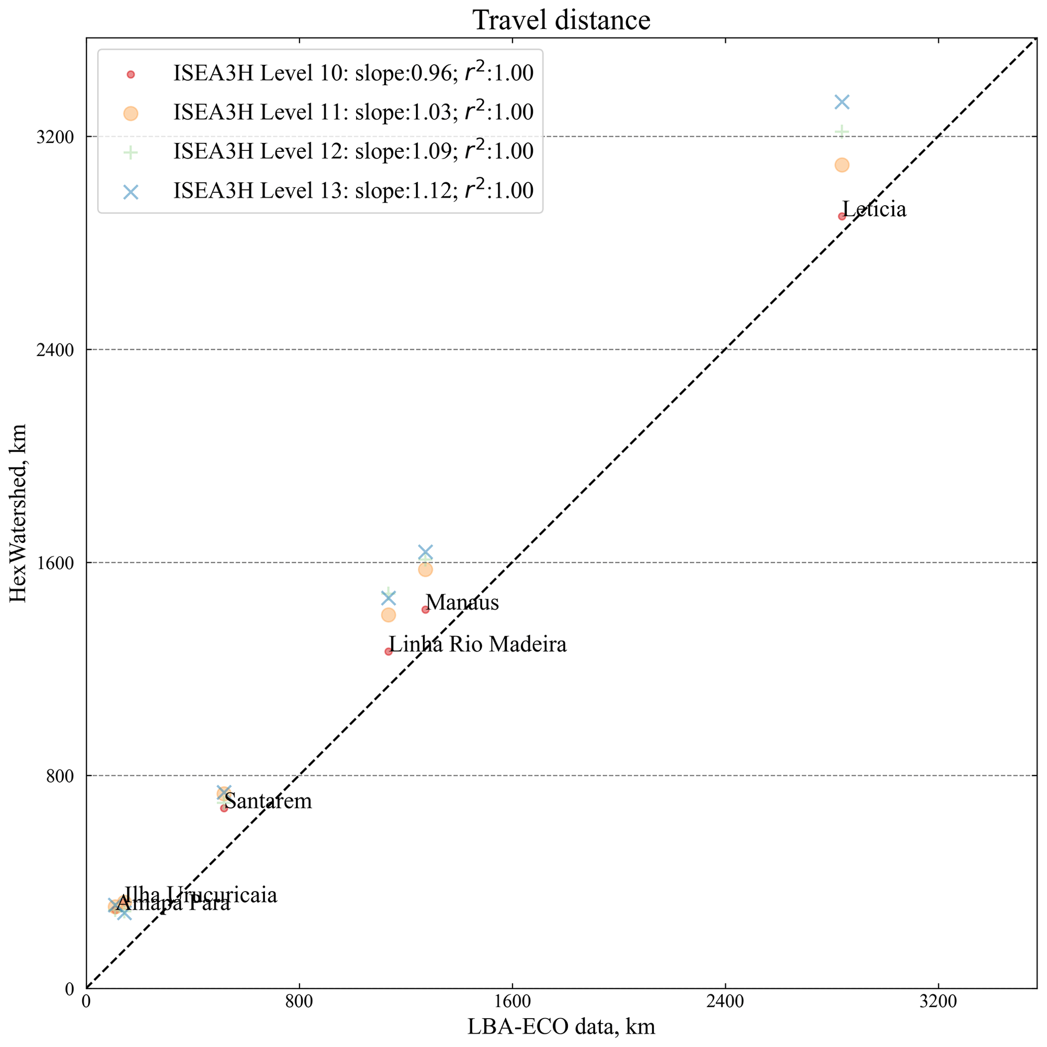
Figure 19 Validation of the modeled travel distance of six tributaries along the Amazon River from four DGGRID mesh resolutions. The x axis is the travel distance from the LBA-ECO CD-06 Amazon River Basin Land and Stream Drainage Direction datasets. The y axis is the modeled travel distance (km).

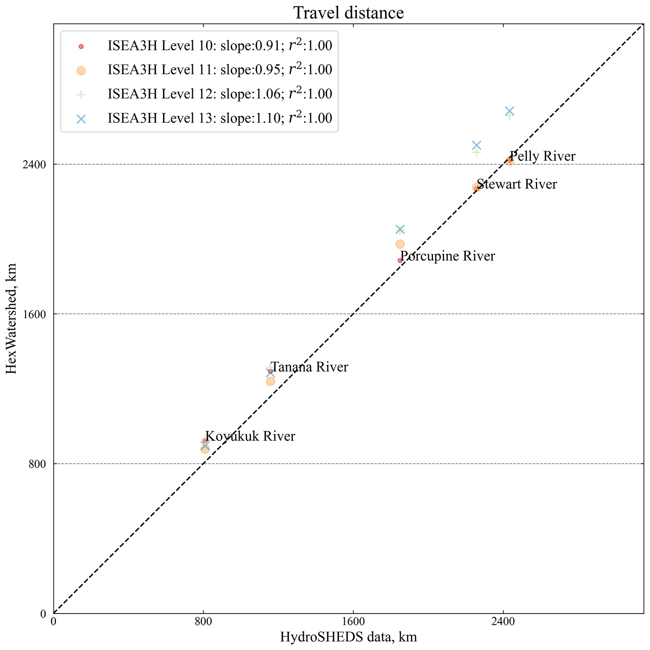
Figure 20 Validation of the modeled travel distances of six tributaries along the Yukon River from four DGGRID mesh resolutions. The x axis is the travel distance from the HydroSHEDS datasets. The y axis is the modeled travel distance (km).

5 Discussion

5.1 Limitation

Although our datasets represent an important step forward in flow routing capability, they are not without limitations. Through our practice, we have identified the following limitations and provided corresponding solutions for future improvements:

1. As a pioneering dataset, our dataset records were not produced from a unified data source, especially for the DEM component. This is because nearly all of the existing global DEM datasets use the GCS spatial reference, and the quality of the DEM gradually decreases from the Equator to the high latitudes due to the spatial distortion (Liao et al., 2020). This is also part of the reason why the modeled surface elevation in the Yukon basin is not as good as that in the Amazon basin. However, the workflow we developed is generally robust even though there are potential issues in the DEM datasets.

2. The HexWatershed model does not accommodate braided rivers currently, potentially introducing uncertainty into the flow direction, particularly near river deltas. However, since most hydrological models also lack support for braided rivers, this limitation is not considered critical.

3. The modeled drainage area and travel distance were slightly higher than observed in the Amazon basin (Fig. 19). We interpret this as being due to the inclusion of the complex delta region, which suggests that a similar bias could arise in similar deltaic regions worldwide. To address this, it is recommended to use high-resolution meshes (such as ISEA3H resolution level 13) to mitigate its impact on model performance for large-scale hydrological and Earth system models. Alternatively, explicit modeling of delta connectivity using HexWatershed can also be an effective solution.

4. Our method does not consider large lake water bodies in the workflow. Therefore, these datasets may not be suitable for hydrological applications that focus on lake routing. We plan to explicitly consider lakes, especially large lakes, in future developments.

5. Due to computational constraints and input dataset quality, we only generated flow routing datasets at four spatial resolutions in the Amazon and Yukon basins. To evaluate model performance and suitability at finer spatial resolutions (e.g., < 5 km), additional simulations are needed. Additionally, a global-scale dataset will be made available once computational efficiency has been enhanced.

5.2 Usage

The datasets are primarily stored using the JavaScript Object Notation (JSON) and GEOJSON formats. Some datasets are also provided in the GeoPackage and (Geo)Parquet file formats tailored to high-performance operations and visualizations. Most scientific programming languages, including Python, C$++$, R, and MATLAB, provide functions or public libraries to read these file formats. The datasets for these two basins are distributed with global coverage, but users can extract portions of the dataset using GIS operations. For example, users can extract subbasins for regional hydrological simulations or convert them into other common scientific file formats, including the network Common Data Form (NetCDF) or Hierarchical Data Format (HDF).

These datasets are suitable for regional and large-scale spatially distributed hydrological and river routing models, including the Model for Scale Adaptive River Transport (MOSART) (Li et al., 2013). Additionally, users can derive other flow routing parameters like the topographic wetness index (TWI) and Manning's roughness coefficient (n) from these datasets.

We also provide an online Jupyter notebook tutorial that can be used to reproduce these datasets in a browser at https://github.com/changliao1025/hexwatershed_tutorial (last access: 17 May 2024). This tutorial can be modified to generate similar datasets using other DGGRID-supported mesh types and resolutions or in different river basins.

6 Data availability

The datasets are stored in the Zenodo repository: https://doi.org/10.5281/10.5281/zenodo.8377765 (Liao, 2023).

7 Code availability

The REACH tool can be accessed from the Zenodo repository: https://doi.org/10.5281/zenodo.8368261 (Engwirda, 2023). The DGGRID model can be accessed from the GitHub repository: https://github.com/sahrk/DGGRID (last access: 23 September 2023) (Sahr, 2024). The HexWatershed model can be installed through the Conda Python platform: https://anaconda.org/conda-forge/hexwatershed (, ) (Liao, 2022a; Liao and Cooper, 2022). A tutorial of the HexWatershed is provided at: https://mybinder.org/v2/gh/changliao1025/hexwatershed_tutorial/HEAD (Liao, 2024). The source code to reproduce the datasets and figures is stored in the Zenodo repository: https://doi.org/10.5281/zenodo.14968053 (Liao, 2025).

8 Conclusions

We have produced pioneering ISEA3H DGGS-based hierarchical flow routing datasets in the Amazon basin and Yukon basin, available at four spatial resolutions (in length) (29.42, 16.99, 9.81, and 5.66 km). Extensive evaluation confirms their consistency with existing high-resolution terrain data and HydroSHEDS river networks. Because our method is mesh-independent, similar flow routing datasets can also be generated on DGGS with various configurations or even other unstructured grid meshes. Adoption of these datasets by hydrological models will enhance the performance of spatially distributed hydrological models of these two basins and similar regions worldwide.

Appendix A: Model configurations

A1 DGGRID model configurations

Table A1 List of the DGGRID mesh generation parameters used in this study.

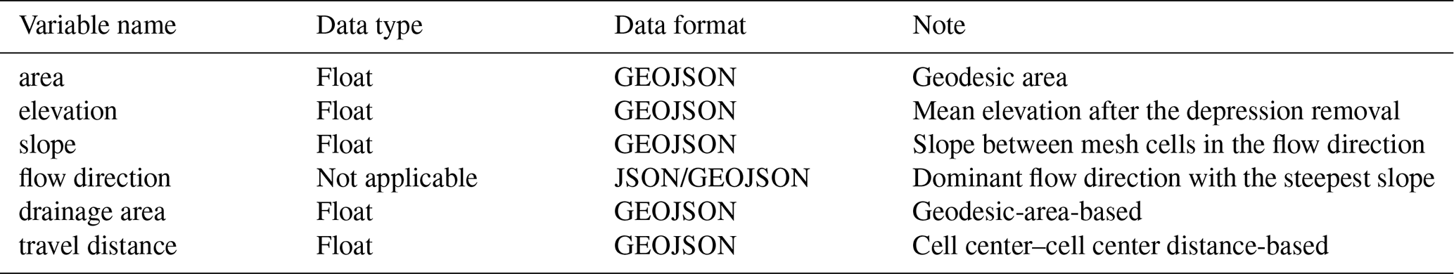
A2 HexWatershed model configurations

Table A2 List of data records produced by HexWatershed in the Amazon basin.

Appendix B: HexWatershed method description

B1 PyFlowline

The PyFlowline model is a core submodule within the HexWatershed model. PyFlowline generates the mesh-cell-based conceptual river networks using three steps: (1) flowline simplification, which removes undesired flowlines and builds the topological relationships; (2) mesh generation, which creates customized meshes based on model configuration, e.g., now supporting APIs in generating a DGGRID mesh; and (3) topological relationship reconstruction. This algorithm uses the intersection between flowlines and mesh cells to reconstruct the cell-to-cell topological relationships.

B2 HexWatershed

HexWatershed is a mesh-independent flow direction model and fully supports all the mesh types generated by PyFlowline. It defines flow direction using a two-step approach. First, it uses a hybrid breaching–filling stream-burning method to define the flow direction for river networks and their riparian zones. Second, it uses a revised priority-flood algorithm to conduct depression-filling and defines the flow direction for the remaining mesh cells. A list of the other flow routing parameters is generated through this process.

A video describing the hybrid stream-burning and depression-filling algorithm is provided using the ISEA3H level-11 simulation animation at https://www.youtube.com/watch?v=G2uTHlCUMTc (last access: 24 September 2024).

Appendix C: Full data record visualization

C1 Amazon basin

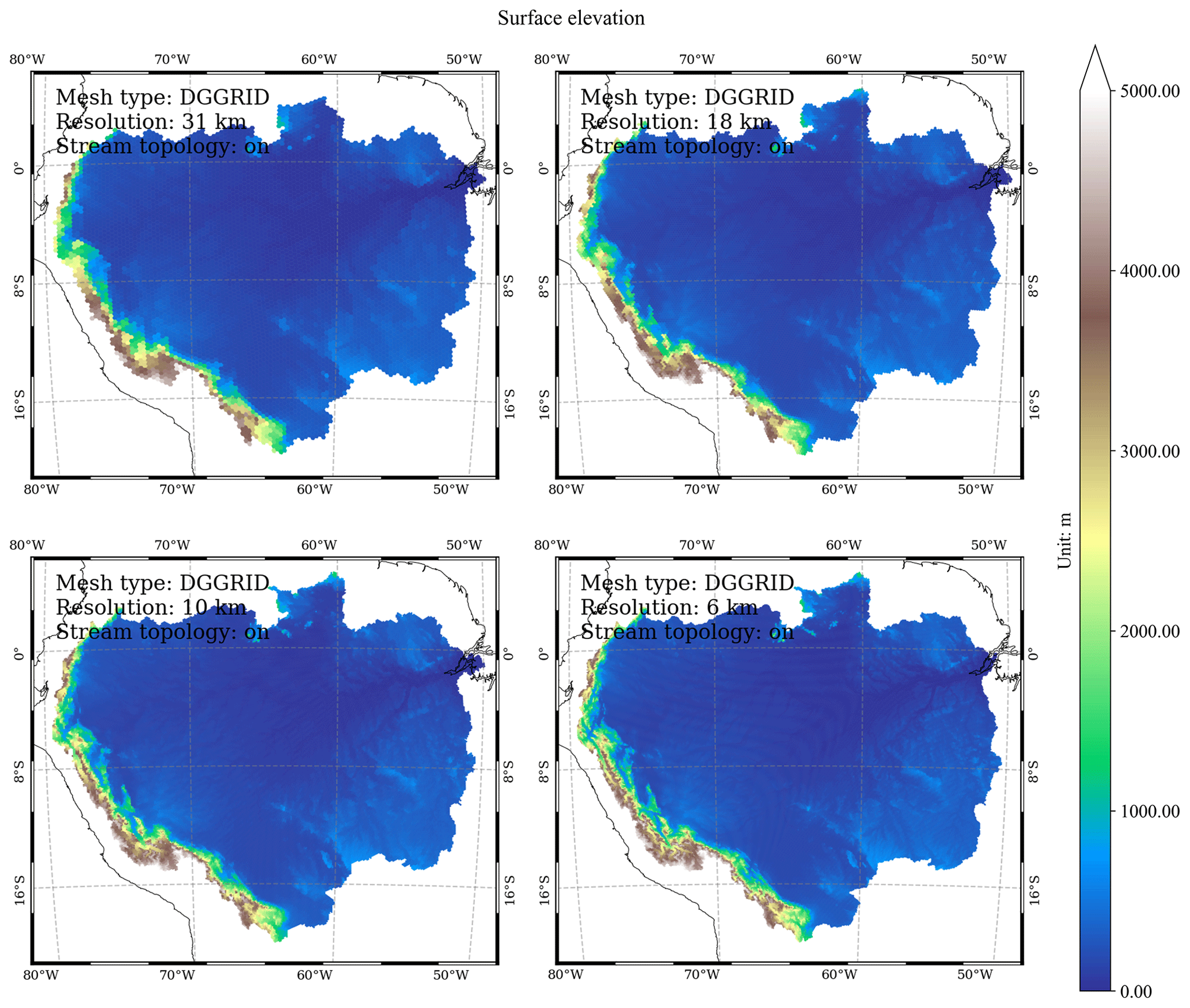
Figure C1 Spatial distribution of modeled surface elevation at the DGGRID ISEA3H level-10 to level-13 resolutions in the Amazon basin (m).

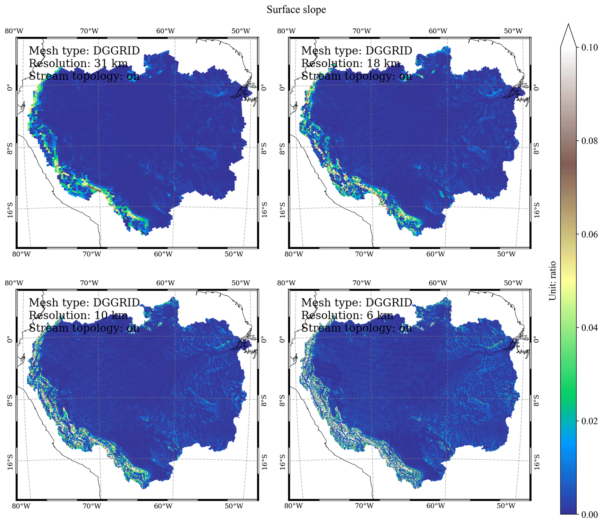
Figure C2 Spatial distribution of the modeled mesh cell center–cell center slope at DGGRID ISEA3H level-10 to level-13 resolutions in the Amazon basin (ratio).

Figure C3 Modeled flow direction at the DGGRID ISEA3H level-10 to level-13 resolutions in the Amazon basin. The black lines are the cell-to-cell flow direction. The line thickness is scaled with the drainage area. Colored and detailed black lines are conceptual and simplified HydroSHEDS river networks.

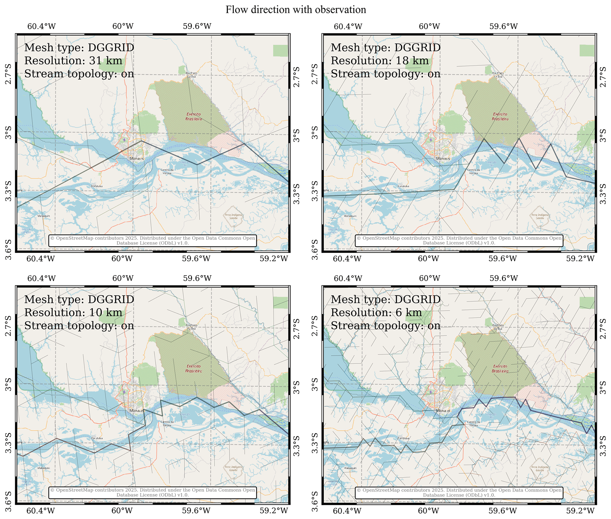
Figure C4 Zoom-in views of the modeled flow direction at the DGGRID ISEA3H level-10 to level-13 resolutions in the Amazon basin near Manaus. The black lines are the cell-to-cell flow direction. The line thickness is scaled with the drainage area. The colored and detailed black lines are conceptual and simplified HydroSHEDS river networks. The base images are from ©OpenStreetMap contributors 2024, distributed under the Open Data Commons Open Database License (ODbL) v1.0.

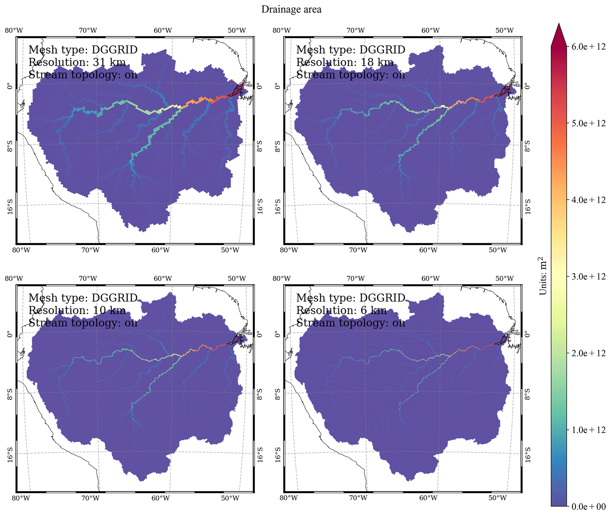
Figure C5 Modeled drainage area at the DGGRID ISEA3H level-10 to level-13 resolutions in the Amazon basin (m²).

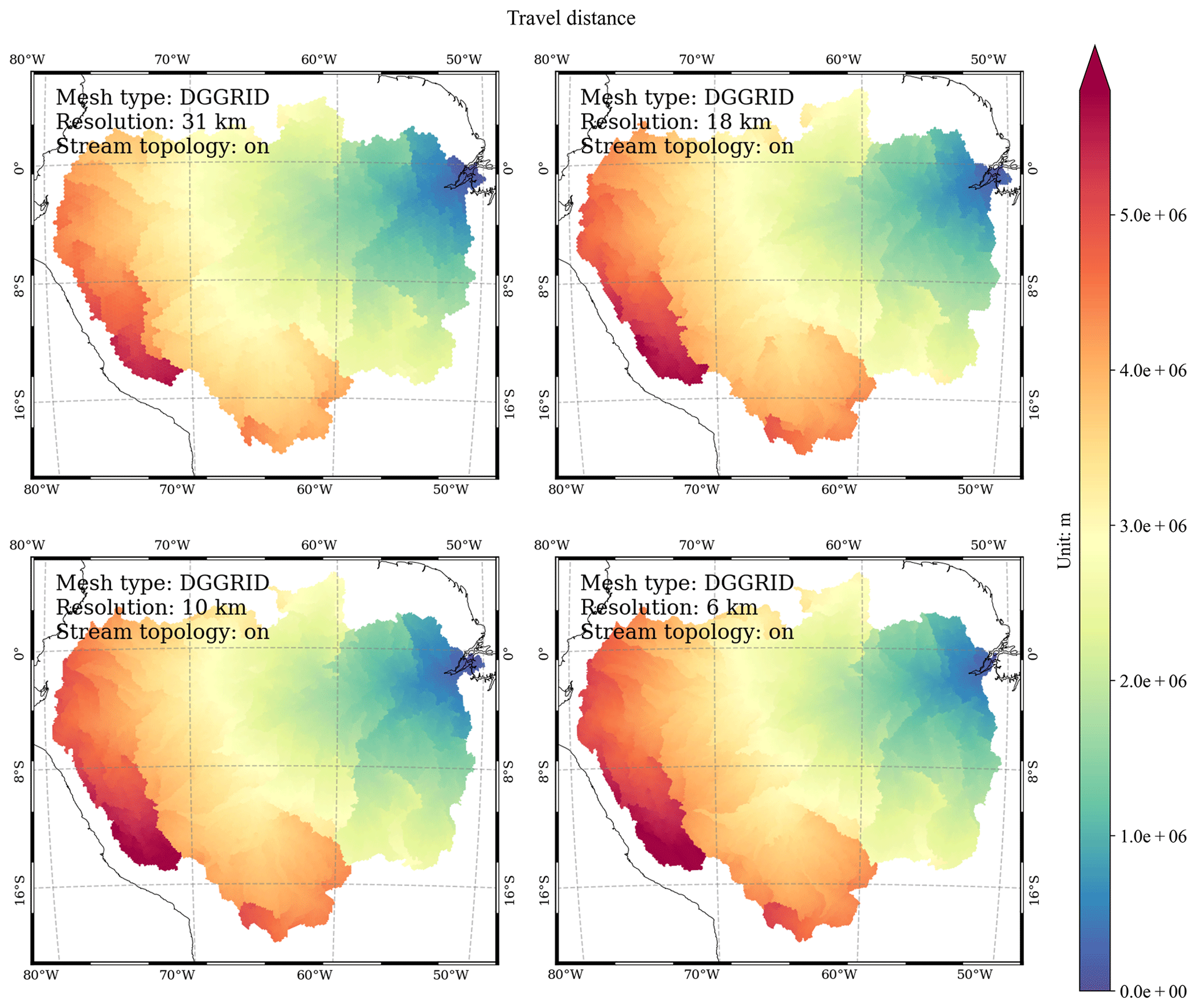
Figure C6 Modeled travel distance to the basin outlet at DGGRID ISEA3H level-10 to level-13 resolutions in the Amazon basin (m).

C2 Yukon basin

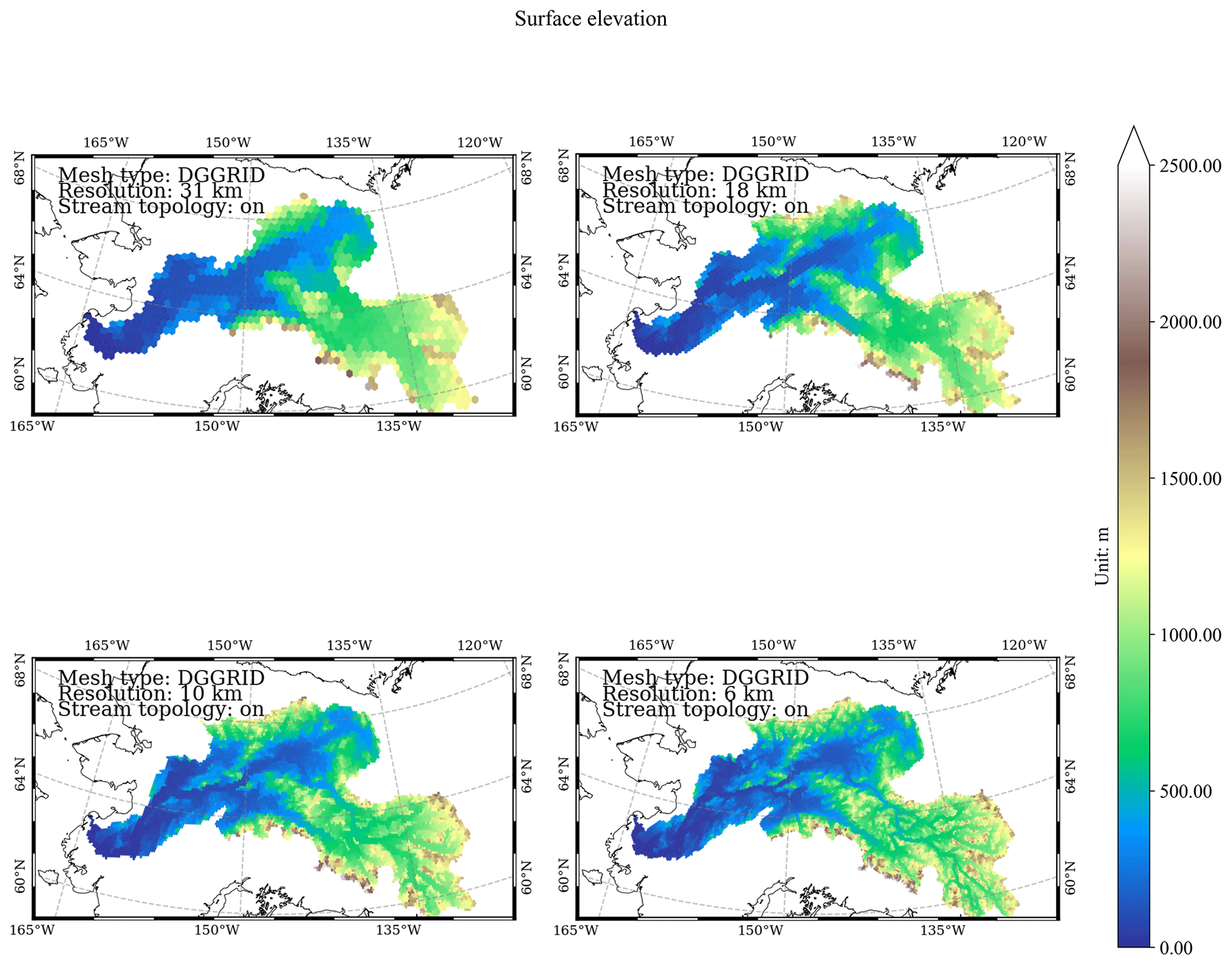
Figure C7 Spatial distribution of modeled surface elevation at the DGGRID ISEA3H level-10 to level-13 resolutions in the Yukon basin (m).

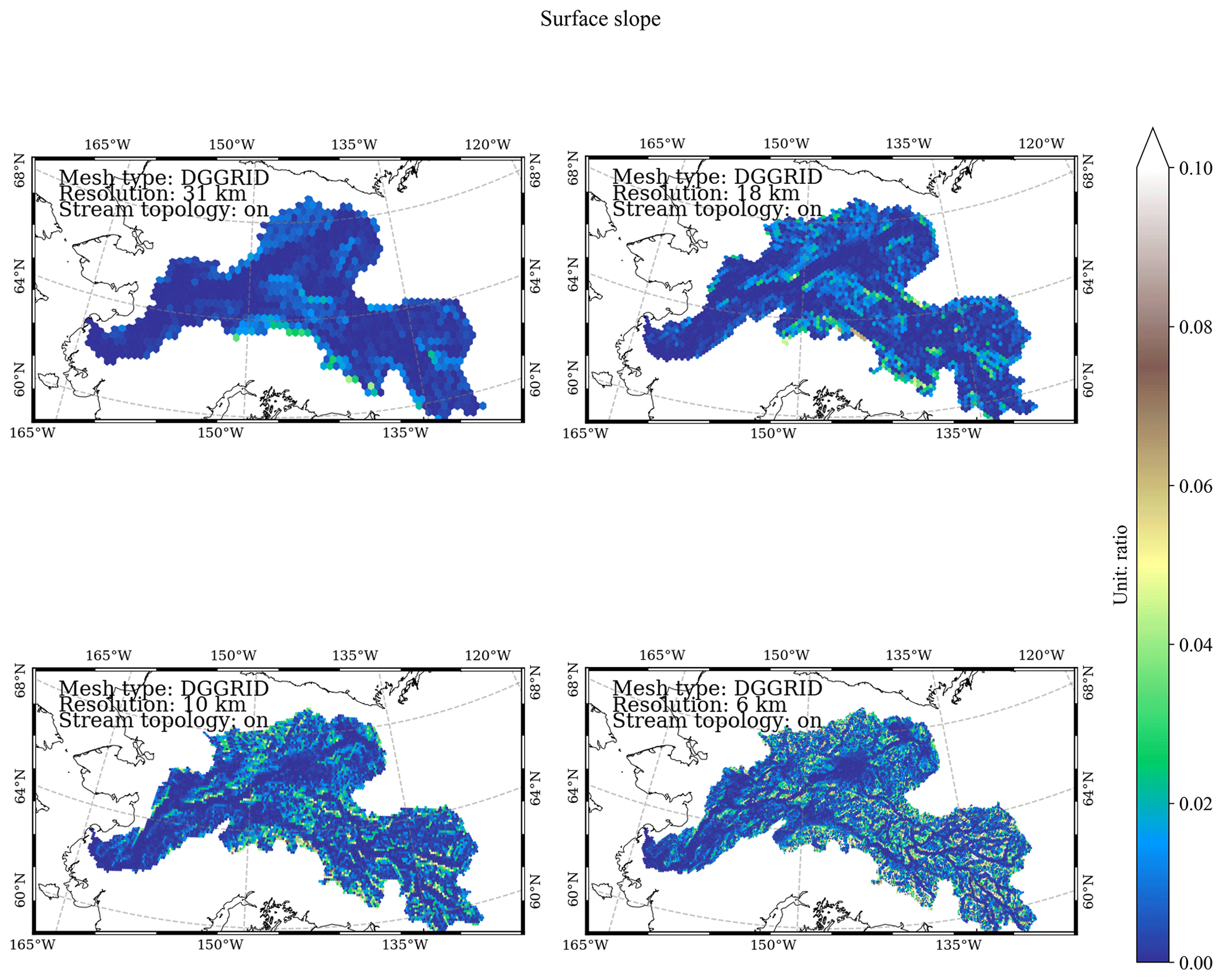
Figure C8 Spatial distribution of the modeled mesh cell center–cell center slope at DGGRID ISEA3H level-10 to level-13 resolutions in the Yukon basin (ratio).

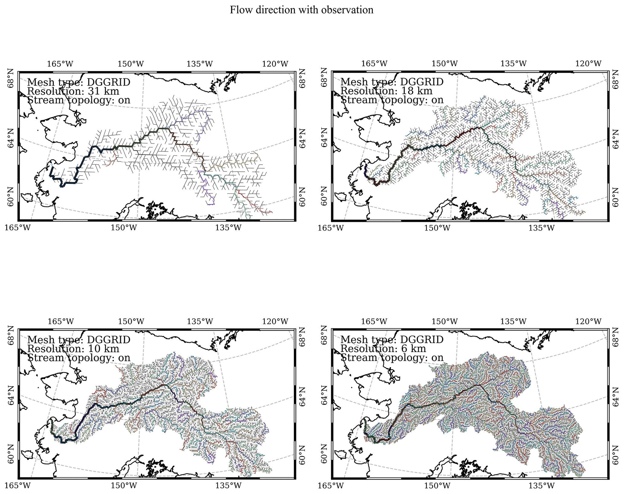
Figure C9 Modeled flow direction at DGGRID ISEA3H level-10 to level-13 resolutions in the Yukon basin. Black lines are the cell-to-cell flow direction. Line thickness is scaled with drainage area. Colored and detailed black lines are conceptual and simplified HydroSHEDS river networks.

Figure C10 Modeled drainage area at the DGGRID ISEA3H level-10 to level-13 resolutions in the Yukon basin (m²).

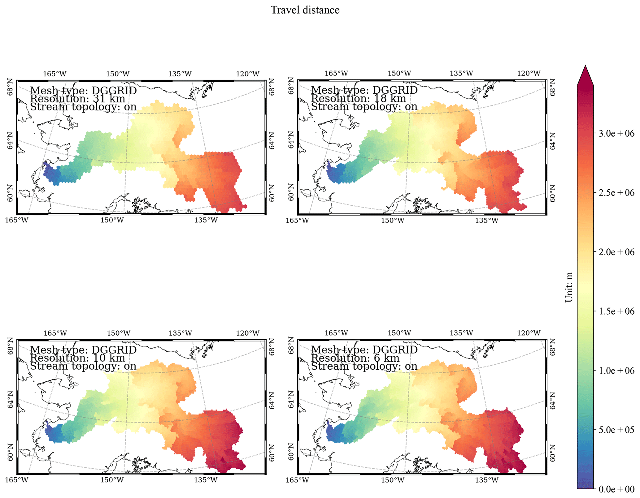
Figure C11 Modeled travel distance to the basin outlet at the DGGRID ISEA3H level-10 to level-13 resolutions in the Yukon basin (m).

Appendix D: Data validation

D1 Area-of-difference method

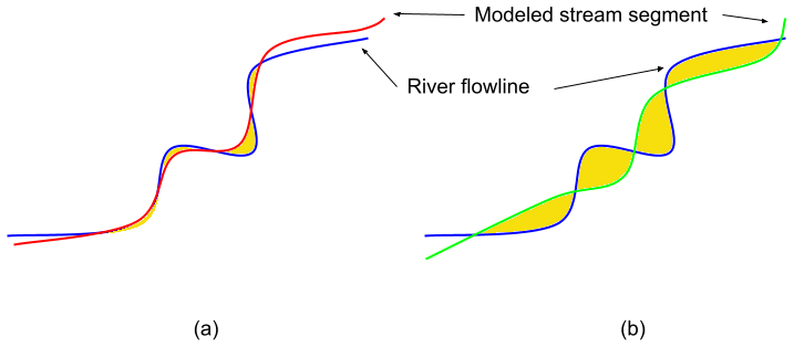
Figure D1 Illustration of the area of differences based on line feature intersections. Blue line features are actual river flowlines. Red and green line features are modeled flowlines from different simulations. Yellow-filled polygons are the product of line intersections from actual and modeled flowlines. The smaller the total area of these polygons is, the closer the modeled flowline is to the actual flowline. As a result, the modeled flowline in panel (a) is closer to or better than that in panel (b).

The area of differences can be calculated using Python scripting in the following steps:

1. Convert modeled conceptual flowlines into edge-based flowlines A.

2. Intersect the edge-based flowlines A with the simplified flowlines B to obtain all the vertices in list C.

3. Classify the vertices C into different types of vertices (i.e., shared by the number of flowlines).

4. Split both A and B using C to obtain a list of flowlines D.

5. Build all the polygons enclosed by connected flowlines in D using a cycling algorithm and calculate their areas.

6. Sum up the areas to obtain the total area of difference.

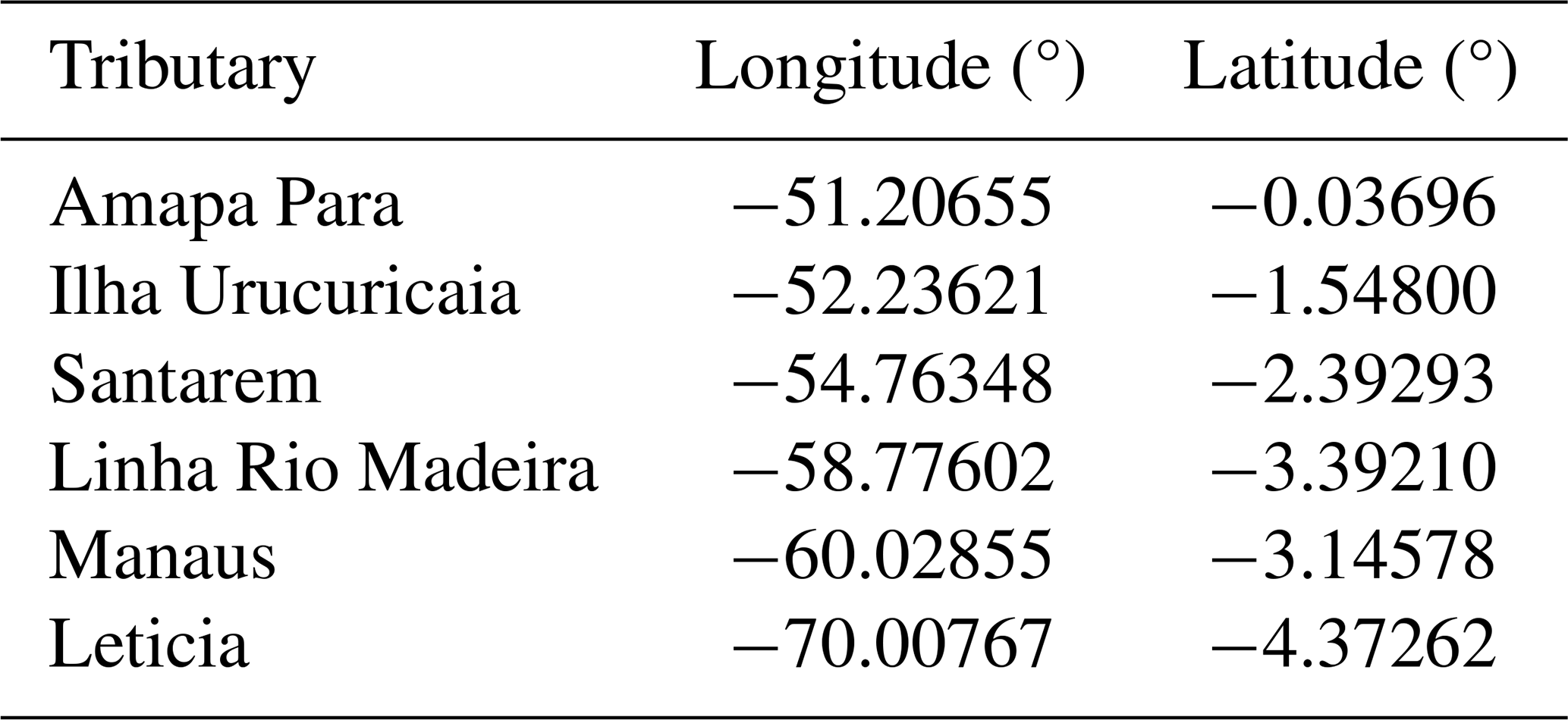
D2 Tributaries along the Amazon River

Table D1 List of tributary outlets along the Amazon River used for drainage area and travel distance validations.

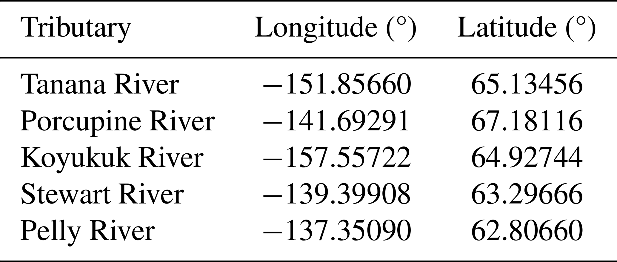
D3 Tributaries along the Yukon River

Table D2 List of tributary outlets along the Yukon River used for drainage area and travel distance validations.