Satellite-derived global-ocean phytoplankton phenology indices

Phytoplankton bloom phenology is an important indicator for the monitoring and management of marine resources and the assessment of climate change impacts on ocean ecosystems. Despite its relevance, there is no long-term and sustained observational phytoplankton phenological product available for global-ocean implementation. This need is addressed here by providing a phenological data product (including among other seasonal metrics, the bloom initiation, termination, duration, and amplitude timing) using satellite-derived chlorophyll-a data from the Ocean Colour Climate Change Initiative. This multi-decadal data product provides the phenology output from three widely used bloom detection methods at three different spatial resolutions (4, 9, and 25 km), allowing for both regional- and global-scale applications. When compared to each other on global scales, there is general agreement between the detection methods and between the different resolutions. Regional differences are evident in coastal domains (particularly for different resolutions) and in regions with strong physical–biogeochemical transitions (notably for different detection methods). This product can be used towards the development of national and global biodiversity assessments, for pelagic ecosystem mapping, and for monitoring change in climate sensitive regions relevant for ecosystem services. The data set is published in the Zenodo repository under the following DOIs: https://doi.org/10.5281/zenodo.8402932 for 4 km, https://doi.org/10.5281/zenodo.8402847 for 9 km, and https://doi.org/10.5281/zenodo.8402823 for 25 km (Nicholson et al., 2023a, b, c). It will be updated on an annual basis.

1 Introduction

The seasonal proliferation of phytoplankton across the world's ocean is a ubiquitous signal visible from space and one that plays a crucial role in the Earth system. Phytoplankton “blooms” capture 30×10⁹–50×10⁹ t of carbon annually, representing almost half of the total carbon uptake by all plant matter (Buitenhuis et al., 2013; Carr et al., 2006; Falkowski, 1994; Field et al., 1998; Longhurst et al., 1995). Their key role in driving the strength and efficiency of the biological carbon pump, the transfer of atmospheric carbon to the deep ocean interior, is a crucial component of the global carbon cycle and instrumental in the assessment of climate feedbacks and change (DeVries, 2022; Henson et al., 2011). Phytoplankton also mediate climate through the production of important atmospheric trace gases such as nitrous oxide, a potent greenhouse gas, and volatile organic carbons such as dimethyl sulfide, which have a significant impact on cloud formation and global albedo (Charlson et al., 1987; Korhonen et al., 2008; McCoy et al., 2015; Park et al., 2021). As the foundation of the marine food chain, phytoplankton are critical to supporting higher trophic levels and a lucrative fisheries industry that impacts global food security (Gittings et al., 2021; Stock et al., 2017). There is an enormous benefit to society in being able to predict ecosystem responses to environmental change, by providing the knowledge necessary for competent decision-making. As such understanding, characterising and accurately predicting changes in the annual cycle of phytoplankton blooms provide an essential tool for managing marine resources and for predicting future climate change impacts (Thomalla et al., 2023; Tweddle et al., 2018).

Phytoplankton phenology refers to the timing of seasonal activities of phytoplankton biomass and is used widely as an indicator to characterise phytoplankton blooms and to monitor their variability over time. Adjustments in the characteristics of phenology typically reflect alterations in ecosystem function that may be linked to environmental pressures such as climate change (Henson et al., 2018; Racault et al., 2012; Thomalla et al., 2023). Key phenological phases of phytoplankton bloom development include the following: the time of initiation, the time of maximum concentration (amplitude), the time of termination, and duration as the time between initiation and termination. These phytoplankton bloom phases are typically driven by seasonal changes in physical forcing (such as incoming solar radiation, water column mixing, and nutrient depletion), which are generally linked to large-scale climate drivers (Racault et al., 2012; Thomalla et al., 2023). The timing of the bloom initiation and amplitude is particularly critical for efficient trophic energy transfer, which can be impacted negatively through trophic decoupling. For example, mismatches between bloom timing and zooplankton grazing can lead to suboptimal food conditions for higher trophic levels, which in turn has been linked to the collapse of crucial fisheries (Cushing, 1990; Koeller et al., 2009; Seyboth et al., 2016; Stock et al., 2017). Bloom duration impacts the amount of biomass being generated within a season that can be exported to the ocean's interior or transferred to higher trophic levels via the marine food web and can thus play a more important role than bloom magnitude (Barnes, 2018; Rogers et al., 2019). Bloom timing has also been shown to influence the seasonal cycles of CO₂ uptake, primary production, and the efficiency of carbon export and storage (Bennington et al., 2009; Boot et al., 2023; Lutz et al., 2007; Palevsky and Quay, 2017). Having access to a global data product that characterises the seasonal cycle of phytoplankton over the last 25 years and into the future can thus provide a valuable tool to users that require an understanding of key aspects of the growing season and how these may be changing over time.

Current generation Earth system models (ESMs) show that phytoplankton phenology is changing and will continue to change in response to a warming and more stratified ocean (Henson et al., 2018; Yamaguchi et al., 2022). For example, blooms are predicted to initiate later in the mid-latitudes and earlier at high and low latitudes by ∼ 5 d per decade by the end of the century (Henson et al., 2018). But what about changes in bloom phenology in the contemporary period? Satellite-based ocean colour remote sensing, which provides estimates of chlorophyll-a (chl-a) concentrations (a proxy for phytoplankton biomass), is the only observational capability that can provide synoptic views of upper ocean phytoplankton characteristics at high spatial and temporal resolution (∼ 1 km, ∼ daily) and high temporal extent (global scales, for years to decades). In many cases, these are the only systematic observations available for chronically under-sampled marine systems such as the polar oceans. In 1997, the first global-ocean colour observing satellite (SeaWiFS) was launched, and these observations have been sustained through a successive series of additional ocean colour satellites (MODIS, MERIS, VIIRS, OLCI). These have all been merged by the European Space Agency (ESA) into the Ocean Colour Climate Change Initiative (OC-CCI) satellite-derived data product, which provides ∼ 26 years of ocean colour data, with substantially reduced inter-sensor biases, for climate change assessment (Sathyendranath et al., 2019). We note however that despite their obvious spatial and temporal advantages, remotely detected water-leaving radiances emanate from only the first optical depth and give little quantitative information about the vertical structure of the water column, which can be particularly important in low-nutrient regions where a subsurface chl-a maximum is prevalent (Stoer and Fennel, 2024). In addition, we recognise that the OC-CCI chl-a satellite-derived data product may exhibit regional biases (which can vary in both magnitude and direction) and arise from several factors inherent to both satellite remote sensing technology and the complexities of ocean ecosystems. One example is that algorithms are often regionally trained on data sets from specific parts of the world, which can result in discrepancies when applied globally. Despite these regional biases, satellite ocean colour chl-a observational data products remain highly valuable, especially when the goal is to identify patterns in the seasonal cycle of phytoplankton and how these patterns evolve over time. While local accuracy may be impacted by biases, the broader trends – such as the timing of spring blooms, the intensity of summer productivity, or the length of growing season – are still well captured. This is because biases tend to be relatively consistent over time in any given region, allowing researchers to focus on changes in these patterns rather than on the absolute values. These long-term changes in the seasonal cycle are crucial for understanding how marine ecosystems respond to environmental stressors like warming temperatures, ocean acidification, and changes in nutrient availability.

The estimation of phytoplankton phenology from OC-CCI remote sensing of chl a can provide important information on the rates of change in key indices on a global scale for comparison to those derived from ESMs. For example, a recent study by Thomalla et al. (2023) determined the trends in phenology metrics in the Southern Ocean using 25 years of satellite-derived chl-a (1997–2022) data. Their results revealed that large regions of the Southern Ocean expressed significant trends in phenological indices that were typically much larger (e.g. <50 d per decade) than those reported in previous climate modelling studies (< 5–10 d per decade), which suggests that ESMs may be underestimating ongoing environmental change. Thomalla et al. (2023) conclude that seasonal adjustments of this magnitude at the base of the food web may impact the nutritional stress, reproductive success, and survival rates of larger marine species (e.g. seals, seabirds, and humpback whales), in particular if they are unable to synchronise their feeding and breeding patterns with that of their food supplies. It is anticipated that a similar analysis using these key phytoplankton metrics applied to the global ocean or specific regions of interest will reveal regional sensitivities of ecosystems to change with important implications for ecosystem function and associated societal impacts. There is also a need for the continuous monitoring and ongoing assessment of the seasonal adjustments of phytoplankton on global scales (in addition to continued benchmarking for ESMs), which would require regular updates of key phenological metrics going forward. Such information is relevant for effective marine management programmes and early detection of vulnerabilities in key regions, e.g. those necessary for sustaining fisheries. In addition, a phenology data product such as this can provide a useful aid for the planning of oceanographic research campaigns that wish to align with or determine their occupation relative to key aspects of the growing season. Finally, this data product could also be valuable to support those users without the programming know-how or access to computationally expensive resources that are required to generate it.

Here we present a new global phytoplankton phenological data product with indicators that include among other metrics bloom initiation, termination, amplitude, and duration. These metrics are computed using three different gridded resolutions (4, 9, and 25 km) and with three different methodologies of determining phenology. This satellite-derived data product facilitates the global characterisation of the climatological seasonal cycle and can be used to identify the sensitivity of the seasonal cycle to change (through the analysis of trends and anomalies). The phenology data product is currently available for the time frame from 1997 until 2022 and will be updated annually and in sync with any version updates of the OC-CCI chl-a data product.

2 Methodology

2.1 Data and pre-processing

Satellite-derived chl-a concentrations (mg m⁻³) were obtained from the ESA, from OC-CCI (https://esa-oceancolour-cci.org, last access: 1 September 2023; Sathyendranath et al., 2019) at 4 km and 8 d resolution. The latest available OC-CCI product (version v6.0) is used in this present study. This version marks a substantial change to previous versions (e.g. v5.0; see Sathyendranath et al., 2021) in that it incorporates Sentinel 3B OLCI data, the MERIS 4th reprocessing data set, the upgraded Quasi-Analytical algorithm (QAAv6), and the exclusion of MODIS and VIIRS data after 2019 (refer to D4.2 – Product User Guide for v6.0 Dataset from https://climate.esa.int/en/projects/ocean-colour/key-documents/, last access: 1 September 2023, for further details on processing and validation). The OC-CCI data product was generated with the specific aim of studying phytoplankton dynamics at seasonal to interannual scales. Indeed, it has been used widely by the scientific community for studying phytoplankton phenology (e.g. Anjaneyan et al., 2023; Delgado et al., 2023; Ferreira et al., 2021; Gittings et al., 2019, 2021; Racault et al., 2017; Silva et al., 2021; Thomalla et al., 2015, 2023). Data provided by OC-CCI covered the period from 29 August 1997–27 December 2022 for the global ocean (90° N–90° S and 180° E–180° W).

The phenological indices described below are calculated using three horizontal resolutions in surface chl a, the native 4 km resolution as provided by OC-CCI, and a regridded 9 and 25 km horizontal resolution. The 4 and 9 km resolutions are considered important for smaller-scale regional needs such as coastal applications and field campaigns. The 25 km resolution is the most computationally efficient for users to work with, as it results in a reduction of missing data and is useful for global open-ocean applications. For the 9 and 25 km resolutions, chl a is regridded onto a regular grid through bilinear interpolation using the xESMF Python package (Zhuang et al., 2023). In all resolutions for phenological detection, data gaps were reduced further by applying a linear interpolation scheme in sequential steps of longitude, latitude, and time (Racault et al., 2014). A two-point limit (e.g. the maximum number of consecutive empty grid cells to fill) is chosen for the interpolation to avoid overfilling of regions that contain larger coherent data gaps. We further apply a three-time-step (24 d) rolling mean along the time dimension to avoid any outliers that may result in fake detection points. However, for the seasonal cycle reproducibility (SCR) computations, only interpolation (time, latitude, and longitude) is carried out; this is discussed further below.

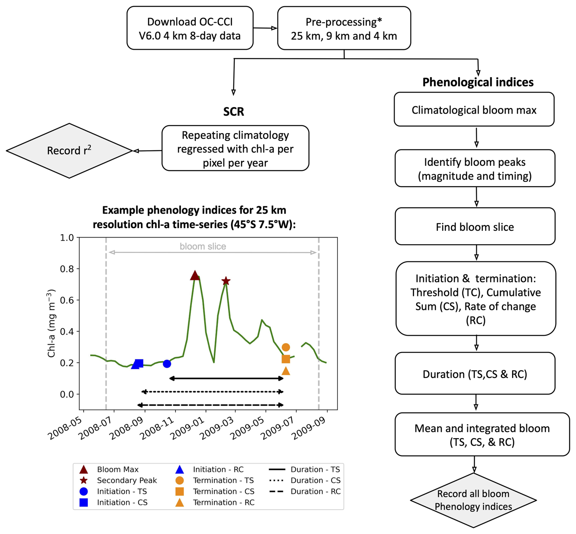
Figure 1 Methodological flowchart outlining the steps taken to calculate the phytoplankton seasonal metrics. An example time series from ocean colour satellite observations from OC-CCI illustrating the performance of the resulting phenological indices for a bimodal (double peak) bloom in the Southern Ocean (45° S, 7.5° W) is provided for the three different phenological methods: biomass-based threshold (TS), cumulative sum (CS), and rate of change (RC). ^* See Methodology for pre-processing steps.

2.2 Phenological indices and detection

Phytoplankton blooms typically manifest as a seasonal cycle, with a bloom initiation that identifies the timing of the ramp-up in phytoplankton growth and biomass accumulation followed by bloom peaks within the growing season (which could be multiple) and finally the bloom termination, which defines the end of the growing season. The phenological indices applied here are based on those applied to the Southern Ocean in Thomalla et al. (2023). To calculate the phenological indices for initiation and termination, we apply three main detection methods used by the community (e.g. Brody et al., 2013; Ji et al., 2010), which are detailed below (iii and iv). Each detection method has its strengths and weaknesses, and therefore the choice of method for application can be determined by the user needs, which are elaborated on in Brody et al. (2013). These methods were chosen over other approaches (e.g. Platt et al., 2009; Rolinski et al., 2007) due to the method's suitability for estimates across global scales as it is capable of encompassing a wide range of different shapes in phytoplankton blooms (Racault et al., 2012). Below we outline the series of steps implemented for estimating the global phenological indices and provide an accompanying flowchart (Fig. 1) to illustrate the succession of steps being implemented. In addition, we provide some example applications at four key observing stations (Fig. A1 in the Appendix) to facilitate a visualisation of the derived phenological indices from four annual time series.

• i.

  Bloom maximum climatology. The climatological peak (maximum amplitude) of the bloom was identified as the local maximum in chl a occurring within each grid cell's 25-year climatology. This approach was necessary because the timing of bloom events varies globally: Southern Hemisphere blooms typically occur during austral spring–summer (September–February), while Northern Hemisphere blooms occur in boreal spring–summer (April–August) (Racault et al., 2012). Furthermore, both hemisphere tropics tend to be approximately 6 months out of phase with both hemisphere higher-latitude regions. As such, it would be inappropriate to use a fixed date period (or “bloom slice”; see below) to identify bloom occurrence on global scales. Instead, for each grid cell we calculate the 8 d mean climatology. The date of the maximum climatological bloom for each pixel is then used to centre the timing of the phenology detection methods described below.

• ii.

  Identification of bloom peaks. For every pixel on a year-by-year basis, we take the climatological bloom maximum peak ± 6 months and determine the date and magnitude of the bloom maximum peak for each year. To ensure that seasonal blooms with more than one peak could be accounted for, multiple bloom peaks were defined as a second, third, or nth local maxima where the chl-a concentration reached at least 75 % of the amplitude of the bloom maximum peak magnitude and were a minimum of 24 d (i.e. 3×8 d time intervals) away from the bloom maximum peak for that year. The 75 % threshold was chosen to identify peaks with similar magnitude to the bloom maximum peak so as to allow for the occurrence of a multiple-peak growing season. Choosing a threshold higher than this would likely exclude recognisable bloom peaks (which could lead to an underestimation of the bloom duration), while choosing a lower threshold may include sub-seasonal variability and lead to an overestimation of the bloom duration. These additional peaks were found within ±6 months of the maximum peak. An example of such a multi-peak bloom detection is provided in Figs. 1 and A1c. The additional peaks were identified with the Python SciPy (Virtanen et al., 2020) function find_peaks.

• iii.

  The “bloom slice”. The bloom slice, used to find the bloom initiation and termination dates, is identified for each pixel as the 6-month time span preceding and following from the maximum bloom peak (ii) or, in the case of multi-modal blooms, 6 months preceding the first and following the last peak respectively.

• iv.

  Bloom initiation. The bloom initiation date for each bloom slice as described in (iii) is calculated as the first date before either the bloom maximum or the first peak in the event of multi-modal blooms, according to the thresholds listed below.

  • 1.

    Biomass-based threshold method (TS). First determine the range as the difference in chl-a concentration between the bloom maximum and preceding minimum. Then identify the bloom initiation as the first date that the chl-a concentration was greater than the minimum chl-a concentration plus 5 % of the chl-a range.

  • 2.

    Cumulative biomass-based threshold method (CS). First remove any values preceding the bloom slice minimum chl-a concentration and any values greater than 3 times the median of the bloom slice, before calculating the cumulative sum of chl a. Then identify the first date that the chl-a concentration was greater than 15 % of the total cumulative chl-a concentration.

  • 3.

    The rate-of-change method (RC). First determine the rate of change of the bloom slice and then identify the first date after the minimum that the chl-a rate of change was greater than 15 % of the median rate of change in chl-a concentration.

  Of note, the choice of above chosen percentage thresholds is in accordance with those used by previous phenological detection studies (Brody et al., 2013; Hopkins et al., 2015; Ji et al., 2010; Thomalla et al., 2011, 2015, 2023).

• v.

  Bloom termination. The bloom termination date for each bloom slice was similarly calculated to the first date after the bloom maximum or the last peak in the event of multi-modal blooms, according to the thresholds below.

  • 1.

    TS is the first date that the chl-a concentration was less than the minimum chl-a concentration plus 5 % of the chl-a range.

  • 2.

    CS is the first date between term peak and post-bloom minimum that the chl-a concentration was less than 15 % of the total cumulative chl-a concentration.

  • 3.

    RC is the first date between term peak and post-bloom minimum that the chl-a rate of change was less than 15 % of the median rate of change in chl-a concentration.

• vi.

  Bloom duration. The bloom duration was calculated as the number of days between the bloom initiation and termination dates. This is applied to each phenological detection method described above (TS, CS, and RC).

• vii.

  Integrated and mean bloom chl a. The seasonally integrated bloom chl a was calculated using the NumPy (Harris et al., 2020) trapezoidal function as the chl-a concentration integrated between the bloom initiation and termination dates. The seasonal mean chl a was calculated as the average chl a between the bloom initiation and termination dates. These are applied to each of the three phenological detection methods described above (TS, CS, and RC).

• viii.

  SCR. The variance of the seasonal cycle was calculated as defined in Thomalla et al. (2023), where the SCR is the Pearson's correlation coefficient of the annual seasonal cycle correlated against the climatological mean seasonal cycle. A value of 100 % is indicative of an annual seasonal cycle that is a perfect repetition of the climatological mean, while a value of 0 % means that there is no annually reproducible mean seasonal cycle. Unlike for phenological indices i–vii, for SCR the original OC-CCI v6.0 data were used for the three different grid resolutions, however with only spatial-temporal interpolation for gap filling and no rolling mean to avoid smoothing out temporal variability. For SCR for each pixel the bloom slice is restricted to 12 months (i.e. January to December).

The cyclical nature of the calendar presents a significant challenge when calculating means and standard deviations of phenological indices. For example, we need to avoid a situation where the mean bloom initiation between a year with a bloom in December (day of year = 340) and a year with a bloom in January (day of year = 10) is incorrectly calculated as an average bloom initiation date in July (day of year = 175). To address this, as similarly applied in Thomalla et al. (2023), we used the Python SciPy function circmean (or circstd for standard deviation), which calculates circular means for samples within a specified range, correctly identifying the mean as day of year 357. The user should also be aware that any pixels in the first year of this satellite-derived data product where the initiation date is the same as the first available start date of chl a (e.g. 4 September 1997) should be masked out. Similarly, any pixels in the last year of the product where the termination date is the same as the last available chl-a time step (e.g. 27 December 2022) should be masked out.

3 Results and discussion

3.1 Global open-ocean phytoplankton seasonal metrics

A significant degree of regional variability is evident in the mean distribution of seasonal metrics (bloom amplitude, timing, and seasonality) (Fig. 2). Bloom magnitude metrics (maximum bloom chl a, mean bloom chl a, and integrated bloom chl a; Fig. 2a–c) are all higher in the high latitudes and in the coastal regions, particularly in the eastern boundary current systems, and lowest in the oligotrophic subtropical gyres. There is a general Equator-to-pole symmetry in the timing of phytoplankton blooms between the Northern Hemisphere and the Southern Hemisphere. In the subpolar regions phytoplankton blooms initiate in the northern hemisphere during boreal spring to early summer (March–May) and in the Southern Hemisphere in austral spring to early summer (September–November) in response to light availability (Sverdrup, 1953) (Fig. 2d). While in the subtropics, where there is ample light throughout the year, blooms typically initiate in autumn to winter in response to nutrient supplies through winter-driven deepening of the mixed layer (Fauchereau et al., 2011; Thomalla et al., 2011). In both the Antarctic and Arctic polar regions, phytoplankton blooms initiate in austral (December) and boreal summer (July), when the sea ice cover melts. The timing of bloom maximum follows a similar Equator-to-pole symmetry to bloom initiation (Fig. 2g), with high-latitude regions peaking in austral and boreal summer, whereas the subtropics peak in austral and boreal winter. This large-scale meridional structuring of the bloom timing is as expected and similarly found in previous large-scale satellite-based phenological studies (Kahru et al., 2011; Racault et al., 2012; Sapiano et al., 2012). There is a larger degree of spatial heterogeneity in bloom termination (Fig. 2e), particularly evident in regions such as the high-latitude North Atlantic and sub-Antarctic, with terminations that extend up to 6 months later in comparison to surrounding areas which were initiated at a similar time. This manifests in zonal asymmetries across the different basins for bloom duration (Fig. 2f), with considerably longer blooms occurring in the Pacific Basin compared with the Atlantic and Indian basins. SCR covers a large range of variability across latitudinal bands. Notably, SCR (Fig. 2h) is oftentimes low in regions where bloom duration is long, and this relationship is strongest in the tropical Pacific ($r\sim -\mathrm{0.4}$). In these oligotrophic regions, where bloom amplitude is constrained by nutrients, the seasonality of phytoplankton blooms is not well defined and characterised by high intraseasonal variability (Fig. 2, Thomalla et al., 2011). Worth noting when applying our bloom detection method to these regions is that it does not constrain a bloom slice to be within a 12-month period, as is done in other phenology studies (e.g. Henson et al., 2018). Rather, by allowing for multiple peaks to be considered within a bloom, this approach may produce extended bloom durations that are beyond a year in regions with no discernable or strongly defined seasonal cycle. In the Southern Ocean, with higher bloom amplitudes and a well-defined yet highly variable seasonal cycle, sustained blooms of ∼ 250 d are detected, which have been attributed to intermittent physical forcing (high-frequency wind and meso- to submesoscale dynamics) that entrains nutrients and prolongs the seasonal termination (Thomalla et al., 2011, 2023).

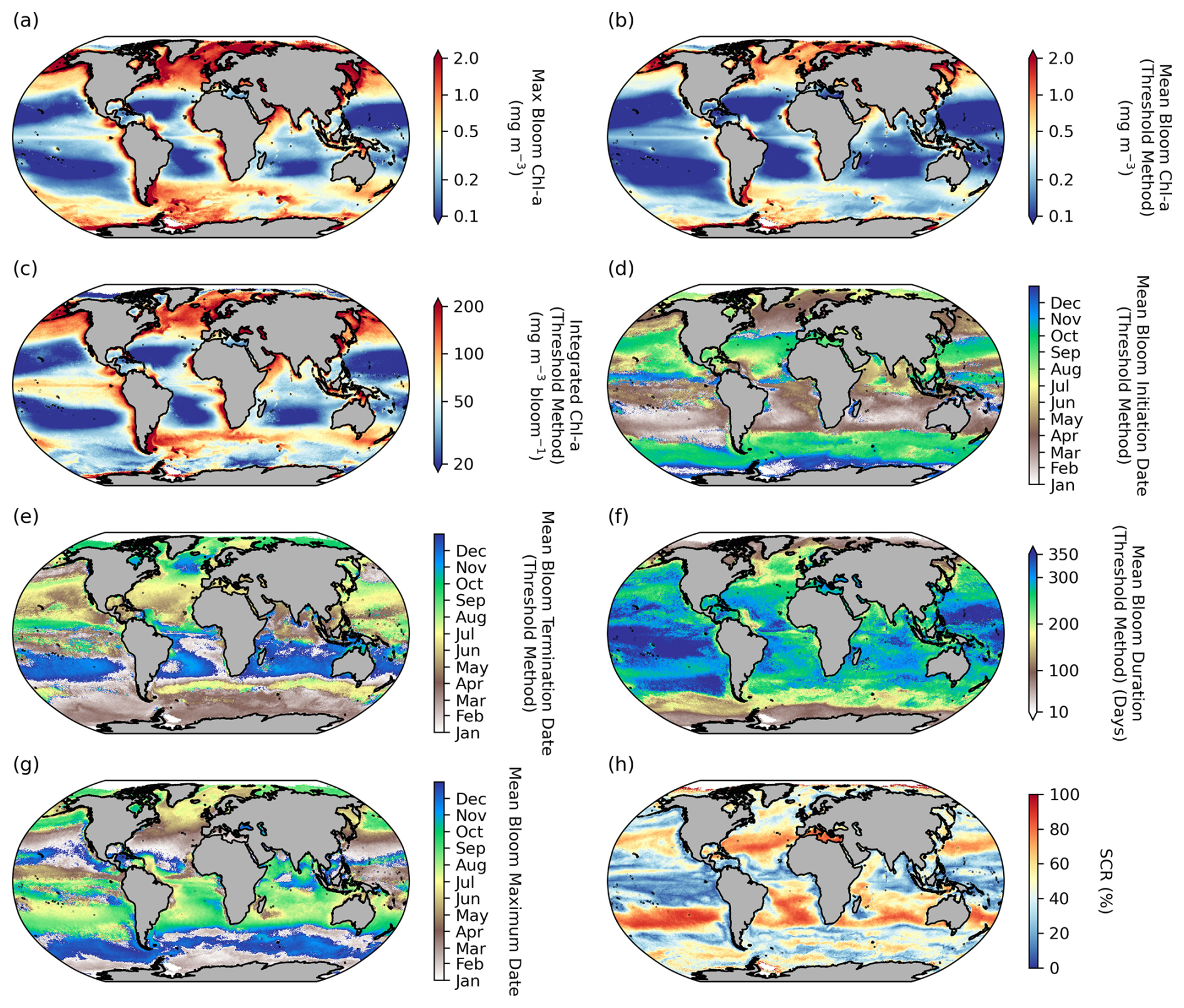
Figure 2 Global distribution of phytoplankton seasonal metrics. Mean (1998–2022) maps of (a) bloom maximum chlorophyll a (chl a), (b) mean chl a over bloom duration, (c) integrated chl a over bloom duration, (d) bloom initiation, (e) bloom termination, (f) bloom duration, (g) bloom maximum chl-a date, and (h) seasonal cycle reproducibility (SCR). Phenological indices (b–f) are determined using the biomass-based threshold method as defined in Henson et al. (2018) and Thomalla et al. (2023).

A comparison of our satellite-derived phenology product with bloom indices derived from in situ data at a selection of regional case studies shows reasonable agreement. For example, in the Saronikós Gulf (eastern Mediterranean), Kalloniati et al. (2023) report a mean bloom initiation in early October (2005–2015), which compares well with our mean bloom initiation over the same period of 24 September. Similarly, their mean bloom peak occurs in late February, closely matching our estimate of 24 February. However, there are notable differences in bloom termination with their approach reporting a seasonal bloom that terminates in mid-April, compared to our estimate of ∼ 100 d later on 13 July. This discrepancy likely arises because their method does not account for multiple bloom peaks, whereas our method is specifically designed to include the secondary peak observed in April as part of the seasonal bloom (see their Fig. 3c). Another example from long-term mooring observations (1998–2022) in the Bering Sea shelf (Nielsen et al., 2024) reports the timing of the bloom maximum to range annually between the end of April to mid-June (see their Fig. 2), which compares well with our mean estimate over the same period of 25 May (standard deviation of 57 d). In a Red Sea comparison, although our satellite-derived phenology data product was able to detect similar bloom initiation and maximum peak timing for the primary bloom in winter (as observed by Racault et al., 2015), it is not designed to provide indices for bimodal blooms and thus is unable to identify the secondary bloom in summer. Beyond these existing studies, we applied our phenological detection method (TS) to chl-a data from the Hawaii Ocean Time-series (HOT) and Bermuda Atlantic Time-series Study (BATS) long-term monitoring sites (Fig. A2, Valente et al., 2022). At HOT, the in situ mean (1998–2018) bloom initiation was 25 July (±48 d) compared to the satellite-derived mean of 21 July (±42 d) (Fig. A2a). Similar agreement was apparent in other bloom metrics. The in situ mean bloom max timing was 12 December vs. 5 December; the termination was 22 May (±32 d) vs. 6 June (±29 d); subsequently, the mean in situ duration was 299 d vs. 303 d from satellite data. Similar agreement was seen in the BATS station (Fig. A2b).

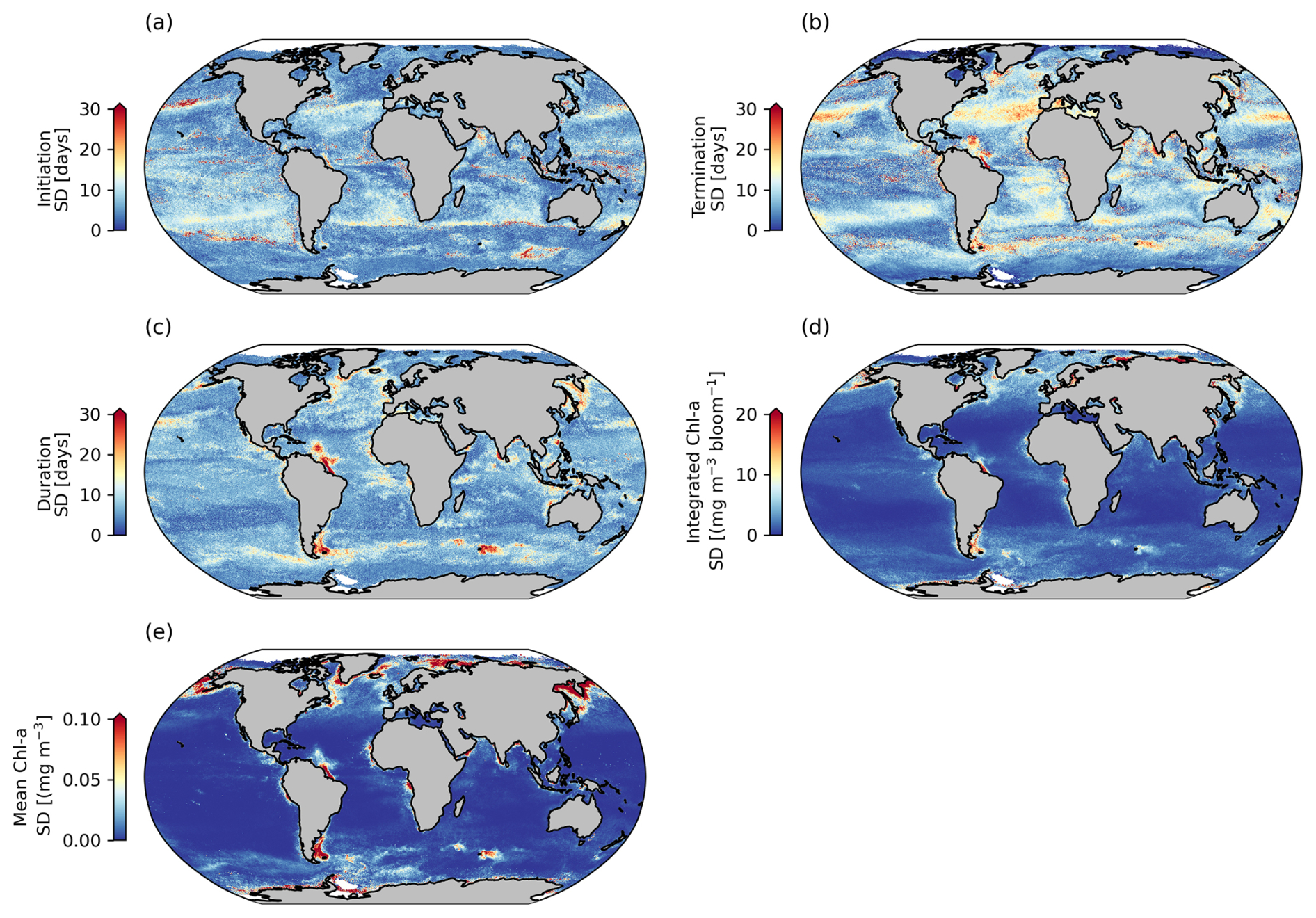
Figure 3 Comparisons between phenological detection methods. Shown are standard deviations (SDs) calculated between the biomass-based threshold method, the cumulative biomass-based threshold method, and the relative of change method, for selected seasonal phytoplankton bloom metrics, including (a) bloom initiation, (b) bloom termination, (c) bloom duration, (d) bloom-integrated chl a, and (e) bloom mean chl a.

3.2 Comparison between phenology detection methods

Phytoplankton blooms can initiate rapidly, slowly, be short-lived, intermittent, or sustained over a growing season, with different detection methods being more or less sensitive to these varying characteristics of the seasonal bloom (Brody et al., 2013; Ji et al., 2010; Thomalla et al., 2023). In this satellite-derived data product we have chosen to provide three widely used bloom detection methods for all three resolutions, allowing the user to determine which method (or all) is most appropriate for their region and application (Figs. 3 and A3). Indeed, these methods each have their strengths and weaknesses. For example, as explained in Brody et al. (2013), the biomass-based TS method will likely capture the bloom start dates at the largest increase in chl-a concentrations. It is thus more suitable for studies wanting to investigate the match or mismatch between phytoplankton and upper trophic levels as the match–mismatch hypothesis is based on the timing of the high-phytoplankton-biomass period (Cushing, 1990). This method has been found to be relatively insensitive to the percentage of the threshold used (Brody et al., 2013; Siegel et al., 2002). The RC method, which identifies the bloom initiation as the time when chl a increases rapidly, is likely more suitable for investigating the physical or biochemical mechanisms that create conditions in which the bloom occurs (Brody et al., 2013). Whereas the CS method could be used to identify either of the features above, Brody et al. (2013) showed that, while there are sensitivities of the CS method to the threshold chosen, the 15 % threshold as applied here is most appropriate at capturing bloom initiation dates of both subpolar and subtropical regions and thus most appropriate to be applied across global scales. It is interesting and potentially valuable to determine when and where different methods of determination agree or disagree, and we advocate for users to apply all three methods so that they may interrogate the differences and make informed decisions about choosing one over another or utilising all three to define a range in the desired metric. In Fig. 3, the standard deviation (SD) between the three methods is applied globally to assess the agreement between climatological means from the different methods.

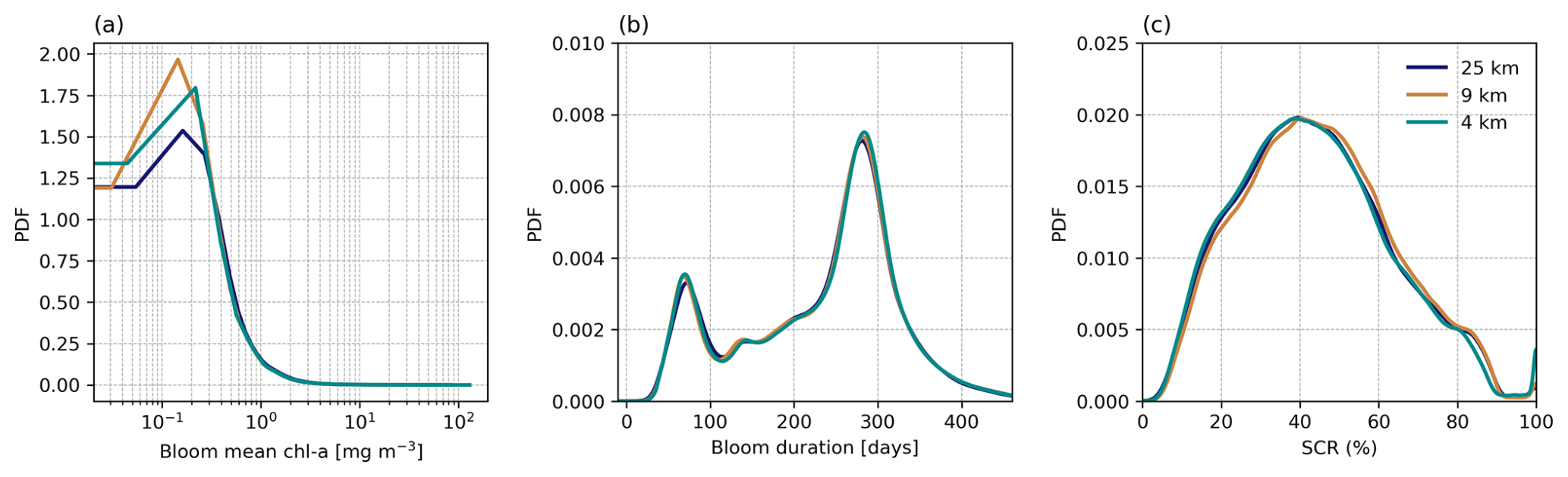
Figure 4 Probability density functions (PDFs) of climatological mean (calculated from 1998 to 2022) phytoplankton seasonal cycle metrics, compared across three different spatial resolutions (4, 9, and 25 km) for (a) bloom mean chlorophyll a (chl a), (b) bloom duration, and (c) seasonal cycle reproducibility (SCR). The TS phenology method is used for (a) and (b).

Across large regions of the global ocean, there is good agreement between the different methodological approaches (e.g. the global mean SD for the phenological timing indices is ∼ 8 d) (Fig. 3a–b). All methods produce similar large-scale patterns (Fig. A3a–c, g–f, m–o). There are however some specific regions where larger differences in timing emerge of ∼ 30–50 d (Figs. 3 and A3d–f, j–l), which are of a similar order of magnitude to that reported by Brody et al. (2013), who found areas with differences exceeding 2 months. The largest differences for both bloom initiation and termination tend to coincide with transitional zones such as at the boundaries between the subtropical and subpolar gyres in both hemispheres and in all three basins (Fig. 3a, b). This is not too surprising, given that these boundaries represent areas of significant biogeochemical signatures and regime shifts between phytoplankton seasonal characteristics with strong north–south gradients in bloom metrics (Fig. 2). While there are no other comparisons of these detection methods on a global scale, such differences were similarly seen in Brody et al. (2013) for the North Atlantic bloom, their Fig. 4, where the largest differences between bloom initiation methods occurred at the sharp transition boundaries between the subtropical and subpolar latitudes. In general, there is stronger agreement between methods in the higher subpolar latitudes compared to subtropical latitudes, as evidenced by slightly elevated SDs in the subtropical gyres (Fig. 3a, b). The subtropical oligotrophic regions are characterised by phytoplankton seasonal cycles that typically have lower bloom amplitudes, are more gradual, and have longer durations (Fig. 2). The TS method tends to produce earlier bloom initiations and earlier terminations in these subtropical regions (Fig. A3d–e, j–k). In these regions the chl-a minimum–maximum range is relatively small; thus a 5 % threshold may be exceeded earlier in both termination and initiation. The RC method, based on the rate of change, is likely to produce later bloom timing dates in more gradual blooms. There is agreement in the resultant bloom durations between the different methods, with similar large-scale patterns being reproduced by all three methods (Figs. 3c, A3m–o). Unsurprisingly, in the oligotrophic regions, differences between the methods in bloom duration do not translate to large differences in the integrated and mean bloom chl a because of the low magnitude of the chl a (Figs. 2a–c, 3c–e). There are, however, corresponding regions with more noteworthy disagreements in both duration and mean and integrated bloom chl a, for example in the energetic regions of the Antarctic Circumpolar Current, particularly near sub-Antarctic islands, and localised coastal regions with significant river runoff, such as in the Atlantic where the Amazon River discharge occurs. These areas of large SDs between the methods are driven predominantly by the TS method (Fig. A3p–r), which tends to result in shorter blooms, due to later initiations and earlier terminations (Fig. A3d, e, j, k).

3.3 High-resolution phenology indices

The derived phenology data product presented here is offered at three different horizontal resolutions (4, 9, and 25 km), which when compared on a global scale (Fig. 4) shows little to no difference in the overall mean distribution of three selected phytoplankton seasonal metrics, including bloom mean chl a (Fig. 4a), bloom duration (Fig. 4b), and SCR (Fig. 4c). Given that the large-scale distributions of the seasonal metrics remain virtually the same, there is little benefit for the user to use the more computationally expensive 4 km product for applications across these larger scales.

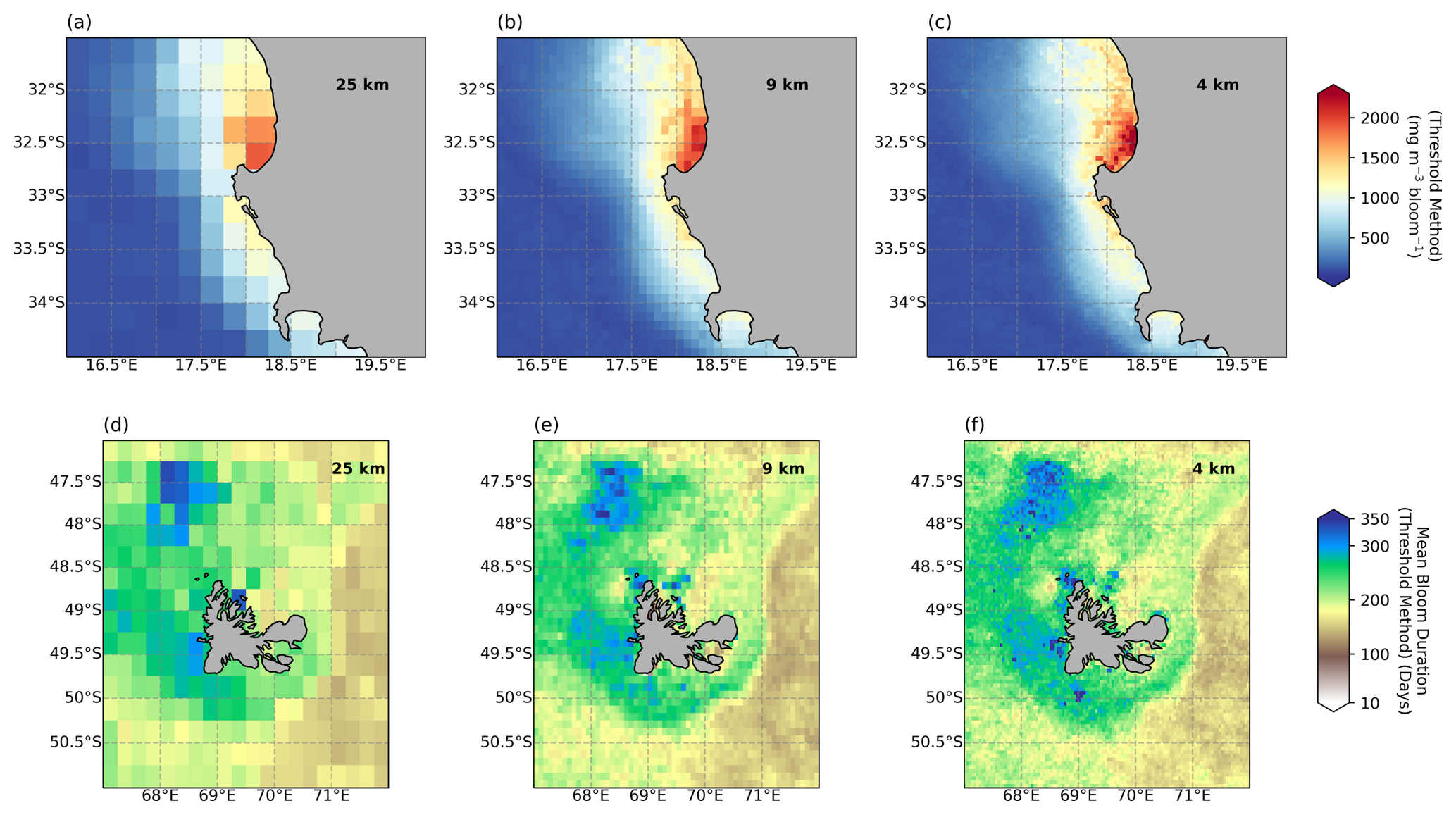
Figure 5 Regional domains comparing the impact of different resolutions: (a, d) 25 km, (b, e) 9 km, and (c, f) 4 km on (a–c) bloom-integrated chl a and (d–f) the bloom duration averaged from 2017–2022 for (a–c) the Benguela upwelling system, off the west coast of South Africa, and (d–f) the Kerguelen Islands, a sub-Antarctic island group in the Southern Ocean.

There are, however, notable differences in the resolution of the product on smaller regional scales which appear qualitatively different when compared at two example sites (Fig. 5). The sites were selected to reflect regions where a critical dependence is anticipated on the timing and magnitude of seasonal phytoplankton production. The Benguela upwelling system (Fig. 5a–c), off the west coast of South Africa, is an essential region for supporting key fisheries, while the sub-Antarctic Kerguelen Islands (Fig. 5d–f) are a vulnerable marine ecosystem that supports a number of key species. The coarseness of the 25 km product is clearly evident in both sites at these scales, it is considerably more pixelated, and there are notable patches where there are differences in the resultant phenological metric between resolutions. For example, in the nearshore of Saint Helena Bay the integrated bloom chl-a climatology (2017–2022) differs between resolutions from 1654, 1841, and 1843 mg m⁻³ per bloom, for the 25, 9, and 4 km maps respectively, representing a ∼ 10 % underestimation by the 25 km product. At the Kerguelen Islands, the interaction of the polar front with shallow bathymetry generates persistent fine-scale ocean dynamics that set strong regional gradients in phytoplankton production (Park et al., 2014). These fine-scale gradients are clearly seen in the spatial variability of bloom duration captured by the higher-resolution products. The “footprint” of the islands is evident in the extended bloom durations occurring over the shallow plateau associated with the islands where there is considerable resuspension of dissolved iron, a key limiting nutrient (Blain et al., 2001). These examples highlight how this data product can be applied to derive valuable indicators for use in national biodiversity assessments, pelagic ecosystem mapping, and marine resource management with the added potential of monitoring change in climate sensitive regions relevant for ecosystem services. For regional studies or applications in coastal domains, it is recommended that users favour the high-spatial-resolution product, as it could facilitate detection of finer-scale delineations of phenoregions in transitional waters or detect fine-scale distributions in phenology metrics that are associated with physical or oceanographic features such as eddies, bays, and upwelling cells. While some phenology indicators produced from daily data could offer additional insights into coastal regions with high temporal variability (e.g. Ferreira et al., 2021), our data set offers a resource for areas where long gaps in the time series could negate the use of daily data.

4 Limitations of the phenology algorithm and future developments

The diversity of the phytoplankton seasonal cycles across the global ocean makes it challenging to generalise a single methodological approach that is capable of capturing all phenological metrics accurately. Our attempt to do so with this data product may lead to some irregularities, most notably when applied to regions with a poorly defined or unique seasonal cycle. For example, in ultra-oligotrophic regions where the bloom amplitude is particularly low and intraseasonal variability particularly high, our detection method prescribes long bloom durations that may exceed 1 year and can lead to overlapping bloom slices. Another example is regions with bimodal blooms, where there is a well-defined summer and winter bloom in a given annual cycle. Although our phytoplankton phenology detection method is designed to allow for multiple peaks to occur within a bloom cycle, it has not been designed to cater to bimodal annual cycles, which would require the identification of separate summer and winter initiation and termination indices. In these instances our method may result in extended bloom durations. While these regions are relatively uncommon (e.g. Racault et al., 2017; Fig. 2c), they do exist, as is the case with the Red Sea (Racault et al. 2015). Future developments of this data product will endeavour to incorporate updates and improvements to the detection methods to better cope with these irregularities. We welcome users to reach out if other irregularities are identified within a specific area of interest and to work with the authors to improve future versions of the product. All future changes to the product will be fully documented on Zenodo as new versions are released.

5 Code and data availability

The data are available on the Zenodo repository under the following DOIs: https://doi.org/10.5281/zenodo.8402932 for 4 km, https://doi.org/10.5281/zenodo.8402847 for 9 km, and https://doi.org/10.5281/zenodo.8402823 for 25 km (Nicholson et al., 2023a, b, c). Chl-a data, used to develop the phytoplankton phenology product, are available from the Ocean Colour–CCI data set (v.6.0) at https://doi.org/10.5285/5011d22aae5a4671b0cbc7d05c56c4f0 (Sathyendranath et al., 2023). The code used to produce the figures of this article can be found at https://github.com/sarahnicholson/global_phytoplankton_phenology (last access: 2 May 2025) and https://doi.org/10.5281/zenodo.15323392 (Nicholson et al., 2025).

6 Conclusions

The satellite-derived data product presented here provides a 25-year continuous record of key phytoplankton seasonal cycle metrics (phytoplankton bloom phenology, bloom seasonality, and bloom magnitude) on a global scale. It includes three different phenology detection methods that are widely used by the community. We do not advocate for a particular method over another. The strengths and weaknesses of these different approaches have been highlighted in other studies (e.g. Brody et al., 2013). It is up to the user to choose which (if not all) is the most appropriate for their research application. The data product is also provided at three different horizontal resolutions (4, 9, and 25 km) for regional- versus global-scale application. This product is applicable for a broad range of national to international research and industry applications. Its primary strength is that it can be used to assess, monitor, and understand regional- to global-scale characteristics in phytoplankton phenology and to detect change associated with environmental drivers, which is critical for effective management of marine ecosystems and fisheries. This data product will undergo regular updates for future applications and extended time series analysis, which typically happens every 2 years. It will also be updated when data are temporally extended or when the OC-CCI releases any version updates beyond v.6.0 that include backwards corrections for previous years, so the entire data set aligns with the latest version of OC-CCI. This helps to prevent the retention of erroneous values within the data set.

Appendix A

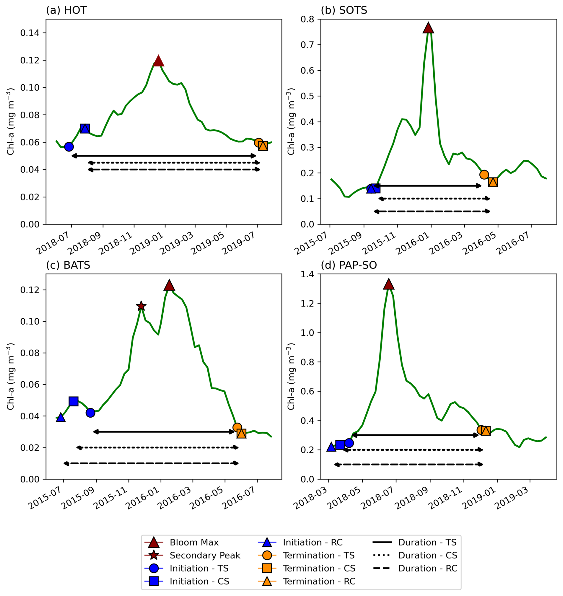
Figure A1 Examples of phytoplankton bloom seasonal cycles of satellite-derived chlorophyll a from OC-CCI and comparisons in phenological detection methods at key sustained observing stations across the global ocean. For (a) the Hawaii Ocean Time-series (HOT; 21°20.6^′ N, 158°16.4^′ W), (b) the Southern Ocean Time Series Observatory (SOTS; 140° E, 47° S), (c) the Bermuda Atlantic Time-series Study (BATS; 31°50^′ N, 64°10^′ W), and (d) the Porcupine Abyssal Plain (PAP-SO; 49° N, 16.5° W) sustained observatory time series.

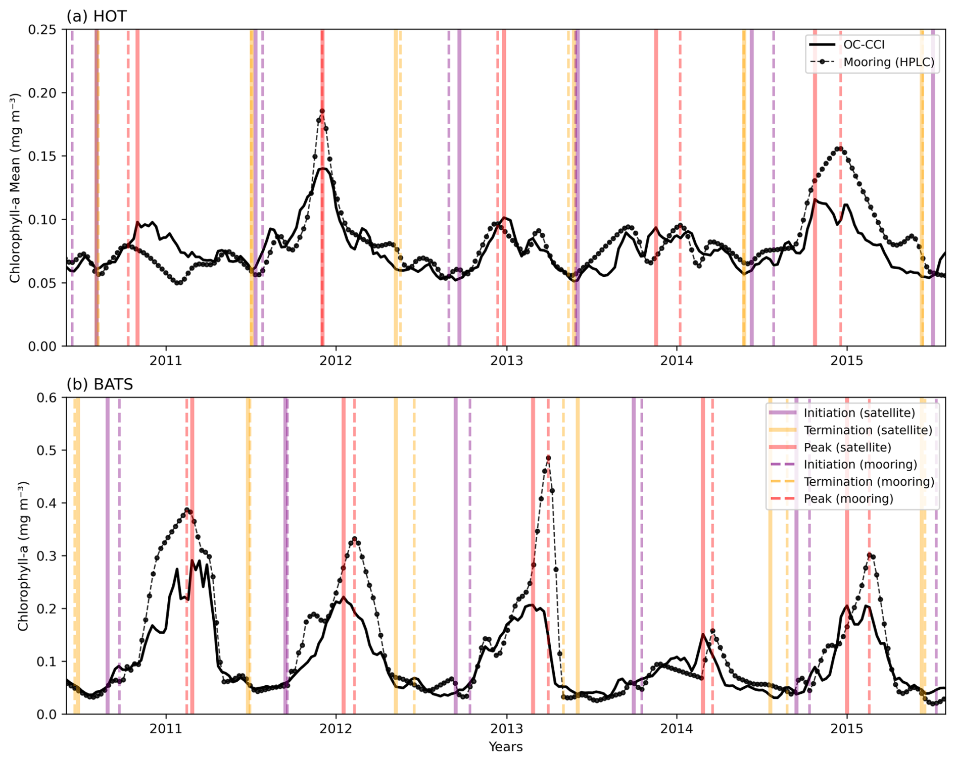
Figure A2 Comparison of 5 years of in situ chlorophyll-a measurements (Valente et al., 2022) with satellite-derived chlorophyll a (OC-CCI), along with key phenological indices (solid and dashed vertical lines for satellite and mooring respectively) at two sustained observing stations: (a) the Hawaii Ocean Time-Series (HOT; 21°20.6^′ N, 158°16.4^′ W) and (b) the Bermuda Atlantic Time-series Study (BATS; 31°50^′ N, 64°10^′ W).

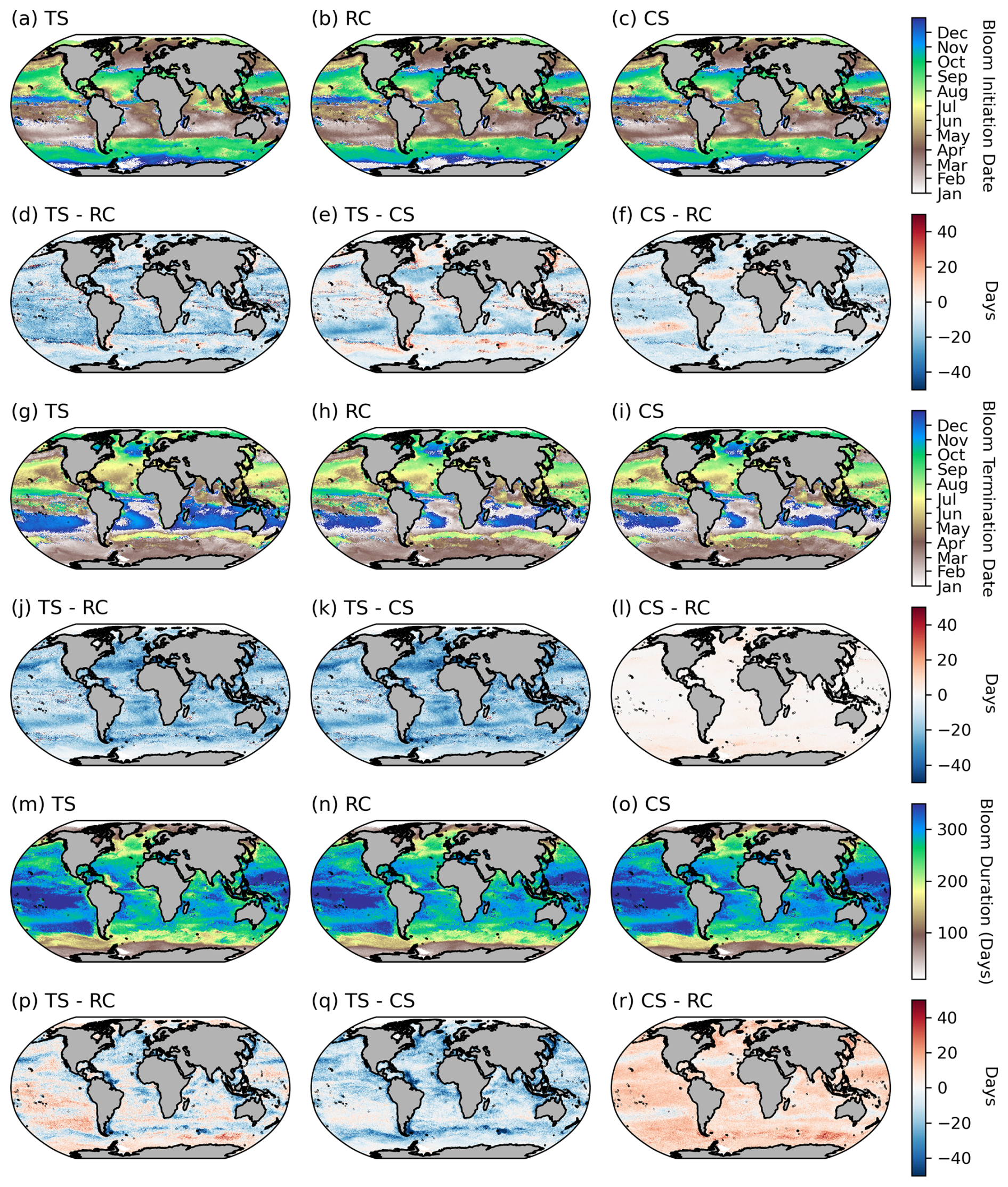
Figure A3 Comparisons between phenological detection methods. The climatological means (1998–2022) for (a–c) bloom initiation, (g–i) bloom termination, and (m–o) bloom duration. The differences between the climatological means for the biomass-based threshold method (TS), the cumulative biomass-based threshold method (CS), and the rate-of-change method (RC) are provided for bloom initiation (d–f), bloom termination (j–l), and bloom duration (p–r).