GHOST: a globally harmonised dataset of surface atmospheric composition measurements

GHOST (Globally Harmonised Observations in Space and Time) represents one of the biggest collections of harmonised measurements of atmospheric composition at the surface. In total, 7 275 148 646 measurements from 1970 to 2023, of 227 different components from 38 reporting networks, are compiled, parsed, and standardised. The components processed include gaseous species, total and speciated particulate matter, and aerosol optical properties.

The main goal of GHOST is to provide a dataset that can serve as a basis for the reproducibility of model evaluation efforts across the community. Exhaustive efforts have been made towards standardising almost every facet of the information provided by major public reporting networks, which is saved in 21 data variables and 163 metadata variables. Extensive effort in particular is made towards the standardisation of measurement process information and station classifications. Extra complementary information is also associated with measurements, such as metadata from various popular gridded datasets (e.g. land use) and temporal classifications per measurement (e.g. day or night). A range of standardised network quality assurance flags is associated with each individual measurement. GHOST's own quality assurance is also performed and associated with measurements. Measurements pre-filtered by the default GHOST quality assurance are also provided.

In this paper, we outline all steps undertaken to create the GHOST dataset and give insights and recommendations for data providers based on the experiences gleaned through our efforts.

The GHOST dataset is made freely available via the following repository: https://doi.org/10.5281/zenodo.10637449 (Bowdalo, 2024a).

1 Introduction

The 20th century bore witness to a revolution in scientific understanding in the atmospheric composition field. In the early 1950s, ozone (O₃) was identified as the key component of photochemical smog in Los Angeles (Haagen-Smit, 1952), and sulfur dioxide (SO₂) was identified as the key component of the “London smog” (Wilkins, 1954). These findings led to a number of clean-air laws being implemented in the most developed regions of the world (e.g. UN, 1979) and with this an explosion in monitoring activity, with measuring networks created to continuously measure the concentrations of key components. Over the next few decades the importance of particulate matter (PM) as a pollutant became better understood (Whitby et al., 1972; Liu et al., 1974; Hering and Friedlander, 1982). However, it took until the 1980s and 1990s respectively for PM exposure to be more rigorously monitored via aerodynamic size fractions, i.e. PM₁₀ and PM_2.5 (Cao et al., 2013).

In the present day we know of hundreds of atmospheric components which act as pollutants impacting human and plant health (Monks et al., 2015; Mills et al., 2018; Agathokleous et al., 2020; Vicedo-Cabrera et al., 2020) and hundreds more which directly or indirectly affect the concentrations of these components. Furthermore, some of these pollutants impact climate forcings in some capacity via direct, semi-direct, and indirect effects (Forster et al., 2021).

A critical approach for our understanding of the complex, non-linear processes which control the concentration levels of components in the atmosphere is through the use of chemical transport models (CTMs) and Earth system models (ESMs). In order to evaluate the veracity of these models, observations are required. Unfortunately, the limited availability and quality of these observations serve as a major impediment to this process. Since the 1970s, atmospheric components have been extensively measured around the world by long-term balloon-borne measurements (Tarasick et al., 2010; Thompson et al., 2015), suitably equipped commercial aircraft (Marenco et al., 1998; Petzold et al., 2015), research aircraft (Toon et al., 2016; Benish et al., 2020), ships (Chen and Siefert, 2003; Angot et al., 2022), and satellites (Boersma et al., 2007; Krotkov et al., 2017). However, each of these measurement types has drawbacks associated with the temporal, horizontal, or vertical resolution of the measurements. Near-global coverage by satellites exists for some components (e.g. CO or NO₂), but these require complex corrections and cannot yet isolate concentrations at the surface (Kang et al., 2021; Pseftogkas et al., 2022) in the air most relevant for humans and vegetation. The most temporally consistent measurements have been made at the surface by established measurement networks, although the spatial coverage of these measurements is typically limited, being predominantly located in the most developed regions.

The ultimate purposes of measurements at in situ surface stations are wide-ranging, from providing information regarding urban air quality exceedances to monitoring long-term trends or simply advancing scientific understanding of atmospheric composition. Owing to this, numerous different institutions or networks manage the reporting of this information, meaning information is reported in a plethora of different formats and standards. As a consequence, the aggregation and harmonisation of both data and metadata, from across these networks, requires extensive effort.

Efforts to synthesise measurements across surface networks have been made previously, but these have often been limited to a single compound of interest, e.g. O₃ (Sofen et al., 2016; Schultz et al., 2017). The AeroCom project represents one of the most complete efforts to create a model evaluation framework, harmonising both measurements (from satellites and the surface) and model output, although this project is solely limited to aerosol components (Kinne et al., 2006; Gliß et al., 2021). The Global Aerosol Synthesis and Science Project (GASSP) is another one that has made efforts to harmonise global aerosol measurements, in this case from the surface, ships, and aircraft (Reddington et al., 2017). An interesting approach to overcoming the limited spatial coverage of surface observations has been to create synthetic gridded observations (Cooper et al., 2020; van Donkelaar et al., 2021) by combining satellite data with CTM output and calibrating them to surface observations, although naturally this approach comes with significant uncertainties. There are existing efforts which parse near-real-time surface measurements globally (IQAir, 2024; OpenAQ, 2024; WAQI, 2024) or citizen science projects utilising low-cost sensors (PurpleAir, 2024; UN Environment Programme, 2024). However, these efforts are typically more tailored for public awareness purposes than for actual science, with few to no quality control procedures, a limited historical extent (maximum of ∼5 years), and a limited number of processed components. Rather than harmonise existing datasets, there have been other efforts to create universal standards with which measurement stations can comply. The World Meteorological Organization (WMO) (WMO, 2024b, c, d) has made significant efforts through the WMO Integrated Global Observing System (WIGOS) (WMO, 2019a, 2021) framework for this purpose. The Aerosol, Clouds and Trace Gases Research Infrastructure (ACTRIS) (ACTRIS, 2024) and EBAS (NILU, 2024) are two other examples of efforts to create extensive reporting standards. The number of measurement stations following these standards however represents a small fraction of those available globally.

There have been numerous model evaluation studies which utilise data from one or more surface measurement networks. However, there is typically little to no detail given about the methodology used in combining data and metadata from across different networks, the quality assurance (QA) applied to screen measurements, and the station classifications employed to subset stations (e.g. Colette et al., 2011; Solazzo et al., 2012; Katragkou et al., 2015; Schnell et al., 2015; Badia et al., 2017). Therefore, evaluation efforts from different groups are often incomparable and non-reproducible.

In response to this, we established GHOST (Globally Harmonised Observations in Space and Time). The main goal of GHOST is to provide a dataset of atmospheric composition measurements that can serve as a basis for the reproducibility of model evaluation efforts across the community. Exhaustive efforts are made to standardise almost every facet of provided information from the major public reporting networks that provide measurements at the surface. Unlike other major synthesis efforts, no data are screened out. Rather, each measurement is associated with a number of standardised QA flags, providing users with a way of flexibly subsetting data. Although this work focuses on surface-based measurements, GHOST was designed to be extensible, both to more surface network data and the incorporation of other types of measurements, e.g. satellite or aircraft.

This paper fully details the processing procedures that have resulted in the GHOST dataset. In Sect. 2 of this paper we outline the reporting networks contributing to this work. Section 3 details the processing used to transform native network data into the finalised GHOST dataset. Section 4 describes the temporal and spatial extent of the finalised dataset. Finally, Sect. 5 gives some insights and recommendations for data providers based on experiences gleaned through this work.

2 Contributing datasets

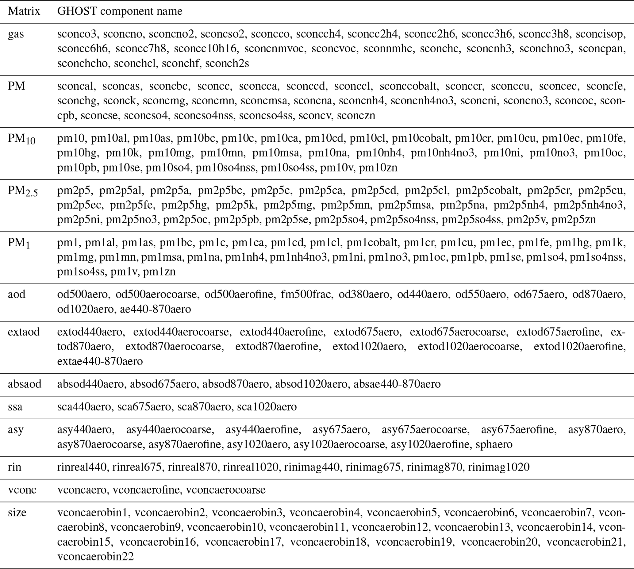
GHOST ingests data from the 38 networks listed in Table 1; 227 atmospheric components, across 13 distinct component types (or matrices), are processed by network. These matrices serve as a way of being able to more simply classify the many types of components and are, specifically, gas (all gas-phase components), PM (all particulate matter), PM₁₀ (particulate matter with a diameter ≤ 10 µm), PM_2.5 (particulate matter with a diameter ≤2.5 µm), PM₁ (particulate matter with a diameter ≤1 µm), aod (aerosol optical depth), extaod (extinction aerosol optical depth), absaod (absorption aerosol optical depth), ssa (aerosol single-scattering albedo), asy (aerosol asymmetry or sphericity factors), rins (aerosol refractive indices), vconc (aerosol total volume concentration), and size (aerosol size distribution). The components processed within GHOST are outlined per matrix in Table 2, with more detailed information given per component in Table A3.

It is important to state that the term “network” is used loosely throughout this work. Many of the “networks” that data are sourced from could be better classified as “projects”, “frameworks”, or “reporting mechanisms”. However, for the purposes of simplicity, we define “network” as the most common name for an available dataset from a specific data source. For WMO data, for example, this means that what is typically called the Global Atmosphere Watch (GAW) network is separated out across three networks, as the data are reported in a discretised form across three data centres.

The geographical coverage of the contributing networks ranges from the global to sub-national scales. The operational objectives of the networks are wide-ranging, with some of the networks set up to monitor the background concentrations of atmospheric components in rural areas (e.g. the U.S. EPA's CASTNET), whereas others exist for regulatory purposes, monitoring compliance with national or continental air quality limits (e.g. EEA AQ e-Reporting). Many of the networks have substantial, well-documented internal QA programmes.

We recognise that the datasets ingested in GHOST do not represent all of the observations of atmospheric components made globally. However, other datasets are not readily available (i.e. not available online), are unlikely to conform to the QA protocols followed by the included networks, or have too few stations to justify the time spent processing. In total, the resultant processed data collection, across all the components, comprises 7 275 148 646 measurements, beginning in 1970 with measurements from the Japan National Institute for Environmental Studies (NIES) network and going through to January 2023.

Some of the datasets come with restrictive data permissions, which typically means that redistributing the data is impossible. Through dialogue with each of the data reporters, the majority of these data are included in the public GHOST dataset. However, there are a few networks which are not able to be redistributed, which is indicated in the “Data rights” column of Table 1.

(ACTRIS, 2024)NILU (2024)NASA (2024)NASA (2024)(Arctic Council Member States, 2024)NILU (2024)BJMEMC (2024)(OSPAR Commission, 2024)NILU (2024)Canada NAPS (2024)CAPMoN (2024)Chile MMA (2024)CNEMC (2024)(COLOSSAL, 2024)NILU (2024)EANET (2024)EEA (2024a)EEA (2024b)(MET Norway, 2024; Tørseth et al., 2012)NILU (2024)(Kulmala et al., 2011)NILU (2024)(Cavalli et al., 2010)NILU (2024)(HELCOM, 2024)NILU (2024)(Gusev et al., 2012)NILU (2024)(Aas et al., 2007)NILU (2024)NILU (2024)Japan NIES (2024)SEDEMA (2024)Spain MITECO (2024)NADP (2024a)NADP (2024b)(NILU et al., 2024)NILU (2024)(NOAA-ERSL, 2024)NILU (2024)(NOAA-GGGRN, 2024)NILU (2024)(OECD, 2024)NILU (2024)UK DEFRA (2024)(University of Bristol et al., 2024)NILU (2024)US EPA (2024a)US EPA (2024b)US EPA (2024c)(WMO, 2024b)NILU (2024)WMO (2024c)(WMO, 2024d)NILU (2024)

Table 1 General descriptions of the reporting networks from which data are sourced in GHOST. For each network, the temporal extent of the processed data, the available matrices of the processed components, the data source from which the original data were downloaded, and an indication of whether the data rights of the network permit the data to be redistributed as part of the GHOST dataset are given.

Table 2 Names of the standard components processed in GHOST, grouped per data matrix. The “sconc” prefix is used for all components which can vary significantly with height. More information regarding these components can be found in Table A3.

3 GHOST processing workflow

Synthesising such a large quantity of data from disparate networks is as much a challenge from a logistical and computational processing standpoint as it is a scientific one. For this purpose we designed a fully parallelised workflow based in Python and tailored to fully exploit the resources of the MareNostrum4 supercomputer housed at the Barcelona Supercomputing Center (BSC). The workflow processes data by network and component through a pipeline of multiple processing stages described visually in Fig. 1.

There are nine stages in the pipeline, which can be grouped broadly into five different stage types: data acquisition (Stage 0), standardisation (Stages 1 and 2), data addition (Stages 3–5), temporal manipulation (Stage 6), and data aggregation (Stages 7 and 8).

There are two layers in the workflow parallelisation. Firstly, data by network and component are processed through the pipeline in parallel. Secondly, the workload at each stage of the pipeline is divided into multiple smaller jobs, which are then processed in parallel as well.

The processing in each pipeline ultimately results in harmonised netCDF4 files across all the networks by component. We will now describe the operation of each of the pipeline stages in detail.

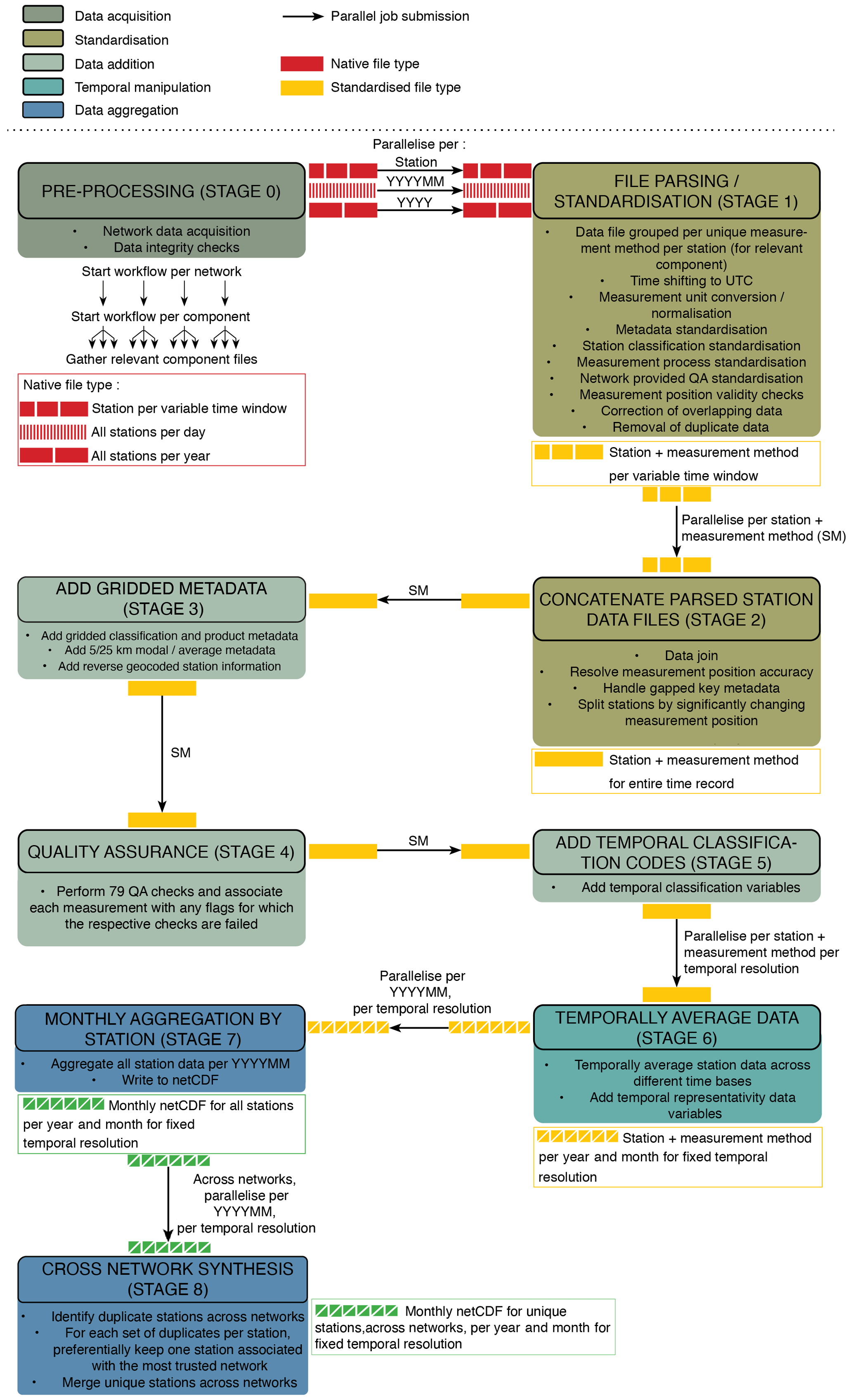
Figure 1 Visual illustration of the GHOST workflow, with data processed through a pipeline of nine different stages. There are five broad stage types: data acquisition (Stage 0), standardisation (Stages 1 and 2), data addition (Stages 3–5), temporal manipulation (Stage 6), and data aggregation (Stages 7 and 8). Data by network and component are processed through the pipeline in parallel. The workload in each individual stage is divided into multiple smaller jobs, which are also processed in parallel (the arrows between the different stages indicate the type of parallelisation). The processing in each pipeline ultimately results in harmonised netCDF4 files across all the networks by component.

3.1 Pre-processing (Stage 0)

Starting the workflow, a processing pipeline by network and component is created. Before any processing can begin, in each pipeline the relevant data for each network and component pair need to be procured and some initial checks performed to ensure the integrity of the downloaded data.

3.1.1 Data acquisition

All available measurement data between January 1970 and January 2023, from each of the 38 networks, are downloaded for the components listed in Table 2. The available data matrices, temporal extents, and data sources are outlined by network in Table 1.

The data files come in a variety of formats, with no real consistency between any of them. Inconsistencies in file formats also exist within some networks, e.g. Canada NAPS. In addition to the data files, there are often stand-alone metadata files detailing the measurement operation at each station. The formats of these files also vary considerably across the networks, and there can also be multiple files per network, e.g. EEA AQ e-Reporting.

For some networks, key details describing the measurement operation are published in network data reports or documentation. All available additional documentation across the networks was downloaded and read, greatly aiding the parsing or standardisation process described in Sect. 3.2.

3.1.2 Data integrity checks

For some networks, some basic checks are first implemented before doing any file parsing to ensure no fundamental problems exist with the data files. This is done in cases where information in the data filename and size can be used to identify potential data irregularities. For example, in the case of the EEA AQ e-Reporting network, data are reported per component, with unique component codes contained within the filenames. In some cases, the component code in the filename is not correct for the component downloaded. In such cases, these files are excluded from any further processing, although such files represent a tiny fraction of all the files.

With valid data files now gathered for the relevant network and component pair, file parsing can begin.

3.2 File parsing and standardisation (Stage 1)

In this stage, the relevant data files for a network and component pair are parsed, and the contained data or metadata are standardised. We define “data” variables as those which vary per measurement and “metadata” variables as those which are typically applicable for vast swathes of measurements, varying on much longer timescales. Upon completion of the stage, the relevant parsed data from each data file are saved in standardised equivalent files by station.

The type of parallelisation within Stage 1 is dependent on how the data files are structured. If the data files include all measurement stations per year, parallelisation is done per year. If the files include all measurement stations per day, parallelisation is done per year and month. If the data files are separate for each station per time interval, parallelisation is done per unique station.

The standardisation efforts made within GHOST are extensive and cover a number of facets. As well as harmonising the data or metadata information provided by the networks, additional information is included in the form of gridded metadata, GHOST QA flags, and temporal classification codes. The main standardisation types in GHOST are summarised in Table 3. The greater detail associated with each standardisation type is outlined in the referenced sections and summary tables, and the standard fields defined for each standardisation type are detailed in the referenced Appendix tables.

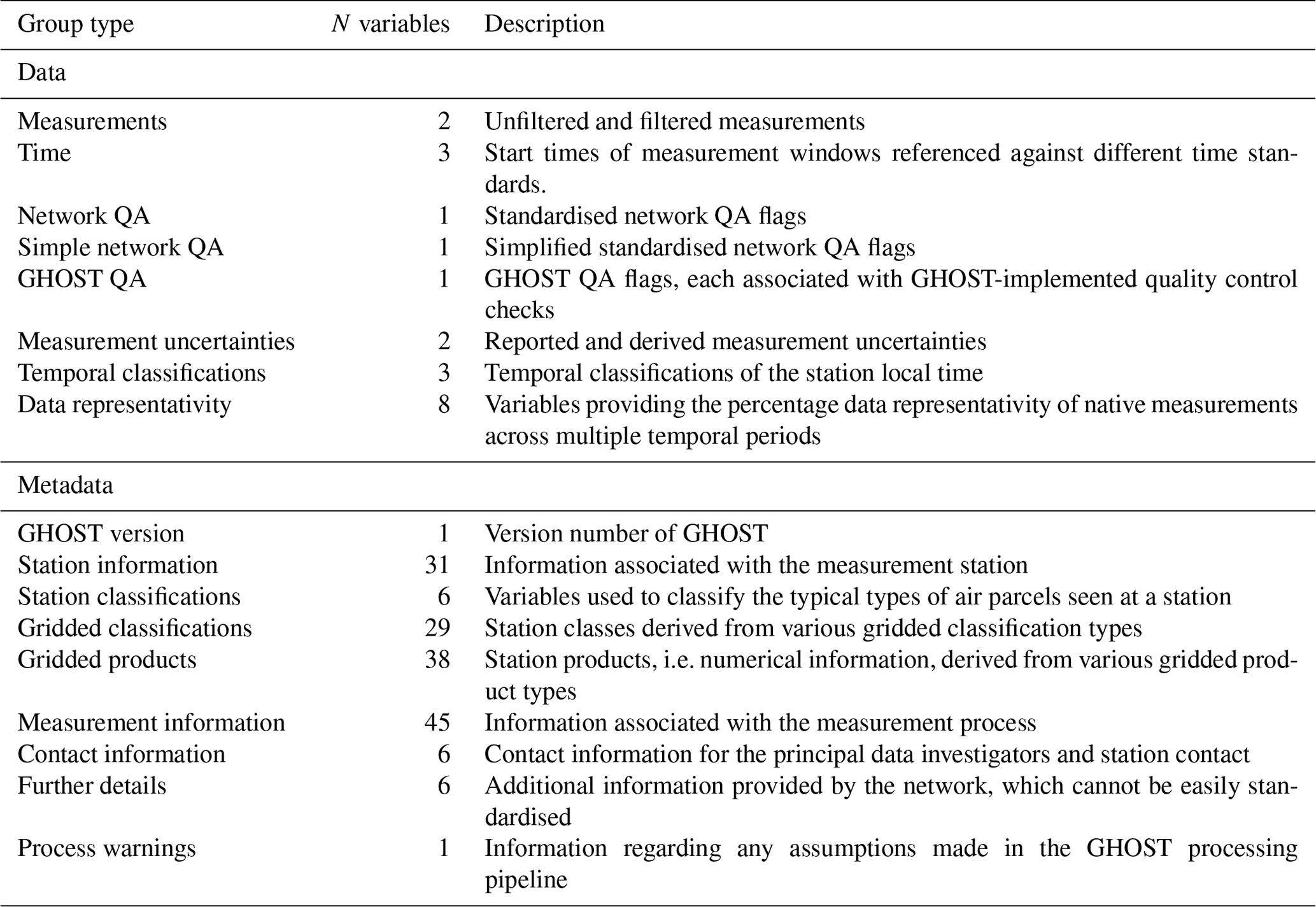
Table 4 outlines the different types of data and metadata variables standardised in GHOST. The majority of these standardisations are performed in Stage 1, with the processes involved in these standardisations described in the following sub-sections.

Table 3 Summary of the main standardisation types undertaken in GHOST. Per standardisation type, a brief description of the type, the number of variables associated with the type, the section where the type is discussed in the paper, and the numbers of the tables in the paper and Appendix outlining the type are detailed.

Table 4 Summary of the different types of data or metadata variables standardised in GHOST. For each type, a description is given, together with the total number of associated variables. Definitions of all the data or metadata variables are given in Tables A1 and A2.

3.2.1 Data grouping by station reference and measurement method

Firstly, each data file is read into memory. All non-relevant component data are removed, and a list of unique reference station IDs associated with the remaining file data is generated that henceforth is referred to as station references.

In some cases, stations operate multiple instruments to measure the same component, often utilising differing measurement methods. There can therefore be data in a file associated with the same station reference but resulting from differing measurement methods. To handle such instances, station data in GHOST are grouped by station reference and a standard measurement method. Each station group is associated with a GHOST station reference, defined as “[network station reference]_[standard measurement methodology abbreviation]”, and is saved in the GHOST metadata variable “station_reference”. The standardisation of measurement methodologies is detailed in Sect. 3.2.8.

The data in each of the station groups are then parsed independently.

3.2.2 Measured values

Measurements are typically associated with a measurement start date or time as well as the measurement end date or time or the temporal resolution of the measurement. The period between the measurement start time and end time can be termed the measurement window. In almost all cases, the measurement values reflect an average across the measurement window. Occasionally, there are multiple reported statistics per measurement window, e.g. average, standard deviation, or percentile. Only measurements which represent an average statistic are retained.

Missing measurements are often recorded as empty strings or a network-defined numerical blank code. For these cases, the values are set to “Not a Number” (NaN). Measurements for which the start time or temporal resolution cannot be established are dropped. Any measurements which do not have any associated units or have unrecognisable units are dropped. All the measurements are converted to GHOST standard units (see Sect. 3.2.13).

In the case of one specific component, aerosol optical depth at 550 nm (od550aero), the measurement is derived synthetically using several other components (od440aero, od675aero, od875aero, and extae440-870aero), following the Ångström power law (Ångström, 1929). All dependent component measurements are needed to be non-NaN for this calculation; otherwise, od550aero is set as NaN. All od550aero values are associated with the GHOST QA flag “Data Product” (code 45), and any instances where od550aero cannot be calculated are associated with the flag “Insufficient Data to Calculate Data Product” (code 46). The concept for these flags is explained in Sect. 3.2.5.

At this point, if there are no valid measurements remaining, the specific station group does not carry forward in the pipeline. If there are valid measurements, these are then saved to a data variable named by the standard GHOST component name (see Table 2), e.g. sconco3 for O₃.

3.2.3 Date, time, and temporal resolution

Some networks provide the measurement start date and time in local time, and thus a unified time standard is needed to harmonise times across the networks. We choose to shift all times to coordinated universal time (UTC), for which many of the networks already report in. For most cases where the time is not already in UTC, the UTC offset or local time zone is reported per measurement or in metadata or network documentation (i.e. constant over all the measurements). However, in the case where no local time zone information exists, this is obtained using the Python timezonefinder package (Michelfeit, 2024) as detailed in Sect. 3.4.5.

In order to store the measurement start date or time in one single data variable, it is transformed to minutes from a fixed reference time (1 January 0001, 00:00:00 UTC). Note that these units differ from the end units of the “time” data variable in the finalised netCDF4 files (see Sect. 3.7).

A small number of stations have consistent daily gaps on 29 February during leap years. An assumption is made that this is an actual missing day of data imposed by erroneous network data processing and that data labelled for 1 March are indeed for 1 March. Some networks also report measurement start times of 24:00. This is assumed to be referring to 00:00 of the next day.

For some networks, the temporal resolutions of the measurements are provided, and for others the measurement start and end dates or times are given, from which the temporal resolution can be derived. In some other cases, the temporal resolution is fixed for the entire data file, which is stated either in the filename or in the network documentation.

In some instances, the measurement start time is also not provided, with measurements provided in a fixed format, e.g. 24 h per data line, with the column headers “hour 1”, “hour 2”, etc. In these cases, there is some ambiguity as to where measurements start and stop. For example, does “hour 1” refer to 00:00–01:00, 01:00–02:00, or 00:30–01:30? An assumption is made in these cases that the column header refers to the end of the measurement window, i.e. hour 1 = 00:00–01:00. The temporal resolution of the measurements can vary widely (e.g. hourly, 3-hourly, or daily), all of which are parsed in GHOST. When later wishing to temporally average data to standard resolutions (Sect. 3.7), the temporal resolution of each original measurement is required, and therefore this information is stored through the processing.

3.2.4 Network quality assurance

Many of the networks provide QA flags associated with each measurement. These can be used to represent a number of things but are typically used to highlight erroneous data or report on potential measurement concerns. It is also often the case that one measurement is associated with multiple QA flags. Network QA flag definitions were found through the investigation of reports or documentation.

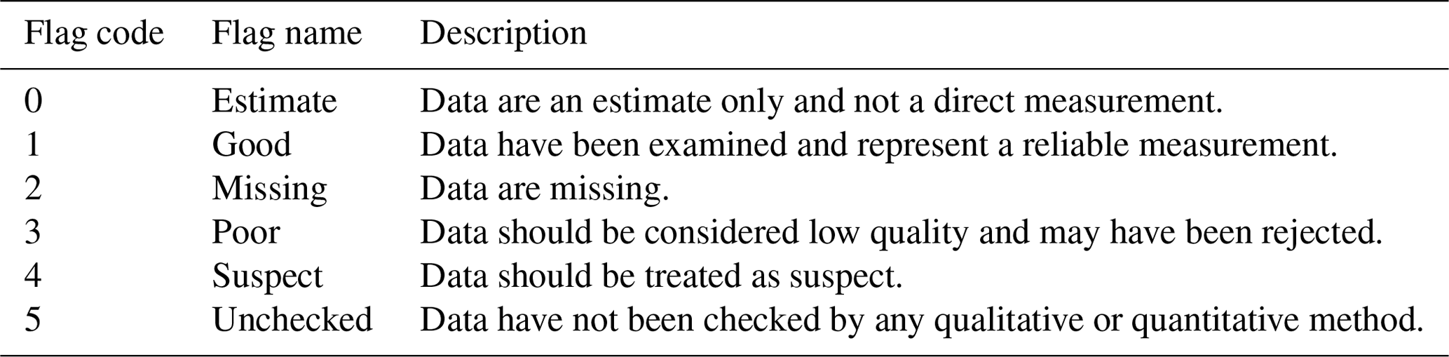
GHOST handles these flags in a sophisticated manner, mapping all the different types of network QA flags to standardised network QA flags. Table 5 shows a summary of the different types of standard flags, ranging from basic data validity flags to flags reporting on the weather conditions at the time of measurement. The standard flags are saved in the GHOST data variable “flag” as a list of numerical codes per measurement. That is, each measurement can be associated with multiple flags. Each individual standard flag name (with the associated flag code) is defined in Table A8. Whenever a flag is not active, a fill value (255) is set instead.

The large number of standard network QA flags gives the user a great number of options for filtering data, but for users who are looking to more crudely remove obviously bad measurements, the wealth of options could be overwhelming. For such cases we also implement a greatly simplified version of the standard network QA flags, defined in Table 6 and saved in the “flag_simple” variable. These definitions follow those defined in the WaterML2.0 open standards (Taylor et al., 2014). As opposed to the flag variable, each measurement can only be associated with one simple flag.

Table 5 Summary of the standard network QA flag types, stored in the flag variable. These flags represent a standardised version of all the different QA flags identified across the measurement networks. For each type, a description is given, together with the number of flags associated with each type. Definitions of the individual flags are given in Table A8.

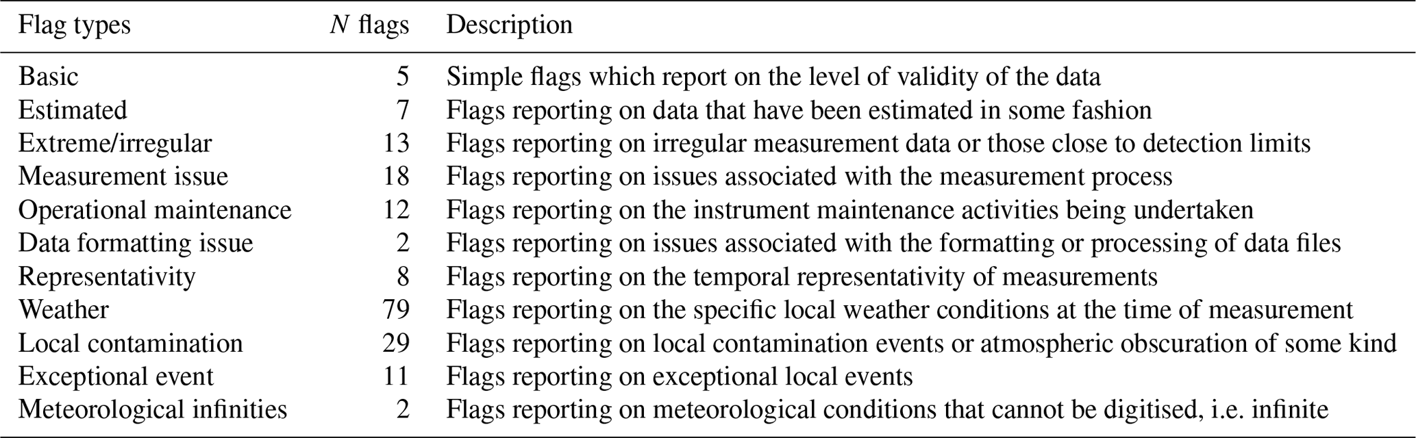
Table 6 Definitions of the simplified standard network QA flags, stored in the flag_simple variable. These flags represent a simplified version of the network QA flags defined in Table A8. These definitions follow those defined in the WaterML2.0 open standards (Taylor et al., 2014).

3.2.5 GHOST quality assurance

Each of the native network QA flags often comes with an associated validity recommendation informing whether a measurement is of sufficient quality to be trusted or not. For example, if the network QA flag is reporting on rainfall at the time of measurement, the recommendation would most probably be that the measurement is valid, whereas, if the flag is reporting on instrumental issues, the recommendation would likely be that the measurement is invalid.

This creates a binary classification where data can be filtered out based on the recommendation of the data provider. This is extremely useful when an end-user simply wants to have data that they know is of a reliable standard and does not wish to preoccupy themselves with choosing which network QA flags to filter by.

As well as writing standard network QA flags per measurement, GHOST's own QA flags are also set, with each flag relating to a GHOST-implemented quality control check. These flags are stored as a list of numerical codes per measurement in the “qa” data variable. A summary table outlining the different GHOST QA flag types is given in Table 10, and the individual standard flag names (and the associated flag codes) are defined in Table A9. Whenever a flag is not active, a fill value (255) is set instead. The majority of these flags are set in Stage 4 of the pipeline (Sect. 3.5). However, a few are set in Stage 1. For example, one of those set is the network recommendation that a measurement should be invalidated: “Invalid Data Provider Flags – Network Decreed” (code 7).

In many instances the network suggestions to invalidate measurements are entirely subjective, and the person who should decide whether a measurement should be retained or not is the end-user themselves. For example, the data provider can recommend that a measurement should be invalidated due to windy conditions, but the end-user may well be interested in such events. We therefore create a GHOST set of binary validity classifications, which are less prohibitive than the original data provider ones. Only in the case that a data flag shows that there has been a technical issue with the measurement or that the measurement has not met internal quality standards is a measurement recommended for invalidation. This is again written as the GHOST QA flag “Invalid Data Provider Flags – GHOST Decreed” (code 6).

Further GHOST QA flags which are set in Stage 1 relate to assumptions or errors found when standardising the metadata associated with measurement processes (described in Sect. 3.2.8) and when an assumption has been made in converting measurement units (described in Sect. 3.2.13).

3.2.6 Metadata

Networks provide metadata in both quantitative and qualitative forms. Metadata are either provided in an external file, stored in the data file header, or given line by line.

Across the networks there is a large variation in the quantity and detail of the metadata reported. In GHOST there is an attempt to ingest and standardise as many available metadata as possible from across the networks, which can be broadly separated into six different types as illustrated in Fig. 2. Table 4 outlines the types of metadata variables standardised in GHOST, and Table A2 defines each of these variables individually.

The standardisation process for the majority of metadata variables consists of mapping the slightly varying variable names, across the networks, to a standard name, e.g. “lat” or “degLat” to “latitude”; converting units (if a numerical variable) to standard ones; and standardising string formatting (if a string variable). For some variables, detailed work is needed to be done to standardise information from across the networks, i.e. station classifications and measurement information, the processes for which are discussed in the subsequent sections. Standardisations are not performed for the descriptive variables (which would be impossible to do) represented in Fig. 2 by the “Further Detail” grouping. If any metadata variable is not provided by a network or the variable value is an empty string, the value in GHOST is set to be NaN.

In GHOST, metadata are treated dynamically. That is, they are allowed to change with time. A limitation of previous data synthesis efforts is that the metadata are static for a station throughout the entire time record. If a station has measured a component from the 1970s to the present day, the typical air sampled at the station could change in a number of ways. For example, a road may be built nearby, the population of the nearest town may swell, or the sampling position may be moved slightly. Significant changes can also occur in the physical measurement of the component. Measurement techniques have evolved over time, and consequently the accuracy and precision of the measurements have improved. All of these factors impact the measurements. Having dynamic metadata allows for inconsistencies or jumps in the measurements over time to be understood, something not possible with static metadata.

The way in which the dynamic metadata are stored in GHOST is in columns. By station, blocks of metadata are associated with a start time, from which they apply. For data files which report metadata line by line, this leads to a vast number of metadata columns, in most cases with no metadata changing between columns. To resolve this duplication, after all metadata parsing and standardisation is complete, each metadata column is cross-compared with the next column, going forwards in time. If all certain key metadata variables in the next column are identical to the current column, the next column is removed entirely. These key variables are defined by metadata group type in Table A12.

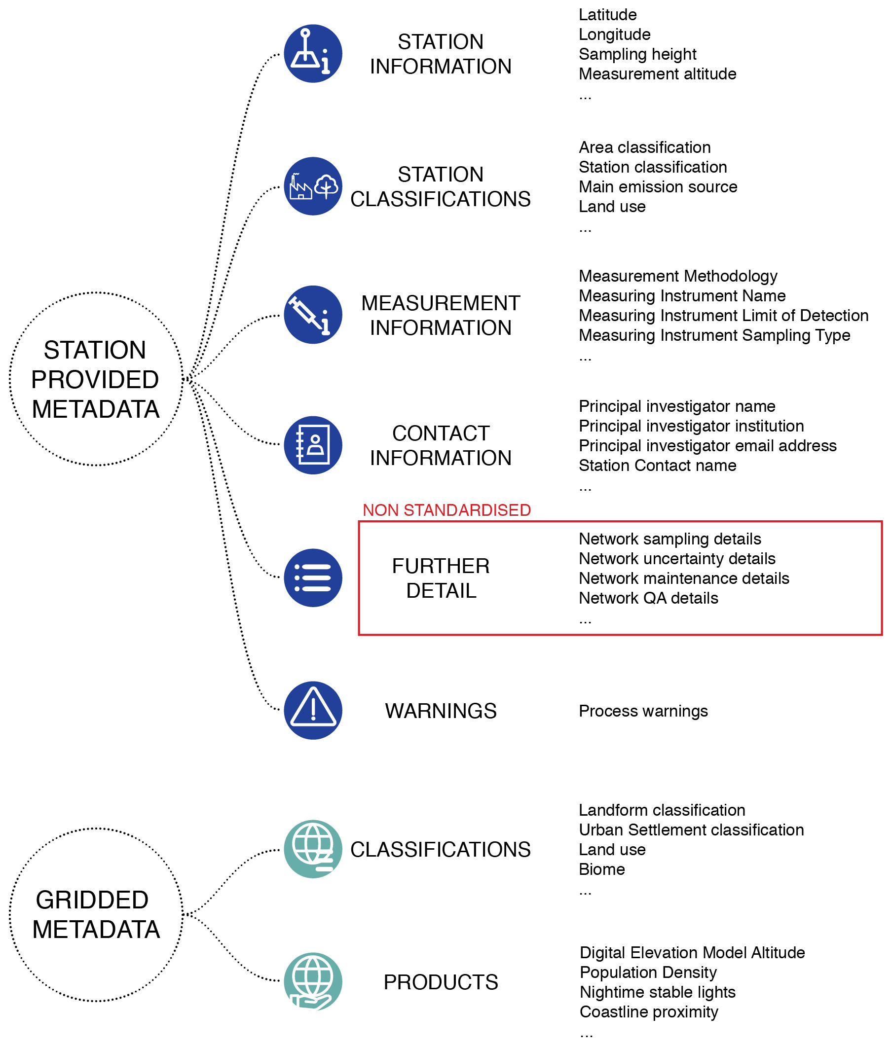
Figure 2 Visual summary of the types of metadata ingested and standardised in GHOST. The metadata can be separated into two distinct categories, station-provided metadata and gridded metadata.

3.2.7 External metadata join

When metadata are reported in external file(s) separate from the data, they are typically associated with the data using the network station reference. In some cases, the association is made using a sample ID, with individual measurements tagged with an ID that is associated with a specific collection of metadata. Stations with which external metadata cannot be associated and where there is no other source of metadata (i.e. in the data files) are excluded from further processing.

The metadata values in the external files are assumed to be valid across the entire time record. For the specific case of Japan NIES, external metadata files are provided per year, permitting updates to the metadata with time.

For some networks there are several different external metadata files provided, e.g. EEA AQ e-Reporting. Some of the metadata variables across these files are repeated, whereas some are unique to specific files. To solve this, the external files are given priority rankings, so that when variables are repeated, it is known which file to preferentially take information from.

For some networks, no metadata are provided, either in the data files or in external files, and therefore the metadata for key variables (e.g. longitude, latitude, or station classification) are compiled manually in external files. This is done principally using information gathered from network reports or documentation. For other networks, the provided metadata are very inconsistent from station to station, and therefore external metadata files are compiled manually to ensure that some key variables are available across all stations, e.g. station classifications. Manually compiled metadata are only ever accepted for a variable when there are no other network-provided metadata for that variable available throughout the time record.

When station classifications are compiled manually, this is first attempted by following network documentation on how exactly the classifications are defined. If no documentation exists, this is then done by assessing the available network station classifications in conjunction with their geographical position using Google Earth to attempt to empirically understand the classification procedures. The stations are then classified following this empirically obtained logic.

3.2.8 Measurement process standardisation

The type of measurement processes implemented in measuring a component can have a huge bearing on the accuracy of measurements. Despite most networks providing information which details some aspects of the measurement processes, this information is incredibly varied in terms of both detail and format.

Within GHOST, substantial efforts are made to fully harmonise all information relating to the measurement of a component. As there are 227 components processed within GHOST, there is naturally a huge number of differing processes used to measure all of these different components. For example, for O₃, as it is relatively easy to measure, a stand-alone instrument both samples and measures the concentration continuously. For speciated PM₁₀ measurements, a filtering process is first needed to separate the PM by size fraction, and then a speciated measurement of the relevant size fraction is performed.

In GHOST, an attempt is made to standardise all measurement processes across three distinct measurement steps: sampling, sample preparation, and measurement. The “sampling” step refers to the type of sampling used to gather the sample to be measured, “sample preparation” refers to processes used to prepare the sample for measurement, and “measurement” refers to the ultimate measurement of the sample.

Combining information across these three different steps can be used to subsequently describe all different types of measurement processes. Figure 3 visually shows some typical measurement configurations that can be described by mixing these steps. For example, the measurement of O₃ is represented by the “automatic” configuration, where information from the sampling and measurement steps is sufficient to describe the measurement process. That is, there is no preparation step.

In GHOST, a database has been created that identifies and stores information from across the measurement steps in a standardised format. For the sampling step, eight different sampling types and 83 different instruments which employ the sampling types are identified and defined in Table A5. For the sample preparation step, 10 different preparation types and 20 specific techniques which employ the preparation types are identified and defined in Table A6. For the measurement step, 104 different measurement methods and 508 different instruments which employ the methods are identified and defined in Table A7.

For each specific sampling or measuring instrument, there is typically documentation published outlining the relevant specifications of the instrument, e.g. providing information about the limits of detection and the flow rate. Where this documentation is made available online, it is downloaded and parsed, and the relevant specifications are associated with the standard instruments in the database.

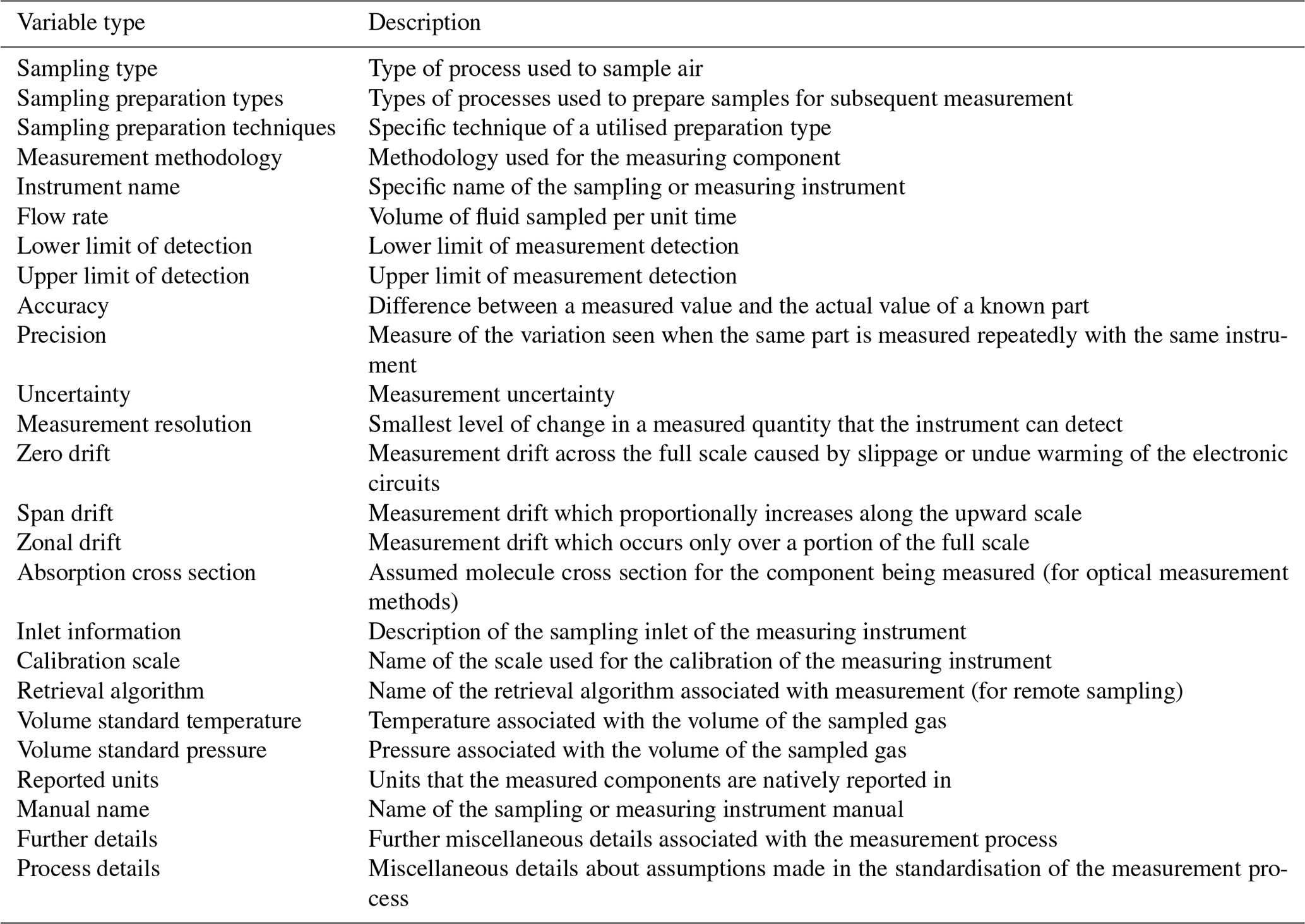
In order to connect network-reported metadata with the standard information in the database, firstly, all network-provided metadata associated with measurement processes are gathered and concatenated into one string. These strings are then manually mapped to standard elements in the database. This mapping procedure is a huge undertaking but ultimately returns a vast quantity of standardised specification information that can be associated with measurements. Table 7 outlines all the types of measurement metadata variables that information is returned for, with the full list of available variables given in Table A2 in the “Measurement information” section. All the measurements are therefore associated with a standard measurement method, the abbreviation for which (defined in Table A7) forms the second part of the station_reference variable defined in Sect. 3.2.1. In some cases, the networks themselves provide some measurement specification information. This can differ in some cases from the documented instrument specifications, as there may be station-made modifications to the instrumentation, thereby improving upon the documented specifications. This reported information is also ingested in GHOST for the exact same specification variables as ingested in the documented case. There are therefore two variants for each of these variables. All variables which contain the “reported” string contain information from the network, whereas variables containing the “documented” string contain information from the instrument documentation.

Multiple QA checks are also performed throughout the standardisation process. Each standardised sampling type or instrument, sample preparation type or technique, and measurement method or instrument is associated with a list of components for which they are known to be associated with (1) the measurement and (2) the accurate measurement.

For example, for the first point, the “gravimetry” measurement method is not associated with the measurement of O₃. Therefore, this method would be identified as erroneous and the associated measurements flagged by GHOST QA (“Erroneous Measurement Methodology”, code 22 in this case). For the second point, the “chemiluminescence (internal molybdenum converter)” method is associated with the measurement of NO₂, but there are known major measurement biases (Winer et al., 1974; Steinbacher et al., 2007). Therefore, these instances would also be flagged by GHOST QA (“Invalid QA Measurement Methodology”, code 23).

Table A7 details the components whose measurements each standard measurement method is known to be associated with, together with the components that each method can accurately measure. Additional GHOST QA flags are set when the specific names of the types, techniques, methods, and instruments are unknown as well as when any assumptions have been made in the mapping process. All of these flags are defined in Table A9 in the “Measurement process flags” section.

Figure 3 Visual illustration of the three GHOST standard measurement process steps and how these steps are combined in the most typical measurement configurations. The three standard steps are sampling, preparation, and measurement.

Table 7 Outline of the types of standard metadata variables in GHOST associated with the measurement process. A description is given for each variable. Many of these variable types will have two associated variables, one giving network-reported information and the other giving information stemming from instrument documentation. More information is available in Table A2.

3.2.9 Measurement limits of detection and uncertainty

In some cases, measurements will be associated with estimations of uncertainty and limits of detection (LODs), both lower and upper, by the measuring network. These can be provided per measurement or as constant metadata values. This information is incredibly useful scientifically, as it allows for the screening of unreliable measurements.

In GHOST this information is captured as GHOST QA flags whenever LODs are exceeded, “Below Reported Lower Limit of Detection” (code 71) and “Above Reported Upper Limit of Detection” (code 74), and as a data variable for the measurement uncertainty, “reported_uncertainty_per_measurement”.

This information can be complemented by documented information associated with the measuring instrument (if known). If documented LODs for an instrument are exceeded, this sets the GHOST QA flags “Below Documented Lower Limit of Detection” (code 70) and “Above Documented Upper Limit of Detection” (code 73). Typically, the reported network information is to be preferred over the documented instrument information, as any manner of modifications may have been made to the instrument post sale. Two GHOST QA flags encapsulate this concept neatly, first trying to evaluate LOD exceedances using the reported information if available and, if not, then using the documented instrument information: “Below Preferential Lower Limit of Detection” (code 72) and “Above Preferential Upper Limit of Detection” (code 75).

In some cases the measurement uncertainty is not provided directly but can be calculated from other associated metadata information (network-reported information again being preferred to instrument documentation). This is done using the quadratic addition of measurement accuracy and precision metrics and is saved as the data variable “derived_uncertainty_per_measurement”.

All of this information is converted to the standard units of the relevant component (see Sect. 3.2.13) before setting QA flags or metadata and data variables.

3.2.10 Station classification standardisation

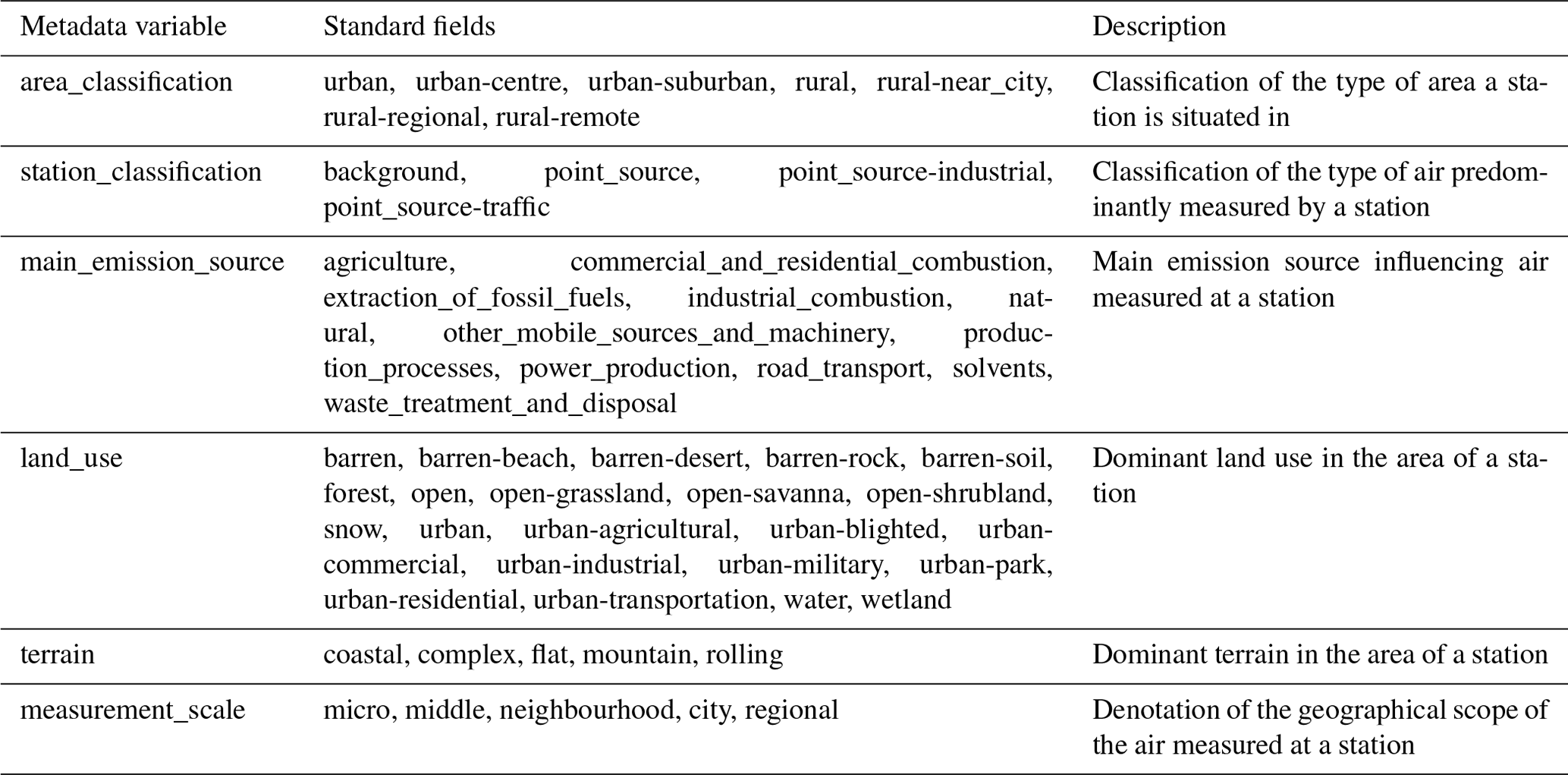
The networks provide a variety of station classification information, which can be used to inform the typical types of air parcels seen at a station. Within GHOST, all this classification information is standardised to six metadata variables, as outlined in Table 8.

For each standard classification variable, the available class fields are also standardised, which is done through an extensive assessment of all available fields across the networks. This process is inherently associated with some small inconsistencies, as there is not always a perfect alignment between the available class fields across the networks or significant variation in the granularity of fields in some cases, e.g. for station area classifications “urban” and “urban centre”. In order to account for variations in field granularity, all standard class fields can consist of a primary class and sub-class separated by “-”, e.g. “urban” or “urban-centre”. These fields are defined per variable in Table A4.

Table 8 Outline of the GHOST standard station classification metadata variables, the standard fields per variable, and a description of each variable. In Table A4, each of the fields per variable is defined.

3.2.11 Check the measurement position's validity

After all metadata information has been parsed, some checks are done to ensure that the measurement position metadata are sensible in nature, with the checks done as follows:

1. Check whether the longitude and latitude are outside valid bounds, i.e. outside the −180° ↔ 180° and −90° ↔ 90° bounds respectively.

2. Check whether the longitude and latitude are both equal to 0.0, i.e. the middle of the ocean. In this case the position is assumed to be erroneous.

3. Check whether the altitude and measurement altitude are less than −413 m, i.e. lower than the lowest exposed land on Earth, the Dead Sea shore.

4. Check whether the sampling height is less than −50 m. Such a sampling height being so far below the station altitude would be extremely strange.

Any measurement position metadata failing any of the these checks are set to be NaN. Any stations associated with longitudes or latitudes equal to NaN are excluded from further processing.

3.2.12 Correcting duplicate or overlapping data

Some network data files contain duplicated or overlapping measurement windows. Work is done to correct these instances and ensure that measurements and all other data variables (e.g. qa or flag) are placed in ascending order across time.

Measurement start times are first sorted in ascending order. If any measurement windows are identically duplicated, i.e. have the same start and end times, the windows are iteratively screened by the GHOST QA flags “Not Maximum Data Quality Level” (code 4), “Preliminary Data” (code 5), and “Invalid Data Provider Flags – GHOST Decreed” (code 6), in that order, until the duplication is resolved. If there is still a duplication after screening, the first indexed measurement window is kept preferentially and the others dropped.

After removing the duplicate windows, we next check whether any measurement window end times overlap with the next window's start time. If an overlap is found, the windows are again screened iteratively by GHOST QA flags 4, 5, and 6, in that order, until the duplication is resolved. If there is still an overlap, the remaining windows with the finest temporal resolution are kept. For example, hourly resolution is preferred to daily. If this still does not resolve the overlap, the first indexed remaining measurement window is kept preferentially.

Both of these processes are done recursively until each measurement window does not overlap with any other and has no duplicates.

3.2.13 Measurement unit conversion

A major challenge in a harmonisation effort such as GHOST is that components are often reported in various different units and in many instances report entirely different physical quantities that require complex conversions.

In GHOST, each component is assigned the standard units listed in Table A3 to which all natively provided units are converted. The units for all components in the gas and particulate (PM, PM₁₀, PM_2.5, and PM₁) matrices are reported as either mole fractions (e.g. ppbv = nmol mol${}^{-\mathrm{1}}=\mathrm{1}\times {\mathrm{10}}^{-\mathrm{9}}$ mol mol⁻¹) or mass densities (e.g. µg m⁻³) in a range of different forms across the networks. All gas components are standardised to be mole fractions, whereas all particulate components are standardised to be mass densities. Components in the other matrices are all unitless, except for vconc and size, which are standardised (µm³ µm⁻²). Components for these two matrices all stem from the AErosol RObotic NETwork (AERONET) v3 Level-1.5 and AERONET v3 Level-2.0 networks and are already reported in GHOST standard units. Unit conversion is therefore only handled for gas and particulate matrix components.

Almost all gas and particulate measurement methodologies fundamentally measure in units of number density (e.g. molec. cm⁻³) or as a mass density, not as a mole fraction. The conversion from a number density to a mass density is simply

$$\begin{array}{}\text{(1)}& {\mathit{\rho }}_{\mathrm{C}}={\displaystyle \frac{{\mathit{\rho }}_{N\mathrm{C}}\cdot M_{\mathrm{C}}}{N_{\mathrm{A}}}},\end{array}$$

where ρ_C is the mass density of the component (g m⁻³), ρ_NC is the number density of the component (molec. m⁻³), M_C is the molar mass of the component (g mol⁻¹), and N_A is Avogadro's number (6.0221×10²³ mol⁻¹).

The conversion from mass density to mole fraction depends on both temperature and pressure:

$$\begin{array}{}\text{(2)}& V_{\mathrm{C}}={\mathit{\rho }}_{\mathrm{C}}\cdot {\displaystyle \frac{RT}{M_{\mathrm{C}}P}},\end{array}$$

where V_C refers to the component mole fraction (mol mol⁻¹), R is the gas constant (8.3145 J mol⁻¹ K⁻¹), P is pressure (Pa), and T is temperature (K). The temperature and pressure variables refer to the internal temperature and pressure of the measuring instrument, not the ambient conditions, physically relating to the volume of the air sampled.

Some component measurements are reported in units of mole fractions per element, e.g. ppbv per carbon or ppbv per sulfur. These units are converted to the mole fractions of the entire components by

$$\begin{array}{}\text{(3)}& V_{\mathrm{C}}={\displaystyle \frac{V_{\mathrm{C}}}{A_{\mathrm{EC}}}},\end{array}$$

where V_EC is the mole fraction per element (mol mol⁻¹) and A_EC is the number of relevant element atoms in the measured component (e.g. two carbon atoms in C₂H₄).

In a small number of instances, measurements of total VOCs (volatile organic compounds), total NMVOCs (non-methane volatile organic compounds), total HCs (hydrocarbons), and total NMHCs (non-methane hydrocarbons) are reported as mole fractions per carbon. As these measurements sum over various components, there is no fixed number of carbon atoms. It is assumed that these measurements are normalised to CH₄, i.e. one carbon atom, as is done typically.

In order to ensure that measurements are comparable across all stations, they are typically standardised by each network to a fixed temperature and pressure, i.e. no longer relating to the actual sampled gas volume. The standardisation applied differs by network but in almost all cases also follows EU or US standards. The EU standard sets the temperature and pressure as 293 K and 1013 hPa (European Parliament, 2008), whereas the US standard is 298.15 K and 1013.25 hPa (US EPA, 2023). The differently applied standards can lead to significant differences in the reported values of the same initial measurements. For example, a CO measurement of 200 µg m⁻³, with an internal instrument temperature and pressure of 301.15 K and 1000 hPa, is 3.55 µg m⁻³ higher following EU standards compared to US ones (208.2 vs. 204.7 µg m⁻³). This means that the same measurements using EU standards will always be slightly higher (1.7 %) than those using US standards.

To attempt to remove this small inconsistency across the networks, after measurement unit conversion, all gas and particulate matrix measurements are re-standardised to the GHOST-defined standard temperature and pressure of 293.15 K and 1013.25 hPa, which is equivalent to the normal temperature and pressure (NTP). An assumption is made that the original units of measurement are either a mass or a number density, i.e. that the measurement is dependent on temperature and pressure.

This standardisation is only done when there is confidence in the sample gas volume associated with measurements. That is, the volume standard temperature and pressure are reported, or there is a known network standard temperature and pressure for a component. When any assumptions are made when performing this standardisation or the sample gas volume is unknown, GHOST QA flags are written that are outlined in the “Sample gas volume flags” section in Table A9.

The standard unit is mass density, and the standardisation is done by

$$\begin{array}{}\text{(4)}& S_{\mathrm{C}}={\mathit{\rho }}_{\mathrm{C}}\cdot {\displaystyle \frac{T_N}{\mathrm{293.15}}}\cdot {\displaystyle \frac{\mathrm{1013.25}}{P_N}}.\end{array}$$

When the standard units are a mole fraction, the conversion is done by

$$\begin{array}{}\text{(5)}& S_{\mathrm{C}}=M{R}_{\mathrm{C}}\cdot {\displaystyle \frac{\mathrm{293.15}}{T_N}}\cdot {\displaystyle \frac{P_N}{\mathrm{1013.25}}},\end{array}$$

where S_C is the GHOST standardised value, T_N is the known standard temperature, and P_N is the known standard pressure.

3.3 Concatenate parsed station data files (Stage 2)

Now that all data files for a network and component pair have been parsed and saved in standardised equivalent files, the next step is to concatenate all files associated with the same station, creating a complete time series.

Typically this is a very easy process simply joining the files together through the time record. However, it quickly becomes very complex when there are duplicated or overlapping files. Choosing which file to take data from each file conflict is a tricky issue, for which a number of factors need to be taken into consideration.

In Stage 2 of the pipeline, a methodology is implemented to systematically resolve each of these file conflicts by station. Additional work is done to fill gaps in the metadata across the time record, and finally a check is undertaken to determine whether the station measurement position is consistent across the time record. Where there are significant changes in the measurement position, station data are split apart to reflect the significantly different air masses being measured. Figure 4 visually describes the Stage-2 operation.

Parallelisation is done by unique station (via station_reference) in the stage.

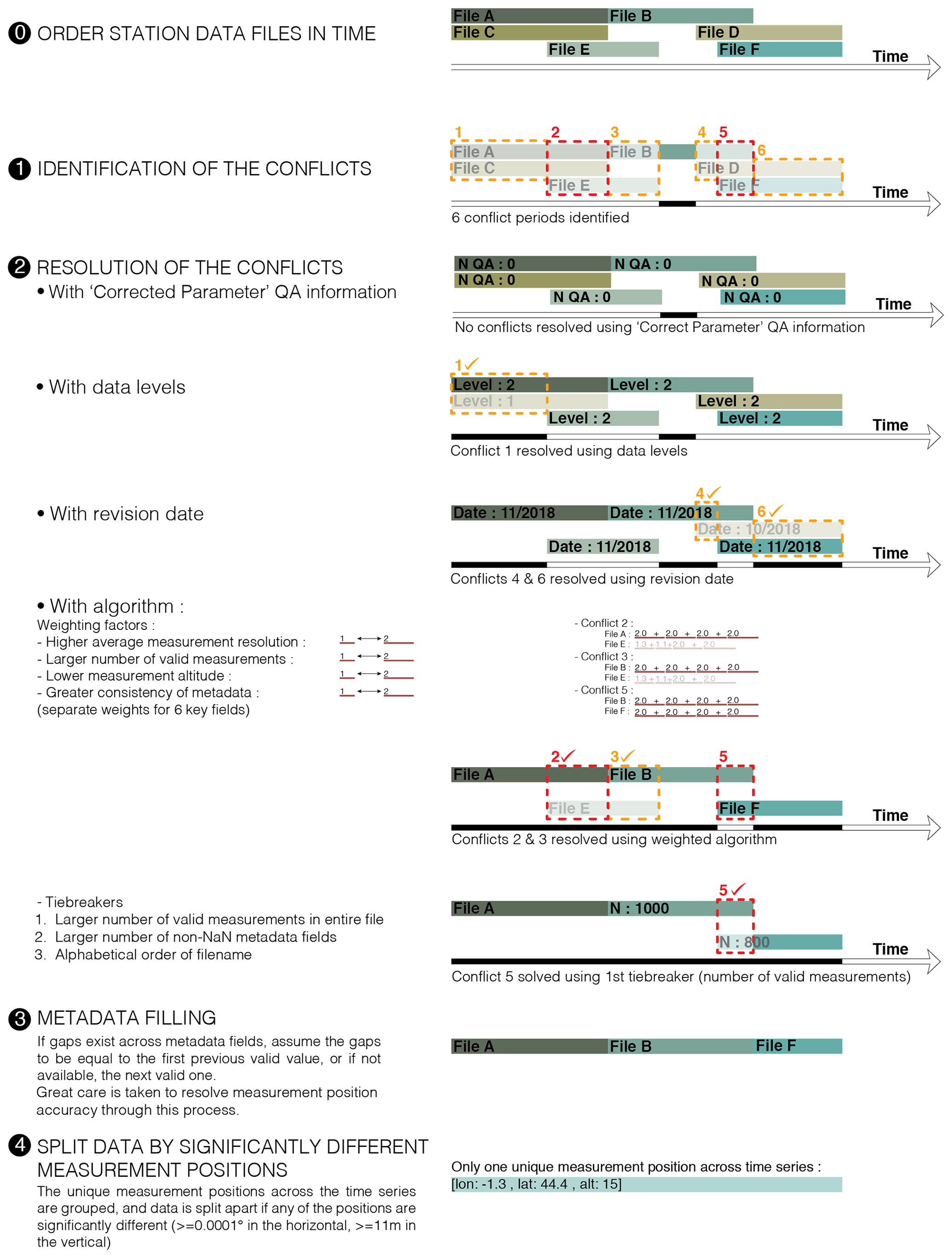
Figure 4 Visual illustration of the resolution process for temporally conflicting parsed station data files, in Stage 2 of the GHOST pipeline, when concatenating station data across time.

3.3.1 Data join

For each unique station (via station_reference), all associated Stage-1-written files are gathered and read into memory.

An assessment is first made of whether there are any data overlaps between any of the files through the time record. If no overlaps are found, the data or metadata in the files are simply joined together. If any overlaps are found, the relevant periods and files are logged and a stepped process is undertaken to determine which file should be retained in each overlap instance:

• 1.

  First, we attempt to resolve the overlap using the number of measurements associated with the GHOST QA flag “Corrected Parameter” (code 24). This flag applies to measurements for which there is typically a known issue with the measurement methodology and some type of correction has been applied to improve the accuracy of the measurement. The maximum number of measurements associated with the QA flag are taken across the conflicting files, and only files equal to the maximum number of associated measurements are kept.

• 2.

  Second, priority data levels are used. Networks often publish the same data files multiple times with continuously improved QA, e.g. near real time, then with automatic QA, and finally with manual QA validation. Each type of data release is associated with a defined data level (stored in the data_level metadata variable) and are all given a hierarchical priority ranking. For example, EEA provides data in two separate streams: E1a (validated) and E2a (near real time). E1a is preferred to E2a in this case. The maximum ranking across the conflicting files is taken, and only files with that ranking are retained.

• 3.

  Third, the data revision date is used. Data files are often published with the same data level but different data revision dates, with files often needing to be republished after processing errors are identified and corrected. The data revision date is used to differentiate between these files. The latest revision date across the conflicting files is taken, and only files with that revision date are retained.

• 4.

  Fourth, a ranking algorithm is used. For each file, a number of weighting factors contribute normalised ranking scores between 1 and 2, which are then summed to give the total ranking score. The file with the highest score is then selected. The weighting factors considered in the ranking algorithm are as follows:

  • –

    Average temporal resolution in the overlap period: a finer temporal resolution (i.e. a smaller number) gives a higher weighting.

  • –

    Number of valid measurement points in the overlap period (after screening by the GHOST QA flag “Invalid Data Provider Flags – GHOST Decreed”, code 6): a higher number gives a higher weighting.

  • –

    Measurement altitude: this is designed to deal with instances where measurements are made on towers, simultaneously measuring components at different altitude levels. Lower measurement altitudes are given a higher weighting.

  • –

    Consistency of metadata in the overlapping files with those across all other files across the entire time record: a weighted score is calculated for each of the longitude, latitude, altitude, measurement altitude, measurement methodology, and measuring instrument name variables. Files with values which occur more frequently over the time record are given a higher weighting.

    After this, only files with summed rankings equal to the maximum score are retained.

• 5.

  Finally, if there are still two or more remaining files for an overlap instance, some tiebreak criteria are used to select a file:

  • –

    first, by the maximum number of valid measurement points across the whole data files, i.e. not just the valid values for the overlap period (after screening by the GHOST QA flag “Invalid Data Provider Flags – GHOST Decreed”, code 6);

  • –

    second, by the maximum number of non-NaN metadata variables provided in each data file; and

  • –

    finally, if there is still a tie after sorting the filenames alphabetically, the first file is chosen.

After selecting a file in each overlapping period, the data and metadata in the files are simply joined together across the time record.

3.3.2 Resolve the measurement position accuracy

After joining the data files, a consistent time series now exists for each station. However, some irregularities may exist in the stored metadata through the time record. This is of specific concern for the variables associated with the measurement position, i.e. longitude, latitude, altitude, sampling height, and measurement altitude.

In some instances, the level of accuracy of the network-provided measurement position metadata varies over time. This can cause significant ramifications, with the difference of a decimal place or two being able to significantly shift the subsequent evaluation of station data, e.g. placing a station incorrectly over the sea or in an erroneous valley or peak in mountainous terrain. Most of these instances are simply explained by errors in the creation of the data files or the number of reported decimal places changing over time.

To attempt to rectify the majority of these cases, a two-step procedure is undertaken:

1. First, for each measurement position variable, all non-NaN values across the time record are grouped together within a certain tolerance (0.0001° $=\sim \mathrm{11}$ m for longitude and latitude, 11 m for altitude, sampling height, and measurement altitude). Values that are within the tolerance of at least one other position would all be grouped together, e.g. [10 m, 17 m, 21 m]. However, without the 17 m value, [10 m] and [21 m] would be in separate groups. The weighted modal measurement position in each group is then determined using the number of sampled minutes that each metadata value represents as weights, and the value of this position is then used to overwrite the original measurement position values in the group through the time record.

2. Second, for each variable, all values which are sub-strings of any of the other positions across the time record are grouped together. For example, 0.01 is a sub-string of 0.012322. In each group, an assumption is made that each sub-string is actually referring to the most detailed version of the position in the group, i.e. that with the most decimal places. If there are two or more positions with the same maximum level of decimal places, the position which represents the greater number of sampled minutes is chosen. This chosen position is then used to overwrite the original measurement position values in the group through the time record.

In both steps, information is written to the process_warnings metadata variable, informing of the assumptions made in these procedures.

3.3.3 Handle gapped key metadata

Generally speaking, the level of detail in the reporting of metadata has improved over time. This means in many cases that metadata variables that were not reported in the past are now. In some instances, a metadata variable is inexplicably not included in a file when it was previously or subsequently reported, in most cases presumably due to a formatting error. As metadata are handled dynamically in GHOST, both circumstances lead to gaps in the metadata variables throughout the time record.

In most cases the provided metadata are constant over large swathes of time; therefore, taking metadata reported previously or subsequently in the time record can be justifiably assumed to be applicable for the missing periods. We thus attempt to fill the missing metadata for each variable. This is done by taking the closest non-NaN value going backwards in time for each variable or, if none exists, the closest non-NaN value going forwards in time. For positional metadata this stops stations from being separated out due to small inconsistencies through the time record (Sect. 3.3.5).

Some dependencies are required for this filling procedure for some metadata variables to prevent incompatibilities in concurrent metadata variables. For example, the documented lower limit of detection of a measuring instrument should not change if the measuring instrument does not. These dependencies are defined in Table A13. Because of the importance of positional variables being set (e.g. latitude), filling is attempted through several passes, using progressively less stringent dependencies before ultimately requiring zero dependencies. The filling is not performed for any metadata variables that are highly sensitive with time (these being the non-filled group in Table A13). If data are filled for any key variables, which are defined in Table A12), a warning is written to the “process_warnings” variable.

3.3.4 Set altitude variables

The three GHOST measurement position altitude variables are all interconnected in that altitude + sampling height = measurement altitude. A series of checks is performed to ensure that this information is consistent through the time record and modified if not. For any variables that are modified, information is written to the process_warnings variable. Per metadata column, the checks proceed as follows:

1. If all three altitude variables are set, i.e. non-NaN, we check whether all the variables sum correctly. If not, the measurement altitude variable is recalculated as altitude + sampling height.

2. If only two variables are set, the non-set variable is calculated from the others, e.g. altitude =10 m and sampling height =2 m, and therefore measurement altitude is calculated to be 12 m.

3. If only one variable is set and it is the altitude or measurement altitude, the other altitude variable is set to be equivalent, i.e. altitude = measurement altitude, and the sampling height is set to 0.

4. If no altitude or measurement altitude is set, it is subsequently set using information from a digital elevation model (DEM) detailed in Sect. 3.4.6.

3.3.5 Split stations by significantly changing measurement position

The final check in Stage 2 determines whether the measurement position of a station changes significantly through the time record, i.e. whether one of the longitude, latitude, or measurement altitude changes. Where there are significant changes, the associated data or metadata are separated out over the time record. Each separate grouping is then considered a new station, reflecting the fact that the air masses measured across the changing measurement positions may be significantly different.

The unique measurement positions across the time record are firstly grouped within a certain tolerance (0.0001° $=\sim \mathrm{11}$ m for longitude and latitude and 11 m for the measurement altitude), as in Sect. 3.3.2. Grouping like this ensures that, if the measurement position changes and then later reverts to the previous position, the associated data for the matching positions would be joined.

After the grouping process, some checks are performed to ensure that each of the groupings is of a sufficient quality to continue in the GHOST pipeline:

1. If there are more than five unique groupings found, the station is excluded from further processing as the associated data are not considered to be trustworthy.

2. If any grouping has <31 d of the total data extent, this group is dropped from further processing, as it is not considered of sufficient relevance to continue processing.

3. For each grouping, if there are too many associated metadata columns per total data extent (≤90 d per column), the group is dropped from further processing, as the metadata are considered too variable to be trusted.

After these checks, if there is more than one remaining measurement position grouping, the associated data or metadata are split, all associated with a new station_reference. The data which have the oldest associated time data retain the original station_reference. Each chronologically ordered grouping after that is associated with a new station_reference defined as “[station_reference]_S[N]”, where N is an ascending integer starting from 1.

3.4 Add gridded metadata (Stage 3)

At this point in the pipeline, all station data and metadata for a component reported by a given network have been parsed, standardised, and concatenated, creating a complete time series for each station. In the next three stages (3–5), the processed network data are complemented through the addition of external information by station, giving added value to the dataset.

In many cases where observational data are used by researchers, they are used in conjunction with additional gridded metadata. This typically represents objective classifications or measurements of some kind made over large spatial scales, i.e. typically continental to global. In some previous data synthesis efforts, some of the most frequently used gridded metadata in the atmospheric composition community were ingested and associated by station.

GHOST follows this example, specifically looking to build upon the collection of metadata ingested by Schultz et al. (2017). A distinction was made between the types of gridded metadata ingested, i.e. “Classification” and “Product”, as outlined in Fig. 2. “Product” metadata are numerical in nature, whereas “Classification” metadata are not.

One key example of the added value of these gridded metadata is when looking to filter out high-altitude stations. When surface observations are used for model evaluation, it is typically desirable to remove stations in hilly or mountainous regions, as the models typically do not have the horizontal resolution to correctly capture the meteorological and chemical processes in these regions. The exclusion of stations is typically done by filtering out all stations above a certain altitude threshold, e.g. 1500 m from the mean sea level. This is a very simplistic approach, as it does not take into account the actual terrain at the stations and means that low-altitude stations which lie on very steep terrain are not removed, and high-altitude stations which lie on flat plateaus are filtered out (e.g. much of the western US). A better approach would be to filter stations by the local terrain type. There exist numerous sources of gridded metadata which globally classify the types of terrain, the two of them ingested by GHOST being the Meybeck (Meybeck et al., 2001) and Iwahashi (Iwahashi and Pike, 2007) classifications. Figure 5 shows these two classification types in comparison with gridded altitudes from the ETOPO1 DEM. In areas such as southern and central Europe, the two terrain classifications indicate that there is lots of very steep land, whereas the DEM indicates that the majority of the land lies at relatively low altitudes (<500 m).

Table 9 shows a summary of the gridded metadata ingested in GHOST, with the associated temporal extents and native horizontal resolutions by metadata variable. Table A11 provides more information about the ingested metadata, specifically the spatial extents, projections, horizontal or vertical data, and native file formats. All of the gridded metadata that are ingested in GHOST provide information on a global scale in longitudinal terms, but some do not provide full coverage of the poles, e.g. the ASTER v3 altitude of −83 to 83° N.

The major processes involved in the association of gridded metadata in GHOST are described in the following sub-sections. As well as ingesting and associating gridded metadata by station, other globally standard metadata variables are also associated by station, i.e. reverse geocoded information and local time zones as described in Sect. 3.4.4 and 3.4.5.

Parallelisation is done by unique station (via station_reference) in the stage.

Figure 5 Comparison of the variety of gridded metadata available for the classification of terrain ingested in GHOST. Shown are two landform classifications, Meybeck and Iwahashi, as well as the ETOPO1 DEM altitude.

(NASA et al., 2018)(NOAA NGDC, 2009)(Crippa et al., 2018; EC JRC and Netherlands PBL, 2017)(Iwahashi and Pike, 2007; ESDAC, 2024)(Meybeck et al., 2001; ESDAC, 2024)(CIESIN and CIAT, 2005)(CIESIN, 2018)(Corbane et al., 2018, 2019)(Freire et al., 2016; Schiavina et al., 2019)(Ehrlich et al., 2019; Pesaresi et al., 2019)(NASA OBPG, 2024)(Beck et al., 2018)(Friedl and Sulla-Menashe, 2015)(Friedl and Sulla-Menashe, 2015)(Friedl and Sulla-Menashe, 2015)(NOAA and US Air Force Weather Agency, 2024)(Krotkov et al., 2017, 2019)(Krotkov et al., 2017, 2019)(Krotkov et al., 2017, 2019)(Krotkov et al., 2017, 2019)(WMO, 2024a)(Olson et al., 2001)(Olson et al., 2001)(Olson et al., 2001)(Ellis et al., 2010; University of Maryland Baltimore County, 2024)

Table 9 Summary of the gridded metadata which are ingested in GHOST. The temporal extent of each metadata type is given, together with the native horizontal resolution of each type. More information is given in Table A11.

3.4.1 Dynamic gridded metadata

For most of the gridded metadata types ingested in GHOST, the provided metadata are representative of an annual period, which is updated annually.

As with the network-provided metadata, there is a conscious effort to capture the changes in the ingested gridded metadata across time. This is of specific importance for products directly affected by anthropogenic processes, e.g. land use or population density. However, processing gridded metadata for every year, in theory from 1970 to 2023, would place a major strain on the processing workflow, and therefore a compromise is needed. For each different gridded metadata type, the first and last available metadata years are ingested, together with updates within this range in years coinciding with the start and middle years of each decade, e.g. 2010 or 2015. The specific ingested temporal extents for each type of gridded metadata are defined in Table 9. Each metadata column is matched by station with the most temporally consistent gridded metadata through the minimisation of the metadata column centre time and the gridded metadata centre extent time.

3.4.2 The 5 and 25 km modal and average gridded metadata

The parsing and association of the gridded metadata by station are in most cases done by taking the value of the grid cell in which the longitude and latitude coordinates of the station lie (i.e. nearest-neighbour interpolation). Some gridded metadata are provided in non-uniform polygons, i.e. Shapefile and GeoJSON formats, adding additional complexity.

The extremely fine horizontal resolution of some of the ingested gridded metadata, e.g. 250 m, means that they may often be incomparable with data sources at coarser resolutions, e.g. data from a global CTM. To help in situations such as this, for each ingested gridded metadata variable of a fine enough horizontal resolution, extra variables are written taking the average or mode in 5 and 25 km radii around the station coordinates. The mode is taken for “Classification” variables, and the average is taken for “Product” variables. No additional variables are created for gridded metadata, which are natively provided in Shapefile and GeoJSON formats.

In order to calculate which grid boxes are taken into consideration in the modal or average calculations, perimeters 5 and 25 km around the longitude and latitude coordinates are calculated geodesically following Karney (2013). The percentage intersection of each grid cell with the perimeters is then calculated. That is, how much of each grid cell is contained within the perimeter bounds?

When calculating the modal Classification variables, the class values are simply set as the class which appears most often over all grid cells with an intersection greater than 0.0. When calculating the average Product variables, the weighted average is taken across all grid cells with an intersection greater than 0.0, using the percentage intersections as weights.

3.4.3 Coastal correction

Due to the nature of grids, stations which are located very close to the coast could occasionally could fall into grid cells which are predominantly situated over water and are thus associated with metadata which are not representative of the station. For the regularly gridded Classification variables, a correction for this is attempted.

In all cases where the metadata class is initially determined to be “Water”, the modal class across the primary grid cell and its surrounding grid cells (i.e. sharing a boundary, including diagonally) is calculated, overwriting the initially determined class. If the primary grid cell is far from the coast, the class will be maintained as Water, but if it is close to the coast, the set class will more likely be representative of the coastal station.

3.4.4 Reverse geocoded station information

Reverse geocoding is the process of using geographical coordinates to obtain address metadata. The Python reverse_geocoder package (Thampi, 2024) provides a library which provides this function. Specifically, for each provided longitude and latitude coordinate pair, metadata are returned for the following variables: “city”, “administrative_country_division_1”, “administrative_country_division_2”, and “country”. This is extremely useful, as it allows station address metadata to be standardised across the networks.

In some cases, when stations are extremely remote, the returned search information is matched to a location extremely far from the original coordinates. To guard against such instances, the matched location is required to be within a tolerance of 5° of the station longitude and latitude.

3.4.5 Local time zone

As well as using the station coordinates to obtain standard address metadata, they can be used to obtain the local time zone. This is done by passing a station longitude–latitude coordinate pair to the Python timezonefinder package (Michelfeit, 2024). This returns a local time zone string, referencing the IANA time zone database (IANA, 2024), which is saved to the station_timezone metadata variable.

In some cases, if the station is extremely remote, the timezonefinder package will not be able to identify a local time zone. In these cases, the closest time zone is identified within a set radius around the station of initially 1°. If no time zones are identified within this initial radius, the radius size is increased iteratively by 1° until a time zone is found. This iteration is allowed to continue for 1 min before timing out, and the station time zone is left unset.

If the timezonefinder package is used to obtain the local time zone in order to shift local time measurements to UTC (see Sect. 3.2.3), this of course carries some uncertainty, and thus any measurements shifted in such a fashion are accompanied by the GHOST QA flag “Timezone Doubt” (code 61).

3.4.6 Set missing altitude metadata using a DEM

As referenced in Sect. 3.3.4, if no altitude or measurement altitude is set through the time record for a station, it is set using information from a DEM.

This is first done by taking altitudes from the ASTER v3 DEM (NASA et al., 2018). Missing altitude variable metadata (i.e. NaN) are simply overwritten with the station-specific ASTER v3 altitude. If the sampling height is non-NaN, the measurement altitude is set as the ASTER v3 altitude plus the sampling height. Otherwise, it is simply set as the ASTER v3 altitude.

Because ASTER v3 is only available in the range −83 to 83° N, there are some polar stations which would not be able to be handled. In these cases, the ETOPO1 DEM altitude (NOAA NGDC, 2009) is used instead. ASTER v3 is preferred to ETOPO1, simply because it has a finer horizontal resolution (1^′′ vs. 1^′). A warning is written to process_warnings to inform on any assumption of altitude metadata through this process.

The ASTER v3 DEM is also used to flag potential issues with network-reported altitudes. This is determined whenever a reported station altitude, ≥50 m different in absolute terms from the ASTER v3 station altitude, sets the GHOST QA flag “Station Position Doubt – DEM Decreed” (code 40).

3.4.7 WIGOS link

In an effort to link GHOST with existing frameworks for storing atmospheric science data, a substantial effort was made to connect with WIGOS (WMO, 2019a, 2021). WIGOS is the framework employed for all WMO observing systems and defines metadata standards for many variables (WMO, 2019b), of which there is a considerable overlap with those defined in GHOST.

All stations for which data are reported in a WMO observing system are associated with a WIGOS station identifier (WSI). Through the assistance of the WMO, all stations in GHOST are cross-checked to see whether they have an associated WSI. Any identified WSIs are set in the “WIGOS_station_identifier” variable.

Any GHOST metadata variables which are equivalent (or very closely related) to a WIGOS metadata variable will be accompanied by an attribute in the finalised netCDF, “WIGOS_name”, which gives the name of the variable within WIGOS.

Some WIGOS variables are constant over the time record, e.g. “ApplicationArea”. These variables are set as global attributes in the finalised netCDF.

If the processed component is defined as one of the fields for the “ObservedVariableAtmosphere” WIGOS variable, the relevant WIGOS_name and “WIGOS_number” are saved with the component data variable as attributes in the finalised netCDF.

3.5 Quality assurance (Stage 4)

The filtering of data by network QA flags goes a long way towards providing reliable measurements. However, there are many instances where clearly erroneous or extreme data remain unfiltered. The level of detail of the network QA also varies greatly across the networks, with some networks not providing any QA whatsoever. For these reasons, a wide variety of GHOST's own QA checks are performed, which return GHOST QA flags. This attempts to ensure that a minimum level of QA is associated with all the measurements.

GHOST QA flags, as numerical codes, are written per measurement to the qa data variable. Some of these flags have already been described in previous sections: see Sect. 3.2.5 for some basic flag type definitions, Sect. 3.2.8 for the measurement process flags, Sect. 3.2.9 for limit-of-detection and measurement-resolution flags, Sect. 3.2.13 for sample gas volume flags, and Sect. 3.4.6 for positional metadata doubt flags.

Table 10 summarises the different types of GHOST QA flags, together with the number of associated flags per type. These QA types range from “basic”, e.g. checking for NaN negative values or zeros to more advanced types such as the “monthly distribution consistency” classifying the consistency of monthly data across the years. Specific definitions for each GHOST QA flag are given in Table A9, and some of the more advanced flags are described in greater detail in the following sub-sections.

After all GHOST QA checks have been performed, some default GHOST QA is used to filter the measurements, creating a pre-filtered version of the measurements.

Parallelisation is done per unique station (via station_reference) in the stage.

Table 10 Summary of the GHOST QA flag types stored in the qa variable. Each QA flag is derived from GHOST's own quality control checks. For each type, a description is given, together with the number of flags associated with each type. Definitions of the individual flags are given in Table A9.

3.5.1 Monthly adjusted boxplot

Data outliers are very obvious to the human eye. However, detecting these extremities using a computer algorithm can be challenging. There are a number of well-documented parametric methods for the detection of outliers. However, there exist a vast range of distributions across the hundreds of different components processed within GHOST, and thus a non-parametric method is required.

Tukey's boxplot (Tukey, 1977) is one such method. The method results in the definition of two sets of fences on both the lower and upper ends of the distribution, termed the inner and outer fences. Where observations exceed the inner fence, they are considered possible outliers, and where they exceed the outer fence, they are considered probable outliers. The lower and upper inner fences are set as

$$\begin{array}{}\text{(6)}& \left[\text{Lif, Uif}\right]=[\text{Q1}-(\text{IQR}\cdot \mathrm{1.5}),\text{Q3}+(\text{IQR}\cdot \mathrm{1.5}\left)\right],\end{array}$$

where Lif is the lower inner fence, Uif is the upper inner fence, Q1 is the 25th percentile, Q3 is the 75th percentile, and IQR is the interquartile range.

The lower and upper outer fences are set as

$$\begin{array}{}\text{(7)}& \left[\text{Lof, Uof}\right]=[\text{Q1}-(\text{IQR}\cdot \mathrm{3.0}),\text{Q3}+(\text{IQR}\cdot \mathrm{3.0}\left)\right],\end{array}$$

where Lof is the lower outer fence and Uof is the upper outer fence.

Statistically speaking, for a Gaussian distribution, 0.7 % of the data will lie beyond the inner fences and 0.0002 % beyond the outer fences. The method works well for the detection of outliers when the data distribution is symmetric. However, with asymmetric distributions, the fences end up being set either too low or too high, depending on the skew of the distribution.

Hubert and Vandervieren (2008) proposed an adapted method to overcome this problem, the adjusted boxplot. They attempted to adjust Tukey's technique with the use of a robust measure of skewness, the medcouple. However, this erroneously extended the fences on the skewed side of the distribution, meaning some clear outliers were not flagged. Adil and Irshad (2015) provided a solution for this, with the lower and upper inner fences set as

$$\begin{array}{}\text{(8)}& \begin{array}{rl}\left[\text{Lif, Uif}\right]=& [\text{Q1}-\mathrm{1.5}\cdot \text{IQR}\cdot e^{-\mathrm{SK}\cdot \left|\mathrm{MC}\right|},\\ & \text{Q3}+\mathrm{1.5}\cdot \text{IQR}\cdot e^{\mathrm{SK}\cdot \left|\mathrm{MC}\right|}],\end{array}\end{array}$$

where SK is the classical skewness and MC is the medcouple. A restriction is imposed on the calculation of SK, capping it at a maximum of 3.5 and preventing the fences from being erroneously extended for the case of a highly skewed distribution.

The lower and upper outer fences are set as

$$\begin{array}{}\text{(9)}& \begin{array}{rl}\left[\text{Lof, Uof}\right]=& [\text{Q1}-\mathrm{3.0}\cdot \text{IQR}\cdot e^{-\mathrm{SK}\cdot \left|\mathrm{MC}\right|},\\ & \text{Q3}+\mathrm{3.0}\cdot \text{IQR}\cdot e^{\mathrm{SK}\cdot \left|\mathrm{MC}\right|}].\end{array}\end{array}$$

This corrected adjusted boxplot method is independently applied to each month of station data (by UTC month). Restricting the application of the method to just 1 month of data ensures that any impact from the seasonal and interannual variations of measurements is limited. Data are pre-screened by other GHOST QA flags (defined in Table A14) to ensure a minimum level of data quality before the method is applied. The method does not work well with a very low number of data points, so a minimum of 20 remaining values after pre-screening is conservatively required to apply the method. Measurements exceeding the inner and outer fences are associated with the GHOST QA flags “Possible Data Outlier – Monthly Adjusted Boxplot” and “Probable Data Outlier – Monthly Adjusted Boxplot” respectively (codes 114 and 115).

Figure 6 shows the application of the method to hourly NO₂ data from a suburban Spanish station, Peñausende, in comparison with the application of the Tukey boxplot. Due to the left-skewed distribution of the data, Tukey's boxplot sets both the lower and upper fences too low, incorrectly flagging a large number of measurements on the upper end of the distribution. The advantage of the adjusted boxplot is seen in comparison with the fence construction, taking into account the skew of the distribution and meaning that only measurements which are obviously outlying to the eye are flagged.

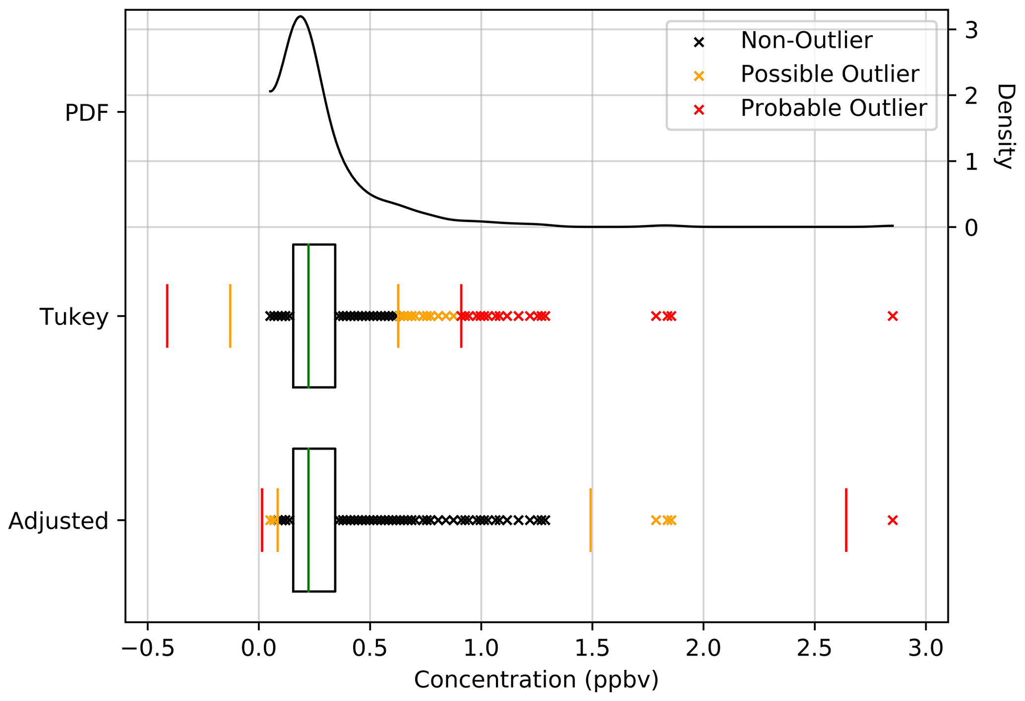
Figure 6 Illustration of the determination of possible (orange) and probable (red) data outliers using the Tukey boxplot and adjusted boxplot methods, for hourly NO₂ data in January 2018 at the suburban ES0013R_CL(IPC) station, Peñausende, Spain. Also shown is the probability density function of the data in the month.

3.5.2 Monthly distribution consistency

Data outliers are most commonly thought of as values which are far from all other values. However, data can also be outlying as a collective. For example, the measurements in the month of July of one year can be significantly different from the collections of measurements in all previous Julys. These types of outliers can be entirely real in origin, e.g. driven by extreme meteorological conditions, or can be erroneous, e.g. due to measurement issues. In either case, these types of outliers should be flagged in some way.

One way of checking for these outliers is to look at how the data distribution for one specific month, e.g. July 2016, at a station compares with the distributions for the same month, i.e. July, across the years. If one month's distribution is extremely different from the typical monthly distribution, this is obviously suspicious and should be flagged. The efficacy of this method is affected by long-term trends changing the station's distribution over time, but the impact of this can be constrained by only comparing against distributions in a limited range of years. Additionally, the variability of the distributions over time may vary significantly from station to station, which needs to be accounted for.

To allow for the quantification of the comparison of data distributions in different months, kernel density estimation is used to estimate the probability density function (PDF) of the data in each month. The intersection of the PDFs of two separate months can be used to objectively measure the consistency of monthly data distributions. An intersection score between 0.0 and 1.0 is returned, 0.0 being no intersection and 1.0 being a perfect intersection. A PDF is only estimated for any given month when there are ≥100 valid values after screening by other GHOST QA flags (defined in Table A14) and when there is a minimum of three unique values in the month to ensure that there are sufficient values of quality to estimate the PDF.

We attempt to estimate the consistency of the distribution for one specific month, termed the target month, with the distributions for the same month (e.g. July) across the years. By calculating the intersections of the PDF for the target month with PDFs of the same month in the surrounding ±5 years, a metric for the short-term consistency of the target month is obtained. This is calculated by

$$\begin{array}{}\text{(10)}& C_{\mathrm{ST}}=\mathrm{1.0}-\stackrel{\mathrm{̃}}{I},\end{array}$$

where C_ST is the short-term consistency and $\stackrel{\mathrm{̃}}{I}$ is the median intersection of the PDF for the target month with PDFs of the same month in the surrounding ±5 years.

The short-term consistency ranges between 0.0 and 1.0. A score of 0.0 indicates that the target month's data are perfectly consistent with a typical month, and a score of 1.0 indicates that it has no consistency with a typical month.

If the PDF for the target month cannot be estimated or there are less than two estimated PDFs in total across the surrounding years, there is not enough information to accurately assess the consistency of the target month's data, and a GHOST QA flag is written informing of this: “Monthly Distribution Consistency – Unclassified” (code 130).

By calculating the median short-term consistency of the same month as the target month (e.g. July) over the time record, a measure for the standard consistency is obtained. When referenced against the short-term consistency, this gives a metric for the deviation of the short-term consistency from the standard consistency, termed the deviation of consistency. This is calculated by

$$\begin{array}{}\text{(11)}& C_{\mathrm{D}}={\stackrel{\mathrm{̃}}{C}}_{\mathrm{ST}}-C_{\mathrm{ST}},\end{array}$$

where C_D is the deviation of consistency and ${\stackrel{\mathrm{̃}}{C}}_{\mathrm{ST}}$ is the median short-term consistency of the same month over the time record, termed the standard consistency.

The deviation of consistency is normalised after calculation. If the score is less than 0.0, it is set to 0.0, i.e. any case where the short-term consistency for the target month is equal to or greater than the standard consistency. Next, the score is scaled to be a ratio to the standard consistency. The deviation of consistency ranges between 0.0 and 1.0. A score of 0.0 indicates that the short-term consistency is equal to or greater than the standard consistency, and a score of 1.0 indicates that the short-term consistency is as far below the standard consistency as it can possibly be.

Finally, the short-term consistency and deviation of consistency are summed to give a final consistency score for the target month:

$$\begin{array}{}\text{(12)}& C=C_{\mathrm{ST}}+C_{\mathrm{D}},\end{array}$$

where C is the consistency score.

The consistency score ranges between 0.0 and 2.0, where 0.0 indicates that the target month has an extremely typical distribution and 2.0 indicates that the target month has an extremely atypical distribution. The score is split into 10 zones (in range increments of 0.2), from the most typical distributions in Zone 1 (scores of 0.0 to 0.2) to the most atypical distributions in Zone 10 (scores of 1.8 to 2.0). All months for which a consistency score can be determined are associated with the appropriate GHOST QA flag “Monthly Distribution Consistency – Zone [N]” (codes 120–129), where [N] is the zone number of the consistency score. If 2/3, 4/6, or 8/12 consecutive months are classed as Zone 6 or higher, it is suspected that there is a systematic reason for the atypical distributions, and the whole periods are flagged with the appropriate GHOST QA flags “Systematic Inconsistent Monthly Distributions – 2/3 Months ≥ Zone 6” (code 131), “Systematic Inconsistent Monthly Distributions – 4/6 Months ≥ Zone 6” (code 132), and “Systematic Inconsistent Monthly Distributions – 8/12 Months ≥ Zone 6” (code 133).

Figure 7 visually describes this classification procedure for hourly O₃ data at a rural background station, Cabo Verde, for two different months: July 2009 and July 2012. The distribution of data in July 2009 is markedly different from the July data of the surrounding years, whereas the distribution in July 2012 is very similar to the surrounding years. July 2009 is classified as being Zone 10, an extremely atypical July, whereas July 2012 is classified as Zone 2, a very typical July.

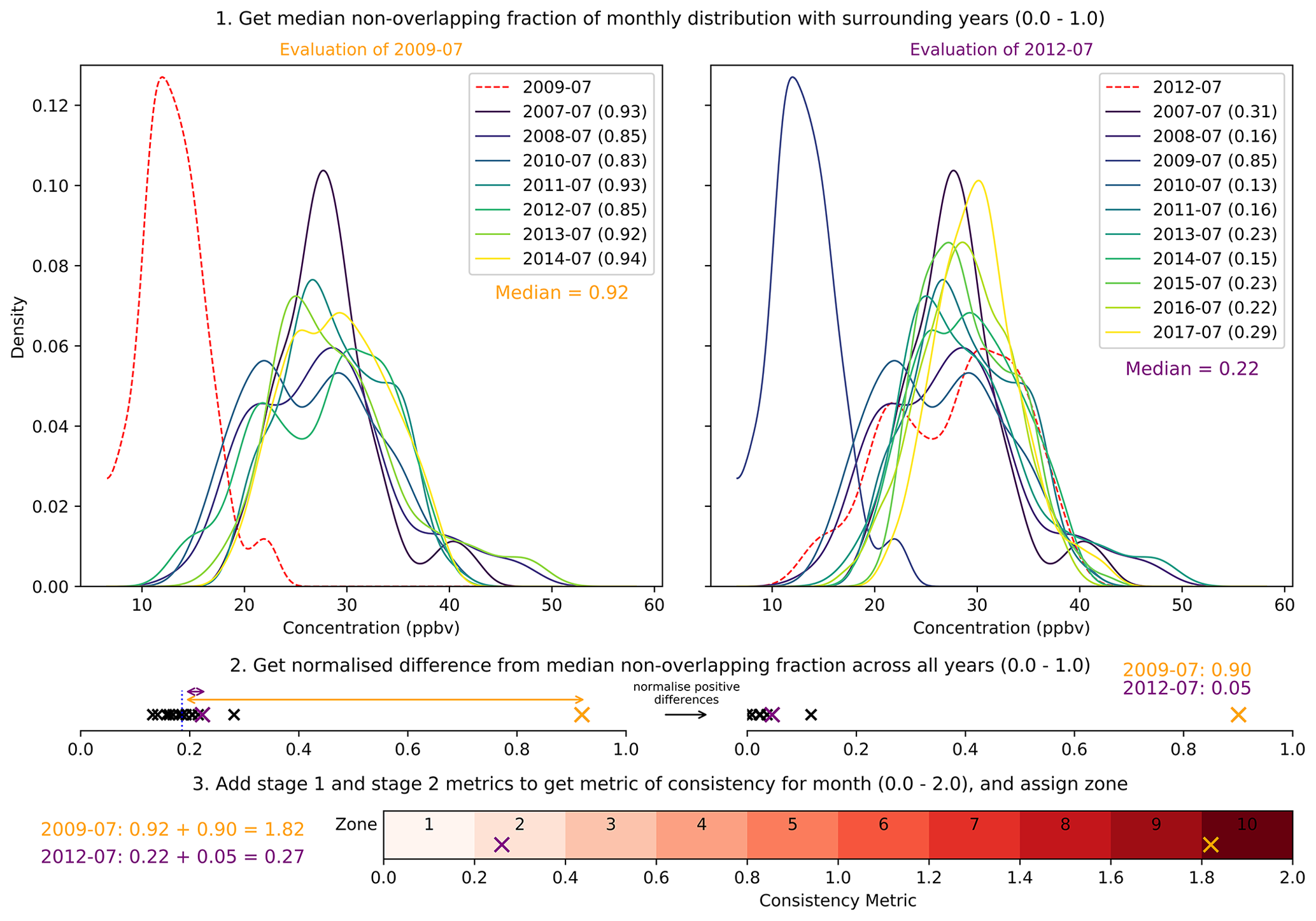
Figure 7 Illustration of the procedure for classifying the consistency of a monthly distribution of measurements with other distributions for the same month across the years. The classification is demonstrated for hourly O₃ data at the rural background CV0001G_UVP station, Cabo Verde, in two different months: July 2009 and July 2012. The distribution of data in July 2009 is markedly different from the July data of the surrounding years, whereas the distribution in July 2012 is very similar to the surrounding years. July 2009 is classified as being Zone 10, an extremely atypical July, whereas July 2012 is classified as Zone 2, a very typical July.

3.5.3 Pre-filter data by default GHOST quality assurance

Although the extensive number of GHOST and network QA flags gives users a wealth of options for filtering data, in many cases users simply want reliable data, with no major outliers and without having to worry about how to filter data. Therefore, such an option is provided, pre-filtering data by some default GHOST QA defined in Table A10. These QA flags are chosen conservatively, intending to remove only probable invalid values. Therefore, greater filtering may be required to solve other data issues. This is saved to the data variable “GHOSTcomponentname_prefiltered_defaultqa”, where GHOSTcomponentname is the standard GHOST name for the component as defined in Table 2.

3.6 Add temporal classifications (Stage 5)

When evaluating station data, to better understand the driving temporal processes at play, it is common to screen data by some form of temporal classification, e.g. day/night. Thus, to streamline this process for end-users of GHOST, some of the most widely used temporal classifications are calculated and associated with station measurements. These are the day/night, weekday/weekend, and season classifications.

These temporal classifications are added as data variables, with integer classification codes per measurement. Table 11 details the different temporal classification types, with a definition of the class codes and a description of the procedure used to calculate each of the classes. Whenever a temporal classification cannot be calculated, either because the temporal resolution is too coarse or the local time zone is unknown, a fill value (255) is set instead.

Parallelisation is done by unique station (via station_reference) in the stage.

(Rhodes, 2024)

Table 11 Summary of the temporal classification data variables in GHOST. For each variable, the associated classification codes, calculation requirements, and the procedure for calculation are given.

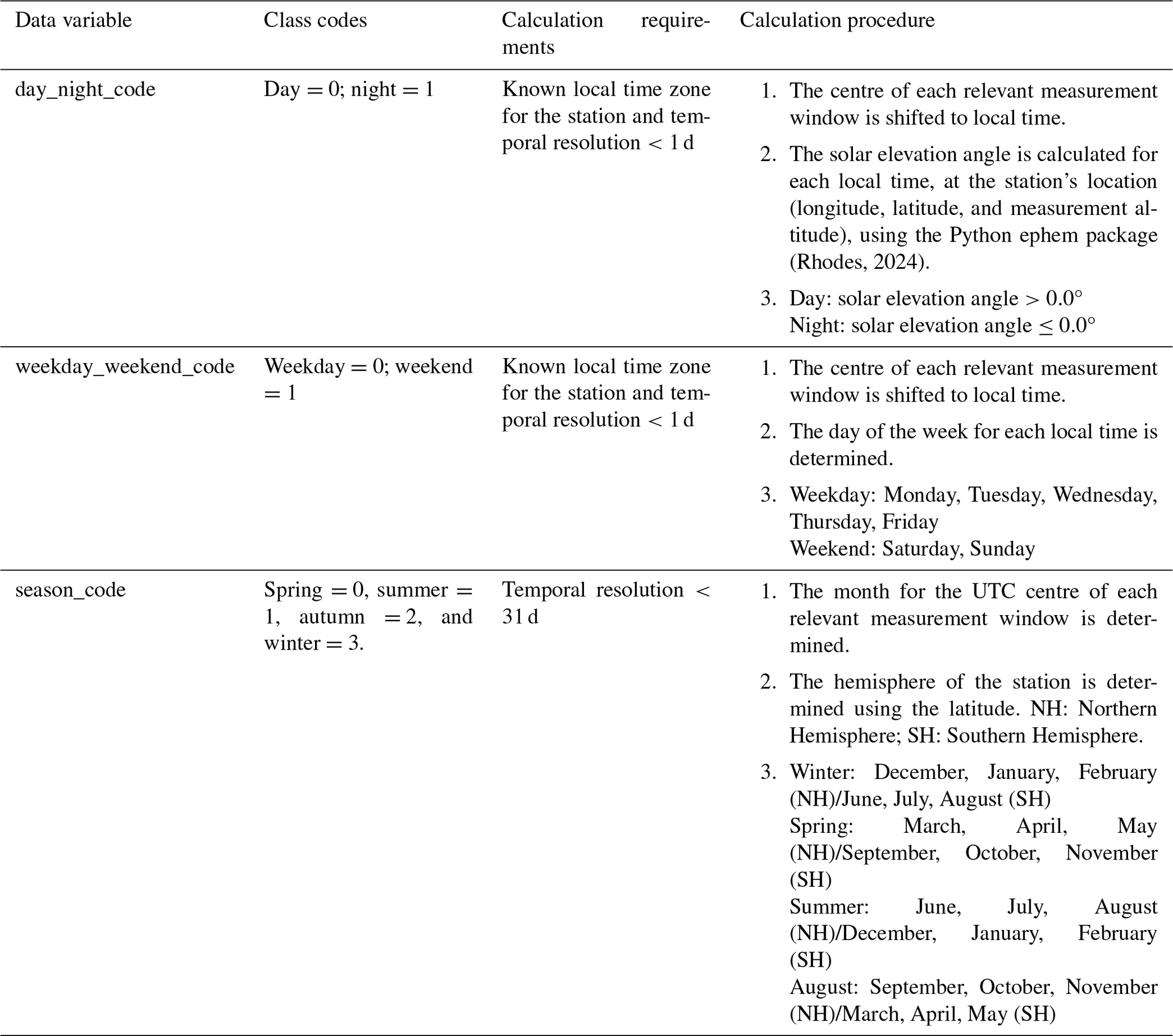
3.7 Temporally average data (Stage 6)

At this point in the pipeline, all reported station data and metadata for a component, for a given network, have been standardised, concatenated, and complemented with gridded metadata, GHOST QA, and temporal classifications. As measurements of all temporal resolutions are processed in GHOST (e.g. 30 min or 6 h), the data for each station can be composed of a variety of temporal resolutions.

In this stage, station measurements are temporally standardised, temporally averaging data to standard temporal resolutions, i.e. hourly, hourly instantaneous, daily, and monthly. Other data variables, e.g. data flags or temporal classifications, are also temporally standardised.

Data variables informing on the representativity of the temporal averaging are also created, providing the percentage representativity of the native measurements that goes into each temporal average. As well as having measurements associated with UTC, measurements are also associated with other reference times, i.e. mean solar time and local time.

Parallelisation is done by unique station (via station_reference) and standard temporal resolution (e.g. hourly or daily) pairings in the stage.

3.7.1 Temporal averaging procedure

First, station measurements with a coarser temporal resolution than the standard temporal resolution being averaged to are dropped. For example, monthly-resolution measurements are dropped when processing hourly averages. Stations with no remaining data after this are excluded from further processing for the particular standard temporal resolution.

Next, a regular grid of times between January 1970 and January 2023 is created, with the spacing between each time being the relevant standard temporal resolution, e.g. for a monthly resolution: 1 January 1970, 00:00, 1 February 1970, 00:00, 1 March 1970, 00:00, etc. These times are the start times of the temporally standardised measurements, which will be written out in the finalised netCDF4 file as the “time” data variable. Each consecutive pair of times represents the start point and end point of each measurement, which are termed the standard measurement windows.

For some components, measurements are representative of a moment in time rather than an average over time. All components that are not in the gas and particulate matrices, i.e. aerosol optical properties, have measurements which are instantaneous in nature. Measurements of this type are therefore extremely time-sensitive, and averaging these measurements without care could result in nonsensical output. For example, when calculating hourly averages, instantaneous measurements at 00:01 and 00:59 would be averaged together, despite the measurements being 58 min apart and potentially extremely different. To combat this, the hourly instantaneous resolution is added for all instantaneously measured components. For this resolution, the standard measurement windows are adjusted to be centred around the top of the UTC hour, e.g. 1 June 1970, 06:30; 1 June 1970, 07:30; 1 June 1970, 07:30; and 1 June 1970, 08:30. Rather than taking an average of the native measurements in each measurement window, the value closest to the top of each UTC hour is taken to represent the window.

The temporal standardisation process is now started. The standard measurement windows are iterated chronologically, and in each window a value for every data variable is set, e.g. measurements, data flags, or temporal classifications. How these values are set depends on the number of native-resolution measurements that overlap with each standard window. A native measurement can be entirely contained within a window, can be equivalent to the window (i.e. same start and end points), or can lie across the bounds of two or more windows.

If zero native measurements lie in a window, the measurement value of the window is set to be NaN. For the qa variable, the value is set as the GHOST QA flags that were set in the last window with a valid measurement, plus the “Missing Measurement” flag (code 0). This is done to ensure that the GHOST QA flags do not jump wildly through the time record, but it creates the assumption that the previously set flags are still applicable for the current window. All other data variable values are set to be NaN.

If there is just one native measurement in the window, that measurement is taken to represent the entire window. The other data variables are also taken as they are.

If there is more than one native measurement in the window, a procedure is undertaken to assign a measurement value for the window and assign values for the other data variables:

1. Invalid native measurements are first screened out using a defined set of GHOST QA flags in the “Invalid QA” grouping in Table A15. This tries to ensure that any temporal average is not biased by erroneous data. The reciprocal values of the invalid native measurements across the other data variables are also screened out.

2. If there are zero remaining native measurements after screening, then, for the hourly instantaneous resolution, the filtering is unapplied to ensure a value will be set for the window. For non-instantaneous resolutions, the measurement value of the window is set as NaN. For the qa variable, the value is set to be the GHOST QA flags that were set in the last window with a valid measurement, plus the “No Valid Data to Average” flag (code 8). All other data variable values are set as NaN, and processing proceeds to the next standard measurement window.

3. If there are remaining native measurements after screening for the hourly instantaneous resolution, the measurement closest to the UTC hour is simply taken to be the value for the window. The reciprocal value of the chosen measurement in all the other data variables is taken to set their values, and processing proceeds to the next standard measurement window.

4. If there are remaining native measurements after screening for non-instantaneous resolutions, the measurement value is set by taking a weighted average of the measurements in the window, with the weights being the number of minutes represented in the window per measurement. Values for the variables reported_uncertainty_per_measurement and derived_uncertainty_per_measurement are also calculated in the same way after excluding NaNs.

5. For the qa variable, GHOST QA flags that were used to screen measurements in step 1 are dropped. Other flags are kept if they appear more often than not in the window (i.e. modally). These other flags are defined in the “Modal QA” grouping in Table A15.

6. For the flag variable, all network QA flags are dropped as these have already been indirectly filtered by the GHOST QA flag “Invalid Data Provider Flags – GHOST Decreed” (code 6) in step 1. The “Valid Data” flag (code 0) is then set solely for the window.

7. For each of the “day_night_code”, “weekday_weekend_code”, and “season_code” variables, the weighted mode over the respective codes in the window is taken to set their value, with the weights being the number of minutes represented in the window per associated measurement.

After all standard measurement windows have been iterated through, the station data have been completely temporally standardised.

3.7.2 Calculate temporal representativity

In parallel to the temporal averaging procedure, calculations of the temporal representativity of the native measurements across a variety of temporal periods are made. This is done as it is very useful, and often important, to know the representativity of the native measurements used for creating temporal averages. The different temporal periods evaluated are hourly, daily, monthly, and annual. The representativity is only calculated for periods as coarse as or finer than the standard temporal resolution. For example, for monthly averaged measurements, the evaluated periods would be monthly and annual.

All of the evaluated periods begin and end on UTC boundaries and start in January 1970, going through to January 2023. For example, for the hourly period, 1 January 1970, 00:00–1 January 1970, 01:00 UTC and 1 January 1970, 01:00–1 January 1970, 02:00 UTC would be the first two hourly periods evaluated.

For each temporal period, two metrics of representativity are calculated. The first metric is data completeness, i.e. the percentage of the relevant period that is represented by native measurements. The second metric is the maximum data gap, i.e. the percentage maximum data gap in the relevant period that is filled with native measurements relative to the total period length. All representativity percentages are returned as rounded integers (0 %–100 %).

If the temporal resolution is hourly instantaneous, the representativity calculations are modified slightly. Rather than calculating the representativity over the total period, it is calculated as the percentage of all standard temporal-resolution windows inside the relevant period that contain native measurements.

The calculated representativity variables are written to data variables with the syntaxes “[period]_native_representativity_percent” and “[period]_native_max_gap_percent”, where [period] is replaced with the relevant temporal period, e.g. annual. All representativity variables are saved at the standard temporal resolution. For example, if the standard temporal resolution is hourly and the evaluated temporal period is annual, each annual UTC period is divided into hourly chunks and all chunks are assigned the calculated representativity metric for the annual period.

3.7.3 Local and mean solar time

As well as having measurements referenced to UTC, it is often useful to have measurements referenced to different time standards. As referenced previously, time manipulation is often a non-trivial affair, and to ensure that end-users do not need to calculate this, station measurements are referenced against two other widely used time standards: local time and mean solar time.

Local time is defined simply as the local time at each station at the time of measurement. This is calculated by converting the standard UTC times using the pytz Python package (Bishop, 2024), fed with the local time zone determined in Sect. 3.4.5. The calculated times are written to the “local_time” data variable. Unlike the standard UTC “time” variable, these times vary by station.

Solar time is defined as the time measured by Earth's rotation relative to the Sun. Apparent solar time is determined by direct observation of the Sun, whereas mean solar time is the time that would be measured by observation if the Sun travelled at a uniform apparent speed throughout the year rather than slightly varying across the seasons. More technically, it is defined as the hour angle of the mean Sun plus 12 h. The hour angles of each of the standard UTC times are calculated using the Python ephem package (Rhodes, 2024) and station longitude. The calculated times are written to the “mean_solar_time” data variable. These times also vary by station.

3.7.4 Station netCDF creation by year and month

At this point, the associated data by station have been temporally standardised and are ready to be saved to their finalised form. Station data, as per the standard temporal resolution, are grouped by year and month. Due to GHOST metadata being dynamic, it is possible for there to be multiple values associated with a metadata variable in a month. For the purpose of simplicity, it was decided to limit the number of values associated with each metadata variable in a month to just one. If there is more than one unique value for any metadata variable in a month, the value which is representative of the greater number of minutes in the month is chosen to represent the variable. The data and metadata in each group are then written to a station-specific netCDF4 file for the relevant year and month. Station-specific files are written are for all year and month groups which contain station data.

All information associated with the data and metadata variables written in the netCDF4 files, e.g. variable names or data types, is defined in Tables A1 and A2 respectively.

3.8 Monthly aggregation by station (Stage 7)

Once all station-specific netCDF4 files have been written for a network and component pair, the last remaining task is to aggregate the files. All station-specific netCDF4 files of the same standard temporal resolution, by year and month, are aggregated into one netCDF4 file using NCO (The NCO Project, 2024). The resultant filenames have the form “GHOSTcomponentname_YYYYMM.nc”, where GHOSTcomponentname is the standard GHOST name for the component as defined in Table 2. This is the finalised form of the GHOST data that are separated by network.

Parallelisation is done by year and month, together with the standard temporal-resolution pairings in the stage.

3.9 Cross-network synthesis (Stage 8)

At this point in the pipeline, finalised netCDF4 files for a component, for all standard temporal resolutions, across all the networks have been written. In order to maximise the usefulness of GHOST, with model evaluation specifically in mind, component data across all the networks are synthesised, resulting in a unified “network”. This synthesis is done by year, month, and standard temporal resolution.

During this process, any duplicate stations across the networks are identified, and one is kept preferentially. The preference is made by prioritising some networks over others, with these determinations made using the experiences gleaned while processing data from each of the individual reporting networks in this work. These network preferences are not disclosed here out of respect to the data providers.

Identifying duplicate stations is done by geographically matching stations within a tolerance of 19.053 m. This tolerance is calculated by allowing for a tolerance of 11 m in each of the three independent x, y, and z dimensions, as is done in Stage 2 of the GHOST pipeline to distinguish unique stations. Station longitudes, latitudes, and measurement altitudes are converted to Earth-centred, Earth-fixed (ECEF) coordinates, and the distances between all the stations are then calculated. Any geographically matched stations which use different measurement methods are not classed as duplicates.

The resultant filenames have the same syntax as the finalised network-specific files described in Sect. 3.9 but are saved under the synthesised network name “GHOST-PUBLIC”.

Parallelisation is done by year and month as well as the standard temporal-resolution pairings in the stage.

4 Finalised datasets

In this section, the file structure of the finalised GHOST dataset is detailed, and the temporal and spatial data extent for some key variables is described.

The GHOST dataset is made freely available via the following repository: https://doi.org/10.5281/zenodo.10637449 (Bowdalo, 2024a).

The dataset consists of a total of 7 275 148 646 measurements from 1970–2023, 227 different components, and 38 reporting networks.

The data are available in two forms. The first form is separated out by network and component. The second form is a synthesis across networks by component and is saved under the GHOST-PUBLIC name. Data are saved for both forms as netCDF4 files, by year and month and at four different temporal resolutions: hourly, hourly instantaneous, daily, and monthly. The dataset includes data from all networks that we have the right to redistribute, which are indicated in the “Data rights” column of Table 1.

Figure 8 shows the temporal data availability in GHOST of four key components: O₃, NO₂, CO, and total PM₁₀. The evolution of the number of stations, by network, is shown across the time record (for monthly-resolution data). The earliest measurements made for O₃ are from 1970 from the Japan NIES network. In general, the total number of stations has increased steadily across time for all the components. However, there is a large variation in the station numbers across the networks. The networks with the largest station numbers are those which exist for regulatory purposes, i.e. those which exist to monitor compliance with national or continental air quality limits (e.g. EEA AQ e-Reporting, Japan NIES, or U.S. EPA AQS).

In 2012 there was a major transition in the reporting framework of the major European database, which exists to monitor the air quality compliance of EU member states. The framework name changed from EEA AirBase to EEA AQ e-Reporting and is treated in GHOST as two separate networks. Thus, this crossover is evident in Fig. 8, as EEA AQ e-Reporting station numbers ramped up over 2012 and EEA AirBase went offline in 2013.

For O₃, there is a clear seasonal trend in the number of stations from the U.S. EPA's AQS network, with the numbers increasing in the summer and then decreasing in the winter. This is because the stations in the U.S. EPA's AQS primarily monitor O₃ to check for air quality compliance, which is typically only of concern in the summer, when more light is available to drive O₃ production. Interestingly, the number of stations for CO and PM₁₀ in the U.S. EPA's AQS network have dropped significantly since the 1990s.

Figure 9 shows the spatial data availability in GHOST of the same four key components across the entire 1970–2023 time range, i.e. the unique stations by network over the time record. There is excellent spatial coverage in North America, Europe, and eastern Asia across the components. However, there are consistent spatial gaps over Africa, central Asia, and South America (excluding Chile). In general, there is a large disparity between the number of stations in the Northern Hemisphere and the Southern Hemisphere. This disparity is less prevalent for CO, with the inclusion of flask samples from the WMO GAW WDGGG network providing excellent spatial coverage. Stations in networks which exist to measure rural background concentration levels (e.g. the U.S. EPA's CASTNET) are far less densely distributed than they are in regulatory networks (e.g. the U.S. EPA's AQS), where stations are mostly located in urban areas.

Figure 8 Evolution of the number of stations in GHOST in each month across the time record (1970–2023) for four key components: O₃, NO₂, CO, and PM₁₀. The differing number of stations per reporting network are represented by differently coloured lines. The total number of stations across all the networks is shown in black.

Figure 9 Spatial distribution of all unique stations in GHOST across the time record (1970–2023) for four key components: O₃, NO₂, CO, and PM₁₀. The stations are coloured by reporting network. The number of unique stations across the time record, per component, is given in the map titles.

5 Recommendations for data providers

The measurement of atmospheric components can often be costly and requires a huge amount of human labour, especially when low measurement uncertainty is required. We would like to thank all the data providers for their work, which is of great benefit to the entire atmospheric composition community. The work done in creating GHOST however has highlighted several issues associated with the reporting of atmospheric composition data. In this section we will highlight some issues we identified through this work, which we hope will be useful feedback for data providers.

In general, despite extensive efforts to gather as much available information from each reporting network as possible, there is simply a lack of detailed metadata associated with measurements. This lack of detail leads to many assumptions being made and subsequently uncertainties being placed onto measurements. In many cases, even basic metadata, such as the measurement altitude, sampling height, or even longitude and latitude, are not provided. Even when metadata are provided, the lack of explicit detail can also lead to significant uncertainties. For example, providing a longitude and latitude with just a couple of decimal places can lead to the measurement position being erroneously located tens of kilometres from the correct position. This was found to happen even to one of the most famous measurement stations, with its position being erroneously stated to be over the ocean.

The area where the reported metadata are most lacking is that associated with measurement processes. In the majority of cases, the only measurement process information provided is a measurement methodology, and in some instances even that is not provided. Information such as the instrument name, sampling procedures, and limits of detection is very rarely provided, and more advanced information about measurement uncertainties or calibration procedures is almost never provided. Even when metadata are available, the lack of harmonisation across the reporting networks imposes a significant strain on the processing. For example, there are a number of methodologies which fundamentally measure concentrations of total PM through the scattering of visible light, i.e. nephelometry, light scattering photometry, and optical particle counting. Each of these methods operates in subtly distinct ways, and simply stating “light scattering” is not enough information to determine exactly which method was used.

The conversion of measurement units was also made very challenging by the limited information that was available. In some cases the reported units were not provided with the data or metadata and required rigorous investigation of network reports to find. When converting from a mass density (e.g. µg m⁻³) to a mole fraction (e.g. ppbv) or vice versa, the conversion requires the temperature and pressure associated with the air sampled. An additional complication is that many networks standardise measurements to a fixed temperature and pressure. The sample or network standard temperature and pressure are not commonly reported across the networks, and in some cases assumptions were needed to be made when converting units. Ideally, data providers would reference the applicable international measurement standards for their measurements, e.g. European standards.

The lack of metadata, for each of the cases outlined here, could probably be easily remedied by the data providers, as they most likely already have most of the information. A more deep-rooted issue however is the reporting format used by networks to provide metadata. In the majority of the cases, station metadata are provided in an external file and are applicable for the entire time record. For stations which have measured for decades this can be problematic, as the type of air predominantly sampled at a station can evolve over time and should be reflected in the metadata, e.g. through station classes. Measurement techniques are also ever-evolving, and thus instrumentation is continuously being replaced or upgraded, which should also be reflected in the metadata.

One promising approach, which has been adopted by the EEA AQ e-Reporting network, is to associate all measurements with a sample ID. Each ID is associated with a specific collection of metadata, e.g. longitude, measurement method, or instrument name. If one of the metadata values in this collection changes, e.g. when a new instrument is installed, the previous ID is no longer applicable and a new ID is associated with the measurements. Such an approach allows for the reporting of measurements from multiple instruments at one station. A potentially even cleaner approach would be to have a set of IDs for metadata associated with the station position, i.e. longitude, latitude, or sampling height, and another set of IDs for metadata associated with measurement processes. This would ensure that a large number of metadata values are not needlessly duplicated between IDs when just one value changes.

6 Data availability

The GHOST dataset is made freely available via the following repository: https://doi.org/10.5281/zenodo.10637449 (Bowdalo, 2024a). The dataset has been licensed with CC BY 4.0. We kindly ask any use of this dataset to cite both this publication and the dataset itself.

The dataset is 1.39 TB in total size (121 GB compressed) and includes data from all networks that we have the right to redistribute, which is indicated in the “Data rights” column of Table 1. The specific network data sources that GHOST draws from are listed in Table 1.

The data are separated out by network, temporal resolution, and component and are saved as netCDF4 files by year and month. There is additionally one synthetic network entitled GHOST-PUBLIC, which aggregates data across all the networks. The dataset is compressed as .zip files by network. Beneath each network, collections of files by temporal resolution and component are compressed as tar.xz files.

Each network .zip file can be decompressed using the following syntax: unzip [network].zip.

Component tar.xz files can be decompressed using the following syntax: tar -xf [component].tar.xz.

7 Code availability

The software used to process GHOST is available from Zenodo (https://doi.org/10.5281/zenodo.13859074, Bowdalo, 2024b) under a LGPLv3 licence.

8 Conclusions

GHOST represents one of the biggest collections of harmonised measurements of atmospheric composition at the surface. In total, 7 275 148 646 measurements from 1970 to 2023, 227 different components, and 38 reporting networks are compiled, parsed, and standardised. The components processed include gaseous species, total and speciated particulate matter, and aerosol optical properties. The data are made available in netCDF4 files at four different temporal resolutions: hourly, hourly instantaneous, daily, and monthly.

The main goal of GHOST is to provide a dataset that can serve as a basis for the reproducibility of model evaluation efforts across the community. Exhaustive efforts have been made to standardise almost every facet of the information provided by the major public reporting networks. This has been saved in 21 data variables and 163 metadata variables. For this purpose, a fully parallelised workflow was created to enable the processing of such a large quantity of data. Through this process, a number of challenging issues are tackled, e.g. converting measurement units, shifting local time to UTC, or handling measurement position changes. Extensive effort in particular is made to standardise measurement process information and station classifications.

Rather than dropping any measurements which are labelled as potentially erroneous by the measurement provider, a range of standardised network QA flags is associated with each individual measurement. GHOST's own QA is also performed and associated with measurements. For users who do not wish to worry about filtering data with the provided flags, measurements pre-filtered by some default GHOST QA are also provided.

Measurements of all temporal resolutions are parsed in GHOST (e.g. 30 min or 6 h) and are subsequently standardised by temporally averaging data to standard temporal resolutions (e.g. hourly). Data variables showing the representativity of the temporal averaging are created, providing the percentage representativity of the native measurements that go into each temporal average. A variety of different reference times are associated with the measurements: UTC, mean solar time, and local time.

Extra complementary information is also associated with measurements, such as metadata from various popular gridded datasets (e.g. land use) and temporal classifications per measurement (e.g. day/night). As the dataset spans more than 50 years, the metadata are handled dynamically and allowed to vary through the record, allowing changes in things such as the measurement instrumentation or measurement position to be tracked.

We hope this work can be a spark for greater dialogue in the community regarding the reporting and standardisation of atmospheric composition data and, rather than being just a one-off harmonisation effort, can be built upon and refined with the help of measurement experts from across the globe. We warmly encourage any data providers who wish to incorporate their data into GHOST to please contact us.

The GHOST dataset is made freely available from the following repository: https://doi.org/10.5281/zenodo.10637449 (Bowdalo, 2024a).

Appendix A

(Taylor et al., 2014)

Table A1 Definitions of GHOST standard data variables. The variable name, data type, and units as well as a brief description are given. The “Standard component units” refer to the standard units per component as documented in Table A3.

(Michelfeit, 2024)(Thampi, 2024)(Thampi, 2024)(Thampi, 2024)(Thampi, 2024)

Table A2 Definitions of GHOST standard metadata variables. The variable name, data type, and units as well as a brief description are given. The “Standard component units” refer to the standard units per component as documented in Table A3.

Table A3 GHOST standard component information grouped by matrix. For each component, the chemical formula, long component name, standard units, minimum permitted measurement resolution, extreme lower limit, extreme upper limit, and extreme upper monthly median are given.

Table A4 Definitions of the fields associated with each GHOST standard station classification metadata variable. Some of the fields also contain sub-fields where extra information from the data provider allows for finer-grained classification.

Table A5 Outline of the GHOST standard sampling types, with a description given for each type. These are set in the “primary_sampling_type” and/or “measuring_instrument_sampling_type” variables, depending on the measurement process. For each type there are several standardised primary sampling instruments (83 in total across the types) set in the “primary_sampling_instrument_name” variable. Measurements utilising a primary sampling instrument of a type that they are not associated with are given the “Erroneous Primary Sampling” (code 20) GHOST QA flag. Measurements utilising a primary sampling instrument whose type or name is unknown are given the “Unknown Primary Sampling Type” (code 14) and “Unknown Primary Sampling Instrument” (code 15) GHOST QA flags respectively. Any measurements where any assumptions are made regarding the primary sampling are given the “Assumed Primary Sampling” (code 11) GHOST QA flag.

Table A6 Outline of the GHOST standard sample preparation types and techniques, with a description given for each type. These are set in the “sample_preparation_types” and “sample_preparation_techniques” variables. Each preparation type can have multiple sub-techniques. Measurements which use a preparation type that they are not associated with are given the “Erroneous Sample Preparation” (code 21) GHOST QA flag. When sample preparation of a given type or technique is utilised but is unknown, measurements are given the “Unknown Sample Preparation Type” (code 16) and “Unknown Sample Preparation Technique” (code 17) GHOST QA flags respectively. Any measurements where any assumptions are made regarding the sample preparation are given the “Assumed Sample Preparation” (code 12) GHOST QA flag.

Table A7 Outline of the GHOST standard measurement methods, set in the “measurement_methodology” variable. Associated with each method is an abbreviated code (e.g. UVP), which is also included in the “station_reference” variable (e.g. AHP_UVP). For each method, the associated default sampling type and sample preparation are stated; these are set in the “measuring_instrument_sampling_type” and “sample_preparation_types” variables respectively. Also stated are the components that each method is known to measure and the components which are accepted by GHOST QA for measurement (i.e. without major known biases). For each method there are several standardised instruments that employ it (508 in total across the methods), set in the “measuring_instrument_name” variable. Components measured with a method they are not associated with or a method not accepted by GHOST QA are given the “Erroneous Measurement Methodology” (code 22) and “Invalid QA Measurement Methodology” (code 23) GHOST QA flags respectively. Measurements for which the methodology or measuring instrument is unknown are given the “Unknown Measurement Method” (code 18) and “Unknown Measuring Instrument” (code 19) GHOST QA flags respectively. Any measurements where any assumptions are made regarding the method are given the “Assumed Measurement Methodology” (code 13) GHOST QA flag.

Table A8 Definitions of the standardised network QA flags, set in the flag variable. These flags represent a standardised version of all the different QA flags identified across the measurement networks. Whenever a flag is not active, a fill value (255) is set instead.

Table A9 Definitions of GHOST QA flags, set in the qa variable, each derived from GHOST's own quality control checks. Whenever a flag is not active, a fill value (255) is set instead.

Table A10 Definition of the default GHOST QA flags used to pre-filter data to create the GHOSTcomponentname_prefiltered_defaultqa data variable. The QA flag code and name are both stated.

(NASA et al., 2018)(NOAA NGDC, 2009)(Crippa et al., 2018; EC JRC and Netherlands PBL, 2017)(Iwahashi and Pike, 2007; ESDAC, 2024)(Meybeck et al., 2001; ESDAC, 2024)CIESIN and CIAT (2005)CIESIN (2018)(Corbane et al., 2018, 2019)(Freire et al., 2016; Schiavina et al., 2019)(Ehrlich et al., 2019; Pesaresi et al., 2019)(NASA OBPG, 2024)(Beck et al., 2018)(Friedl and Sulla-Menashe, 2015)(Friedl and Sulla-Menashe, 2015)(Friedl and Sulla-Menashe, 2015)(NOAA and US Air Force Weather Agency, 2024)(Krotkov et al., 2017, 2019)(Krotkov et al., 2017, 2019)(Krotkov et al., 2017, 2019)(Krotkov et al., 2017, 2019)(WMO, 2024a)(Olson et al., 2001)(Olson et al., 2001)(Olson et al., 2001)(Ellis et al., 2010; University of Maryland Baltimore County, 2024)

Table A11 Description of the gridded metadata which are ingested in GHOST. This is an expanded version of Table 9, giving for each metadata type the temporal and spatial extents, the ellipsoid or projection, the horizontal or vertical datum, the native horizontal resolution, and the native file format.

Table A12 Outline of the key metadata variables (grouped by type) used for the assessment of duplicate metadata columns in Stage 1 of the GHOST pipeline (standardisation). A metadata column is identified as being “duplicate” if none of the key variables changes from the previous column.

Table A13 Definitions of the dependencies for the temporal filling of metadata variables in Stage 2 of the GHOST pipeline (station data concatenation) to prevent incompatibilities in concurrent metadata variables. This essentially means, for all metadata variables in a group, that each variable can only be filled temporally (going either forwards or backwards in time) if none of the dependent variables has changed between the metadata columns. Because of the importance of positional variables being set (e.g. latitude), filling is attempted through several passes, using progressively less stringent dependencies until it ultimately requires no dependencies. The “non-filled” group outlines variables that filling is not performed for due to it being highly time-sensitive.

Table A14 Outline of all GHOST QA checks in Stage 4 of the GHOST pipeline (quality assurance), which pre-screen data by another GHOST QA before calculation.

Table A15 Outline of the different GHOST QA flag groupings in Stage 6 of the GHOST pipeline (temporal averaging), detailing how GHOST QA flags are treated whenever measurements are averaged in a window. When averaging measurements, some GHOST QA flags are applied to screen invalid data, whereas the rest of the flags are only retained if they appear more than not across the window.