the Creative Commons Attribution 4.0 License.
the Creative Commons Attribution 4.0 License.
 | 13 Sep 2024
Climate and ablation observations from automatic ablation and weather stations at A. P. Olsen Ice Cap transect, northeast Greenland, for May 2008 through May 2022
Daniel Binder
Anja Rutishauser
Bernhard Hynek
Robert Schjøtt Fausto
Michele Citterio
The negative surface mass balance of glaciers and ice caps under a warming climate impacts local ecosystems, influencing the volume and timing of water flow in local catchments while also contributing to global sea level rise. Peripheral glaciers distinct to the Greenland ice sheet respond faster to climate change than the main ice sheet. Accurate assessment of surface mass balance depends on in situ observations of near-surface climate and ice ablation, but very few in situ observations of near-surface climate and ice ablation are freely available for Greenland's peripheral glaciers. The transect of three automated weather and ablation stations on the peripheral A. P. Olsen Ice Cap in northeast Greenland is an example of these much needed data. The transect has been monitored since 2008, and in 2022, the old weather and ablation stations were replaced by a new standardized setup. In order to ensure comparable data quality of the old and new monitoring station setups, it is necessary to re-evaluate the data collected between 2008 and 2022. This paper presents the fully reprocessed near-surface climate and ablation data from the A. P. Olsen Ice Cap transect from 2008 to 2022, with a focus on data quality and the usability in ice ablation process studies. The usability of the data is exemplified by the data in an energy balance melt model for two different years. We show that the inherent uncertainties in the data result in an accurate reproduction of ice ablation for just one of the two years. A transect of three automatic ablation and weather stations of this length is unique to Greenland's peripheral glaciers, and it has a broad scale of usage from input to climate reanalysis and detailed surface ablation studies. The dataset can be downloaded at https://doi.org/10.22008/FK2/X9X9GN (Larsen and Citterio, 2023).
- Article
(6182 KB) - Full-text XML
- BibTeX
- EndNote


Under the influence of the current warming climate, glaciers and ice caps exhibit a pronounced negative surface mass balance, contributing significantly to sea level rise. Peripheral glaciers and ice caps that are separate from the Greenland ice sheet make up only about 4 % of Greenland's total glaciated area but are responsible for approximately 14 % of the island's current ice loss, contributing disproportionately to the overall ice reduction (Khan et al., 2022). What is equally as important is the set of local-scale changes occurring in glaciated catchments, where the volume and timing of meltwater affect the local environment both on land and in fjords and oceans. In situ observations of surface mass balance processes are important for understanding the effects of future climate change (e.g., Machguth et al., 2013). While the ablation zone of the Greenland ice sheet is well monitored by the in situ network of automatic weather stations run by the Programme for Monitoring of the Greenland Ice Sheet (PROMICE; Fausto et al., 2021) and the interior of the ice sheet is monitored by the Greenland Climate Network (GC-Net; Vandecrux et al., 2023), very few peripheral glaciers distinct from the Greenland ice sheet are being monitored. Due to the local effects of peripheral glaciers being in coastal areas with complex terrain, there is a marked difference in surface mass balance between peripheral glaciers and the main ice sheet (Abermann et al., 2019). Peripheral glaciers have already passed the tipping point for meltwater retention and runoff that the main ice sheet has yet to experience (Noël et al., 2017). This all sums up to a contribution to sea level rise from peripheral glaciers and ice caps that is disproportionately high compared to their area and mass relative to the main ice sheet (Bolch et al., 2013; Hugonnet et al., 2021).
The data presented here are from a transect of three Automatic Ablation and Weather Stations (AAWSs) located on the A. P. Olsen Ice Cap (referred to here as APO or the ice cap), northeast Greenland (Fig. 1). The transect is part of the GlacioBasis Zackenberg glaciological monitoring program, a sub-program of Greenland Ecosystem Monitoring (GEM; https://g-e-m.dk/, last access: 9 September 2024) at Zackenberg Research Station located in the Northeast Greenland National Park. GEM is an integrated monitoring and long-term research program focused on ecosystems, climate change effects, and feedback mechanisms in the Arctic. GEM covers three sites representing different zones of the Greenland Arctic area: Zackenberg in northeast Greenland (high Arctic), Disko Island in central West Greenland (a transition zone between the high Arctic and low Arctic), and Nuuk in southwest Greenland. The Zackenberg site is the longest-running site, with ecosystem monitoring active since 1995, and GlacioBasis Zackenberg is the longest-running glaciological monitoring program within GEM. APO was chosen for glaciological monitoring because it is the largest contributor of glacial meltwater into the Zackenberg River, which plays a crucial role in the downstream ecosystem, including the Young Sound ecology (Citterio et al., 2017; Sejr et al., 2022).
The first two AAWSs of the APO transect were installed in late April 2008 in the ablation zone, whereas the third AAWS was installed in August 2009 in the accumulation zone at the ice cap summit. The three AAWSs are the backbone of the glaciological monitoring, and a transect of three AAWSs is, to the best of the authors' knowledge, unique to Greenland. These three AAWSs have been running with alternating instrumentation until April 2022. In spring 2022, the installation of new standardized AAWSs, which are similar to the PROMICE and GC-Net stations (Fausto et al., 2021), was initiated. With the new standardized setup, the data from the APO transect will be handled as a PROMICE and GC-Net dataset, and data processing will be done using the Python package pypromice described in How et al. (2023). The purpose of this paper is to describe the dataset collected from the APO transect in the period before the standardized setup: May 2008 through May 2022. The variables published here are ice ablation, air temperature, relative humidity, air pressure, wind speed, and incoming and outgoing shortwave and longwave radiation, as well as AAWS tilt and snow depth and derived variables (cloud cover fraction, surface temperature, and albedo). These variables capture the major components of the surface energy balance, making the data useful for studying processes governing surface mass balance. Additionally, this dataset can be used to force and calibrate distributed surface ice ablation models such as the distributed surface energy balance model (Hock and Holmgren, 2005) or the coupled snowpack and ice surface energy and mass balance model in Python (COSIPY; Sauter et al., 2020). Furthermore, the variables are considered essential climate variables by the World Meteorological Organization's Global Climate Observing System (GCOS). The data from the APO transect have already provided valuable insights when combined with on-land climate observations from the Zackenberg Valley as demonstrated in studies on temperature slope lapse rates (Shahi et al., 2023) and the spatiotemporal variability in surface energy balance across different surface types (Lund et al., 2017).
The paper is organized as follows: Sect. 2 provides an overview of the study area, including logistical conditions for field visits. Section 3 details the data collection process and post-processing methods. Section 4 describes the quality control and data filtering procedures. Section 5 demonstrates the suitability of these data for energy balance calculations. Section 6 contains information about the processing scripts and data availability. Section 7 offers concluding remarks that summarize the paper.
APO is an ice cap with several glacier catchments extending in elevation from around 200 to 1500 m a.s.l., covering a total area of about 300 km2. The glacier catchment labeled east in Fig. 1, with Randolph Glacier Inventory (RGI) ID RGI60-05.20098 (RGI Consortium, 2017), is the main contributor of glacial meltwater to the Zackenberg River catchment and thus the area of focus for the glaciological monitoring (Fig. 1).
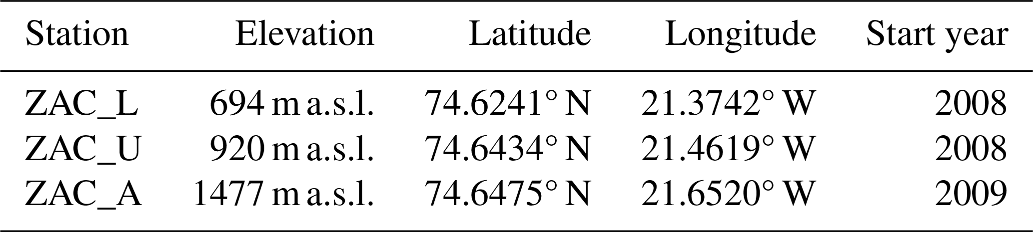
The APO transect consists of three AAWS sites (see Fig. 1 and Table 1): the lower site, ZAC_L (L for the lower ablation zone), has the longest and most complete data record. The middle site, ZAC_U (U for upper ablation zone), is located as close to the equilibrium line altitude as logistically possible and initially had a limited number of instruments. The top site, ZAC_A (A for accumulation zone), is located at the ice cap summit at an elevation of 1477 m. Due to COVID-19 pandemic travel restrictions in 2020 and 2021, the AAWS at ZAC_A was buried in 2020 and has not yet been recovered.
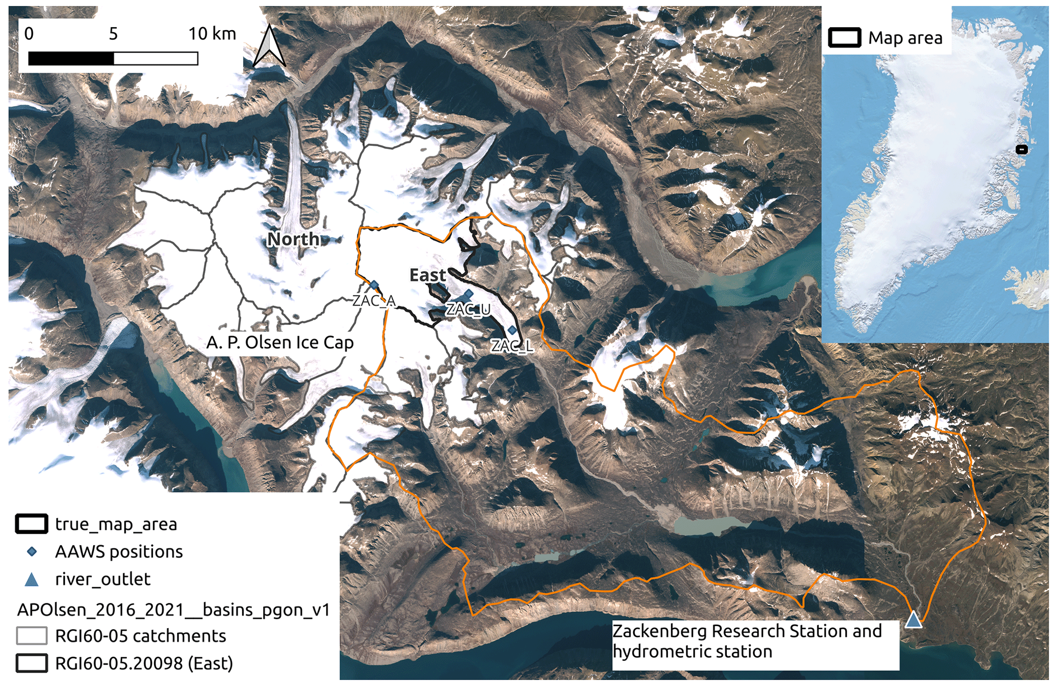
Figure 1A. P. Olsen Ice Cap outlined in individual glacier catchments that are modified slightly but follow the Randolph Glacier Inventory (RGI Consortium, 2017) and the hydrological catchment of Zackenberg River (orange outline). The base map is from the European Space Agency (ESA) Sentinel-2 satellite, taken in 2022; the Greenland overview in the insert is the background map from QGreenland, licensed under the Creative Commons Attribution 4.0 International License https://creativecommons.org/licenses/by/4.0/ (last access: 9 September 2024); the AAWSs are marked with blue diamonds; and the hydrometric station close to the river outlet is marked by a blue triangle. Maps are projected to UTM zone 27N.
Table 1Elevation, position, and monitoring start date of the three AAWSs on the A. P. Olsen transect.
Due to the remote location, the ice cap can mainly be reached by snow scooters traveling from Zackenberg Research Station, limiting the period where the glacier can be visited to the short period in spring after the end of polar night and before snowmelt, which is usually during the last 2 weeks of April. This means that the maintenance of the AAWSs is sensitive to snow conditions in April, and with the limited access, data gaps are inevitable.
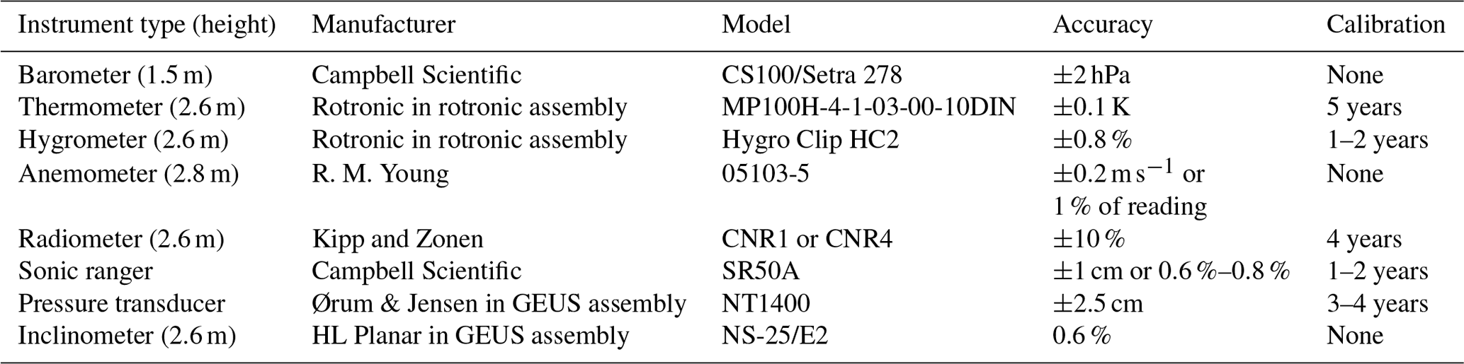
In this section, we describe the instrumentation on the AAWS and the steps taken to convert raw observations into filtered and quality-checked data. Table 2 provides an overview of the variables, and their names as used in both the text and the data files. Table 3 provides an overview of the instrument types and the calibration schedule. The variable names in the data files match those used in PROMICE/GC-Net (How et al., 2023).
Table 2Variables and their respective names and units in this paper and the data files. Naming convention in the data files follows the names given in the PROMICE/GC-Net data.
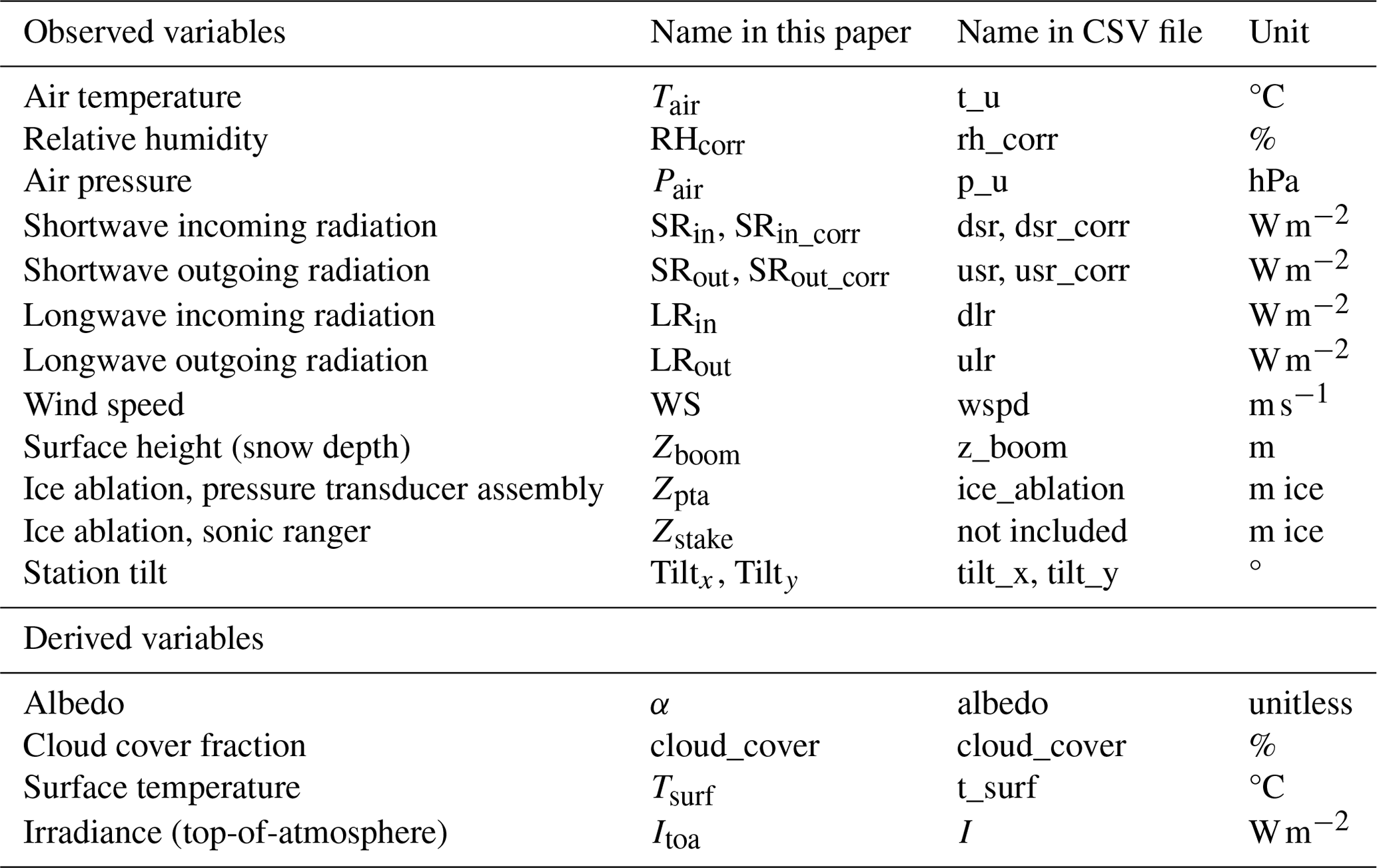
Table 3Instrument types and height above tripod feet and uncertainty and calibration schedule for the instruments installed at the three AAWSs on the A. P. Olsen transect. GEUS stands for Geological Survey of Denmark and Greenland.
3.1 Automatic ablation and weather station design
The AAWSs are designed as free-floating tripods (Fig. 2a) with instruments mounted on a top boom and on the mast (see Table 3 for a comprehensive list of instruments). These instruments maintain a fixed height above the tripod feet. In the ablation zone, this corresponds to the height above the surface during the melt season, when snow has completely melted away. During winter, as snow accumulates, the height of the instruments above the surface decreases (Fig. 2b). In the accumulation zone, where snow does not completely melt away each year, the instruments are manually lifted during field visits, causing the distance to the surface to vary throughout the year.
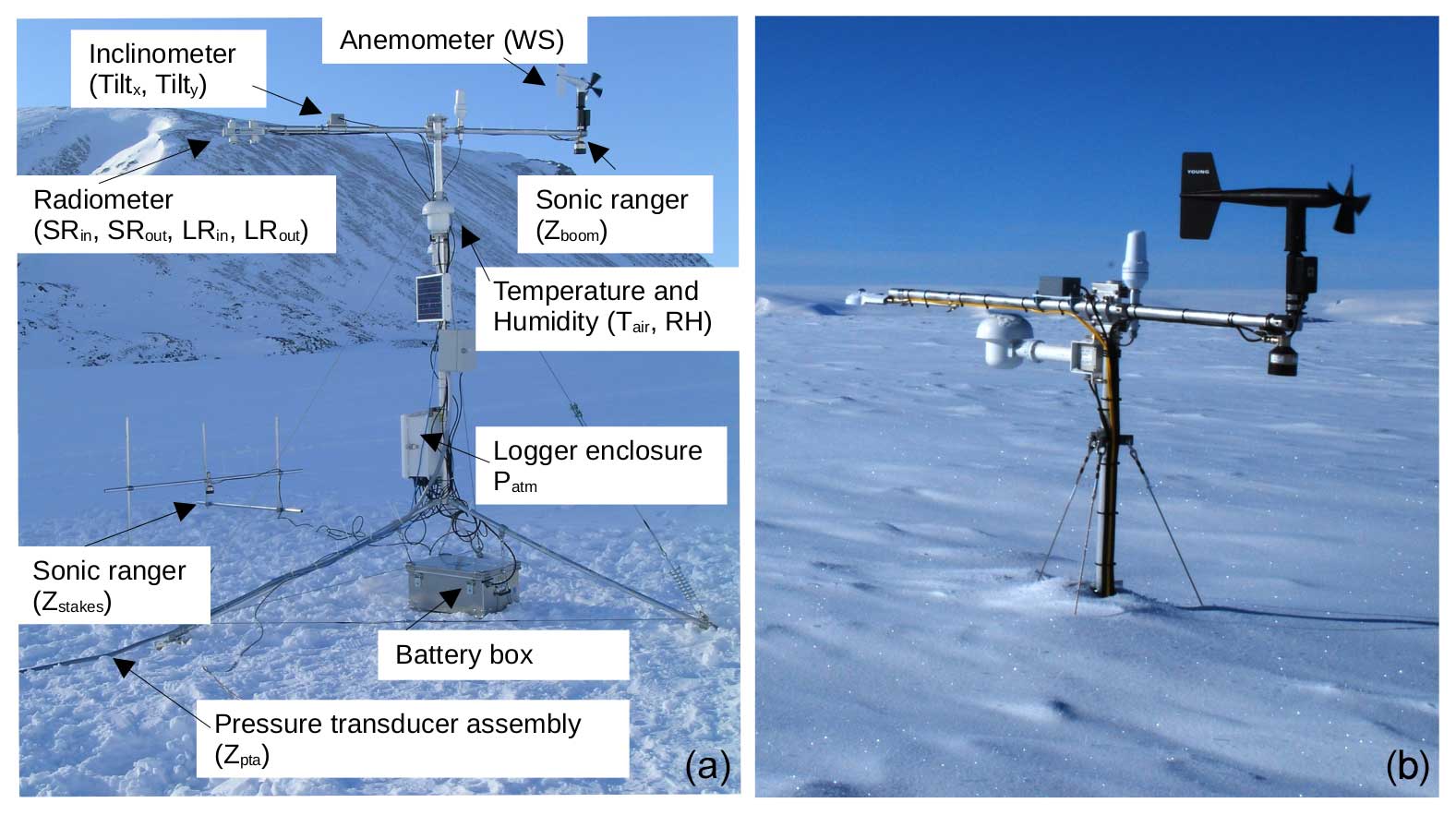
Figure 2(a) Photo of ZAC_L from installation in 2008, with labels showing the location of the instruments collecting the key variables published here. (b) Photo of ZAC_A from the field visit in April 2012 illustrating the gradual decrease in sensor height due to snow accumulation. Photo credit: Michele Citterio.
To conserve power, the data logger on the AAWS remains dormant and powers up at 10 min intervals to collect instantaneous values for all variables. The only exception is wind speed, which is measured by the number of propeller rotations since the last data collection. Therefore, the wind speed observation represents an average over the past 10 min.
3.1.1 Temperature and humidity
Air temperature (Tair) and relative humidity are measured using a sensor housed in a radiation shield equipped with a fan for forced ventilation. The ventilation is turned on 2 min prior to measurement to ensure a fully ventilated sensor. The instrument is placed at a height of approximately 2.6 m above the tripod feet. Temperature is measured with a PT100 sensor, and relative humidity is measured with a Rotronic HygroClip, which has a measurement uncertainty of ±0.8 %. The HygroClip is replaced with a freshly calibrated instrument at each field visit. It is recalibrated in a closed chamber at room temperature with constant relative humidity levels of 10 %, 35 %, and 80 %.
3.1.2 Radiation and station tilt
The four radiation components, incoming and outgoing short- and longwave radiation (SRin, SRout, LRin, and LRout) are measured using Kipp and Zonen CNR1 and CNR4 sensors, installed approximately 2.6 m above the tripod feet. According to the manufacturer, the measurement uncertainty is ±10 %. The instruments are replaced with newly calibrated ones every 4 years. The AAWS tripod floats freely on the ice surface in the ablation zone, causing both tilt and direction to vary as the surface melts. This movement particularly affects the recorded incoming and outgoing shortwave radiation. To correct for instrument tilt, the radiometer is accompanied by an inclinometer.
3.1.3 Air pressure
The air pressure Pair is measured with a Campbell Scientific CS100/Setra 2078 barometer placed inside the fiberglass-reinforced polyester logger enclosure located around 1.5 m from the tripod feet. A porous vent filter equalizes pressure inside and outside the logger enclosure. The measurement uncertainty in the instrument is reported to be 2 hPa in the range of −40 to 60 °C. The barometer has no fixed calibration schedule and has not been replaced at any of the stations.
3.1.4 Wind speed
Wind speed (WS) is measured with a R. M. Young anemometer model 05103-5. The anemometer is placed approximately 3 m above the tripod feet. The accuracy of the instrument is 0.3 m s−1 up to wind speeds of 30 m s−1, above which the accuracy is 1 %. The anemometer has no fixed calibration schedule and has only been replaced when broken by, for example, the tripod tipping over or being covered in snow.
3.1.5 Snow depth/sensor height
The distance between the surface and the instruments (Zboom), effectively measuring the snow height, is determined using a sonic ranger manufactured by Campbell Scientific (model SR50A) mounted on the AAWS boom. The sonic ranger measures the distance to the surface by recording the travel time of reflected sonic waves. According to Fausto and van As (2012), the instrument's accuracy ranges between 0.6 % and 0.7 % based on observations from the Greenland ice sheet, while the manufacturer reports an uncertainty of 0.4 %. The membrane of the sonic ranger is replaced every 1 to 2 years.
3.1.6 Ice ablation
Ice ablation is observed continuously, mainly using the pressure transducer assembly (PTA) described in detail in Fausto and van As (2012). The instrument consists of a pressure transducer installed at the end of a hose filled with antifreeze liquid. The pressure transducer measurement uncertainty is ±2.5 cm. The hose is drilled into the ice at a usual depth of 10 to 14 m. When the ice melts, the hose coils up on the surface and the liquid column pressure drops, and this drop in pressure is converted to surface-lowering Zpta. The PTA is replaced every approximately 3 years before melting out completely.
Supplementary to the pressure transducer assembly, a sonic ranger similar to the sensor measuring sensor height is mounted on separate stakes drilled into the ice.
3.2 Post-processing of data
After converting the observations to physical values using instrument calibration coefficients, the data are post-processed to remove observational artifacts, such as the effect of tilt on radiation observations and the temperature influence on sonic waves. As part of the post-processing, cloud cover and albedo are derived and included in the final dataset. After applying all corrections, hourly averages are calculated for hours where all six instantaneous observations are available.
3.2.1 Relative humidity
The relative humidity is measured relative to the maximum saturation of air and thus relative to liquid water, which, on glacier ice, is only valid at temperatures above freezing. For temperatures below the freezing point, the observed relative humidity (RHobs) is recalculated relative to ice using the method described in Goff and Gratch (1946):
where esice/water is the saturation water vapor pressure over ice or water. Relative humidity is filtered to contain only values between 0 % and 100 %.
The hourly average of relative humidity is calculated from averaging the vapor pressure (e) and then calculating back to relative humidity. The relation between vapor pressure and relative humidity is given by (based on Lowe, 1976)
where RH is relative humidity and es is specific humidity related to air temperature T via
See the given values for α0 to α6 in Appendix A.
3.2.2 Correction incoming shortwave radiation for tilt and deriving cloud cover
The tilt correction of incoming solar radiation follows van As (2011). Incoming shortwave radiation (SRin) can be split into a diffuse fraction (fdiff) and a direct fraction. The diffuse radiation is not affected by the tilt of the instrument, so it is only the direct beam part that is corrected:
where SZA is the solar zenith angle, d is the sun declination, w is the hour angle (see procedures for calculating SZA, d, and w in Iqbal (1983) or Reda and Andreas (2004)), lat is the instrument latitude in radians, and ϕsensor and θsensor are the tilt angle and direction, respectively.
The tilt-corrected values are passed through a filter removing spikes that exceed top-of-atmosphere irradiance given by
where I0=1361 W m−2 is the solar constant.
The diffuse fraction of the incoming shortwave radiation (fdiff) ranges from 0.2 to 1, corresponding to clear skies and fully overcast conditions, respectively, and we assume a linear relationship with the cloud cover fraction (cloud_cover).
The cloud cover fraction is calculated based on its dependence on air temperature (Tair) similar to the approach of van As et al. (2005). Firstly, the theoretical clear-sky incoming longwave radiation, LRclear, is calculated based on Swinbank (1963):
where T0=273.15 °C. Secondly, for theoretical overcast conditions, LRovercast, blackbody radiation is assumed:
The cloud cover fraction is thus:
And hence, the following applies:
The radiometer is repositioned towards south at every field visit. However, during the melt period, the station can change azimuth direction, and the exact direction of the instrument is not measured beyond the yearly field visits, which causes an uncertainty that is not quantified. This is addressed in the quality control in a later section.
3.2.3 Deriving albedo
The albedo is given by
and filtered to include only data when the sun is in view of the upper sensor, which is when the angle between the sun and the sensor (AngleDif) is below 70° and SZA is above 70°. AngleDif is given by
The gaps in the albedo record are filled using a forward fill function in order to use the albedo to correct the outgoing shortwave radiation as described below.
3.2.4 Correcting outgoing shortwave radiation
The radiation sensor has limitations when the sun angle is low and the sun beams hit the lower sensor intended to record outgoing shortwave radiation. When the sun is in the field of view of the outgoing sensor, it is assumed that the incoming sensor only records diffuse radiation. It is assumed that the sun is in view of the outgoing sensor when AngleDif below 90° and SZA is above 90°. The outgoing shortwave radiation is in this case calculated using the albedo:
3.2.5 Correcting snow depth/sensor height for temperature
The sonic wave speed in air depends on air temperature and thus the observed distances (Zboom_raw) are corrected for air temperature (Tair):
where T0=273.15 °C.
3.2.6 Correction of measured ice ablation
The pressure transducer assembly is an open system, and the ice ablation signal Zpta is therefore corrected for atmospheric pressure:
where PC is the calibration pressure provided by the manufacturer in hectopascals, Pair is the air pressure in hectopascals, g=9.81 m s−2 is the gravitational constant, and ρl is the density of the antifreeze liquid in the hose. The accuracy of the pressure transducer is 2.5 cm, and the standard deviation of the signal after the ice melt season has ended is 1.5 cm, with no systematical change relating to the depth of the sensor. For the purpose of making the data easy to use, the ice ablation observation is set to zero at the beginning of every melt season. This is done by subtracting the mean of a week prior to the onset of ice melt. The onset of ice melt is manually defined for each year by identifying the day when all three of the following conditions are met: albedo indicates ice (albedo values below 0.4); ice melt is detected in the pressure transducer assembly Zpta; and distance from the boom to the surface measured by the sonic ranger at the boom, Zboom, becomes constant. Since these observations are separate, determining the exact date is not always straightforward, and we estimate an uncertainty of up to ±2 d.
n the subsequent sections, we first detail major station failures, followed by an in-depth discussion on the quality and uncertainties associated with each specific variable. Our quality control process primarily involves a visual inspection of the data to identify outliers and detect data drift. Additionally, we compare variable gradients across the three AAWSs to identify periods with potentially problematic data. The success rate of our measurements after data filtering is depicted in Fig. 3. The unfiltered data could offer significant insights to expert users and are thus included as supplementary data in the dataset.
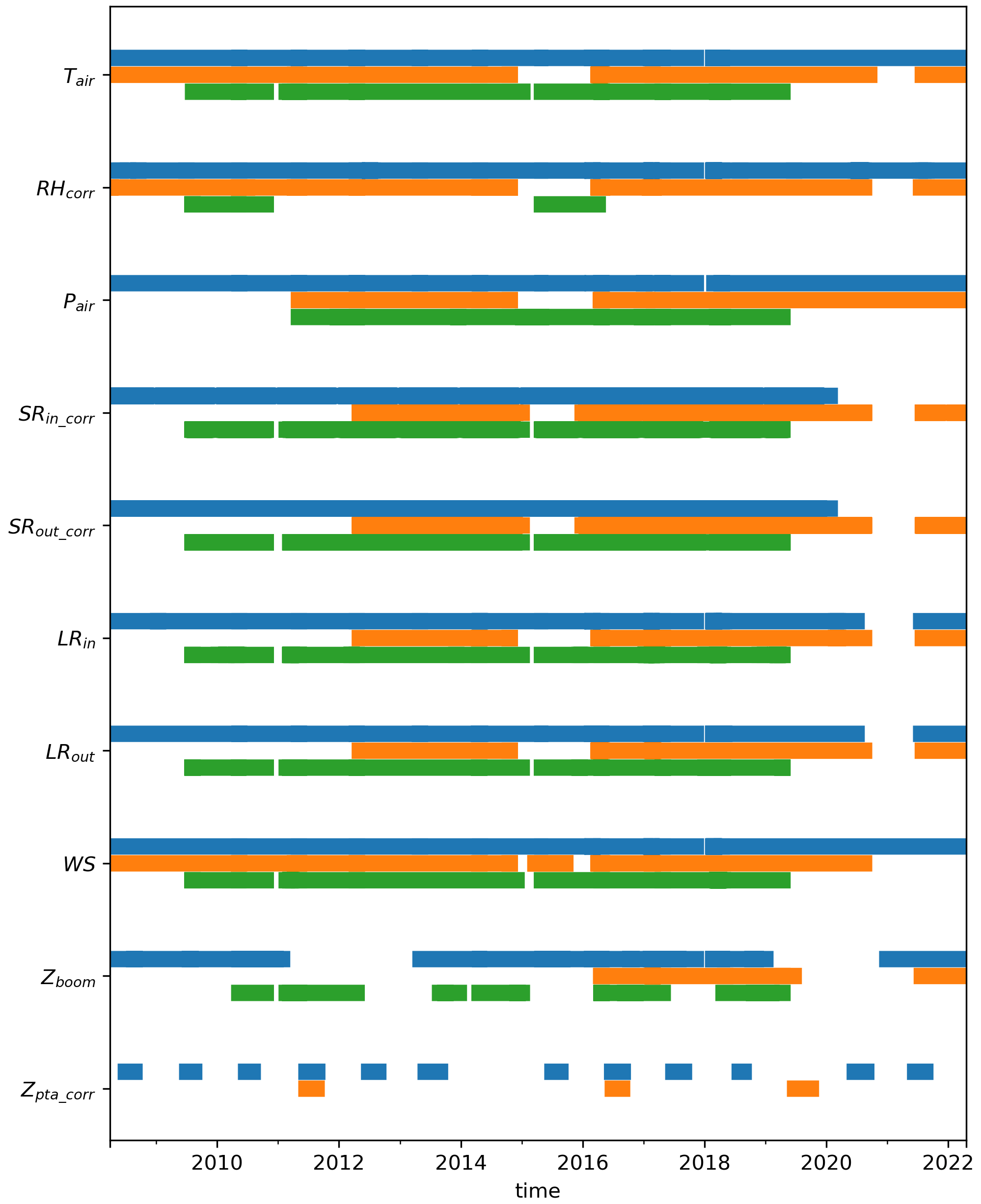
Figure 3Measurement success rate for the 10 key variables: blue is ZAC_L, orange is ZAC_U, and green in ZAC_A.
4.1 Major station failures
Reviewing the raw data and field notes, it becomes evident that several major events led to data loss across all variables, as described in the following.
In 2015, ZAC_U tipped over and was subsequently erected in April 2016. This incident is evident in the dataset as the data quality is poor, and data from all variables are removed for this period. ZAC_U tipped over again in 2020 and was erected and underwent repairs in July 2021. Data from this period have also been filtered out. During the winter of 2010/11, ZAC_A tilted or got snow-covered, and a part of the data was lost. In January 2015, most instruments at ZAC_A were buried by snow, only to be excavated in April 2015; these data are also filtered out. The ZAC_A record ends in April 2019, marking the final visit before the station was entirely buried in snow and could not be reached due to travel restrictions imposed during the COVID-19 pandemic.
4.2 Temperature
Temperature observations rely on the instrument casing being adequately ventilated. However, the ventilation fan consumes a significant amount of power and is deactivated when battery levels are low. This most often occurs during winter, when the batteries cannot be recharged due to the polar night. This coincides with the period when ventilation of the casing is less important, as the casing is not heated by shortwave radiation. Thus, we consider the effect to be minor and have not detected any problems with the data due to this.
To evaluate the data quality of temperature readings, we compare data year over year and examine the gradients in values between stations, as depicted in Fig. 4. This figure highlights the impact of the instrument burial at ZAC_A in 2015, which is evident from an unusual negative temperature gradient between ZAC_L and ZAC_A (see Fig. 4e). Additionally, the tilting incidents at ZAC_U in 2015 and 2020 manifest as unusually high and low lapse rates between ZAC_U and ZAC_L and ZAC_U and ZAC_A (see Fig. 4c and d). Aside from the major station problems, we found no quality issues with the air temperature observations.
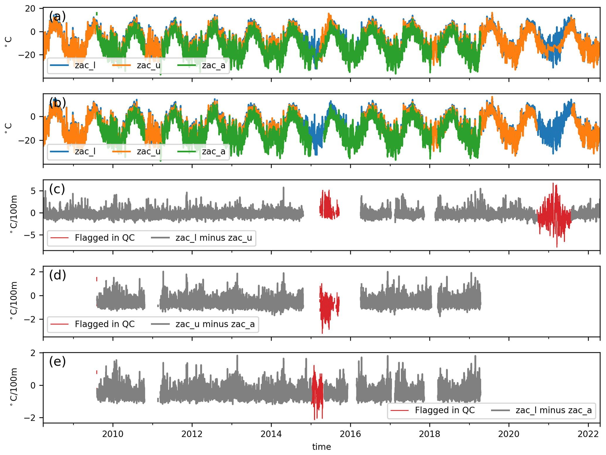
Figure 4Air temperature quality control. (a, b) Unfiltered and filtered data, respectively, ZAC_L is blue, ZAC_U is orange, and ZAC_A is green. (c) The temperature gradient per 100 m between ZAC_L and ZAC_U, ZAC_U and ZAC_A, and ZAC_L and ZAC_A, respectively. The gray line indicates data considered to show natural variation, and the red line denotes flagged data considered to show variability caused by a faulty sensor at one of the stations.
4.3 Relative humidity
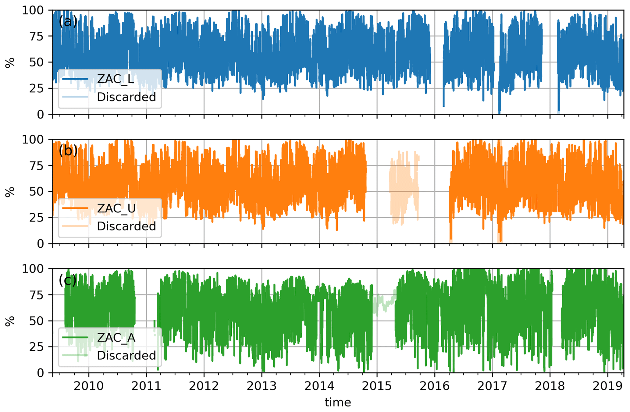
The humidity sensor typically requires recalibration every 1–2 years. However, due to logistical challenges, this was not always feasible, and an uncalibrated sensor will drift towards increasingly poorer performance. Drifting values of relative humidity are hard to objectively quantify. From a visual inspection of the relative humidity time series in Fig. 5, drifting could have occurred at ZAC_A during 2012–2014, but we will leave it up to the user to define when data are useful.
4.4 Shortwave radiation and tilt
The radiation sensor can be affected by shorter periods, with riming causing outliers, which is partly dealt with by removing outliers beyond fixed thresholds as described for the individual variables. The radiation sensors also face issues related to high tilt and azimuth misalignment from the south; we assumed that the effect of this on the longwave radiation component is negligible, but tilt can have a significant effect on the shortwave component. During each field visit, the AAWS is adjusted to ensure the radiometer faces south. However, as the AAWS floats on the surface, it can tilt as well as rotate at varying degrees during the melt season. While the shortwave radiation is corrected for tilt, the correction does not take azimuth misalignment into account. If the sensor turns more towards the west or east, the tilt correction can become inaccurate as it operates under the assumption that the sensor is oriented southward. The uncertainty in the tilt-corrected shortwave radiation can be evaluated by investigating the total tilt, the size of the correction, by comparing SRin_corr with SRin as well as the corrected values to potential incoming radiation as done in the following.
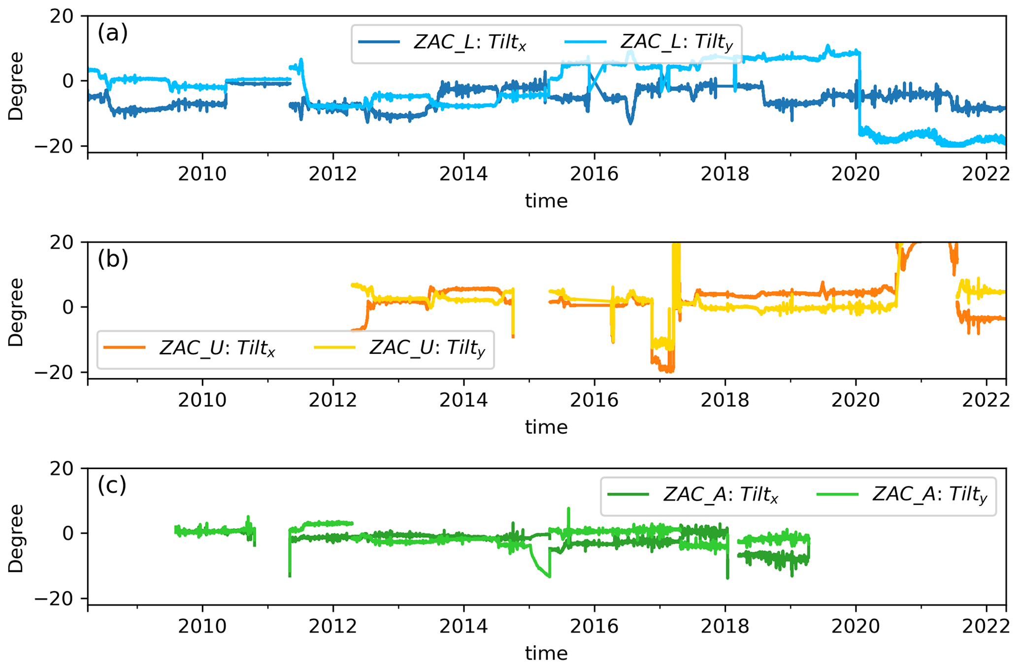
Figure 6 displays the x and y components of the measured tilt. Typically, the AAWS tilt does not exceed an absolute value of 10°. Exceptions to this are instances when a station has been entirely tipped over or buried in snow. The tilt varies the most at ZAC_L, which is in line with observations of a very uneven surface during field visits. ZAC_A is more stable due to its position in the accumulation zone, where it is stabilized by the snow. In January 2020, a shift in Tilty at ZAC_L occurred. Field notes indicate this was caused by damage to the tripod legs and subsequent loosening of the guy-wires after the station was covered with snow.
The tilt-corrected incoming shortwave radiation is shown in Fig. 7. The peak values of the data vary significantly at ZAC_L. While this could be due to natural variations as ZAC_L is located low in a valley prone to low clouds, it might also be due to poor data quality. To evaluate the success of the tilt correction and the quality of or uncertainty in the radiation data, we compare corrected and non-corrected shortwave incoming radiation in Fig. 8. The top-of-atmosphere irradiance (Itoa, Eq. 6) is used as a visual guideline, with the shaded gray area showing the span of Itoa over 1 d.
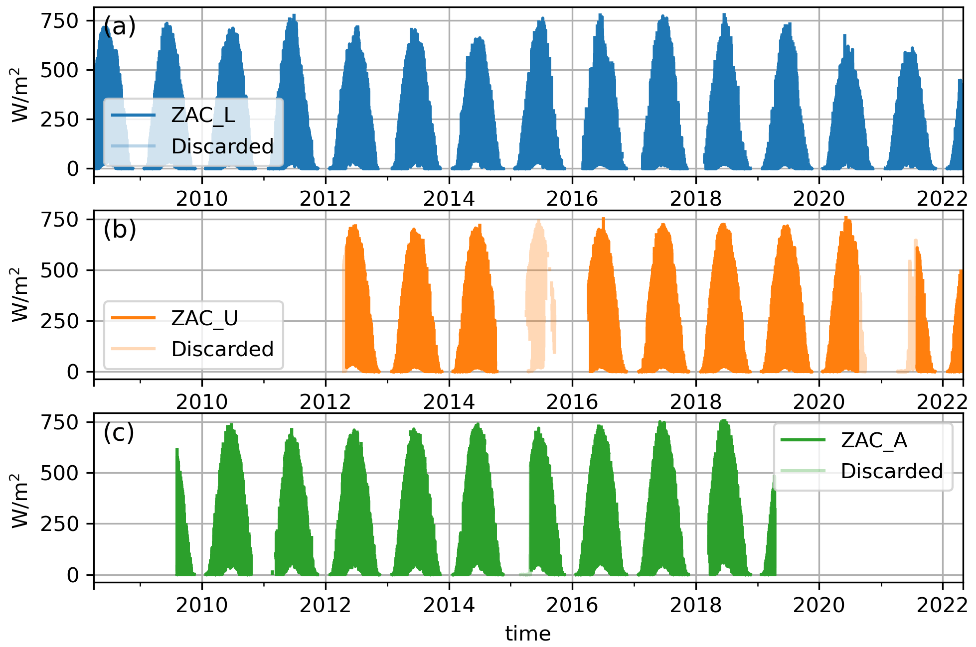
Figure 7Incoming shortwave radiation corrected for tilt (SRin_corr) at ZAC_L (a), ZAC_U (b), and ZAC_A (c).
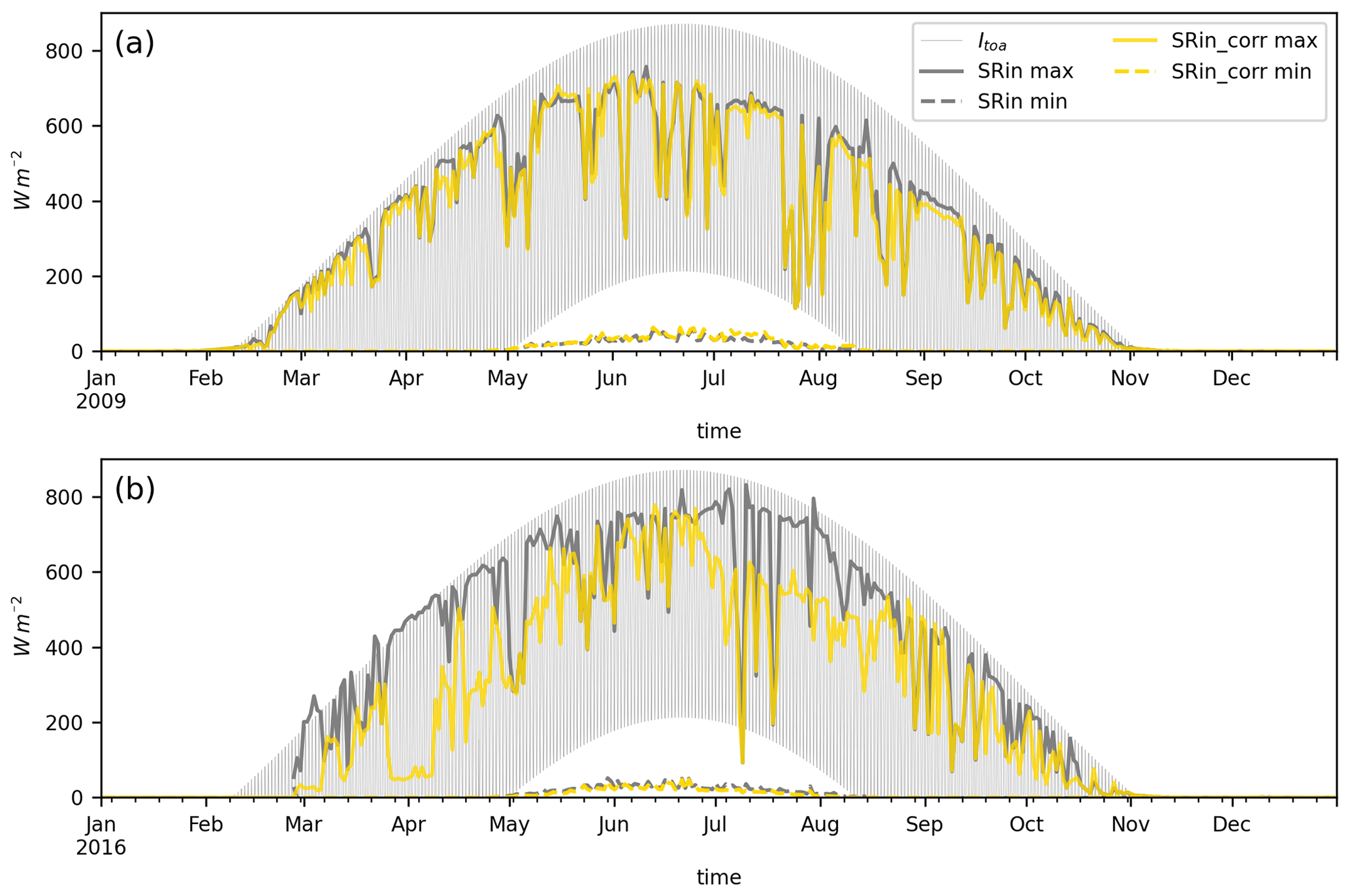
Figure 8Assessment of the effect of tilt correction in 2009 (a) and 2016 (b) at ZAC_L: the shaded gray area spans the daily calculated maximum and minimum top-of-atmosphere incoming shortwave radiation (see Eq. 6). The solid lines represents the daily maximum observed incoming shortwave radiation before (gray) and after (yellow) the tilt correction. Similarly, the dashed lines represent the daily minimum observed radiation before (gray) and after (yellow) the tilt correction.
Panel (a) in Fig. 8, with data from ZAC_L in 2009, shows a successful year where the tilt correction modifies the values slightly. Panel (b) in Fig. 8 shows a year where the tilt of the station was more severe, indicating higher uncertainties in such years. Specifically, at ZAC_L, incoming shortwave radiation from the years spanning 2012 to 2016 and 2018 to 2020 needed more correction than in other years, and uncertainty in SRin is expected to be higher for these years. Figure 8 also shows that the minimum values of observed SRin range well below the minimum Itoa. This discrepancy is due to the shading of the station – particularly during summer nights, when the sun angle is low and coming from the north.
Finally, the quality of incoming and outgoing shortwave radiation is evaluated in comparison with remotely sensed albedo values. The albedo values used are from the Google Earth Engine AlbedoInspector (https://www.glacier-hub.com/posts/GEE-toolbox-for-glacier/, last access: 9 September 2024) based on the work done by Feng et al. (2023) in Fig. 9. The comparison between a point measurement from the AAWS with a grid value introduces an uncertainty. There is a generally good correlation between the in situ and remotely sensed albedo values with a goodness of fit, R2, of 0.55, which is comparable to the values obtained by Feng et al. (2023) when comparing the satellite-derived albedo with PROMICE data.
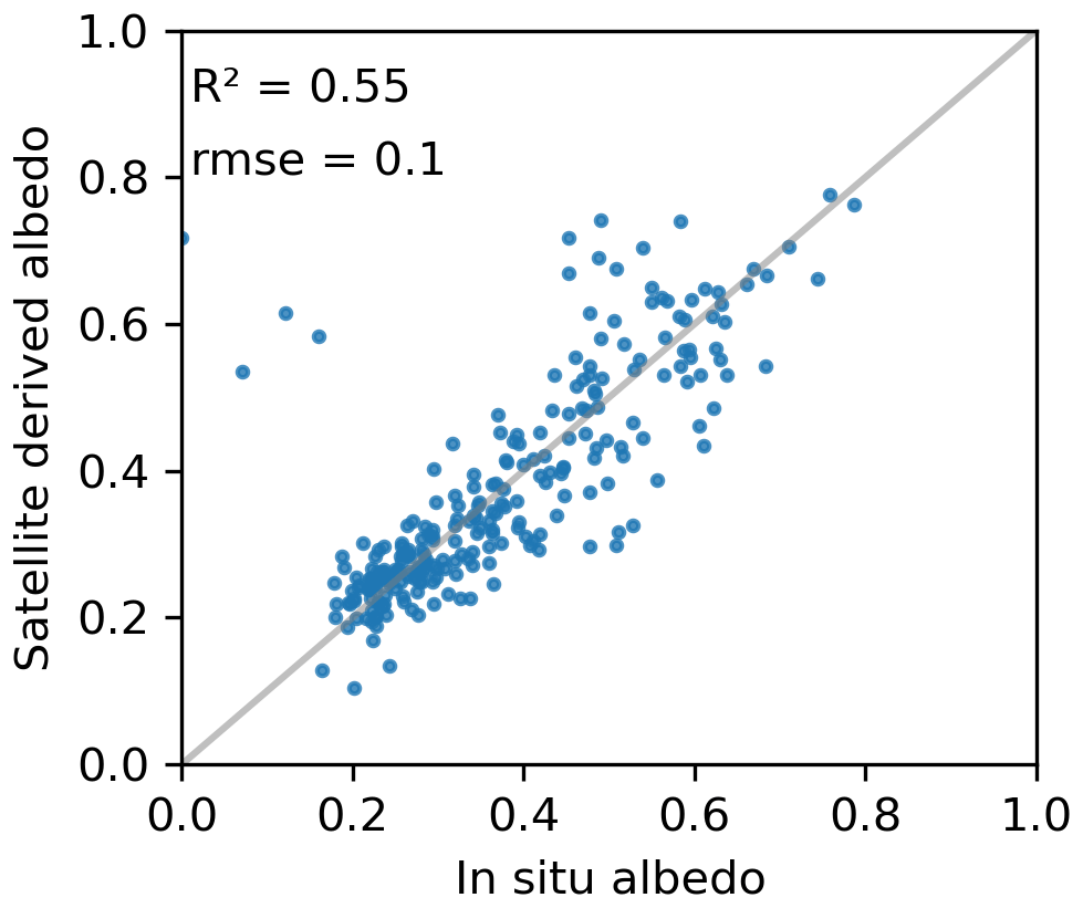
Figure 9Daily albedo values: in situ observations compared with the satellite-derived ones based on Feng et al. (2023).
4.5 Longwave incoming and outgoing radiation
The incoming and outgoing longwave radiation shows some instances of outliers of unusually low values. We believe these events are caused by riming events. The most extreme cases are filtered out by excluding all incoming longwave radiation data (LRin) lower than 120 W m−2 and all outgoing longwave radiation (LRout) lower than 150 W m−2 (Fig. 10).
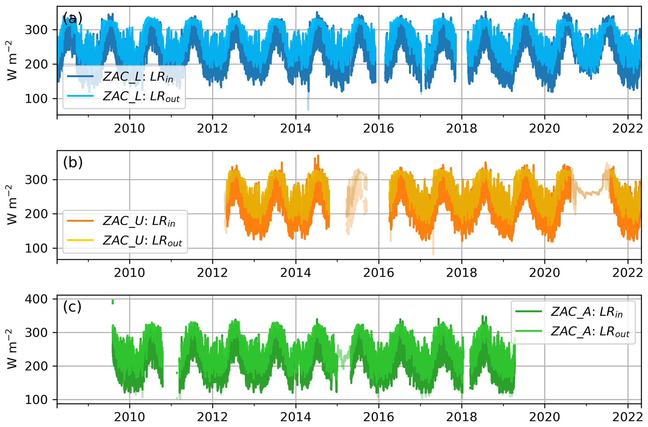
Figure 10Incoming and outgoing longwave radiation (LRin, LRout) at (a) ZAC_L, (b) ZAC_U, and (c) ZAC_A. Pale colors indicate data that have been filtered out.
There is a period between July 2020 and July 2021 at ZAC_L where the longwave radiation data look substantially higher than in the rest of the period. The cause of this remains elusive, and the data are filtered out.
4.6 Air pressure and wind speed
We saw no quality issues with air pressure and wind speed data, and only data from the periods where the stations have either tipped over or got buried in snow have been filtered out from the air pressure and wind speed data. The air pressure is dependent on absolute elevation of the stations, and the elevation values given in this paper are based on a multi-year average of a single-frequency GPS on the AAWS.
4.7 Ice ablation
The PTA only records ice melt, and the presence of snow cover over the instrument can influence the data. Consequently, all data from October to March are automatically discarded. Instances when the pressure transducer assembly completely melted out of the ice have also been removed, meaning not every year contains a complete melt season. To assess data quality, we compare the ice ablation observations from the PTA (Zpta) with those from the sonic ranger on stakes (Zstake). This comparison is limited to ZAC_L since ice ablation has only been measured by a PTA at ZAC_U and ZAC_A is situated in the accumulation zone.
Overlapping ice ablation data from ZAC_L span 6 years, as shown in Fig. 11. In 2008 and 2009, the PTA recorded faster ice ablation rates than the sonic ranger. Notably, according to field notes, in July 2009, the stake assembly holding the sonic ranger collapsed. This incident with a tilting stake assembly might be the cause of the lower melt rates observed by the sonic ranger. In 2010, the stake assembly was re-established, while the PTA setup remained unchanged, and the sonic ranger recorded higher melt rates than the PTA. This indicates no consistent undercatch in the PTA system. The PTA melted away in 2010 and did not capture the late part of the melt season. In 2012, the melt rates of the two systems were similar until late July. For 2015 and 2016, the melt rates of the two systems were closely aligned. However, by the end of the 2016 melt season, the two curves diverge. This variation could be due to a snowfall event visible in the sonic ranger data but not in the PTA. Differences between the two datasets could also arise if they represent distinct surface areas with varying darkness or turbulence conditions.
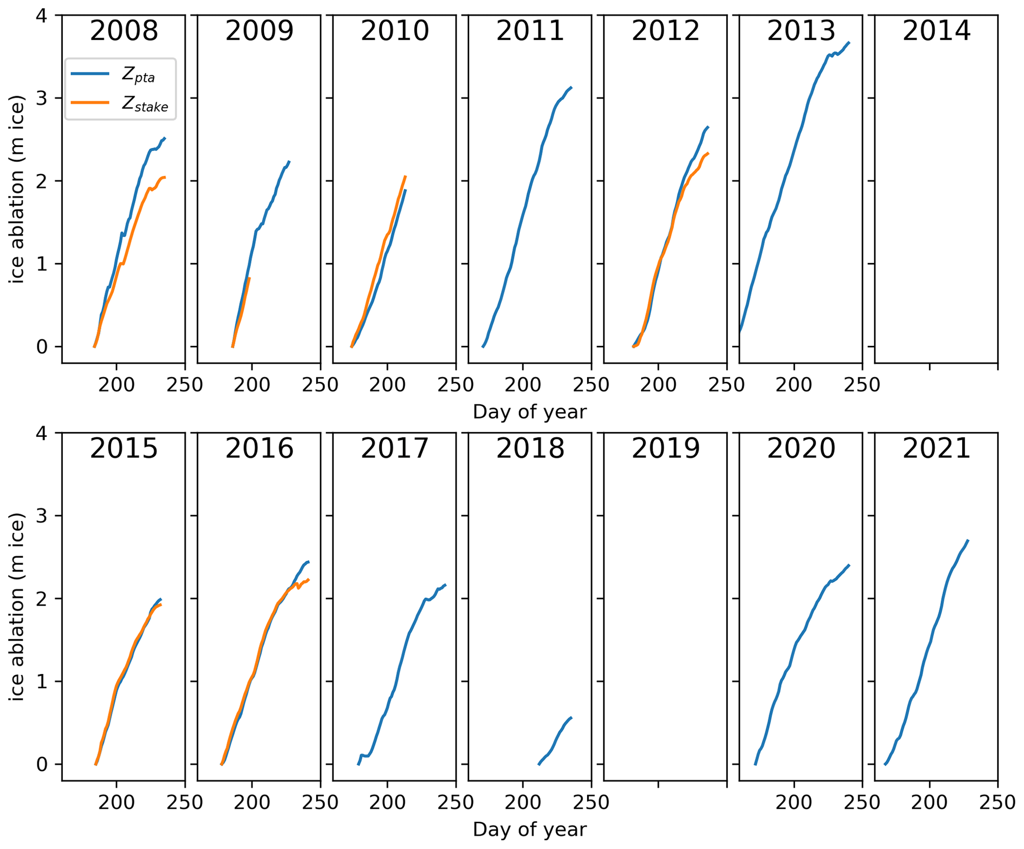
Figure 11Ice ablation recorded using the pressure transducer assembly (blue) and the sonic ranger on stakes (orange) at ZAC_L. Subplots with no data are years where both instruments failed.
Generally, we trust the ice ablation data from the PTA (Zpta) more than the sonic ranger observations (Zstake). However, discrepancies between the two, as seen in 2012 and 2016, illustrate the uncertainty in the ice ablation observations. Snowfall events during the ice melt season are not captured by the PTA. This should be kept in mind when using the data for evaluating, for example, an energy balance model as seen below.
The variables collected at the A. P. Olsen transect are key variables in the surface energy budget equations and can be used for calculating the energy availability for melting ice. In this use case, we exemplify how a point energy budget melt model can be set up using the observed variables. The energy budget model is implemented at ZAC_L and depends on the observed radiation budget (SRin_corr, SRout_corr, LRin, and LRout), temperature (Tair), wind speed (WS), air pressure (Pair), and relative humidity (RHcorr). The use case focuses on 2 years, 2009 and 2016, when the tilt correction on the radiation data was, respectively, low and high.
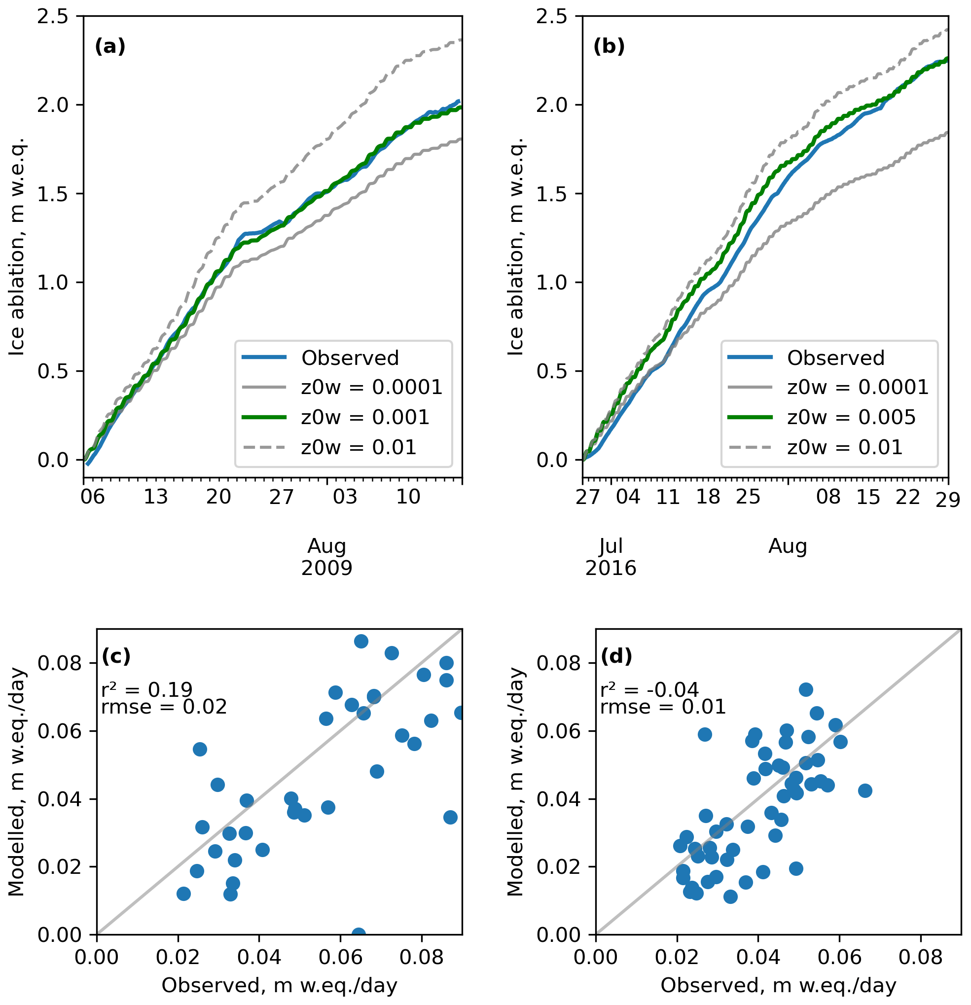
Figure 12Results from the energy budget ice melt model. (a, b) Accumulated modeled melt compared with observed ice melt for 2009 and 2016, respectively. (c, d) Daily modeled ice melt compared with observed daily ice ablation from Zpta_corr for 2009 and 2016, respectively.
The energy budget is the balance between the net shortwave radiation, ; the net longwave radiation, ; and the turbulent heat fluxes – latent heat flux, Hl, and sensible heat flux, Hs, as well as the ground heat flux, G. Thus, the energy available for melt is given by
For the purpose of this example, we neglect G, assuming the contribution from this is minor compared to the contribution from other sources, as in Abermann et al. (2019). The turbulent heat fluxes are calculated following Monin–Obukhov theory (as done in Hock and Noetzli, 1997), where the following applies:
Also, the following applies:
where e2 is the vapor pressure at instrument level given by the Clausius–Clapeyron relation, written as
and e0 is the vapor pressure at a melting surface; cp is the specific heat of dry air; L is the latent heat of sublimation when e2−e0 is negative and the latent heat of evaporation when e2−e0 is positive and equal to zero; κ=0.41 is the von Kármán constant; ρ0 is the air density at the mean atmospheric level, P0; z is the instrument height, assumed here to be constant, at 2.7 m; z0w, z0t, and z0e are the roughness lengths for logarithmic profiles of wind, temperature, and water vapor, respectively. z0w is kept as a calibration constant and can be varied, while z0t and z0e are assumed to be 100 times smaller than z0w. All three roughness lengths could be varied to calibrate the model, but this is out of the scope of this example.
The energy surplus is converted to melt by dividing with the latent heat of fusion (Lf=334 000 J kg−1) so that
This is only valid for a melting surface.
The point melt is calibrated by varying the surface roughness factor for wind, z0w, within the range between 0.01 and 0.0001 as this value has been shown to vary with orders of magnitude (e.g., Smeets and Broeke, 2008). All the uncertainties introduced by the two model assumptions are in this way summarized in this single static value. For the purposes of this example, we define a successful calibration on a seasonal scale, thus choosing the value of z0w that gives a total melt over a melt season that best matches the total observed ablation over the same season (Fig. 12a and b). Model performance is then evaluated on a daily timescale by accumulating the modeled melt to daily sums and comparing these to the observed daily melt rates (Fig. 12b and c). The observed melt rates are calculated as the difference between the minimum and the maximum value of the Zpta_corr over 1 d. A value of z0w=0.001 was found to match the 2009 total ablation, while z0w=0.005 was more appropriate for 2016. The performance of the melt model on a daily scale is affected by both model assumptions and observational uncertainty in both variables used to calculate the energy available for melt as well as the validation data. We suspect that the high tilt of the AAWS in 2016 could explain the lower R2 value in this year compared to 2009.
The dataset can be found at https://doi.org/10.22008/FK2/X9X9GN (Larsen and Citterio, 2023) and in the GEM database at https://data.g-e-m.dk/ (last access: 9 September 2024). Future refinements will be uploaded as new versions, and the continuation of the transect time series is available via https://doi.org/10.22008/FK2/IW73UU (How et al., 2022). Please note that due to a discrepancy in the definitions of glacier catchments, ZAC_L and ZAC_U are in the east catchment (RGI ID RGI60-05.20098), but ZAC_A is attributed to RGI ID RGI60-05.20092, labeled the north catchment in Fig. 1.
The data processing code, taking the data from raw to usable data, is provided as documentation and can be found on GitHub at https://GitHub.com/GEUS-Glaciology-and-Climate/GlacioBasis_AWS_processing (last access: 12 September 2024) and Zenodo (https://doi.org/10.5281/zenodo.13736151, Larsen, 2024a). The point energy budget model script can be found at https://GitHub.com/GEUS-Glaciology-and-Climate/GlacioBasis_essd_point_energy_balance_model (last access: 12 September 2024) and Zenodo (https://doi.org/10.5281/zenodo.13736164, Larsen, 2024b).
This paper presented the near-surface climate and ice ablation dataset from a transect of three automatic weather and ablation stations on the A. P. Olsen Ice Cap in northeast Greenland, for the period from 2008 through May 2022. The dataset contains key components needed to calculate the surface energy balance: ice ablation, air temperature, relative humidity, air pressure, wind speed, and incoming and outgoing longwave radiation, as well as the derived variables of cloud cover fraction and albedo. The dataset has gone through rigorous instrument corrections and quality control. It can be used to study surface energy budget and ablation processes and to force, calibrate, or validate distributed models. Despite the rigorous quality control, uncertainties remain; the most important for the energy budget calculations are uncertainties in the shortwave radiation and the observed ice ablation. The dataset is a unique transect of near-surface climate on a local ice cap in Greenland and constitutes the first 15 years of a continuous glaciological monitoring effort in northeast Greenland as part of the Greenland Ecosystem Monitoring program.
The constants used in Eq. (3) are
SHL led the writing of the paper and transformed the data from raw measurements into the published format, in some parts utilizing the open-source code from the PROMICE workflow. MC had designed the monitoring program as project manager from 2007 to 2021 and collected most of the data, with great help from the other co-authors. DB, BH, and AR contributed with the collection and correction of data. RSF helped with utilizing the knowledge from the PROMICE data workflow. All co-authors have contributed to writing the paper.
The contact author has declared that none of the authors has any competing interests.
Publisher's note: Copernicus Publications remains neutral with regard to jurisdictional claims made in the text, published maps, institutional affiliations, or any other geographical representation in this paper. While Copernicus Publications makes every effort to include appropriate place names, the final responsibility lies with the authors.
This work was supported by the Greenland Ecosystem Monitoring program (https://g-e-m.dk/, last access: 9 September 2024) via the sub-program GlacioBasis. GlacioBasis would not exist if not for Andreas Peter Ahlstrøms's initiative with the first application. We thank Zackenberg Research Station for support. Many people have helped conduct the fieldwork; in particular, we thank the GeoBasis sub-program for support in the field as well as field participants through the years – namely, Horst Machguth, Ylva Sjöberg, Morten Langer Andersen, Cristina Gerli, and Marek Stibal. The design and maintenance of the A. P. Olsen transect are not possible without the support from the GlacioLab at the Geological Survey of Denmark and Greenland (GEUS), where the design, development, and building of certain instruments take place in close collaboration with PROMICE and GC-Net. Some errors in the raw data were discovered as part of the collaboration with Sonika Shahi at University of Graz, who meticulously went through the data during the quality control process.
This research has been supported by the Danish Energy Agency (Climate and Environmental Support).
This paper was edited by Achim A. Beylich and reviewed by three anonymous referees.
Abermann, J., As, D. V., Wacker, S., Langley, K., Machguth, H., and Fausto, R. S.: Strong contrast in mass and energy balance between a coastal mountain glacier and the Greenland ice sheet, J. Glaciol., 65, 263–269, https://doi.org/10.1017/jog.2019.4, 2019. a, b
Bolch, T., Sørensen, L. S., Simonsen, S. B., Mölg, N., MacHguth, H., Rastner, P., and Paul, F.: Mass loss of Greenland's glaciers and ice caps 2003–2008 revealed from ICESat laser altimetry data, Geophys. Res. Lett., 40, 875–881, https://doi.org/10.1002/grl.50270, 2013. a
Citterio, M., Sejr, M. K., Langen, P. L., Mottram, R. H., Abermann, J., Larsen, S. H., Skov, K., and Lund, M.: Towards quantifying the glacial runoff signal in the freshwater input to Tyrolerfjord–Young Sound, NE Greenland, Ambio, 46, 146–159, https://doi.org/10.1007/s13280-016-0876-4, 2017. a
Fausto, R. S. and van As, D.: Ablation observations for 2008–2011 from the Programme for Monitoring of the Greenland Ice Sheet (PROMICE), Geological Survey of Denmark and Greenland, GEUS Bulletin, 26, 73–76, 2012. a, b
Fausto, R. S., van As, D., Mankoff, K. D., Vandecrux, B., Citterio, M., Ahlstrøm, A. P., Andersen, S. B., Colgan, W., Karlsson, N. B., Kjeldsen, K. K., Korsgaard, N. J., Larsen, S. H., Nielsen, S., Pedersen, A. Ø., Shields, C. L., Solgaard, A. M., and Box, J. E.: Programme for Monitoring of the Greenland Ice Sheet (PROMICE) automatic weather station data, Earth Syst. Sci. Data, 13, 3819–3845, https://doi.org/10.5194/essd-13-3819-2021, 2021. a, b
Feng, S., Cook, J. M., Anesio, A. M., Benning, L. G., and Tranter, M.: Long time series (1984–2020) of albedo variations on the Greenland ice sheet from harmonized Landsat and Sentinel 2 imagery, J. Glaciol., 6, 1225–1240, https://doi.org/10.1017/jog.2023.11, 2023. a, b, c
Goff, J. A. and Gratch, S.: Low-pressure properties of water-from 160 to 212 °F, Trans. Am. Heat. Vent. Eng., 52, 95–121, 1946. a
Hock, R. and Holmgren, B.: A distributed surface energy-balance model for complex topography and its application to Storglaciären, Sweden, J. Glaciol., 51, 25–36, https://doi.org/10.3189/172756505781829566, 2005. a
Hock, R. and Noetzli, C.: Areal melt and discharge modelling of Storglaciären, Sweden, Ann. Glaciol., 24, 211–216, 1997. a
How, P., Abermann, J., Ahlstrøm, A., Andersen, S., Box, J. E., Citterio, M., Colgan, W., Fausto, R., Karlsson, N., Jakobsen, J., Langley, K., Larsen, S., Mankoff, K., Pedersen, A., Rutishauser, A., Shield, C., Solgaard, A., van As, D., Vandecrux, B., and Wright, P.: PROMICE and GC-Net automated weather station data in Greenland, V11, GEUS Dataverse [data set], https://doi.org/10.22008/FK2/IW73UU, 2022. a
How, P. R., Wright, P. J., Mankoff, K. D., Vandecrux, B., Fausto, R. S., and Ahlstrøm, A. P.: pypromice: A Python package for processing automated weather station data, Journal of Open Source Software, 8, 5298, https://doi.org/10.21105/joss.05298, 2023. a, b
Hugonnet, R., McNabb, R., Berthier, E., Menounos, B., Nuth, C., Girod, L., Farinotti, D., Huss, M., Dussaillant, I., Brun, F., and Kääb, A.: Accelerated global glacier mass loss in the early twenty-first century, Nature, 592, 726–731, https://doi.org/10.1038/s41586-021-03436-z, 2021. a
Iqbal, M.: An Introduction to Solar Radiation, Academic Press, ISBN 978-0-12-373750-2, https://doi.org/10.1016/B978-0-12-373750-2.X5001-0, 1983. a
Khan, S. A., Colgan, W., Neumann, T. A., van den Broeke, M. R., Brunt, K. M., Noël, B., Bamber, J. L., Hassan, J., and Bjørk, A. A.: Accelerating Ice Loss From Peripheral Glaciers in North Greenland, Geophys. Res. Lett., 49, e2022GL098915, https://doi.org/10.1029/2022GL098915, 2022. a
Larsen, S. H.: GEUS-Glaciology-and-Climate/GlacioBasis_AWS_processing: Code release for ESSD manuscript (essd_paper), Zenodo [code], https://doi.org/10.5281/zenodo.13736151, 2024a. a
Larsen, S. H.: GEUS-Glaciology-and-Climate/GlacioBasis_essd_point_energy_balance_model: Code release for ESSD manuscript (essd_paper), Zenodo [code], https://doi.org/10.5281/zenodo.13736164, 2024b. a
Larsen, S. H. and Citterio, M.: GlacioBasis Zackenberg – Level 1 data 2008–2022, GEUS Dataverse, V1, https://doi.org/10.22008/FK2/X9X9GN, 2023. a, b
Lowe, P. R.: An Approximation Polynomial for the Computation of Saturation Vapor Pressure, J. Appl. Meteorol., 16, 100–103, 1976. a
Lund, M., Stiegler, C., Abermann, J., Citterio, M., Hansen, B. U., and van As, D.: Spatiotemporal variability in surface energy balance across tundra, snow and ice in Greenland, Ambio, 46, 81–93, https://doi.org/10.1007/s13280-016-0867-5, 2017. a
Machguth, H., Rastner, P., Bolch, T., Mölg, N., Sørensen, L. S., Aalgeirsdottir, G., Angelen, J. H. V., Broeke, M. R. V. D., and Fettweis, X.: The future sea-level rise contribution of Greenland's glaciers and ice caps, Environ. Res. Lett., 8, 025005, https://doi.org/10.1088/1748-9326/8/2/025005, 2013. a
Noël, B., Berg, W. J. V. D., Lhermitte, S., Wouters, B., Machguth, H., Howat, I., Citterio, M., Moholdt, G., Lenaerts, J. T., and Broeke, M. R. V. D.: A tipping point in refreezing accelerates mass loss of Greenland's glaciers and ice caps, Nat. Commun., 8, 14730, https://doi.org/10.1038/ncomms14730, 2017. a
Reda, I. and Andreas, A.: Solar position algorithm for solar radiation applications, Sol. Energy, 76, 577–589, https://doi.org/10.1016/j.solener.2003.12.003, 2004. a
RGI Consortium: Randolph Glacier Inventory – A Dataset of Global Glacier Outlines, Version 6. Greenland Periphery subset, Boulder, Colorado USA, NSIDC: National Snow and Ice Data Center, https://doi.org/10.7265/4m1f-gd79, 2017. a, b
Sauter, T., Arndt, A., and Schneider, C.: COSIPY v1.3 – an open-source coupled snowpack and ice surface energy and mass balance model, Geosci. Model Dev., 13, 5645–5662, https://doi.org/10.5194/gmd-13-5645-2020, 2020. a
Sejr, M. K., Bruhn, A., Dalsgaard, T., Juul-Pedersen, T., Stedmon, C. A., Blicher, M., Meire, L., Mankoff, K. D., and Thyrring, J.: Glacial meltwater determines the balance between autotrophic and heterotrophic processes in a Greenland fjord, P. Natl. Acad. Sci. USA, 119, e2207024119, https://doi.org/10.1073/pnas.2207024119, 2022. a
Shahi, S., Abermann, J., Silva, T., Langley, K., Larsen, S. H., Mastepanov, M., and Schöner, W.: The importance of regional sea-ice variability for the coastal climate and near-surface temperature gradients in Northeast Greenland, Weather Clim. Dynam., 4, 747–771, https://doi.org/10.5194/wcd-4-747-2023, 2023. a
Smeets, C. J. and Broeke, M. R.: Temporal and spatial variations of the aerodynamic roughness length in the ablation zone of the greenland ice sheet, Bound.-Lay. Meteorol., 128, 315–338, https://doi.org/10.1007/s10546-008-9291-0, 2008. a
Swinbank, W. C.: Long-wave radiation from clear skies, Q. J. Roy. Meteor. Soc., 89, 339–348, 1963. a
van As, D.: Warming, glacier melt and surface energy budget from weather station observations in the melville bay region of northwest greenland, J. Glaciol., 57, 208–220, https://doi.org/10.3189/002214311796405898, 2011. a
van As, D., van den Broeke, M., Reijmer, C., and van de Wal, R.: The summer surface energy balance of the high Antarctic plateau, Bound.-Lay. Meteorol., 115, 289–317, https://doi.org/10.1007/s10546-004-4631-1, 2005. a
Vandecrux, B., Box, J. E., Ahlstrøm, A. P., Andersen, S. B., Bayou, N., Colgan, W. T., Cullen, N. J., Fausto, R. S., Haas-Artho, D., Heilig, A., Houtz, D. A., How, P., Iosifescu Enescu, I., Karlsson, N. B., Kurup Buchholz, R., Mankoff, K. D., McGrath, D., Molotch, N. P., Perren, B., Revheim, M. K., Rutishauser, A., Sampson, K., Schneebeli, M., Starkweather, S., Steffen, S., Weber, J., Wright, P. J., Zwally, H. J., and Steffen, K.: The historical Greenland Climate Network (GC-Net) curated and augmented level-1 dataset, Earth Syst. Sci. Data, 15, 5467–5489, https://doi.org/10.5194/essd-15-5467-2023, 2023. a
- Abstract
- Introduction
- Study area and monitoring setup
- Instruments and methodology
- Data quality, uncertainty, and filtering
- Use case – a point energy budget melt model
- Code and data availability
- Conclusions
- Appendix A
- Author contributions
- Competing interests
- Disclaimer
- Acknowledgements
- Financial support
- Review statement
- References