the Creative Commons Attribution 4.0 License.
the Creative Commons Attribution 4.0 License.
 | 12 Sep 2024
A database of deep convective systems derived from the intercalibrated meteorological geostationary satellite fleet and the TOOCAN algorithm (2012–2020)
Rémy Roca
We introduce two databases, TOOCAN (Tracking Of Organized Convection Algorithm using a 3D segmentatioN) and CACATOES, aimed at facilitating the study of deep convective systems (DCSs) and their morphological characteristics over the intertropical belt during the period spanning from 2012 to 2020. The TOOCAN database is constructed using a tracking algorithm called TOOCAN applied on a homogenized GEOring infrared (IR) archive and enables the documentation of the morphological parameters of each DCS throughout their life cycles. The homogenized GEOring IR database has been built from level-1 data of a fleet of geostationary platforms originating from various sources and has been intercalibrated; spectrally adjusted; and limb-darkening corrected, specifically for high cold clouds, based on a common reference, the IR channel of the Scanner for Radiation Budget (ScaRaB) radiometer on board the Megha-Tropiques. The resulting infrared observations are then homogeneous for brightness temperatures (BT) <240 K, with a standard deviation lower than 1.5 K, throughout the GEOring. A systematic uncertainty analysis is carried out. First, the radiometric errors are shown to have little impact on the DCS characteristics and occurrences. We further evaluate the impact of missing data and demonstrate that a maximum of 3 h of consecutive missing images represents a favorable compromise for maintaining tracking continuity while minimizing the impact on the DCS morphological parameters. However, beyond this temporal threshold, the segmentation of DCS is significantly compromised, necessitating the interruption of the tracking process. The CACATOES database is derived from the TOOCAN database through a post-processing procedure, which involves projecting the morphological parameters of each deep convective system (DCS) onto a daily 1° × 1° grid. The resultant dataset provides a broader perspective, allowing for an Eulerian analysis of the DCS and facilitating comparisons with auxiliary gridded datasets on the same daily 1° × 1° grid box.
Both the TOOCAN and CACATOES databases are provided in a common netCDF format that is compliant with the standards of Climate and Forecast (CF) conventions and the Attribute Convention for Dataset Discovery (ACDD).
A total of 15×106 DCSs have been identified over the tropical regions and the 9-year period. The analysis of DCSs over the tropical oceans and continents reveals a large variety of DCS characteristics and organizations. They can last from few hours up to several days, and their cloud shield ranges from 1000 km2 to a few millions of squared kilometers. Oceanic DCSs are characterized by a longer lifetime duration and larger shields. Finally, the DCS geographical distribution is in line with previous DCS climatologies built from other algorithms and satellite observations.
All datasets can be accessed via the repository under the following data DOIs:
-
TOOCAN database: https://doi.org/10.14768/1be7fd53-8b81-416e-90d5-002b36b30cf8 (Fiolleau and Roca, 2023a)
-
CACATOES database: https://doi.org/10.14768/98569eea-d056-412d-9f52-73ea07b9cdca (Fiolleau and Roca, 2023b).
- Article
(7682 KB) - Full-text XML
- BibTeX
- EndNote


Deep convective systems (DCSs) are central to the hydrological and energy cycles of the tropical region (Roca et al., 2014, 2010). Despite a long research history (Houze, 2018), understanding the lifetime duration of tropical convective systems and the lengths of their various phases throughout their life cycles in the current climate, as well as their evolution in a warmer and moister world, remains challenging (Roca et al., 2020). Deep convective systems in the tropics can span a wide range of scales (10–1000 km) and degrees of organization (Houze, 2004). Within this full spectrum of organized convection, mesoscale convective systems (MCSs) form a specific family of deep convective systems producing contiguous precipitation on horizontal scales larger than 100 km (Houze, 2004) and which can organize into mesoscale convective complexes (Maddox, 1980), squall-line systems, and super clusters (Mapes and Houze, 1993). DCSs are composed of a convective core where heavy rainfall takes place, associated with a stratiform anvil with lighter precipitation, as well as non-precipitating cirriform cloudiness. DCSs are further characterized by a life cycle. DCSs initiate and develop from one or more individual deep convective cells, which organize themselves into convective cores. The system then enters a maturity phase in which a stratiform part and cirriform cloud expand. Finally, as convection vanishes, DCSs are no longer fed by convective cells; they dissipate and scatter into several individual cirriform clouds.
Well-curated global satellite observations can provide a useful resource to constraint theoretical and modeling perspectives on deep convective systems. In particular, after decades of field campaigns and detailed case studies, satellite climatology can now support the statistical analysis needed to refine our current understanding. Indeed, the information related to the life cycle of deep convective systems can only be obtained statistically at the tropical scale by using high-frequency imagery available from the geostationary orbit. Meteorological agencies around the world have successfully operated geostationary satellites for more than 4 decades.
From the 1980s, and in the context of campaign measurements (GATE, WMOMEX, etc.), some automatic tracking algorithms have been developed and implemented for the detection and tracking of convective systems from infrared (IR) imagery of geostationary satellites. Tracking algorithms are generally based on two steps: a detection step to identify contiguous areas of cold temperatures in a single IR image, referred to as cloud clusters in which deep convection is organized, and a tracking step to match the identified cloud clusters from one frame to the next. Over the course of its life cycle, a deep convective system corresponds to a succession of cloud clusters in a time sequence of IR images. Tracking algorithms have evolved over time, in line with the ways in which we describe deep convective systems, with the improvements in geostationary imagers and with the technical advances allowing an improvement in the identification and tracking of deep convective systems and their high cold-cloud shields.
The detection stage is historically based on the thresholding of the IR images using brightness temperature (BT) thresholds to delineate the cloud clusters. In the literature, a wide range of temperature thresholds – from 208 to 253 K – have been used to detect cloud clusters at different degrees of organization. Hence, Williams and Houze (1987) identified cloud clusters larger than 5000 km2 with a 213 K threshold, while Maddox (1980) applied a 241 K threshold to identify the high cold-cloud shield associated with mesoscale convective complexes (MCCs) over the central United States. Machado et al. (1992) studied the dependence of cloud cluster size on the choice of brightness temperature threshold for different tropical regions. They found that temperature thresholds in the range of 240–255 K had little effect on the surface of the cloud clusters. Over the years, developments have been made in terms of the detection stages, and these have improved the characterization of cloud clusters. Thus, Mathon and Laurent (2001) identified cloud clusters larger than 5000 km2 by applying three different temperature thresholds to the infrared imagery: a 213 K temperature threshold to discriminate deep convective cores; a 233 K threshold commonly used to estimate surface precipitation in the tropics (Arkin, 1979); and a 253 K threshold to identify the boundaries of the high cold-cloud shield. In this way, it is possible to access the number of convective cores included in a high cloud shield. This technique has been adopted by Evans and Shemo (1996) and Ocasio et al. (2020), with some slightly different brightness temperature thresholds.
However, detection steps based on single brightness temperature thresholds face some difficulties with regard to catching the complexity of the full spectrum of convective organization (Fiolleau and Roca, 2013a). A single BT threshold tends to identify cloud cover but cannot differentiate the components that make up convective systems. To improve the high cold-cloud segmentation, Boer and Ramanathan (1997) have developed an algorithm called Detect And Spread (DAS). It relies on the assumption that pixels adjacent to a convective core in an IR satellite image belong to the same physical cloud cluster and that the optical depth of cloud cover decreases from the convective core to the edge of the cloud cluster. The algorithm is based on a region-growing technique consisting of the application of multiple brightness temperature thresholds to the IR images in order to identify the convective cores, which are then spread to reach the boundaries of the cloud shield. Similar approaches have been adopted by Roca and Ramanathan (2000), Feng et al. (2021), Heikenfeld et al. (2019), Wilcox (2003), Rajagopal et al. (2023), and Autones and Moisselin (2013).
Regarding the tracking step, Williams and Houze (1987) introduced the area-overlapping technique to link cloud clusters in successive images, building the convective systems from their initiation to their dissipations. This technique has been widely used for years (Arnaud et al., 1992; Mathon and Laurent, 2001; Machado et al., 1998) and has been the subject of numerous technical evolutions to increase the matching accuracy between clusters identified in two successive time steps. Hence, to enhance the cloud matching, the projection of the cloud position has been added in some tracking methods (Ocasio et al., 2020; Feng et al., 2023). Huang et al. (2018) combined a Kalman filter technique with the area-overlapping method to improve the tracking of small and fast-moving convective systems. Some algorithms have based their tracking stages on a search radius method and on the prediction of the position of the cloud cluster's center of mass to link cloud clusters to each other (Heikenfeld et al., 2019; Woodley et al., 1980; Ostlund, 1974). Carvalho and Jones (2001) and Endlich and Wolf (1981) used the maximum spatial correlation between cloud clusters of successive images, while Hodges (1994) developed a minimization of cost function to improve the cloud cluster correspondence issue between two time steps.
However, tracking algorithms based on the two-step technique (detection step and tracking step) can result in artificial splitting and merging artifacts throughout DCS life cycles that require specific post-processing (Feng et al., 2021; Williams and Houze, 1987; Mathon and Laurent, 2001); these remain a major source of uncertainty when considering DCS life cycle analysis (Prein et al., 2024).
To overcome these issues, another branch of algorithms has been developed based on the assumption that convective systems can only be tracked if they are considered to be three-dimensional (space + time) objects in their space–time domain. These algorithms no longer work on the basis of IR image per IR image but process a volume of IR images in three dimensions (longitude, latitude, time) to identify and track convective systems in a single step. Some algorithms then apply a single brightness temperature threshold in the spatio-temporal domain to detect and track deep convective systems (Mapes et al., 2009; Dias et al., 2012; Prein et al., 2024; Poujol et al., 2020). Other tracking algorithms use a more complex technique and apply a 3D multi-step, multi-thresholding technique, derived from the Detect-and-Spread method (Boer and Ramanathan, 1997), to the volume of IR imagery (Fiolleau and Roca, 2013a; Jones et al., 2023). With such a 3D segmentation technique, high cold cloudiness is decomposed in deep convective systems which are not impacted by splitting and merging events, as for previous tracking algorithms. At the beginning of the DCS life cycle, the individual convective cells which develop are part of the same DCS and feed its anvil. Similarly, at the end of the DCS life cycle, the scattered cirriform clouds all belong to the same DCS which produced them.
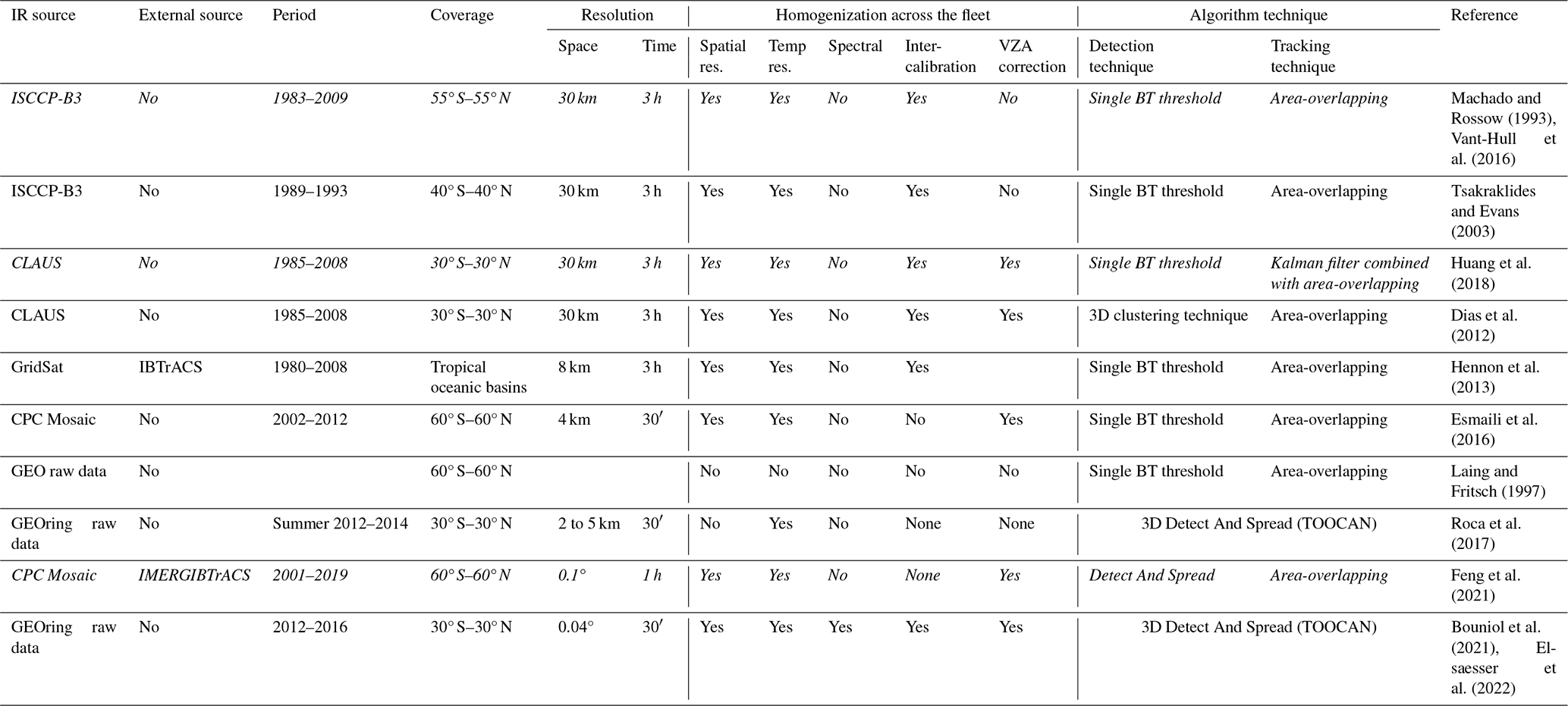
These tracking algorithms have given rise to a large corpus of literature at the regional scale, but only a few databases of deep convective systems have been made available at the global scale so far based on various global infrared archives (Table 1). These climatologies provided an initial perspective at the tropical scale, revealing the ubiquity of mesoscale systems with various durations and spatial extents across a wide spectrum of large-scale environments. This insight has prompted numerous scientific investigations. For instance, Elsaesser et al. (2022) investigated the growth rate of the cloud shield across the entire tropical belt. Using the CLAUS dataset, the statistics of DCS triggering revealed the strong link to orography, while spectral analysis brought about observational support to theories of tropical dynamics (Dias et al., 2012). The overwhelming contribution of the long-lasting systems to the total tropical-precipitation amount was quantitatively estimated (Roca et al., 2014), along with that to the extreme precipitation (Roca and Fiolleau, 2020). The recent decades' tropical trends in precipitation have been shown to be associated with the trends in the occurrence of deep organized systems (Tan et al., 2015). These examples constitute a strong incentive to build and sustain IR-derived databases of the DCS morphology in support of climatological investigations of the tropical water cycle (Feng et al., 2021).
Table 1Technical characteristics of the existing DCS databases over the entire tropical band. The DCS databases made available and associated with a DOI are indicated in italic.
On the other hand, the limitations of the IR information in documenting the precipitating processes occurring at the sub-storm scale are well known (Liu et al., 2007), yet the IR-based convective cloud shield analysis can provide significant insights into the dynamics of the system. A simple two-stage model can describe well the life cycle of the DCS shield and can show that the morphological parameters of the storms are so tightly related that, eventually, the full life cycle of the cloud shield can be reconstructed knowing, for instance, only the duration and the maximum extension of the system (Roca et al., 2017). IR-derived information about the DCS life is crucial to contextualize overpassing observations, be it active or passive microwave observations (Fiolleau and Roca, 2013b; Bouniol et al., 2016). The knowledge of the cloud shield can further inform physically based precipitation retrievals (Bellerby et al., 2009; Guilloteau and Foufoula-Georgiou, 2024). Such a variety of applications is one more strong motivation to elaborate upon the infrared archive to document the life cycle of DCSs in support of process studies.
Cloud-tracking algorithms further add requirements to the GEOring1 dataset used to elaborate upon global mesoscale convective system (MCS) climatology. While a few studies rely on 3-hourly data, it is important to make use of at least 30 min imagery to describe the full spectrum of deep convective systems (Fiolleau and Roca, 2013a). Similarly, high-resolution observations are required to address the full life cycle of the convective systems that could otherwise be truncated (Schröder et al., 2009). The variety of spatial and spectral resolutions, for instance, for the period 2012–2020 (see discussion below) further calls for a homogenization effort at the first level prior to running the tracking algorithm (Fiolleau et al., 2020).
This paper presents such a DCS database built from a homogenized IR archive and a tracking algorithm called TOOCAN (Tracking Of Organized Convection Algorithm using a 3D segmentatioN) (Fiolleau and Roca, 2013a). In Sect. 2, we present the harmonized infrared geostationary dataset and the way we have performed the homogenization procedure using the Scanner for Radiation Budget (ScaRaB) (on board the Megha-Tropiques) IR observations. We will then introduce the International Best Track Archive for Climate Stewardship (IBTrACS) dataset, which will be used to filter out DCSs belonging to a cyclonic circulation or DCSs that are themselves classified as cyclonic events. The functioning of the TOOCAN algorithm is introduced in Sect. 3. We will discuss the possible uncertainty in the deep-convective-system occurrences and characteristics induced by the residual error of the homogenization procedure, as well as the geostationary data availability. Exemplary illustrations of the database are shown in Sect. 4, and, finally, the data availability and format are further discussed in Sect. 5.
2.1 The harmonized infrared geostationary dataset for 2012–2020
Thermal-channel brightness temperature data obtained by the operational meteorological geostationary satellite fleet are used to monitor the deep convective systems over the tropical belt for the whole 2012–2020 period. Table 2 shows the technical characteristics of the fleet of geostationary platforms (GEOring) and their associated IR channels over the 9-year period. As shown in Fiolleau et al. (2020), the GEOring is far from a homogeneous suite of instruments operated in similar fashion. Spatial and temporal resolutions, as well as the spectral-filter functions and the calibration procedures, differ from one platform to another. All of these technical differences lead to biases in the brightness temperature measurement from one geostationary platform to another. To overcome such issues, Fiolleau et al. (2020) developed a methodology for the homogenization of the thermal infrared channels of the meteorological geostationary satellite fleet for cold-cloud studies based on the IR channel of the Scanner for Radiation Budget (ScaRaB) on board the Megha-Tropiques. This homogenization procedure includes the computation of the intercalibration and spectral normalization coefficients every 10 d, as well as the correction of the limb-darkening effects impacting the brightness temperature measurements from geostationary satellites in the range of 180–240 K for the 2012–2016 period. The extension of the geostationary database until 2020 has required us to continue this harmonization effort. These 4 additional years are characterized by the launch of new geostationary satellites. Over the Indian Ocean, METEOSAT-7 was replaced by MSG-1 in January 2017, and the new-generation GOES-16 replaced GOES-13 over the Americas in December 2017. Finally, over the eastern Pacific region, the GOES-15 platform was shifted from its initial nadir at 135° W to 128° W in November 2017 to ensure continuity of observations in the eastern Pacific before being replaced by GOES-17 in December 2019. From the end of 2018, the Megha-Tropiques satellite has suffered from technical issues in the data management subsystem, implying a decrease in the availability of the ScaRaB data. From this date, only about 30 % of the data are available. Nevertheless, the quality of the ScaRaB measurements is not impacted by such technical issues, and ScaRaB has shown the same performance as at the beginning of the mission. To overcome the lack of ScaRaB observations, the calculation of intercalibration and spectral-normalization coefficients was carried out every 30 d instead of the initial 10 d.
Table 2Technical characteristics of the operational geostationary satellite fleet and the associated imagers used over the 2012–2020 period.
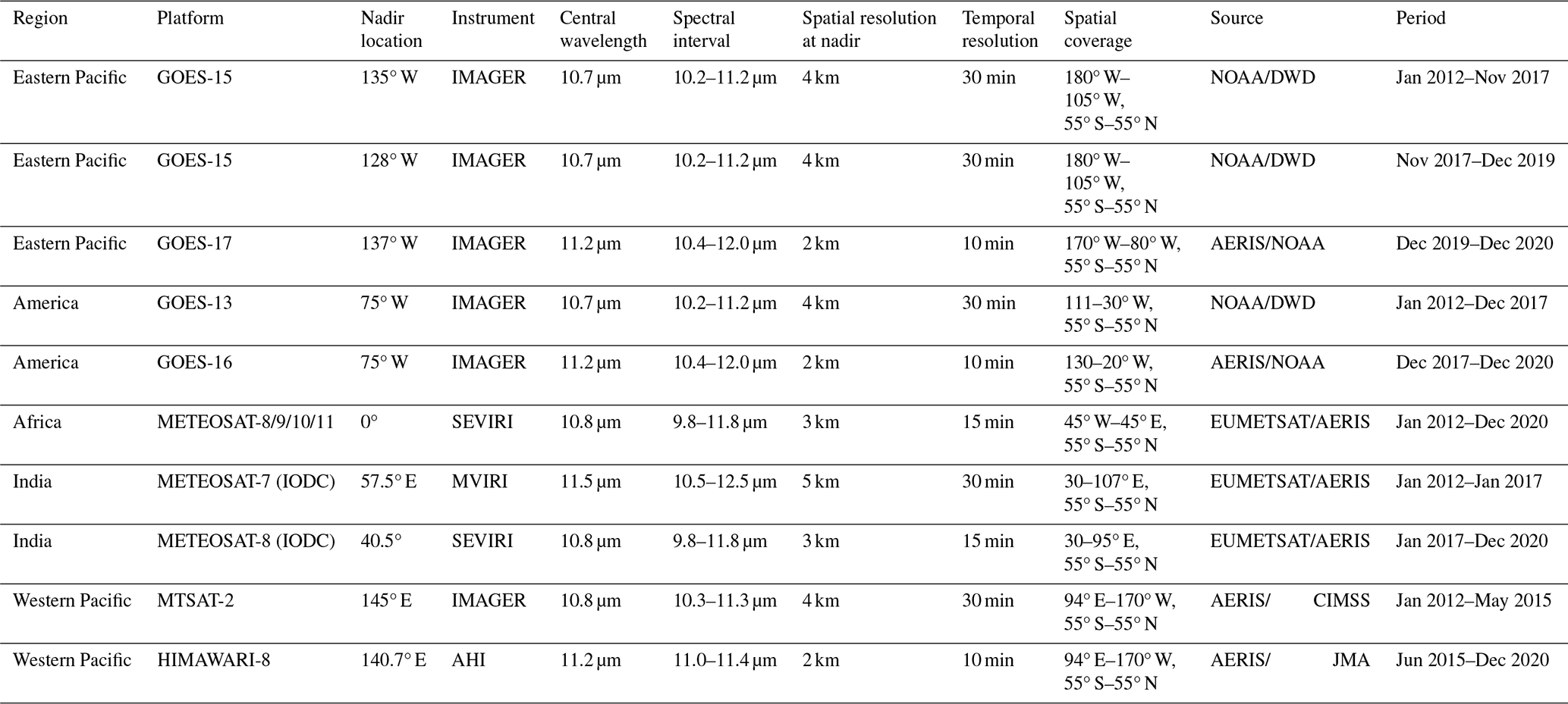
Figure 1a shows the time series of the initial bias in BT for all the geostationary imagers with respect to the ScaRaB observation in the range 180–240 K and for geostationary zenith angles lower than 20° over the 2012–2020 period. The large bias observed in the MET7/MVIRI calibration between 2012 and 2017 (Fig. 1a) is explained by significant ice contamination on the MVIRI optics, as fully discussed in Hewison et al. (2013) and Fiolleau et al. (2020). The results of the intercalibration and spectral normalization are shown Fig. 1b. Over the entire period and for all the geostationary platforms, the decadal residual bias indicates a very small and stable bias (<0.04 K), with a standard deviation lower than 0.07 K, between BTSCARAB and the intercalibrated BTGEO (BTGEO*). The decrease in the ScaRaB data availability does not impact the quality of the corrections from the end of 2018. The limb-darkening correction is the final step of the harmonization process and is performed on the basis of geostationary satellite per geostationary satellite. The method has been fully described in Fiolleau et al. (2020). Figure 2 shows the variation in the biases of BTGEO* for values lower than 235 K between pairs of geostationary satellites monitoring the same region according to the difference in their zenith angles (ΔVZA) before and after zenith angle corrections. Without any corrections, BTGEO* bias varies from −5 to +5 K as the ΔVZA moves from −50 to 50° regardless of the geostationary platform (Fig. 2a). By applying the zenith angle correction, this bias averages 0.21 K, with a standard deviation of 1.33 K, throughout the GEOring independently of the variation in ΔVZA.
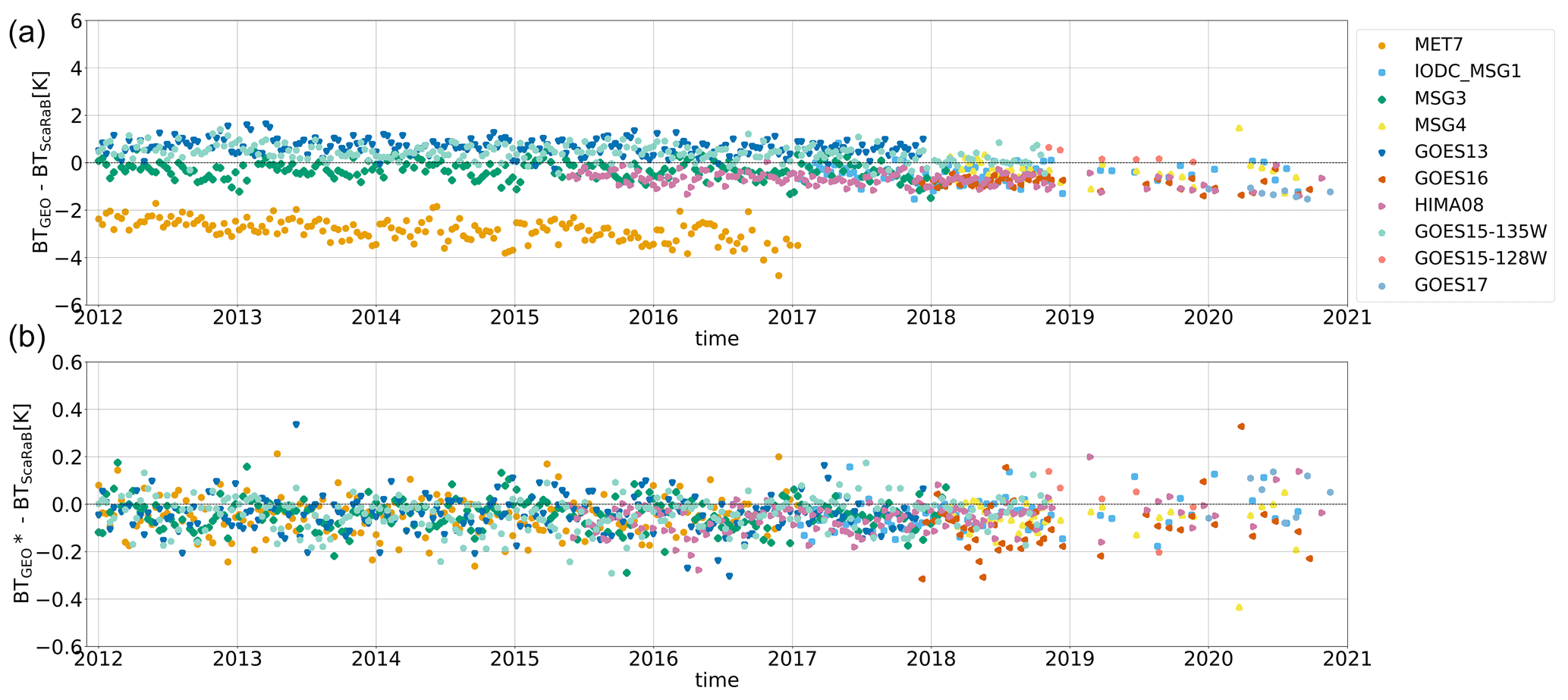
Figure 1(a) Time series of initial BT bias in geostationary IR observations with respect to SCARAB in the range 180–240 K between 2012 and 2020; (b) after spectral and calibration corrections.
To finalize the harmonization procedure, the temporal resolution has been unified to 30 min across the GEOring, and all the geostationary data have been remapped into a common longitude–latitude 0.04° equal-angle grid (Fiolleau et al., 2020). The spatial coverage of each geostationary satellite has been chosen to be relatively wide in longitude in order to have an important overlapping area between adjacent geostationary platforms and between 55° S and 55° N in latitude.
GOES-13 and GOES-15 sensors follow a complex sector-scanning schedule. The full disk images are produced every 3 h, while the Northern Hemisphere and the Southern Hemisphere images are produced every 30 min with a time lag of a few minutes between each scan. Thus, to get a full disk image at a 30 min temporal resolution, the southern and northern scans of GOES-13 and GOES-15 have been concatenated. The acquisition schemes of the MTSAT-1 and MTSAT-2 platforms (from January 2012 to May 2015) over the western Pacific region only provide Northern Hemisphere imagery at a 30 min frequency; that of the Southern Hemisphere zone is only available every hour. Similarly, a small region of the Southern Hemisphere between 118 and 108° W is only monitored at a 3 h temporal resolution by GOES-15.
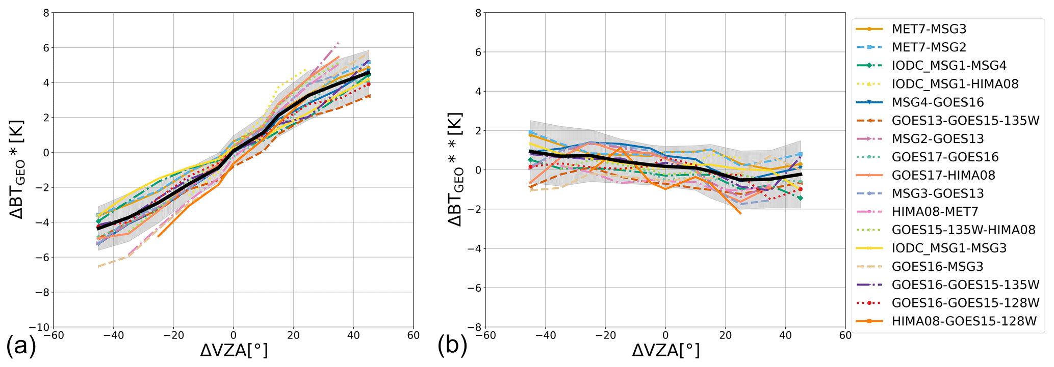
Figure 2(a) Variation of the BT bias according to the VZA differences between pairs of geostationary platforms observing common areas and for BTSCARAB in the range 180–235 K between 2012 and 2020 before viewing-zenith-angle corrections; (b) after viewing-zenith-angle corrections. The BT bias and its standard deviation for all the pairs of geostationary platforms are represented, respectively, by the black line and the gray-filled area.
Low-quality infrared images have been filtered out by applying a quality control on all the geostationary IR data (Szantai et al., 2011). Overall, the availability of all the geostationary platforms during the 2012–2020 period exceeds 96.8 %, with the highest availability over Africa (99.6 %) and the lowest availability over the western Pacific region (95 %). Figure 3 shows the time series of the missing data for all the geostationary platforms. METEOSAT-7 over India is impacted during the boreal summer by solar eclipses, and data are not disseminated for a couple of hours each day from early August to mid-September and from February to March. We can notice that the replacement of METEOSAT-7 by MSG-1 in January 2017 drastically increases the data availability. Similarly, the time series highlight the improvement in data availability as the configuration of the fleet changes over time. Thus, the rate of missing data falls from 9.6 % to 1.77 % with the operationalization of HIMAWARI-8 over the western Pacific from June 2015 onward. The replacement of GOES-13 by GOES-16 over the American region in January 2018 also remarkably improves the data availability from 93.8 % to 98.6 %. It is also to be noticed that the new generation of the GOES platforms is no longer impacted by rapid scan operations, as was the case with older platforms, which prevented the scanning of the Southern Hemisphere over the American and eastern Pacific regions. Such operation modes (orange curves) impact a high number of days during the coverage period of GOES-13 (13 % of the days) and GOES-15 (8.76 % of the days). The deployments of GOES-16 in 2018 and of GOES-17 in December 2019 to their respective nadir positions over, respectively, the American and eastern Pacific regions highly improve the observation of the southern regions. The overall availability of the GEOring data over the entire period is then well suited to documenting the deep cloudiness in the tropical regions.
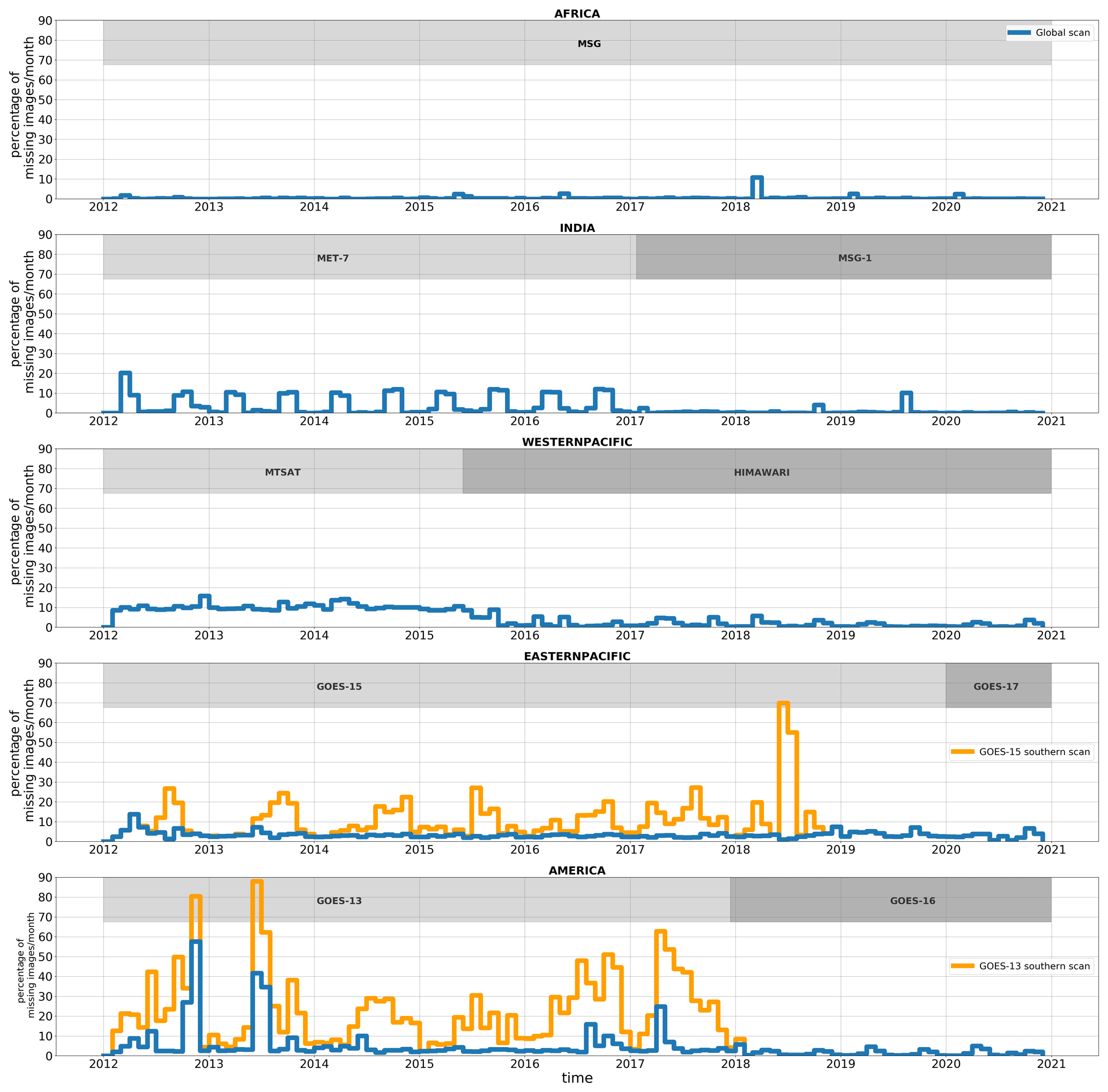
Figure 3Time series of the percentage of missing IR data per month for each region of interest and geostationary platform over the 2012–2020 period. Orange lines correspond to the availability of the southern scans of GOES-13 and GOES-15, which can be impacting by rapid-scan operation modes.
2.2 IBTrACS dataset
To understand the general characteristics and behaviors of tropical DCSs, it is important to filter out the cloud systems affected by atmospheric conditions associated with tropical cyclones. To this end, we use the IBTrACS dataset to flag DCSs that belong to a cyclonic circulation or that are classified themselves as tropical cyclones, allowing us to either filter them out of the analysis or keep them as needed.
The International Best Track Archive for Climate Stewardship (IBTrACS) version 4 is a dataset combining all of the tropical-cyclone best-track data from all the World Meteorological Organization (WMO) Regional Specialized Meteorological Centers (RSMCs), as well as other national agencies (e.g., the Joint Typhoon Warning Center) over the globe (Knapp et al., 2011). The dataset contains the tropical-cyclone location, maximum sustained wind (MSW), and minimum central pressure (MSP), as well as additional information depending on the forecast center every 6 h over the lifetime of the tropical cyclone. The tropical storm positions are interpolated in time to 3-hourly positions. In this study, we will determine whether a deep convective system is close to a tropical-cyclone meteorological event at 00:00, 06:00, 12:00, and 18:00 UTC. The combined procedure between convection systems and tropical storms is described in Sect. 3.3. The WMO standard for MSW is a 10 min average (WMO, 1983), which is used at many of the forecast centers. However, some forecast agencies use a different temporal average for MSW. A 1 min average for MSW is used at the United States forecast centers (JTWC, NHC, and CPHC), a 2 min average is used at the Chinese Meteorological Administration's Shanghai Typhoon Institute, and a 3 min average is used at the India Meteorological Department. A conversion of all MSWs to a common temporal average is then required to analyze statistically the tropical cyclones over the tropics, and several conversion factors have already been determined by Harper et al. (2008). For our study, we will use the same factor (0.88) as the one used in Kruk et al. (2010) to convert all the basins' MSWs to a 1 min average. The MSW is then used to classify all the tropical cyclones according to the Saffir–Simpson hurricane wind scale (SSHS). Over the 2012–2020 period, 825 meteorological events are classified as tropical storms. Among them, 410 tropical cyclones have been identified. A total of 208 of them reached the SSHS category 3 (90 kt) during their lifetime, 142 reached the SSHS category 4, and 17 reached the SSHS category 5 (136 kt).
3.1 The principle
The functioning of the TOOCAN (Tracking Of Organized Convection Algorithm through a 3D segmentatioN) algorithm has been fully described and explained in Fiolleau and Roca (2013a). The algorithm relies on a conceptual model of a convective system consisting of an initiation phase in which deep convective cells develop and are organized into a convective core; a maturity phase in which an anvil cloud develops in association with its convective core; and then a dissipation stage in which no more convection occurs, and the system breaks up into multiple cirriform clouds. In both the spatial and temporal domains, the optical depth of cloud cover decreases from the convective core to the edge of the anvil cloud as the brightness temperature increases. This conceptual model of a convective system corresponds to a 3D (longitude, latitude, time) cloud cluster made up of a convective core associated with its stratiform anvil and cirriform clouds evolving in the space–time domain.
To identify such a 3D cloud cluster, the algorithm works within a time sequence of IR images and applies a 3D region-growing technique to decompose the high cold-cloud shield – defined by a 235 K threshold in the spatio-temporal domain – into component DCSs. This technique consists of an iterative process of detection and dilation of convective seeds in the spatio-temporal domain to detect and track DCSs in a single 3D segmentation step. Individual convective seeds are first detected by applying a cold brightness temperature threshold set at 190 K to the volume of IR images. If any, convective seeds with a minimum lifetime duration of three frames (1 h 30 min) and exceeding 625 km2 per frame are kept and are spread in the spatio-temporal domain until reaching the intermediate cold-cloud-shield boundaries identified at a 2 K warmer BT threshold. This dilation step involves adding pixels belonging to the intermediate cold-cloud shield to all previously detected convective seeds using a 10-connected spatio-temporal neighborhood kernel operator, composed of an 8-connected spatial neighborhood and a 2-connected temporal neighborhood, to favor spatial spread over temporal spread. The pixel aggregation process is constrained by a brightness temperature difference between the edge pixels and the already identified pixel, which has to be greater than −1 K to minimize the effects of local minima. Then, a new detection is applied at the 192 K threshold to detect the convective seeds that are too warm to be identified at the previous BT threshold (190 K). If any, all the convective seeds are then spread until reaching the intermediate cold-cloud-shield boundaries at a 2 K warmer BT threshold (194 K). This iterative process of detection and dilatation is repeated with a 2 K detection step from 190 to 235 K and is stopped when all the pixels below 235 K are associated with a DCS. The very cold 190 K threshold is required to identify very deep convective cores which occur in the tropics. The multi-BT thresholds between 190 and 235 K allow us to identify the wide variety of convective cores which occur and may be more or less deep. Thanks to its spatio-temporal region-growing technique, the TOOCAN algorithm can track DCSs by suppressing split and merge artifacts, which are inherent to classic overlap-based tracking techniques, throughout their life cycles.
The first spatio-temporal volume of IR images is built by accumulating 15 d of geostationary infrared data in which TOOCAN operates. TOOCAN is applied to the next 15 d of volume images with a sliced-window technique, allowing a continuity of the tracked DCS between the two successive spatio-temporal volumes. With regards to big-data processing, the algorithm can face missing IR data. When low-quality or missing images are encountered in the time series, the data available at previous and subsequent time steps are replicated so that the tracking is carried out nominally, enabling continuity of the deep convective cloud life cycle. However, beyond a given number of successive missing images, the TOOCAN process has to be stopped, and a fresh start has to be operated at the end of the interruption. DCSs impacted by this interruption are all terminated, and new systems are considered to be initiated at the end of the interruption, causing artificial life cycles and some biases in lifetime duration distributions. Section 3.2b will detail the sensitivity of the DCS characteristics to the data availability.
Figure 4a and b show a time series of the TOOCAN segmented images from the HIMAWARI-8 IR data between 12 October 2015 at 00:00 UTC and 13 October 2015 18:00 UTC over the western Pacific Ocean. The high cold-cloud shield defined by a 235 K threshold in the infrared imagery is decomposed into several deep convective systems whose anvil clouds touch each other. The full spectrum of deep-convective-system organization is identified, ranging from small, short-lived, and isolated systems to long-lasting systems, reaching several thousands of kilometers per square meter and propagating over several hundred kilometers. For instance, the deep convective systems A and C identified over the Pacific Ocean in the time series last 60 and 137 h, respectively; reach a cold-cloud surface larger than 4.5×10⁵ km2; and propagate at a distance greater than 2000 km. The convective system B has a lifetime duration of 22.5 h, with a 2.5×10⁵ km2 maximum extent, and propagates westward over 890 km. All these very large and long-lived convective systems belong and contribute to complex convective situations, sharing common high cloud cover with various convective systems that exhibit a wide range of morphological characteristics with which they interact. Other convective systems are more isolated during their life cycles. This is the case for the DCSs D and E over the Philippines islands, which last ∼4 h and reach a maximum cold-cloud surface of ∼5500 km2. These systems are also characterized by their relative stationarity and exhibit a propagating distance of 123 and 74 km for DCSs D and E, respectively.
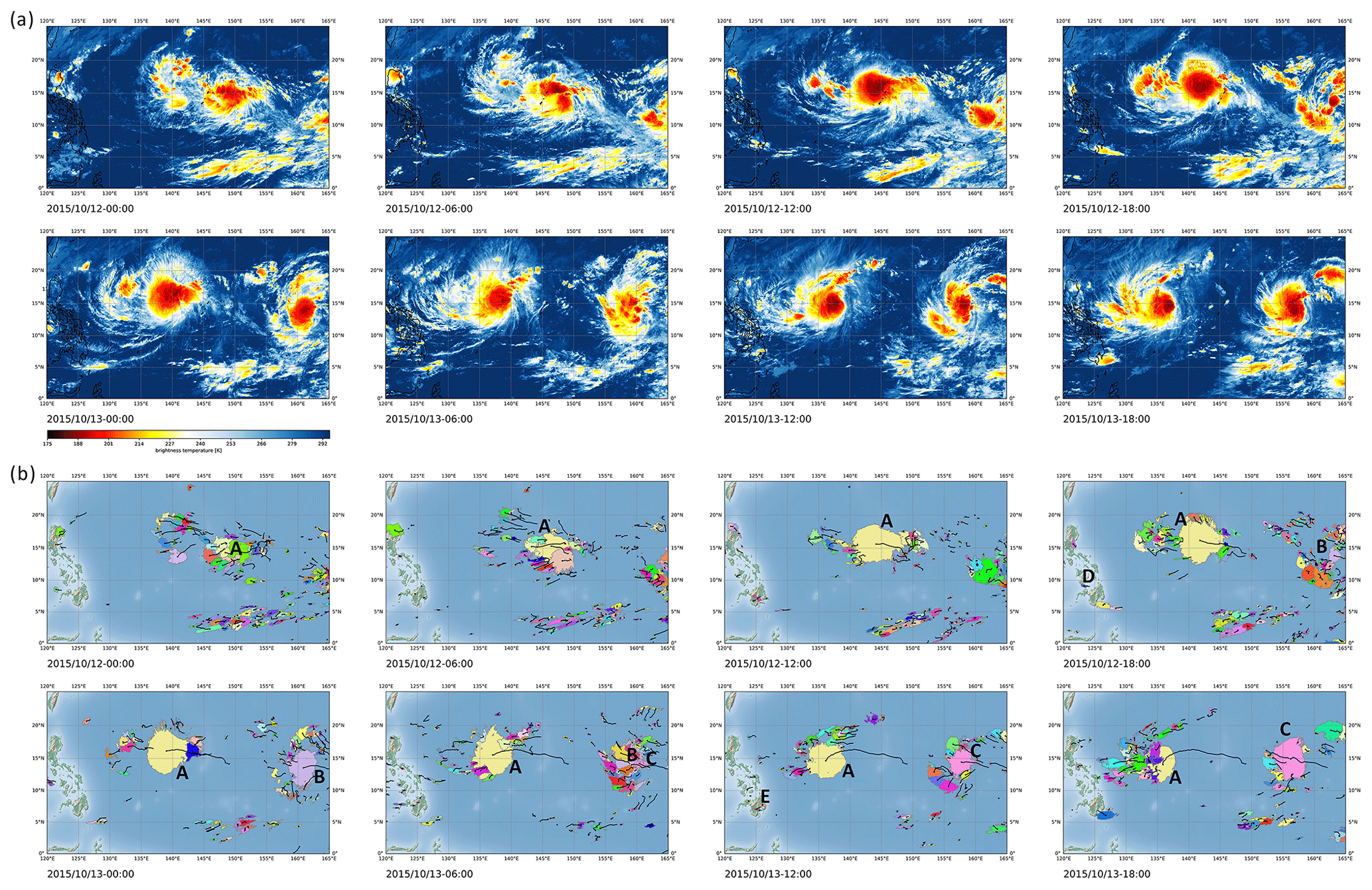
Figure 4Illustration of the TOOCAN segmentations for a convective situation which occurred in October 2015 over the western Pacific region, which is also presented in Video S1 in the Supplement (Fiolleau, 2024). (a) Infrared observation of HIMAWARI-8 every 6 h from 12 October 2015 at 00:00 UTC to 13 October 2015 at 18:00 UTC. (b) DCS segmented by the TOOCAN algorithm. Each color corresponds to a unique deep convective system. The black lines indicate the trajectories of their centers of mass since initiation.
3.2 Uncertainty estimation
In this section, we will focus on assessing the impact of radiometric errors and missing images on the performance of the segmentation and tracking of deep convective systems from IR imagery, as well as on the error propagation in statistical analyses of DCSs.
3.2.1 Uncertainty estimation due to radiometric errors
As discussed in Sect. 2.1, IR observations have been homogenized with an error lower than 1.5 K throughout the GEOring considering the intercalibration, spectral normalization, and limb-darkening corrections. In the following, we assess the impact of such a residual error on the morphological characteristics and occurrences of the DCSs. For that, the analysis is based on the MSG IR dataset over the June to September 2012 period over the 30° S–30° N, 40° W–40° E region.
From this reference dataset, we have produced an ensemble of 134 MSG-1 IR datasets over the same region and period, whose brightness temperatures have been biased by a value estimated from a Gaussian distribution with a 1.5 K standard deviation (Fig. 5). The TOOCAN algorithm has been applied to these 134 biased MSG IR datasets in order to produce an ensemble of different DCS segmentations. The average distribution of the DCS lifetime durations computed from the ensemble of MSG IR datasets (blue line) shown in Fig. 6 indicates that the maximum of the population occurs for systems lasting in the range of 0–5 h, with around 3×10⁴ DCSs. Then, the DCS population decreases as the lifetime duration increases. On average, around 320 DCSs last more than 20 h in the 134 runs of TOOCAN.
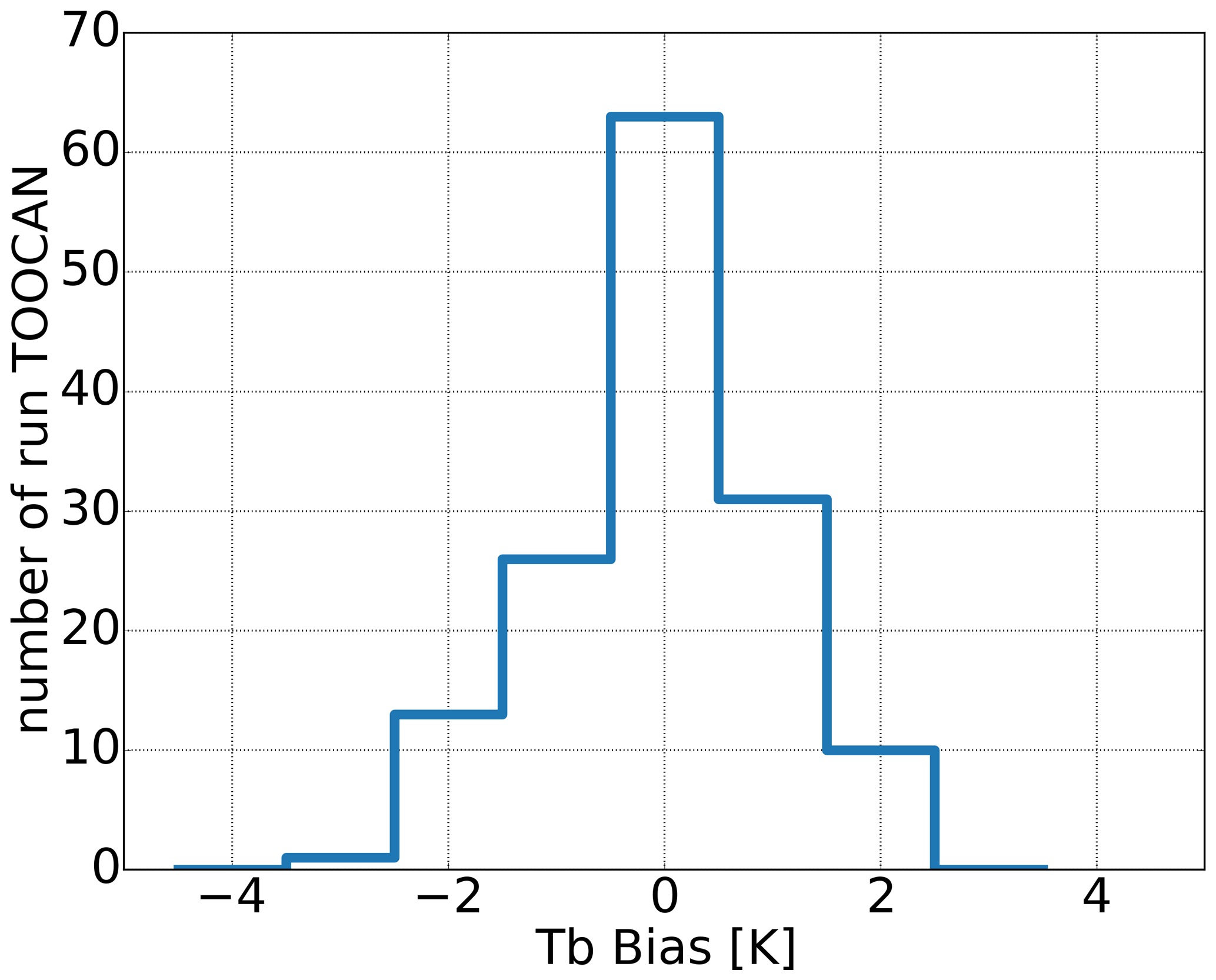
Figure 5Distribution of the brightness temperature bias applied to the MSG dataset between June to September 2012 and which has been built from a Gaussian distribution with a 1.5 K standard deviation.
The relative confidence interval (orange line) is shown Fig. 7 as a function of the lifetime duration and is computed as the absolute 95 % confidence interval divided by the DCS averaged occurrence multiplied by 100 %.
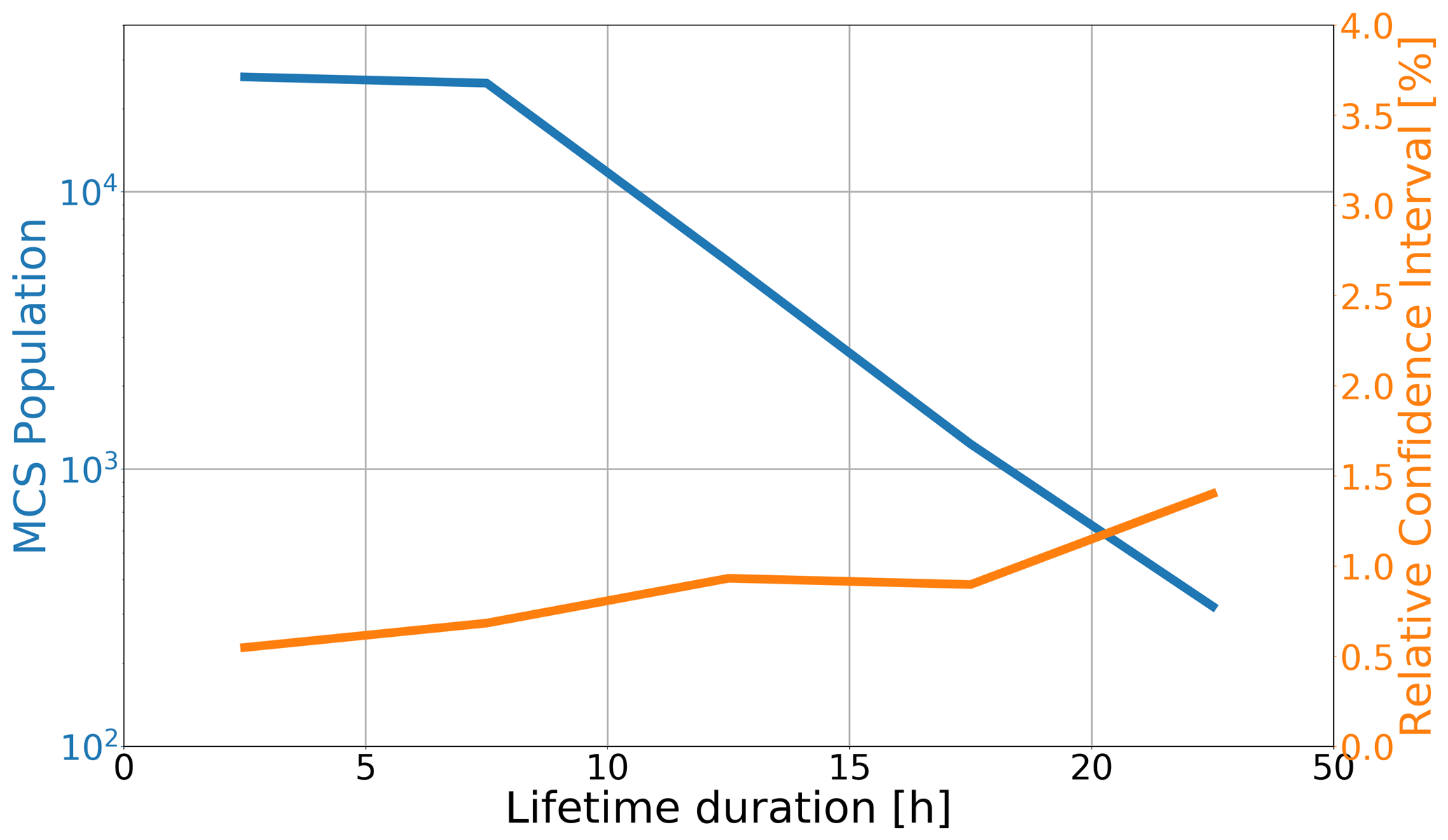
Figure 6Distribution of the average DCS lifetime duration (blue curve) computed from the 134 perturbed runs of TOOCAN applied to IR imagery of MSG from June to September in 2012 over the 30° S–30° N, 40° W–40° E region and the associated relative confidence interval (orange).
This sensitivity study reveals a small relative confidence interval whatever the bins of lifetime duration. For systems lasting less than 5 h, a 0.54 % relative confidence interval is observed for a population of ∼26 000 DCSs, meaning that we are 95 % confident that the true DCS population <5 h is between 25 859 and 26 240, with a 1.5 K residual error. This relative confidence interval increases slightly as the lifetime duration increases and as the DCS population decreases. However, the relative confidence interval remains relatively weak, with a value of ∼1.40 % for DCSs lasting more than 20 h. For these long-lasting systems, the absolute confidence interval of the DCS population is between 315 and 320.
Given the assumed 1.5 K residual bias throughout the GEOring, this analysis has shown that the IR segmentation and the DCS tracking by the TOOCAN algorithm, as well as the resulting DCS lifetime duration distributions, are not sensitive to such an error source.
3.2.2 Uncertainty estimation due to the IR geostationary data availability
The sensitivity of the DCS morphological parameters is now evaluated according to the availability of the IR geostationary images. From the point of view of cloud tracking, the major problem lies less in isolated missing data than in the number of successive missing images over time, which has an impact on the continuity and quality of cloud tracking. As seen previously in Sect. 3.1, if any missing images are found in the time series, they are replaced by the data available in the previous and following time steps, allowing convective systems to be tracked. It is then important to assess the impact of consecutive missing images on the statistics of the DCS occurrence and on the characterization of their morphological parameters.
Several scenarios arise for the DCSs facing such a time period of consecutive missing images. DCSs that were supposed to be initiated during this period of missing data are either detected at the time of resumption – in which case, their duration is artificially shortened – or cannot be identified at all. DCSs that were supposed to dissipate during this period of missing images could dissipate at the time of resumption, in which case their lifetime duration is artificially extended. There is the case of DCSs that started before the series of missing images and that are expected to persist thereafter; these can still be tracked despite this interruption. Some DCSs cannot survive the period of missing data and dissipate artificially. Smaller systems may not survive this interruption, reducing their lifetime, or their lifetime may be artificially extended due to data replication.
Also, this sensitivity study will help us to determine the threshold regarding the number of successive missing images beyond which the DCS parameters are too degraded such that the TOOCAN process has to be interrupted.
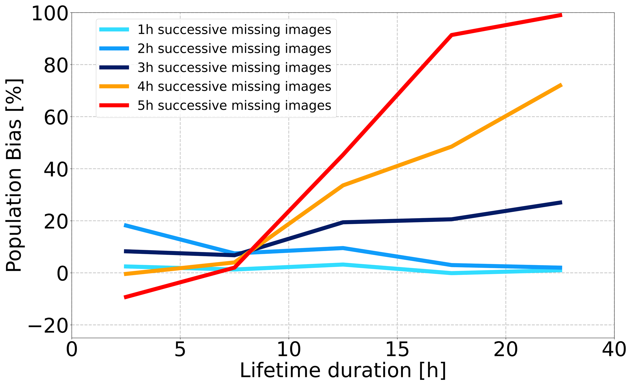
Figure 7Bias in the DCS population according to the lifetime duration between a reference run of TOOCAN applied to a complete MSG IR dataset in June–September 2012 over the 30° S–30° N, 40° W–40° E region and five runs of TOOCAN applied to a similar MSG IR dataset but degraded every day with 1, 2, 3, 4, and 5 h of successive missing images.
The same MSG IR observations over the African and Atlantic regions from June to September 2012 constitute our baseline for this analysis. This database is characterized by no missing data over the study period (Fig. 3). To better understand the impact of the missing data periods on the DCS parameters, the TOOCAN algorithm is first applied to this reference MSG IR database and then is applied to this same database but is degraded by deleting 1 h of consecutive images (between 19:00 and 20:00 UTC), 2 h of consecutive images (between 19:00 and 21:00 UTC), 3 h of consecutive images (between 19:00 and 22:00 UTC), 4 h (between 19:00 and 23:00 UTC), and finally 5 h of consecutive images (between 19:00 and 00:00 UTC) everyday. The missing-data periods are filled by duplicating the available MSG IR data just before and after the missing-data gap.
We have focused our analysis on the late hours of each day to mimic the Meteosat First Generation (MFG) eclipse seasons, during which consecutive periods of missing data occur in the evening. A gap of successive missing data in the afternoon would be more impactful for the DCS population than at night due to the diurnal cycle of initiation. However, our aim here is to determine the duration of consecutive missing data beyond which tracking the longest-lived and largest DCSs becomes ineffective, leading to degraded statistics for these systems.
Figure 7 shows the bias of DCS occurrences according to their lifetime duration between the five degraded runs of TOOCAN and the TOOCAN reference run. Up to 2 h of consecutive missing images, results indicate a bias which tends toward 0 % for the longest ones. For a run performed with 3 h of consecutive missing images, we observe an overestimation of the DCS occurrences of around 20 % for systems longer than 10 h. The biases in DCS occurrences increase drastically with the 4 and 5 h periods of consecutive missing images, and we observe an overestimation of DCS occurrences greater than 80 % and 100 %, respectively, for long DCS lifetime durations. A maximum of 3 h of consecutive missing images therefore seems to be a good compromise for ensuring tracking continuity and minimizing the impact on the DCS morphological parameters of the longest-lived systems. Note that, here, by perturbing the dataset everyday, we are exploring the worst-case scenario, which is similar to the MFG eclipse seasons.
3.3 TOOCAN implementation
The TOOCAN algorithm was applied to the harmonized infrared observations of each geostationary platform at a 30 min temporal resolution from January 2012 to December 2020. The spatial coverage of each monitored region described in Table 2 is wide enough in longitude to offer an overlapping area in relation to its neighbor's regions and is extended from 40° S to 40° N in latitude to avoid an impact of the image boundaries on the tracking of DCSs over the tropical belt. Applying a minimum buffer strip of 5° for the minimum and maximum geographical coordinates of these extended regions ensures that the shapes and trajectories of the convective systems identified in the tropical belt are not impacted by the image boundaries.
The time series of the number of days per month impacted by 1, 2, and 3 h and more than 3 h of successive missing images over the 2012–2020 period is presented in Fig. 8 for each geostationary platform and region of interest. During this period, 1.5 % of days are impacted by periods of consecutive missing data lasting more than 3 h over the entirety of the tropics and for all the geostationary platforms. From 2012 to 2017, METEOSAT-7 is the most strongly impacted by consecutive missing data, especially from early August to mid-September and from February to March, which is explained by solar eclipses. During these periods, more than 5.8 % of the days are impacted by a maximum of 3 h of consecutive missing images, and 0.73 % are impacted by a sequence of more than 3 h of consecutive missing images. From the analysis carried out in Sect. 3.2.2, we define a maximum of 3 h of consecutive missing images, above which the tracking of DCSs will be stopped. This duration of missing images is a good trade-off to track convective systems with a reasonable statistical bias in their occurrences, as seen previously, but also with a limited number of days that are impacted by such successive missing data events.
Finally, in order to have a homogeneous analysis of DCSs thereafter, the tracking process is not carried out for the southern scan of the MTSAT-1 and MTSAT-2 platforms from January 2012 to May 2015 as the 30 min time frequency requirement is not fulfilled. For a similar reason, TOOCAN is not applied to a little region between 118 and 108° W in the Southern Hemisphere, which is monitored by GOES-15 only every 3 h.
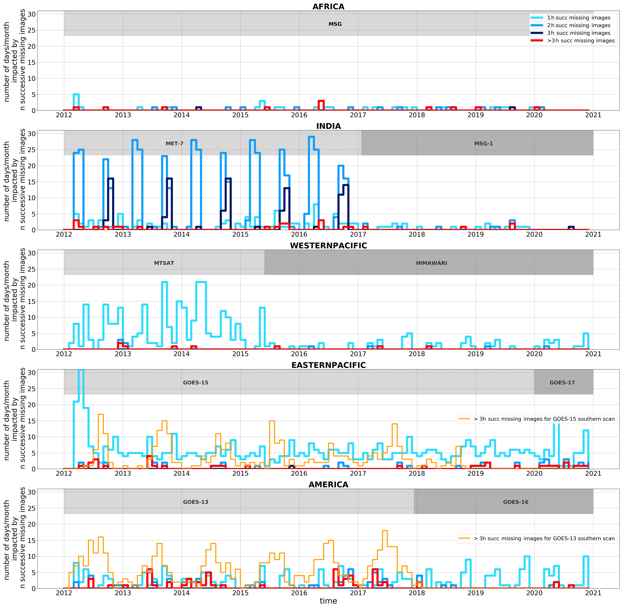
Figure 8Time series of the number of days per month impacted by 1, 2, and 3 h and more than 3 h of successive missing images between 2012 and 2020 and for the five regions of interest. The gray shading indicates the operability period for each geostationary platform.
4.1 TOOCAN dataset
The processing has given rise to a 9-year DCS database documenting convective systems identified over the tropical belt. From one side, the dataset documents the integrated morphological parameters of each identified DCS (Table B1 in the Appendix). On the other side, the morphological properties of each convective system are described every 30 min over their life cycles (Table B2). Quality controlling can raise a number of issues with the data, such as missing lines or images, which can affect the tracking of systems in various ways. The user is informed of the issues thanks to a flag coded as a five-digit number. The first digit indicates whether a DCS is born naturally or due to consecutive missing images, while the second digit indicates whether a DCS dissipates naturally or as a result of consecutive missing images. The third digit reveals whether a DCS is impacted by the edges of the image, some missing lines, or pixels. Values greater than 1 for these three digits indicate problems in initiation, dissipation, missing lines, or a problem for the detection of systems at the edges of the image. The last two digits of the quality flag represent the number of missing images during the life cycle of a given DCS. A typical conservative filtering approach would include only systems unaffected by quality-controlling issues, identified by a flag value less than 11 110.
Each cloud system has received a unique label, and the documentation of the convective systems has also been enhanced with some classifications. First, convective systems have been classified following the three categories of systems introduced in Fiolleau and Roca (2013a) and Roca et al. (2017). The deep convective systems are also categorized according to their organization – specifically, their shapes at small and large scales. In an identical way to the categories introduced by Maddox (1980) and Jirak et al. (2003), DCSs are then classified into four types: mesoscale convective complexes (MCCs), persistent elongated convective systems (PECSs), meso-β-circular convective systems (MβCCSs), and meso-β-elongated convective systems (MβECS) (Table 3). Finally, a last classification is performed by associating the DCSs with the synoptic tropical storms recorded in the IBTrACS database. As introduced in Hennon et al. (2011), a system located within a 1000 km radius of a cyclone is flagged according to the storm type and the SSHS category (Table 3).
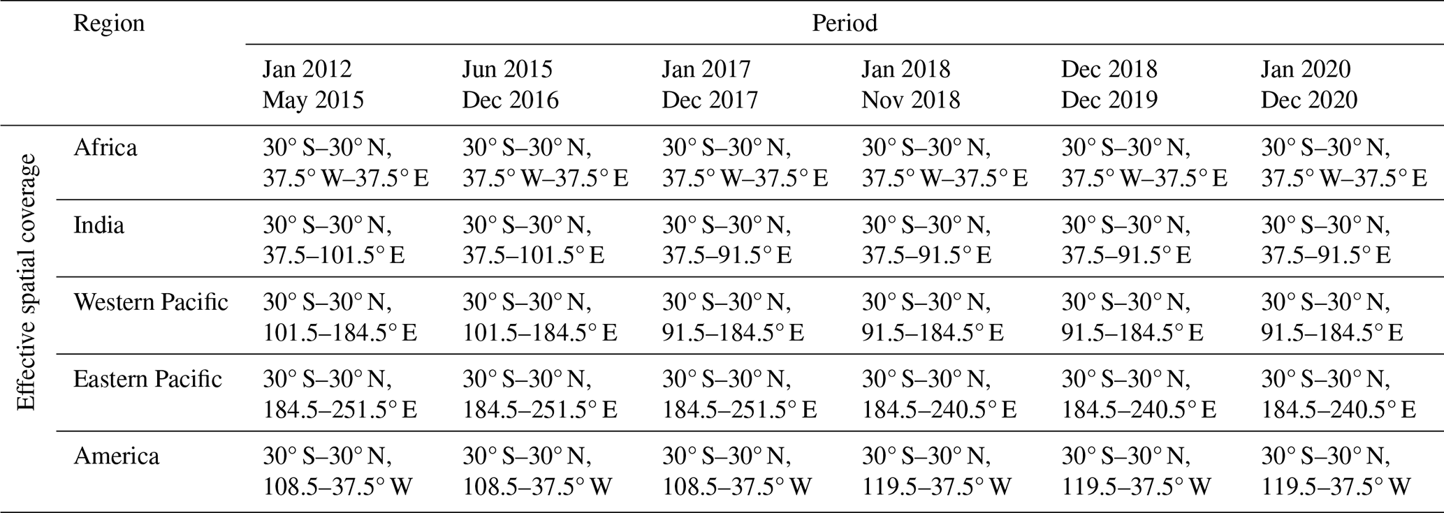
The analyses of the DCS database can be conducted on a region-per-region basis. However, to focus on the whole tropical belt, we restrict the spatial coverage for each region to prevent double=counting the same DCS identified in two adjacent geostationary platforms. Table 4 defines the spatial coverages applied to each region of interest according to the configuration of the GEOring, which evolves along the period. A quality-controlling indicator is associated with each identified DCS to indicate whether the cloud system has been impacted by interruptions or restarts, image edges, or missing images. Hence, 0.35 % of the total DCS population is found to be impacted by recovery and interruption of the tracking algorithm, with a maximum for the American (1.76 %) and eastern Pacific regions (1.47 %), explained by the rapid-scan operation modes of GOES-13 and GOES-15.
By filtering DCSs which do not pass this quality control, a total of around 15×106 DCSs were identified and tracked by TOOCAN from 2012 to 2020 over the entire tropical belt (30° S–30° N), DCSs were identified over the oceans, DCSs were identified over the continents, and 1.7×10⁶ DCSs were identified over coastal regions. Oceanic convective systems are described by a slightly longer average lifetime duration (6.25 h) than continental systems (6 h). Oceanic systems can last up to 102 h, while the continental ones reach a maximum of 43.5 h. A large majority of convective systems are characterized by a maximum area between 1×10³ and 2×10⁵ km2, but some of them can reach a maximum extent up to 2.3×10⁶ km2 over the ocean and 1.3×10⁶ km2 over continents.
Table 3DCS classifications and physical characteristics used in the TOOCAN database.
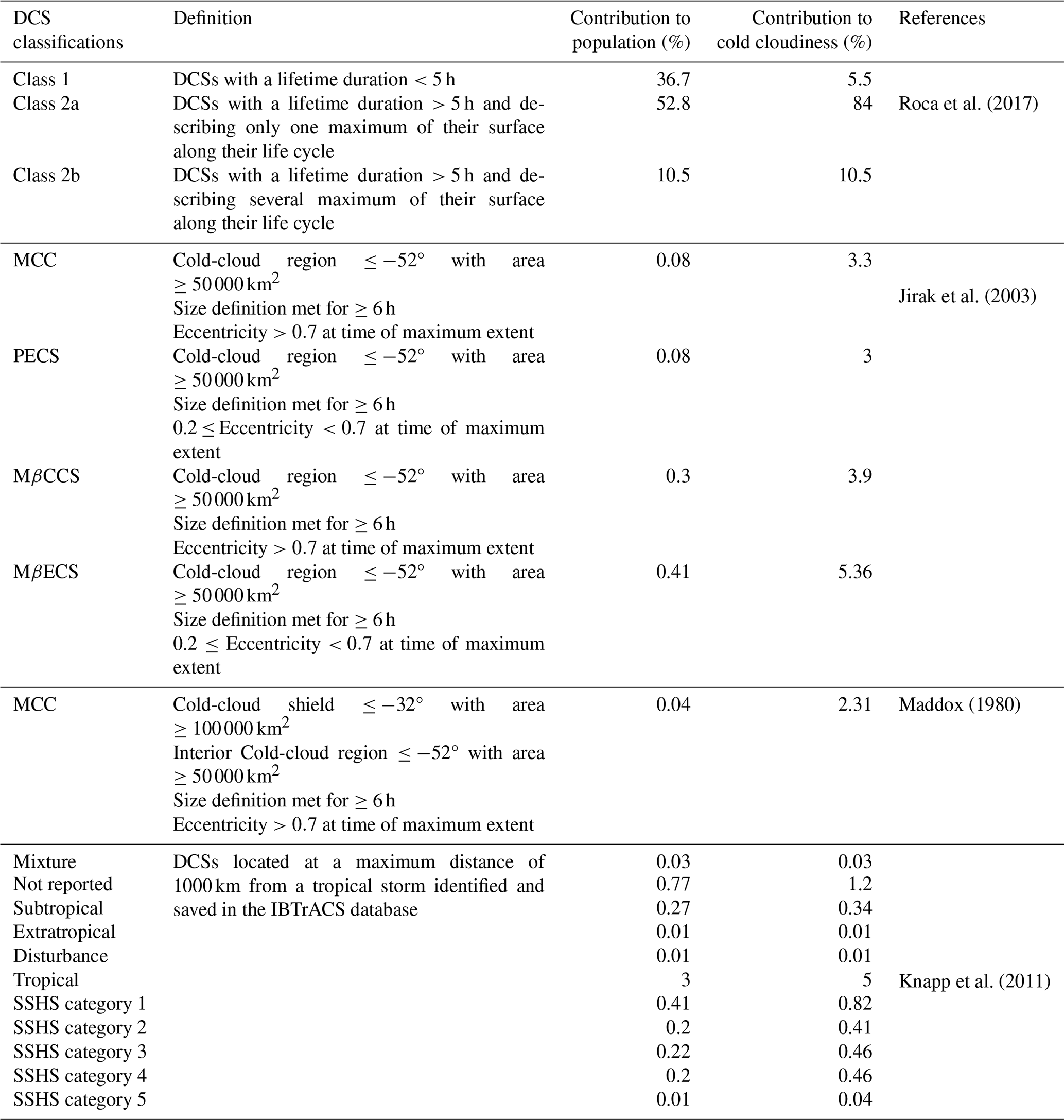
Regarding the system classifications, systems belonging to class 1 contribute to 36.7 % of the total population but only 5.5 % of the cold-cloudiness area (Table 3). Class-2a convective systems contribute to 52.8 % of the total population and 84 % of the cold-cloudiness area, which is consistent with the results obtained in Roca et al. (2017). Convective systems classified as MCC according to the definition given by Jirak et al. (2003) represent only 0.08 % of the total population but contribute to 3.3 % of the cold-cloudiness area. Finally, a total of 156 594 DCSs are included within a 1000 km radius of a tropical cyclone (1 % of the total population), and only 2081 of them are associated with a category-5 cyclone (SSHS).
Table 4Effective spatial coverage to be applied to each region and for the periods corresponding to specific GEOring configurations for a tropical-belt analysis.
4.1.1 An illustration of the TOOCAN database
The annual climatology of the occurrence and morphological characteristics of deep convective systems is shown Fig. 9 in a phase diagram using lifetime duration and maximum extent as coordinates. Here, DCSs within a 1000 km radius of a tropical cyclone have been removed from this analysis.
The distribution is described by systems lasting a few hours and reaching around 1000 km2 to systems lasting several days and reaching up to a few millions square kilometers (Fig. 9a). While a strong relationship is observed between lifetime duration and the maximum extent at the first order, it is also to be noticed that the same lifetime duration can be associated with a large spread of maximum extent. Figure 9b also shows that the larger the cloud shield is, the colder the temperatures at the top of the cloud are and, therefore, the deeper the cloud is. Similarly to Roca et al. (2024), both land and ocean distributions are described by a “V” pattern, with two branches associated with the warmer systems. The shape of the cloud shield of the system is shown in Fig. 9c, with the distribution of the eccentricity of the cloud shield at the time of maximum extent along the life cycle. The eccentricity is defined by the ratio of the semi-minor axis to the semi-major axis of the equivalent ellipse. While the largest and coldest deep convective systems are characterized by circularity of their cold-cloud shields (eccentricity >0.7), the warmer DCSs located in the two branches of the V pattern are more characterized by linear shapes in their cold-cloud shields (eccentricity <0.5). The distribution of the average speed according to maximum extent and lifetime duration is shown Fig. 9d. The fastest systems are found in the upper part of the distribution, while the slowest are found in its lower part. These features are more pronounced over the ocean compared to over land.
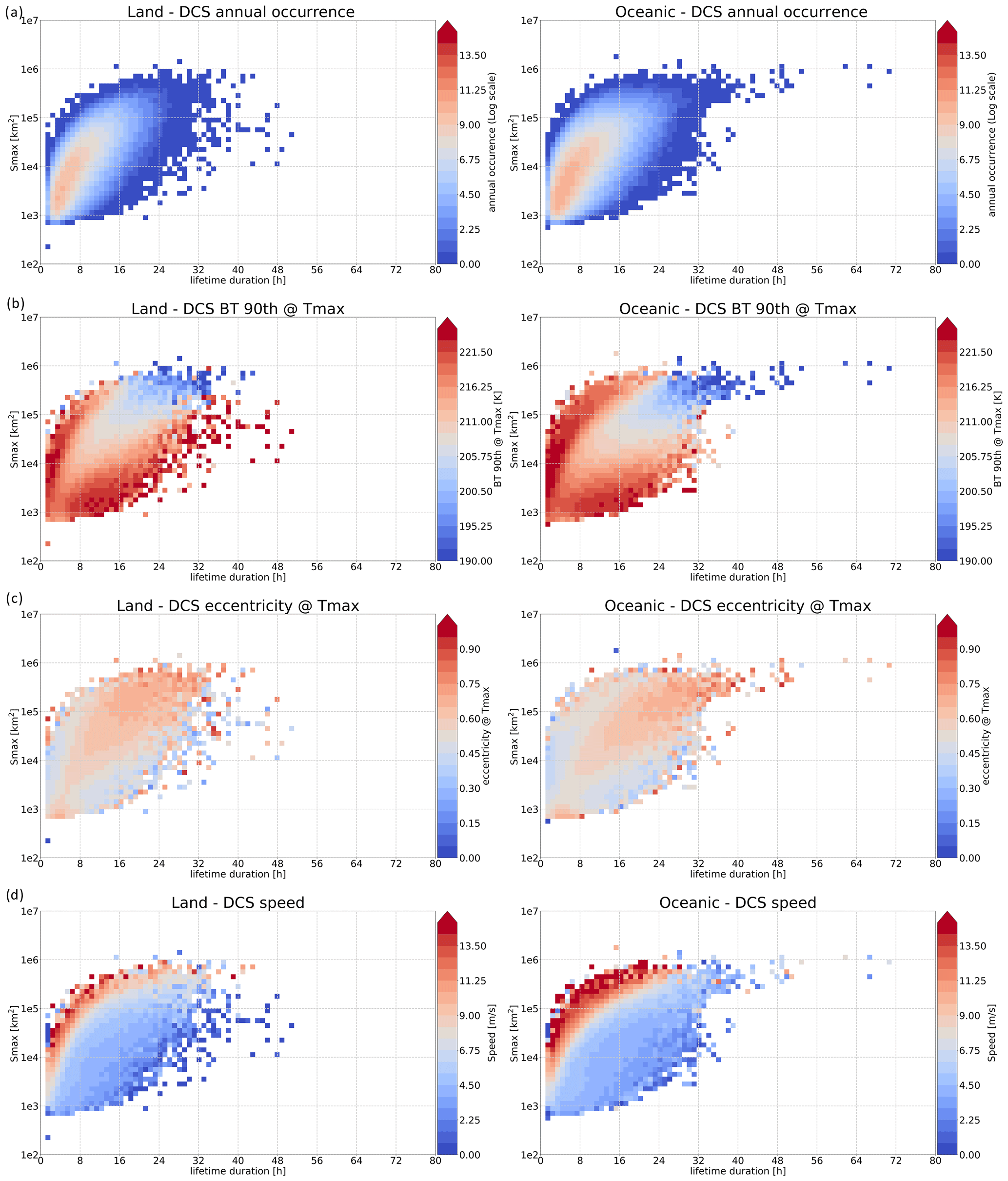
Figure 9(a) Annual occurrence of the deep convective systems for continental (left) and oceanic regions, (b) 90th percentile of the cluster brightness temperature at the time of maximum extent, (c) eccentricity of the cluster at the time of maximum extent, (d) movement speed of the deep convective system.
4.2 CACATOES dataset
The CACATOES database is a level-3 product derived from the TOOCAN database, allowing a Eulerian view of the deep-convective-system properties from a grid box perspective. The method was introduced and used in several studies (Roca and Fiolleau, 2020; Berthet et al., 2017; Roca et al., 2014) and makes it easier to conduct the joint analysis with auxiliary data gridded on the same daily 1° × 1° grid box. The integrated morphological parameters of each DCS are gridded into a 1° × 1° daily grid (Table C1). For that, the full-resolution pixels composing the convective systems identified within the TOOCAN segmented images are projected onto each daily 1° × 1° grid box. The cold-cloudiness fraction of each DCS which overpasses a given daily grid box is computed, and their morphological properties are assigned to that particular grid box. If the cold-cloud shield of a given DCS overpasses more than one daily grid box, the cold cloudiness of this given DCS is then distributed onto each of the associated daily grid boxes. Similarly, when a system lasts for more than 1 d, the associated cold cloudiness is distributed over all the relevant days. Owing to the DCS propagation, cold-cloud surfaces, and lifetime durations, several systems can overpass the same 1° × 1° grid box in 1 d. In that case, all together, they contribute to the total cold cloudiness of this given grid box. It has been defined that a maximum of 25 individual systems can overpass each grid box in a day. Within a given daily 1° × 1° grid box, the DCS morphological properties are finally sorted according to their cold-cloudiness occupation so that the most representative DCSs can be easily identified. Roca and Fiolleau (2020) have shown that a couple of DCSs significantly impact each daily 1° × 1° grid box, while most of the other systems make very small contributions to the cold cloudiness. The statistical analysis of the DCS morphological parameters requires special care when considered in a Eulerian framework. For instance, a DCS with a long lifetime duration may overpass only a few moments and a small footprint of a daily 1° × 1° grid box, skewing the statistical results. Therefore, the average of a given morphological parameter over a region and time period has to be weighted using the actual-cloud occupation of each system within each grid box. Similarly, the computation of the DCS population over a region and time period has to be considered with caution and can be computed by the sum of all the systems' cold-cloud fractions overpassing the daily grid boxes.
4.2.1 An illustration of the CACATOES database
Figure 10 shows the daily 1° × 1° spatial distribution of the DCS densities calculated from January 2012 to December 2020 over the entire tropical belt. The hatched areas indicate that the southern part of the western Pacific region and a southern band between 118 and 108° W of the eastern Pacific region were affected by missing data from January 2012 to May 2015 and from January 2012 to November 2017, respectively. The DCS densities of these two specific regions were then computed with a lower number of days being involved. This may impact the patterns of DCS density; therefore, we would like to emphasize to future users that the analysis should be carried out with caution. Also, note that the map was built considering only days not impacted by any tracking interruptions over any part of the tropical region, corresponding to 61.5 % of the total number of days over the entire 2012–2020 period. This number is mainly explained by the interruption of the southern scans of GOES-13 and GOES-15 due to rapid-scan operations.
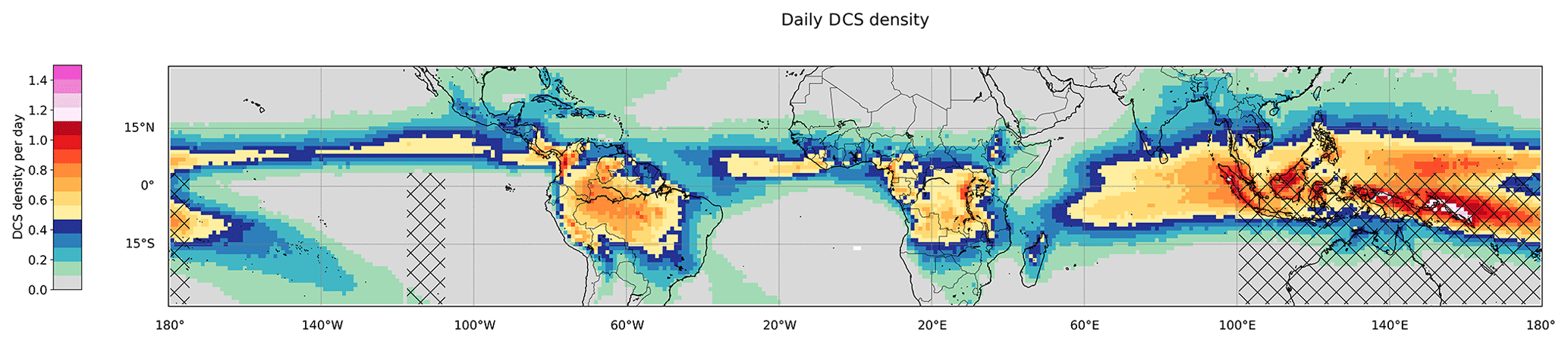
Figure 10Map of the deep-convective-system density per day for a 1° × 1° grid box from January 2012 to December 2020. The hatched areas indicate missing data over the southern parts of the western and eastern Pacific regions from January 2012 to May 2015 and from January 2012 to November 2017, respectively.
The geographical distribution of DCS density per day is consistent with previous DCS climatologies based on other definitions, algorithms, and satellite observations from either local or global studies (Mohr and Zipser, 1996; Liu et al., 2008; Feng et al., 2021; Huang et al., 2018). A zonal and homogeneous structure occurs over the Atlantic Ocean, extending from the Guinean coast to 40° W (Machado et al., 1992). The Indian Ocean shows a large and zonally structured region, corresponding to the intertropical convergence zone (ITCZ) (Roca and Ramanathan, 2000). On the continent, the western African deep convective systems extend no further north than 17° N, and the Indian Ocean convective systems extend to the foot of the Himalayas. DCSs are also numerous over the western half of the maritime continent (Williams and Houze, 1987), with similar occurrences to those of Southeast Asia and the Philippines. The eastern Pacific ITCZ is also characterized by a large occurrence of DCSs.
5.1 TOOCAN Data format
The TOOCAN database is composed of two types of files. Regional TOOCAN segmented images at a 0.04° spatial resolution are produced every 30 min in a NetCDF4 format, with metadata following the Climate and Forecast (CF) convention version 1.6 and the Attribute Convention for Dataset Discovery (ACDD) version 1.3. The TOOCAN segmented image files contain the following information:
-
DCS_number. These are labeled pixels of the convective systems identified by the TOOCAN algorithm.
-
Latitude. This constitutes the latitude values of the grid in degrees, ranging between −40 and 40° N).
-
Longitude. This constitutes the longitude values of the grid in degrees.
-
Time. This is the starting-time scan of the image (in seconds) from 1 January 1970.
-
Scan time. This is the time (in seconds) since 1 January 1970 at which each line of the TOOCAN segmented image is scanned by the geostationary platform.
Regional and monthly tracking files are produced in a NetCDF4 format, with metadata following the Climate and Forecast (CF) convention version 1.6 and the Attribute Convention for Dataset Discovery (ACDD) version 1.3 to document the DCS integrated morphological parameters, as well as the DCS parameters at each 30 min time step of their life cycles. Note that similar regional and monthly tracking files have also been produced in an ASCII format in order to ensure continuity with previous versions of the TOOCAN database.
Only the deep convective systems which are initiated in a given month are stored in the corresponding monthly tracking file. If a DCS is initiated in a given month but its dissipation extends beyond the end of that same month, the complete life cycle of this DCS is recorded in the file for the month corresponding to its birth. Each DCS is described by a unique label, and the link can be easily established between a given DCS described in a monthly tracking file and the pixels constituting this given DCS within the TOOCAN segmented images.
5.2 CACATOES data format
The daily 1° × 1° CACATOES tropical monthly files, describing the characteristics of DCSs overpassing the daily 1° × 1° longitude–latitude grid boxes, are also produced in a NetCDF4 format with metadata following the Climate and Forecast (CF) convention version 1.6 and the Attribute Convention for Dataset Discovery (ACDD) version 1.3.
The TOOCAN database is available over the 2012–2020 period for each region of interest with a 40° S–40° N latitudinal coverage (eastern Pacific, America, Africa, India, western Pacific) at the following link: https://doi.org/10.14768/1be7fd53-8b81-416e-90d5-002b36b30cf8 (Fiolleau and Roca, 2023a). The CACATOES database, derived from the TOOCAN dataset, is available for the 2012–2020 period over the whole tropical belt (30° S–30° N) at the following link: https://doi.org/10.14768/98569eea-d056-412d-9f52-73ea07b9cdca (Fiolleau and Roca, 2023b). The 2012–2020 homogenized infrared geostationary level-1C dataset described in this paper, to which the TOOCAN algorithm has been applied, can be accessed via the repository under the following data DOI: https://doi.org/10.14768/93f138f5-a553-4691-96ed-952fd32d2fc3 (Fiolleau and Roca, 2023c). The DOI landing pages provide the up-to-date information on how to access the database, as well as a number of useful references for users.
A unique database of the deep convective systems and their morphological characteristics covering the 2012–2020 period over the intertropical belt has been introduced. The DCS morphology is obtained thanks to the TOOCAN tracking algorithm applied to a homogenized GEOring infrared archive. The homogenized GEOring database has been built from level-1 data of a fleet of geostationary platforms originating from various sources. The temporal and spatial resolutions of this GEOring archive are, respectively, 30 min and 0.04°. The GEOring dataset has been further intercalibrated; spectrally adjusted; and limb-darkening corrected, specifically for the high cold-cloud shield, based on a common reference, the IR channel of the ScaRaB radiometer on board the Megha-Tropiques following the methodology introduced in Fiolleau et al. (2020). The global homogeneity of the IR GEOring dataset is then characterized by a residual error of 1.33 K. Over the 9-year period, the configuration of the geostationary fleet drastically changed. In June 2015, MTSAT was replaced by HIMAWARI-8 over the western Pacific Ocean. In January 2017, the end of the operation of METEOSAT-7 corresponded to the arrival of MSG-1. Finally, GOES-16 and GOES-17 have became operational, respectively, in December 2017 over the Americas and in January 2020 for the eastern Pacific Ocean.
An assessment of the sensitivity of the DCSs identified by TOOCAN to the radiometric errors of the homogenized GEOring has been carried out. This analysis has shown a very small impact of a 1.5 K residual error on the DCS occurrences, whatever their lifetime durations. Similarly, we have evaluated the impact of consecutive missing images on the quality of the DCS tracking. By filling the missing data periods with the available IR data just before and after the missing-data gap, we have shown that, for a period of up to 3 h of consecutive missing images, the impact on the DCS occurrences is relatively small. Hence, the occurrence of systems lasting more than 10 h is skewed by 20 % for a 3 h period of consecutive missing images. Beyond 3 h of consecutive missing images, the impact on the DCS segmentation is too high, and the tracking process has to be stopped.
The TOOCAN algorithm has then been processed on the homogenized GEOring IR data over the 2012–2020 period and for the latitude band of 40° S–40° N. The resulting database gives access to the integrated morphological parameters of each DCS (location and time of initiation and dissipation, lifetime duration, propagated distance, cold-cloud maximum extent, etc.), as well as the evolution of the morphological properties along the DCS life cycles. The DCSs located near a cyclone identified in the IBTrACS database (Knapp et al., 2010) have been flagged. A total of 15×106 DCSs have been detected and tracked by TOOCAN over the tropical regions and the 9-year period. The analysis of the DCS database over the tropical oceans and continents shows the large variety of DCS characteristics and organizations encountered. DCSs can last for a few hours up to several days and are distributed by cloud surfaces from 1000 km2 to a few million square kilometers. Oceanic DCSs are described by a longer lifetime duration and larger cold-cloud surfaces. Over both regions, while a strong relationship is observed between lifetime duration and maximum surface extent in the first order, we can also notice a large spectrum of maximum extent for a given lifetime duration. The 2D spatial distribution of DCS density over the tropics is also in line with previous DCS climatologies produced from other formulation of tracking algorithms and geostationary IR datasets (Feng et al., 2021; Huang et al., 2018; Rajagopal et al., 2023).
Below, we show an example of a header of the NetCDF4 file for the TOOCAN monthly tracking file.
dimensions:
DCS = 40 915;
time = UNLIMITED; // (1523 currently)
variables:
int time(time);
time:units = “seconds since 1970-01-01”;
time:long_name = “time”;
int DCS(DCS);
DCS:units = “none”;
DCS:long_name = “Label of the Deep Convective Systems”;
int INT_DCSnumber(DCS);
INT_DCSnumber:_FillValue = −999;
INT_DCSnumber:units = “”;
INT_DCSnumber:long_name = “Label of the DCS in the TOOCAN segmented images”;
int INT_DCS_qualitycontrol(DCS);
INT_DCS_qualitycontrol:_FillValue = −999;
INT_DCS_qualitycontrol:units = “”;
INT_DCS_qualitycontrol:long_name = “Quality control on the DCS initiation/dissipation…”;
int INT_classif(DCS);
INT_classif:_FillValue = −999;
INT_classif:units = “”;
INT_classif:long_name = “Classification of the DCS according to Roca et al. (2017)”;
INT_classif:flag_values = 1, 2, 3;
INT_classif:flag_meanings = “DCS with a duration <5 h, DCS with a duration ≥5 h and described by a single maximum of their cold surfaces along their life cycles, DCS with a duration ≥5 h and described by several maximums of their cold surfaces along their life cycles”;
float INT_duration(DCS);
INT_duration:_FillValue = −999.f;
INT_duration:units = “hr”;
INT_duration:long_name = “DCS lifetime duration”;
int INT_UTC_timeInit(DCS);
INT_UTC_timeInit:_FillValue = −999;
INT_UTC_timeInit:units = “seconds since 1st January 1970”;
INT_UTC_timeInit:long_name = “Universal Time of the DCS initiation”;
int INT_localtime_Init(DCS);
INT_localtime_Init:_FillValue = −999;
INT_localtime_Init:units = “seconds since 1st January 1970”;
INT_localtime_Init:long_name = “Local time of the DCS initiation”;
float INT_lonInit(DCS);
INT_lonInit:_FillValue = −999.f;
INT_lonInit:units = “degrees”;
INT_lonInit:long_name = “Longitude of the DCS center of mass at its initiation”;
float INT_latInit(DCS);
INT_latInit:_FillValue = −999.f;
INT_latInit:units = “degrees”;
INT_latInit:long_name = “Latitude of the DCS center of mass at its initiation”;
int INT_UTC_timeEnd(DCS);
INT_UTC_timeEnd:_FillValue = −999;
INT_UTC_timeEnd:units = “seconds since 1st January 1970”;
INT_UTC_timeEnd:long_name = “Coordinated Universal Time of the DCS dissipation”;
int INT_localtime_End(DCS);
INT_localtime_End:_FillValue = −999;
INT_localtime_End:units = “seconds since 1st January 1970”;
INT_localtime_End:long_name = “Local time of the DCS dissipation”;
float INT_lonEnd(DCS);
INT_lonEnd:_FillValue = −999.f;
INT_lonEnd:units = “degrees”;
INT_lonEnd:long_name = “Longitude of the DCS center of mass at its dissipation”;
float INT_latEnd(DCS);
INT_latEnd:_FillValue = −999.f;
INT_latEnd:units = “degrees”;
INT_latEnd:long_name = “Latitude of the DCS center of mass at its dissipation”;
float INT_velocityAvg(DCS);
INT_velocityAvg:_FillValue = −999.f;
INT_velocityAvg:units = “m/s”;
INT_velocityAvg:long_name = “Average velocity of the DCS from its initiation to its dissipation”;
float INT_distance(DCS);
INT_distance:_FillValue = −999.f;
INT_distance:units = “km”;
INT_distance:long_name = “DCS propagated distance”;
float INT_lonmin(DCS);
INT_lonmin:_FillValue = −999.f;
INT_lonmin:units = “degrees”;
INT_lonmin:long_name = “Minimum longitude of the DCS along its life cycle”;
float INT_lonmax(DCS);
INT_lonmax:_FillValue = −999.f;
INT_lonmax:units = “degrees”;
INT_lonmax:long_name = “Maximum latitude of the DCS along its life cycle”;
float INT_latmin(DCS);
INT_latmin:_FillValue = −999.f;
INT_latmin:units = “degrees”;
INT_latmin:long_name = “Minimum longitude of the DCS along its life cycle”;
float INT_latmax(DCS);
INT_latmax:_FillValue = −999.f;
INT_latmax:units = “degrees”;
INT_latmax:long_name = “Maximum latitude of the DCS along its life cycle”;
float INT_tbmin(DCS);
INT_tbmin:_FillValue = −999.f;
INT_tbmin:units = “K”;
INT_tbmin:long_name = “Minimum brightness temperature of the DCS along its life cycle”;
int INT_surfmaxPix_235K(DCS);
INT_surfmaxPix_235K:_FillValue = −999;
INT_surfmaxPix_235K:units = “number of pixels”;
INT_surfmaxPix_235K:long_name = “Maximum cold cloud surface at 235K reached by the DCS along its life cycle”;
float INT_surfmaxkm2_235K(DCS);
INT_surfmaxkm2_235K:_FillValue = −999.f;
INT_surfmaxkm2_235K:units = “km2”;
INT_surfmaxkm2_235K:long_name = “Maximum cold cloud surface at 235 K reached by the DCS along its life cycle”;
float INT_surfmaxkm2_220K(DCS);
INT_surfmaxkm2_220K:_FillValue = −999.f;
INT_surfmaxkm2_220K:units = “km2km2”;
INT_surfmaxkm2_220K:long_name = “Maximum cold cloud surface at 220 K reached by the DCS along its life cycle”;
float INT_surfmaxkm2_210K(DCS);
INT_surfmaxkm2_210K:_FillValue = −999.f;
INT_surfmaxkm2_210K:units = “km2”;
INT_surfmaxkm2_210K:long_name = “Maximum cold cloud surface at 210 K reached by the DCS along its life cycle”;
float INT_surfmaxkm2_200K(DCS);
INT_surfmaxkm2_200K:_FillValue = −999.f;
INT_surfmaxkm2_200K:units = “km2”;
INT_surfmaxkm2_200K:long_name = “Maximum cold cloud surface at 200 K reached by the DCS along its life cycle”;
float INT_surfcumkm2_235K(DCS);
INT_surfcumkm2_235K:_FillValue = −999.f;
INT_surfcumkm2_235K:units = “km2”;
INT_surfcumkm2_235K:long_name = “Cumulated cold cloud surface at 235 K along the DCS life cycle”;
int INT_classif_JIRAK(DCS);
INT_classif_JIRAK:_FillValue = -999;
INT_classif_JIRAK:units = “none”;
INT_classif_JIRAK:long_name = “DCS classification according to the JIRAK definition (Jirak et al., 2003)”;
INT_classif_JIRAK:flag_values = 0, 1, 2, 3, 4;
INT_classif_JIRAK:flag_meanings = “no classification,MCC,PECS,MBCC,MBECC”;
int INT_classif_MADDOX(DCS);
INT_classif_MADDOX:_FillValue = −999;
INT_classif_MADDOX:units = “none”;
INT_classif_MADDOX:long_name = “DCS classification according to the MADDOX definition Maddox (1980)”;
INT_classif_MADDOX:flag_values = 0, 1, 2, 3, 4, 5, 6, 7, 8, 9, 10, 11, 12, 13, 14, 15;
INT_classif_MADDOX:flag_meanings = “no matching with TS, Mixture, Not reported, disturbance, subtropical storm, extratropical storm, tropical storm, cyclone SSHS category 1, cyclone SSHS category 2, cyclone SSHS category 3, cyclone SSHS category 4, cyclone SSHS category 5”;
int INT_TS_number_IBTRACS(DCS);
INT_TS_number_IBTRACS:_FillValue = −999;
INT_TS_number_IBTRACS:units = “none”;
INT_TS_number_IBTRACS:long_name = “number of the Tropical Storm in the IBTRACS database associated with the DCS within a 1000 km radius”;
int INT_TS_nature_IBTRACS(DCS);
INT_TS_nature_IBTRACS:_FillValue = −999;
INT_TS_nature_IBTRACS:units = “none”;
INT_TS_nature_IBTRACS:long_name = “nature of the Tropical Storm in the IBTRACS database”;
float INT_TS_mindistance_IBTRACS(DCS);
INT_TS_mindistance_IBTRACS:_FillValue = −999.f;
INT_TS_mindistance_IBTRACS:units = “km2”;
INT_TS_mindistance_IBTRACS:long_name = “Distance of the DCS to the Tropical Storm (maximum distance: 1000 km)”;
int QCgeo_IRimage(time);
QCgeo_IRimage:_FillValue = −999;
QCgeo_IRimage:units = “nodimension”;
QCgeo_IRimage:long_name = “Quality control on the GEO IR data”;
QCgeo_IRimage:flag_values = 0, 1, 2;
QCgeo_IRimage:flag_meanings = “Missing GEO IR data, The Full GEO IR data OK, The Only North scan of GEO IR data OK”;
float LC_tbmin(DCS, time);
LC_tbmin:_FillValue = −999.f;
LC_tbmin:units = “K”;
LC_tbmin:long_name = “Minimum brightness temperature”;
float LC_tbavg_235K(DCS, time);
LC_tbavg_235K:_FillValue = −999.f;
LC_tbavg_235K:units = “K”;
LC_tbavg_235K:long_name = “Average brightness temperature at 235 K”;
float LC_tbavg_208K(DCS, time);
LC_tbavg_208K:_FillValue = −999.f;
LC_tbavg_208K:units = “K”;
LC_tbavg_208K:long_name = “Average brightness temperature at 208 K”;
float LC_tbavg_200K(DCS, time);
LC_tbavg_200K:_FillValue = −999.f;
LC_tbavg_200K:units = “K”;
LC_tbavg_200K:long_name = “Average brightness temperature at 200 K”;
float LC_tb90th(DCS, time);
LC_tb90th:_FillValue = −999.f;
LC_tb90th:units = “K”;
LC_tb90th:long_name = “Tb 90th percentile”;
int LC_UTC_time(DCS, time);
LC_UTC_time:_FillValue = −999;
LC_UTC_time:units = “seconds since 1st January 1970”;
LC_UTC_time:long_name = “Coordinated Universal Time of the DCS”;
int LC_localtime(DCS, time);
LC_localtime:_FillValue = −999;
LC_localtime:units = “seconds since 1st January 1970”;
LC_localtime:long_name = “Local Time of the DCS”;
float LC_lon(DCS, time);
LC_lon:_FillValue = −999.f;
LC_lon:units = “degrees”;
LC_lon:long_name = “longitude of the DCS center of mass”;
float LC_lat(DCS, time);
LC_lat:_FillValue = −999.f;
LC_lat:units = “degrees”;
LC_lat:long_name = “latitude of the DCS center of mass”;
int LC_x(DCS, time);
LC_x:_FillValue = −999;
LC_x:units = “pixels”;
LC_x:long_name = “Column of the DCS center of mass”;
int LC_y(DCS, time);
LC_y:_FillValue = −999;
LC_y:standard_name = “pixels”;
LC_y:long_name = “Line of the DCS center of mass”;
float LC_velocity(DCS, time);
LC_velocity:_FillValue = −999.f;
LC_velocity:units = “m/s”;
LC_velocity:long_name = “instantaneous velocity”;
float LC_semiminor_235K(DCS, time);
LC_semiminor_235K:_FillValue = −999.f;
LC_semiminor_235K:units = “km”;
LC_semiminor_235K:long_name = “Semi-minor axis of the equivalent ellipse at a 235 K threshold”;
float LC_semimajor_235K(DCS, time);
LC_semimajor_235K:_FillValue = −999.f;
vLC_semimajor_235K:units = “km”;
LC_semimajor_235K:long_name = “Semi-major axis of the equivalent ellipse at a 235 K threshold”;
float LC_ecc_235K(DCS, time);
LC_ecc_235K:_FillValue = −999.f;
LC_ecc_235K:units = “semiminor/semimajor”;
LC_ecc_235K:long_name = “Eccentricity of the equivalent ellipse at a 235 K threshold”;
float LC_orientation_235K(DCS, time);
LC_orientation_235K:_FillValue = −999.f;
LC_orientation_235K:units = “degrees”;
LC_orientation_235K:long_name = “orientation of the equivalent ellipse at a 235 K threshold”;
float LC_semiminor_220K(DCS, time);
LC_semiminor_220K:_FillValue = −999.f;
LC_semiminor_220K:units = “km”;
LC_semiminor_220K:long_name = “Semi-minor axis of the equivalent ellipse at a 220 K threshold”;
float LC_semimajor_220K(DCS, time);
LC_semimajor_220K:_FillValue = −999.f;
LC_semimajor_220K:units = “km”;
LC_semimajor_220K:long_name = “Semi-major axis of the equivalent ellipse at a 220 K threshold”;
float LC_ecc_220K(DCS, time);
LC_ecc_220K:_FillValue = −999.f;
LC_ecc_220K:units = “semiminor/semimajor”;
LC_ecc_220K:long_name = “Eccentricity of the equivalent ellipse at a 220 K threshold”;
float LC_orientation_220K(DCS, time);
LC_orientation_220K:_FillValue = −999.f;
LC_orientation_220K:units = “degrees”;
LC_orientation_220K:long_name = “orientation of the equivalent ellipse at a 220 K threshold”;
int LC_surfPix_235K(DCS, time);
LC_surfPix_235K:_FillValue = −999;
LC_surfPix_235K:units = “number of pixels”;
LC_surfPix_235K:long_name = “Cold cloud surface in number of pixels of the convective cluster for a 235 K threshold”;
int LC_surfPix_210K(DCS, time);
LC_surfPix_210K:_FillValue = −999;
LC_surfPix_210K:units = “number of pixels”;
LC_surfPix_210K:long_name = “Cold cloud surface in number of pixels of the convective cluster for a 210K threshold”;
float LC_surfkm2_235K(DCS, time);
LC_surfkm2_235K:_FillValue = −999.f;
LC_surfkm2_235K:units = “km2”;
LC_surfkm2_235K:long_name = “Cold cloud surface in km2 of the convective cluster for a 235 K threshold”;
float LC_surfkm2_220K(DCS, time);
LC_surfkm2_220K:_FillValue = −999.f;
LC_surfkm2_220K:units = “km2”;
LC_surfkm2_220K:long_name = “Cold cloud surface in km2 of the convective cluster for a 220 K threshold”;
float LC_surfkm2_210K(DCS, time);
LC_surfkm2_210K:_FillValue = −999.f;
LC_surfkm2_210K:units = “km2”;
LC_surfkm2_210K:long_name = “Cold cloud surface in km2 of the convective cluster for a 210 K threshold”;
float LC_surfkm2_200K(DCS, time);
LC_surfkm2_200K:_FillValue = −999.f;
LC_surfkm2_200K:units = “km2”;
LC_surfkm2_200K:long_name = “Cold cloud surface in km2 of the convective cluster for a 200 K threshold”;
// global attributes:
:title = “TOOCAN – Morphological characteristics of the Deep Convective Systems initiating between 01/01/2012 00:00 UTC and 01/31/2012 23:30 UTC”;
:creator_name = “Thomas Fiolleau”;
:contributor_name = “Remy Roca”;
:contact = “thomas.fiolleau@cnrs.fr”;
:institution = “CNRS/LEGOS/IPSL”;
:conventions = “CF-1.6, ACDD-1.3”;
:tracker = “TOOCAN”;
:version = “2.08”;
:Geostationary_platform = “MSG2”;
:region = “AFRICA”;
:region_longitude = “−55–55”;
:region_latitude = “−40–40”;
:temporal_resolution = “30 min”;
:Spatial_resolution = “0.04 degree”;
:time_coverage_start = “01/01/2012 00:00 UTC”;
:time_coverage_End = “02/01/2012 17:00 UTC”;
:DCS_occurrence = “40 915”;
Table B1Integrated morphological parameters of each identified deep convective system documented in the TOOCAN NetCDF4 and ASCII monthly tracking files.
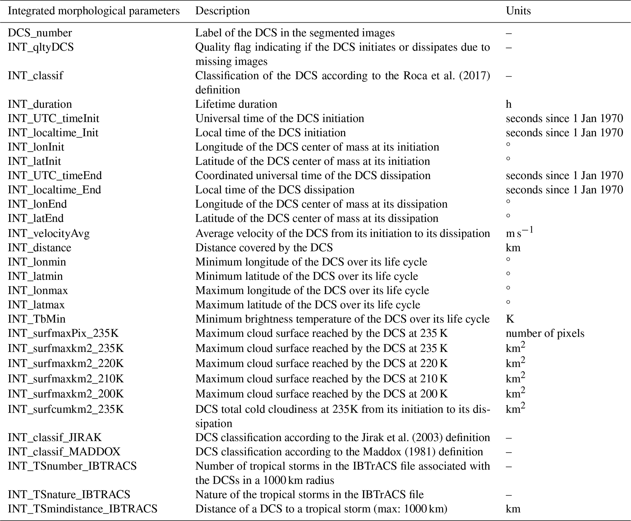
Table B2Morphological parameters described every 30 min over the life cycles of each deep convective system documented in the TOOCAN NetCDF4 and ASCII monthly tracking files.
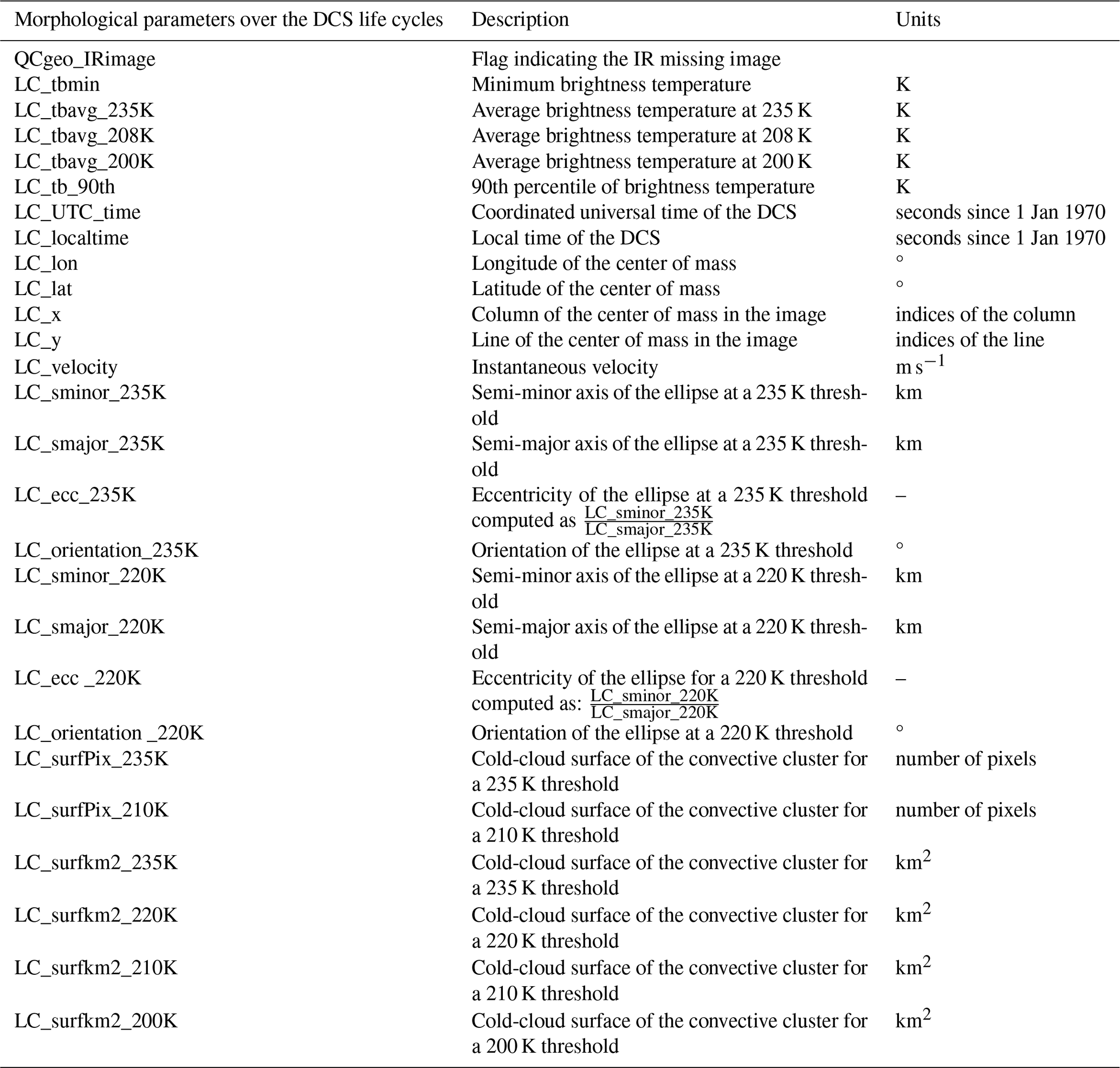
Table C1Morphological parameters of each DCS gridded into a 1° × 1° daily grid of the CACATOES netCDF-4 monthly files.
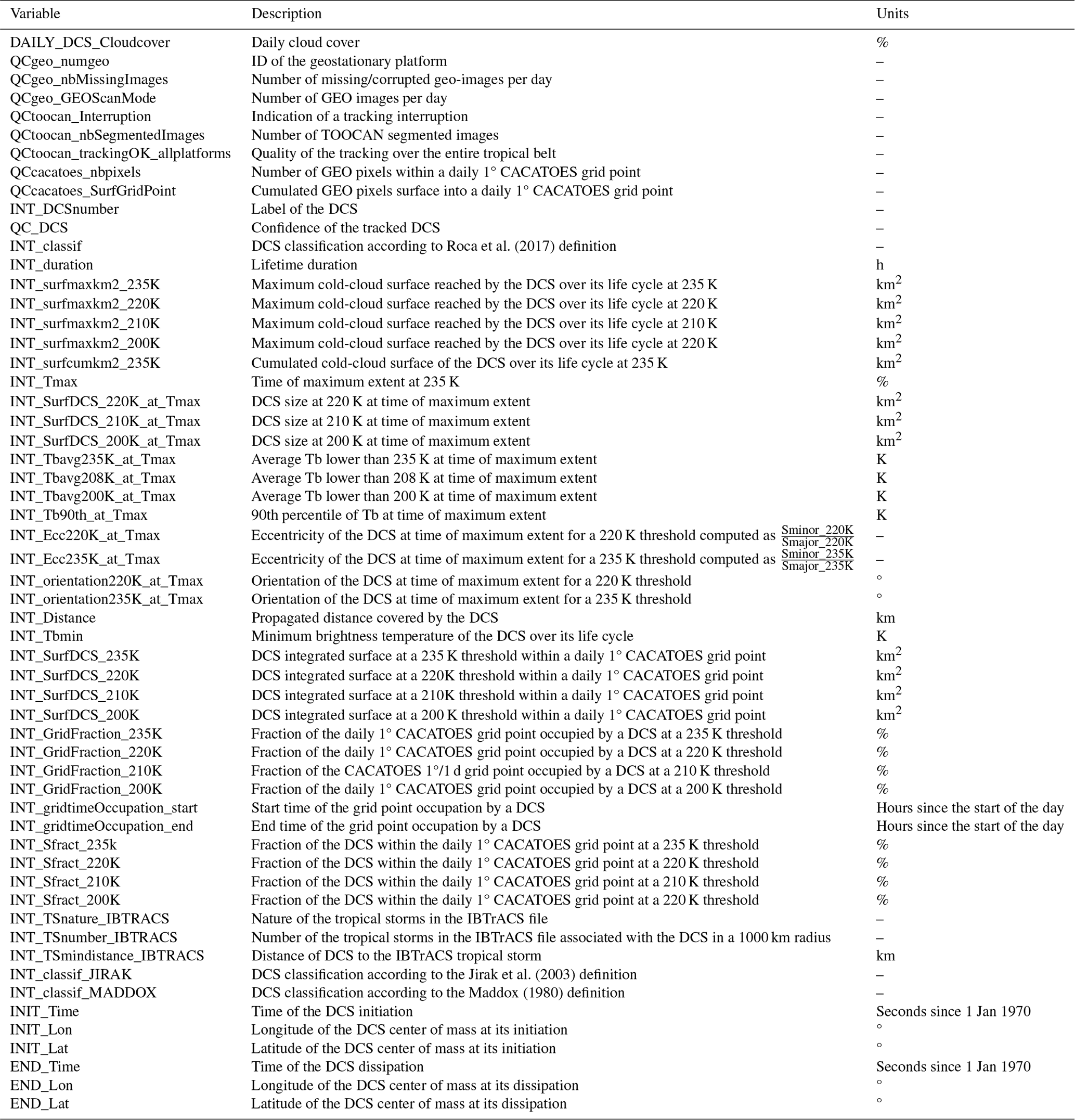
Video S1 (https://doi.org/10.5446/68200, Fiolleau, 2024) shows an animation of the convective situation segmented by TOOCAN from HIMAWARI IR data over the western Pacific region in October 2015.
TF and RR initiated the work. TF and RR prepared some datasets. TF drafted the figures. All the authors contributed to the writing of the paper.
The contact author has declared that neither of the authors has any competing interests.
Publisher's note: Copernicus Publications remains neutral with regard to jurisdictional claims made in the text, published maps, institutional affiliations, or any other geographical representation in this paper. While Copernicus Publications makes every effort to include appropriate place names, the final responsibility lies with the authors.
This work has been supported by CNRS and CNES under the Megha-Tropiques program. We thank the ESPRI/IPSL team for providing the computing and storage resources. We thank the French data center AERIS – and, especially, Sophie Cloché – for the help accessing the data (GEOring, ScaRaB). The authors also thank Laurent Gouttesoulard for his help in handling the geostationary satellite data archive. The authors further acknowledge Michel Dejus, project manager at CNES, and his team for their help with the technical aspects of ScaRaB. The authors also which to thank Nuria Duran-Gomez and Rémi Jugier from Magellium for their contribution to the GEOring homogenization.
This research has been supported by the CNES (MEGHA-TROPIQUES).
This paper was edited by Tobias Gerken and reviewed by two anonymous referees.
Arkin, P. A.: The Relationship between Fractional Coverage of High Cloud and Rainfall Accumulations during GATE over the B-Scale Array, https://doi.org/10.1175/1520-0493(1979)107<1382:TRBFCO>2.0.CO;2, 1979.
Arnaud, Y., Desbois, M., and Maizi, J.: Automatic Tracking and Characterization of African Convective Systems on Meteosat Pictures, J. Appl. Meteor. Climatol, 31, 443–453, https://doi.org/10.1175/1520-0450(1992)031<0443:ATACOA>2.0.CO;2, 1992.
Autones, F. and Moisselin, J.-M.: Algorithm Theoretical Basis Document for “Rapid Development Thunderstorms” (RDT-PGE11 v3.0), Scientific documentation of SAF/NWC, code SAF/NWC/CDOP2/MFT/SCI/ATBD/11, 2013.
Bellerby, T., Hsu, K., and Sorooshian, S.: LMODEL: A Satellite Precipitation Methodology Using Cloud Development Modeling. Part I: Algorithm Construction and Calibration, J. Hydrometeorol., 10, 1081–1095, https://doi.org/10.1175/2009jhm1091.1, 2009.
Berthet, S., Roca, R., Duvel, J. P., and Fiolleau, T.: Subseasonal variability of mesoscale convective systems over the tropical northeastern Pacific, Q. J. Roy. Meteor. Soc., 143, 1086–1094, https://doi.org/10.1002/qj.2992, 2017.
Boer, E. R. and Ramanathan, V.: Lagrangian approach for deriving cloud characteristics from satellite observations and its implications to cloud parameterization, J. Geophys. Res.-Atmos., 102, 21383–21399, https://doi.org/10.1029/97JD00930, 1997.
Bouniol, D., Roca, R., Fiolleau, T., and Poan, D. E.: Macrophysical, Microphysical, and Radiative Properties of Tropical Mesoscale Convective Systems over Their Life Cycle, J. Climate, 29, 3353–3371, https://doi.org/10.1175/jcli-d-15-0551.1, 2016.
Bouniol, D., Roca, R., Fiolleau, T., and Raberanto, P.: Life cycle-resolved observation of radiative properties of mesoscale convective systems, J. Appl. Meteorol. Climatol., 60, 1091–1104, https://doi.org/10.1175/JAMC-D-20-0244.1, 2021.
Carvalho, L. M. V. and Jones, C.: A Satellite Method to Identify Structural Properties of Mesoscale Convective Systems Based on the Maximum Spatial Correlation Tracking Technique (MASCOTTE), J. Appl. Meteorol., 40, 1683–1701, https://doi.org/10.1175/1520-0450(2001)040<1683:ASMTIS>2.0.CO;2, 2001.
Dias, J., Tulich, S. N., and Kiladis, G. N.: An Object-Based Approach to Assessing the Organization of Tropical Convection, J. Atmos. Sci., 69, 2488–2504, https://doi.org/10.1175/JAS-D-11-0293.1, 2012.
Elsaesser, G. S., Roca, R., Fiolleau, T., Del Genio, A. D., and Wu, J.: A Simple Model for Tropical Convective Cloud Shield Area Growth and Decay Rates Informed by Geostationary IR, GPM, and Aqua/AIRS Satellite Data, J. Geophys. Res.-Atmos., 127, e2021JD035599, https://doi.org/10.1029/2021JD035599, 2022.
Endlich, R. M. and Wolf, D. E.: Automatic Cloud Tracking Applied to GOES and METEOSAT Observations, J. Appl. Meteorol. Climatol., 20, 309–319, https://doi.org/10.1175/1520-0450(1981)020<0309:ACTATG>2.0.CO;2, 1981.
Esmaili, R. B., Tian, Y., Vila, D. A., and Kim, K. M.: A lagrangian analysis of cold cloud clusters and their life cycles with satellite observations, J. Geophys. Res., 121, 11723–11738, https://doi.org/10.1002/2016JD025653, 2016.
Evans, J. L. and Shemo, R. E.: A Procedure for Automated Satellite-Based Identification and Climatology Development of Various Classes of Organized Convection, J. Appl. Meteorol. Climatol., 35, 638–652, https://doi.org/10.1175/1520-0450(1996)035<0638:APFASB>2.0.CO;2, 1996.
Feng, Z., Leung, L. R., Liu, N., Wang, J., Houze, R. A., Li, J., Hardin, J. C., Chen, D., and Guo, J.: A Global High-Resolution Mesoscale Convective System Database Using Satellite-Derived Cloud Tops, Surface Precipitation, and Tracking, J. Geophys. Res.-Atmos., 126, e2020JD034202, https://doi.org/10.1029/2020JD034202, 2021.
Feng, Z., Hardin, J., Barnes, H. C., Li, J., Leung, L. R., Varble, A., and Zhang, Z.: PyFLEXTRKR: a flexible feature tracking Python software for convective cloud analysis, Geosci. Model Dev., 16, 2753–2776, https://doi.org/10.5194/gmd-16-2753-2023, 2023.
Fiolleau, T.: Animation of convective situation segmented by TOOCAN from HIMAWARI IR data over the Western Pacific region in October 2015, TIB AV Portal [video], https://doi.org/10.5446/68200, 2024.
Fiolleau, T. and Roca, R.: An algorithm for the detection and tracking of tropical mesoscale convective systems using infrared images from geostationary satellite, IEEE T. Geosci. Remote, 51, 4302–4315, https://doi.org/10.1109/TGRS.2012.2227762, 2013a.
Fiolleau, T. and Roca, R.: Composite life cycle of tropical mesoscale convective systems from geostationary and low Earth orbit satellite observations: method and sampling considerations, Q. J. Roy. Meteor. Soc., 139, 941–953, https://doi.org/10.1002/qj.2174, 2013b.
Fiolleau, T. and Roca, R.: TOOCAN Database V2.08 – Tracking Of Organized Convection Algorithm using a 3-dimensional segmentation, IPSL Data Catalog [data set], https://doi.org/10.14768/1be7fd53-8b81-416e-90d5-002b36b30cf8, 2023a.
Fiolleau, T. and Roca, R.: CACATOES database V1.04, IPSL Data Catalog [data set], https://doi.org/10.14768/98569eea-d056-412d-9f52-73ea07b9cdca, 2023b.
Fiolleau, T. and Roca, R.: GEOgrid_coldcloud: a 2012–2020 global homogenized infrared dataset from a fleet of geostationary satellites, IPSL Data Catalog [data set], https://doi.org/10.14768/93f138f5-a553-4691-96ed-952fd32d2fc3, 2023c.
Fiolleau, T., Roca, R., Cloche, S., Bouniol, D., and Raberanto, P.: Homogenization of Geostationary Infrared Imager Channels for Cold Cloud Studies Using Megha-Tropiques/ScaRaB, IEEE T. Geosci. Remote, 58, 6609–6622, https://doi.org/10.1109/TGRS.2020.2978171, 2020.
Guilloteau, C. and Foufoula-Georgiou, E.: Life Cycle of Precipitating Cloud Systems from Synergistic Satellite Observations: Evolution of Macrophysical Properties and Precipitation Statistics from Geostationary Cloud tracking and GPM Active and Passive Microwave Measurements, J. Hydrometeorol., https://doi.org/10.1175/jhm-d-23-0185.1, 2024.
Harper, B., Kepert, J., and Ginger, J.: Wind speed time averaging conversions for tropical cyclone conditions, in: Proc. 28th Conference Hurricanes and Tropical Meteorology (AMS, 2008), 27 April–2 May 2008, Palms Foyer, USA, 2008.
Heikenfeld, M., Marinescu, P. J., Christensen, M., Watson-Parris, D., Senf, F., van den Heever, S. C., and Stier, P.: tobac 1.2: towards a flexible framework for tracking and analysis of clouds in diverse datasets, Geosci. Model Dev., 12, 4551–4570, https://doi.org/10.5194/gmd-12-4551-2019, 2019.
Hennon, C. C., Helms, C. N., Knapp, K. R., and Bowen, A. R.: An objective algorithm for detecting and tracking tropical cloud clusters: Implications for tropical cyclogenesis prediction, J. Atmos. Ocean. Tech., 28, 1007–1018, https://doi.org/10.1175/2010JTECHA1522.1, 2011.
Hennon, C. C., Papin, P. P., Zarzar, C. M., Michael, J. R., Adam Caudill, J., Douglas, C. R., Groetsema, W. C., Lacy, J. H., Maye, Z. D., Reid, J. L., Scales, M. A., Talley, M. D., and Helms, C. N.: Tropical cloud cluster climatology, variability, and genesis productivity, J. Climate, 26, 3046–3066, https://doi.org/10.1175/JCLI-D-12-00387.1, 2013.
Hewison, T. J., Wu, X., Yu, F., Tahara, Y., Hu, X., Kim, D., and Koenig, M.: GSICS inter-calibration of infrared channels of geostationary imagers using metop/IASI, IEEE T. Geosci. Remote, 51, 1160–1170, https://doi.org/10.1109/TGRS.2013.2238544, 2013.
Hodges, K. I.: A General-Method For Tracking Analysis And Its Application To Meteorological Data, Mon. Weather Rev., 122, 2573–2586, https://doi.org/10.1175/1520-0493(1994)122<2573:AGMFTA>2.0.CO;2, 1994.
Houze Jr., R. A.: Mesoscale Convective Systems, Rev. Geophys., 42, 1–43, https://doi.org/10.1029/2004RG000150, 2004.
Houze, R. A.: 100 Years of Research on Mesoscale Convective Systems, Meteorological Monographs, AMSMONOGRAPHS-D-18-0001.1, https://doi.org/10.1175/AMSMONOGRAPHS-D-18-0001.1, 2018.
Huang, X., Hu, C., Huang, X., Chu, Y., Tseng, Y., Zhang, G. J., and Lin, Y.: A long-term tropical mesoscale convective systems dataset based on a novel objective automatic tracking algorithm, Clim. Dynam., 51, 3145–3159, https://doi.org/10.1007/s00382-018-4071-0, 2018.
Jirak, I. L., Cotton, W. R., and Mcanelly, R. L.: Satellite and Radar Survey of Mesoscale Convective System Development, Mon. Weather Rev., 131, 2428–2449, https://doi.org/10.1175/1520-0493(2003)131<2428:SARSOM>2.0.CO;2, 2003.
Jones, W. K., Christensen, M. W., and Stier, P.: A semi-Lagrangian method for detecting and tracking deep convective clouds in geostationary satellite observations, Atmos. Meas. Tech., 16, 1043–1059, https://doi.org/10.5194/amt-16-1043-2023, 2023.
Knapp, K. R., Kruk, M. C., Levinson, D. H., Diamond, H. J., and Neumann, C. J.: The international best track archive for climate stewardship (IBTrACS), B. Am. Meteorol. Soc., 91, 363–376, https://doi.org/10.1175/2009BAMS2755.1, 2010.
Knapp, K. R., Ansari, S., Bain, C. L., Bourassa, M. A., Dickinson, M. J., Funk, C., Helms, C. N., Hennon, C. C., Holmes, C. D., Huffman, G. J., Kossin, J. P., Lee, H. T., Loew, A., and Magnusdottir, G.: Globally Gridded Satellite observations for climate studies, B. Am. Meteorol. Soc., 92, 893–907, https://doi.org/10.1175/2011BAMS3039.1, 2011.
Kruk, M. C., Knapp, K. R., and Levinson, D. H.: A technique for combining global tropical cyclone best track data, J. Atmos. Ocean. Tech., 27, 680–692, https://doi.org/10.1175/2009JTECHA1627.1, 2010.
Laing, A. G. and Fritsch, J. M.: The global population of mesoscale convective complexes, Q. J. Roy. Meteor. Soc., 123, 389–405, https://doi.org/10.1002/qj.49712353807, 1997.
Laing, A. G. and Fritsch, J. M.: The Large-Scale Environments of the Global Populations of Mesoscale Convective Complexes, Mon. Weather Rev., 128, 2756–2776, 2000.
Liu, C., Zipser, E. J., and Nesbitt, S. W.: Global Distribution of Tropical Deep Convection: Different Perspectives from TRMM Infrared and Radar Data, J. Climate, 20, 489–503, https://doi.org/10.1175/jcli4023.1, 2007.
Liu, C., Zipser, E. J., Cecil, D. J., Nesbitt, S. W., and Sherwood, S.: A cloud and precipitation feature database from nine years of TRMM observations, J. Appl. Meteorol. Climatol., 47, 2712–2728, https://doi.org/10.1175/2008JAMC1890.1, 2008.
Machado, L. A. T. and Rossow, W. B.: Structural Characteristics and Radiative Properties of Tropical Cloud Clusters, Mon. Weather Rev., 121, 3234–3260, https://doi.org/10.1175/1520-0493(1993)121<3234:SCARPO>2.0.CO;2, 1993.
Machado, L. A. T., Desbois, M., Duvel, J.-P., Machado, L. A. T., Desbois, M., and Duvel, J.-P.: Structural Characteristics of Deep Convective Systems over Tropical Africa and the Atlantic Ocean, Mont. Weather Rev., 120, 392–406, https://doi.org/10.1175/1520-0493(1992)120<0392:SCODCS>2.0.CO;2, 1992.
Machado, L. A. T., Rossow, W. B., Guedes, R. L., and Walker, A. W.: Life Cycle Variations of Mesoscale Convective Systems over the Americas, Mon. Weather Rev., 126, 1630–1654, 1998.
Maddox, R. A.: Mesoscale Convective Complexes, B. Am. Meteorol. Soc., 61, 1374–1387, 1980.
Mapes, B. and Houze, R. A.: Cloud Clusters and Superclusters over the Oceanic Warm Pool, Mon. Weather Rev., 121, 1398–1415, https://doi.org/10.1175/1520-0493(1993)121<1398:CCASOT>2.0.CO;2, 1993.
Mapes, B., Milliff, R., and Morzel, J.: Composite life cycle of maritime tropical mesoscale convective systems in scatterometer and microwave satellite observations, J. Atmos. Sci., 66, 199–208, https://doi.org/10.1175/2008JAS2746.1, 2009.
Mathon, V. and Laurent, H.: Life cycle of Sahelian mesoscale convective cloud systems, Q. J. Roy., Meteor. Soc., 127, 377–406, https://doi.org/10.1002/qj.49712757208, 2001.
Mohr, K. I. and Zipser, E. J.: Mesoscale Convective Systems Defined by Their 85-GHz Ice Scattering Signature: Size and Intensity Comparison over Tropical Oceans and Continents, Mon. Weather Rev., 124, 2417–2437, https://doi.org/10.1175/1520-0493(1996)124<2417:mcsdbt>2.0.co;2, 1996.
Ocasio, K. M. N., Evans, J. L., and Young, G. S.: Tracking mesoscale convective systems that are potential candidates for tropical cyclogenesis, Mon. Weather Rev., 148, 655–669, https://doi.org/10.1175/MWR-D-19-0070.1, 2020.
Ostlund, S.: Computer Software for Rainfall Analyses and Echo Tracking of Digitized Radar Data, NOAA technical memorandum ERL WMPO, 15, 1974.
Poujol, B., Prein, A. F., and Newman, A. J.: Kilometer-scale modeling projects a tripling of Alaskan convective storms in future climate, Clim. Dynam., 55, 3543–3564, https://doi.org/10.1007/s00382-020-05466-1, 2020.
Prein, A. F., Feng, Z., Fiolleau, T., Moon, Z. L., Núñez Ocasio, K. M., Kukulies, J., Roca, R., Varble, A. C., Rehbein, A., Liu, C., Ikeda, K., Mu, Y., and Rasmussen, R. M.: Km-Scale Simulations of Mesoscale Convective Systems Over South America – A Feature Tracker Intercomparison, J. Geophys. Res.-Atmos., 129, e2023JD040254, https://doi.org/10.1029/2023JD040254, 2024.
Rajagopal, M., Russell, J., Skok, G., and Zipser, E.: Tracking Mesoscale Convective Systems in IMERG and Regional Variability of Their Properties in the Tropics, J. Geophys. Res.-Atmos., 128, e2023JD038563, https://doi.org/10.1029/2023JD038563, 2023.
Roca, R. and Fiolleau, T.: Extreme precipitation in the tropics is closely associated with long-lived convective systems, Commun. Earth Environ., 1, 18, https://doi.org/10.1038/s43247-020-00015-4, 2020.
Roca, R. and Ramanathan, V.: Scale dependence of monsoonal convective systems over the Indian Ocean, J. Climate, 13, 1286–1298, https://doi.org/10.1175/1520-0442(2000)013<1286:SDOMCS>2.0.CO;2, 2000.
Roca, R., Berges, J. C., Brogniez, H., Capderou, M., Chambon, P., Chomette, O., Cloche, S., Fiolleau, T., Jobard, I., and Lemond, J.: On the water and energy cycles in the Tropics, Comptes Rendus Geosciences, 342, 390–402, https://doi.org/10.1016/j.crte.2010.01.003, 2010.
Roca, R., Aublanc, J., Chambon, P., Fiolleau, T., and Viltard, N.: Robust observational quantification of the contribution of mesoscale convective systems to rainfall in the tropics, J. Climate, 27, 4952–4958, https://doi.org/10.1175/JCLI-D-13-00628.1, 2014.
Roca, R., Fiolleau, T., and Bouniol, D.: A simple model of the life cycle of mesoscale convective systems cloud shield in the tropics, J. Climate, 30, 4283–4298, https://doi.org/10.1175/JCLI-D-16-0556.1, 2017.
Roca, R., Bouniol, D., and Fiolleau, T.: On the Duration and Life Cycle of Precipitation Systems in the Tropics, in: Satellite Precipitation Measurement: Volume 2, edited by: Levizzani, V., Kidd, C., Kirschbaum, D., Kummerow, C., Nakamura, K., and Turk, F., Springer International Publishing, Cham, 729–744, https://doi.org/10.1007/978-3-030-35798-6_14, 2020.
Roca, R., Fiolleau, T., Viju, J., and Schulz, J.: METEOSAT Long-Term Observations Reveal Changes in Convective organization over Tropical Africa and Atlantic Ocean, Surv. Geophys., in review, 2024.
Schröder, M., König, M., and Schmetz, J.: Deep convection observed by the Spinning Enhanced Visible and Infrared Imager on board Meteosat 8: Spatial distribution and temporal evolution over Africa in summer and winter 2006, J. Geophys. Res.-Atmos., 114, 1–14, https://doi.org/10.1029/2008JD010653, 2009.
Szantai, A., Six, B., Cloché, S., and Sèze, G.: megha-tropiques MTTM Megha-Tropiques Technical Memorandum Quality of geostationary satellite images Megha-Tropiques Quality of geostationary satellite images, https://meghatropiques.ipsl.fr/download/megha-tropiques-technical-memorandum-n3/ (last access: 9 September 2024), 2011.
Tan, J., Jakob, C., Rossow, W. B., and Tselioudis, G.: Increases in tropical rainfall driven by changes in frequency of organized deep convection, Nature, 519, 451–454, https://doi.org/10.1038/nature14339, 2015.
Tsakraklides, G. and Evans, J. L.: Global and regional diurnal variations of organized convection, J. Climate, 16, 1562–1572, https://doi.org/10.1175/1520-0442-16.10.1562, 2003.
Vant-Hull, B., Rossow, W., and Pearl, C.: American Meteorological Society Global Comparisons of Regional Life Cycle Properties and Motion of Multiday Convective Systems: Tropical and Midlatitude Land and Ocean, J. Climate, 29, 5837–5858, https://doi.org/10.1175/JCLI-D-15-0698.1, 2016.
Wilcox, E. M.: Spatial and temporal scales of precipitating tropical cloud systems in satellite imagery and the NCAR CCM3, J. Climate, 16, 3545–3559, https://doi.org/10.1175/1520-0442(2003)016<3545:SATSOP>2.0.CO;2, 2003.
Williams, M. and Houze, R. A.: Satellite-Observed Characteristics of Winter Monsoon Cloud Clusters, Mon. Weather Rev., 115, 505–519, https://doi.org/10.1175/1520-0493(1987)115<0505:SOCOWM>2.0.CO;2, 1987.
WMO: Measurement of surface wind. Guide to Meteorological Instruments and Methods of Observations, 5th edn., World Meteorological Organization Tech. Rep. WMO-8, 1983.
Woodley, W. L., Griffith, C. G., Griffin, J. S., and Stromatt, S. C.: The Inference of GATE Convective Rainfall from SMS-1 Imagery, J. Appl. Meteorol., 19, 388–408, 1980.
GEOring refers to the entirety of the geostationary platforms whose data, all together, cover the entire longitude of the Earth's surface.