Time series of alpine snow surface radiative-temperature maps from high-precision thermal-infrared imaging

The surface temperature of snow cover is a key variable, as it provides information about the current state of the snowpack, helps predict its future evolution, and enhances estimations of the snow water equivalent. Although satellites are often used to measure the surface temperature despite the difficulty of retrieving accurate surface temperatures from space, calibration–validation datasets over snow-covered areas are scarce. We present a dataset of extensive measurements of the surface radiative temperature of snow acquired with an uncooled thermal-infrared (TIR) camera. The set accuracy goal is 0.7 K, which is the radiometric accuracy of the TIR sensor of the future CNES/ISRO TRISHNA mission. TIR images have been acquired over two winter seasons, November 2021 to May 2022 and February to May 2023, at the Col du Lautaret, 2057 m a.s.l. in the French Alps. During the first season, the camera operated in the off-the-shelf configuration with rough thermal regulation (7–39 °C). An improved setup with a stabilized internal temperature was developed for the second campaign, and comprehensive laboratory experiments were carried out in order to characterize the physical properties of the components of the TIR camera and its calibration. Thorough processing, including radiometric processing, orthorectification, and a filter for poor-visibility conditions due to fog or snowfall, was performed. The result is two winter season time series of 130 019 maps of the surface radiative temperature of snow with meter-scale resolution over an area of 0.5 km². The validation was performed against precision TIR radiometers. We found an absolute accuracy (mean absolute error, MAE) of 1.28 K during winter 2021–2022 and 0.67 K for spring 2023. The efforts to stabilize the internal temperature of the TIR camera therefore led to a notable improvement of the accuracy. Although some uncertainties persist, particularly the temperature overestimation during melt, this dataset represents a major advance in the capacity to monitor and map surface temperature in mountainous areas and to calibrate–validate satellite measurements over snow-covered areas of complex topography. The complete dataset is provided at https://doi.org/10.57932/8ed8f0b2-e6ae-4d64-97e5-1ae23e8b97b1 (Arioli et al., 2024a) and https://doi.org/10.57932/1e9ff61f-1f06-48ae-92d9-6e1f7df8ad8c (Arioli et al., 2024b).

1 Introduction

Snow is a crucial element of alpine ecosystems, as its high reflectivity cools the climate of high-altitude environments, while its insulating properties contribute to the preservation of glaciers (Barry, 2002). In alpine areas, it represents a crucial water storage medium for downstream ecosystems and human populations (Grabherr et al., 2010). Indeed, with over one-sixth of the world population relying on the high-mountain cryosphere as a water supply (Barnett et al., 2005), extensive monitoring of the snowpack is key to improving the understanding of future changes in water resources (Fayad et al., 2017; Beniston et al., 2018).

The surface temperature of snow is one of the key variables used to monitor the status of the snowpack. It plays a major role in the surface energy budget, which describes the exchanges of energy between the snowpack and the atmosphere (Armstrong and Brun, 2008); it provides insights about the onset and duration of surface melt (Alonso-González et al., 2023); and it influences the evolution of the microstructural and optical properties of the snow grains (Colbeck, 1989; Flanner and Zender, 2006). However, surface temperature variations are difficult to capture and predict. Indeed, due to the insulating properties of snow, its thermal inertia is low, allowing minute-scale changes of the surface temperature. Furthermore, in mountainous areas, it shows large variation spatially at meter and longer scales because of the complex terrain (Lundquist and Cayan, 2007). Indeed, phenomena such as (1) a variable illumination intensity according to the surface slope and orientation, (2) the reflection of sunlight and emission of thermal-infrared radiation towards neighboring slopes, and (3) variations of the air temperature with altitude due to the lapse rate and atmospheric turbulence induce large spatial variations in the local surface energy budget (Fierz et al., 2003; Adams et al., 2011; Robledano et al., 2022).

Thermal-infrared (TIR) sensors on board satellites and other spatial platforms, such as NASA's Landsat 8/9 TIRS/2, ECOSTRESS, ASTER, and NOAA's AVHRR, monitor the surface temperatures of snow-covered areas extensively and regularly (Roy, 2014; Hook and Hulley, 2019; Hulley and Hook, 2010; Kerr et al., 1992). Over mountainous terrain, however, the resolution of most sensors, which is on the order of 100 m to 1 km, is coarse with respect to the spatial temperature variations within a single pixel, leading to higher measurement uncertainty (Hall et al., 2008; Simó et al., 2016; He et al., 2019). Also, the revisit time of the TIR sensors currently in orbit, which is on the order of half a day for sensors with 1 km resolution and up to 16 d for ASTER (with 90 m resolution), combined with the intermittency of cloud cover makes the temporal distance between successive useful clear-sky images significantly larger than the typical timescales of surface temperature variation (Wang et al., 2001). A new generation of thermal-infrared sensors are to be launched between 2026 and 2030 on board the TRISHNA, LSTM, and SBG satellites (Buffet et al., 2021; Bernard et al., 2023; Stavros et al., 2023). These sensors will have enhanced resolutions of between 50 and 70 m and revisit times of ≤3 d individually and 1 d when combined (day pass). They will therefore significantly increase the amount of high-resolution thermal data available over terrestrial surfaces, improving the current understanding of the snow surface energy budget and the estimation of water resources in Alpine areas and cold regions (Alonso-González et al., 2023). However, some difficulties inherent to remote measurements in mountainous areas remain to be solved. Indeed, most atmospheric correction algorithms of satellite images only partially account for the underlying topography (Zhu et al., 2020). Additionally, how the sub-pixel variability of the snow surface temperature affects satellite measurements is still unclear. These uncertainties result from the scarcity of calibration–validation initiatives for thermal-infrared acquisition over snow-covered areas (Dybkjær et al., 2012; Høyer et al., 2017). In addition, because of its extent and its well-known temperature of 0 °C during the melting season, snow is an interesting material for the scope of calibration–validation.

Recently, uncooled thermal-infrared cameras have become an affordable means to perform high-resolution and high-revisit-time measurements of the surface temperature, similarly to webcams. However, their use has been limited by multiple instrumental biases that make these instruments far from an off-the-shelf solution for scientific applications requiring high accuracy (Aasen et al., 2018). Indeed, measurements are extremely sensitive to the temperature of the sensor itself and that of the camera body (Budzier and Gerlach, 2015) and the instrument response drifts over time (Olbrycht et al., 2012). This causes offsets of several K in the measured temperature and creates artifacts in the image (Riou et al., 2004). Many of these issues are partially corrected by flat-field correction (FFC). During FFC, a shutter of known temperature and emissivity is regularly measured by the sensor. The offset between the measurement and the real shutter temperature is then applied to the following measurements pixel by pixel, compensating for the errors that build up during operation (Nugent et al., 2013; Virtue et al., 2021). FFC is typically applied every few seconds to every few minutes. Still, even with an FFC system, most manufacturers' declared accuracies of TIR cameras range between 2 and 5 K (Kelly et al., 2019). This is insufficient for the purpose of TIR satellite calibration–validation, considering that most spaceborne TIR sensors have a radiometric accuracy between 0.1 and 0.8 K (Barsi et al., 2014; Smith et al., 2020; Smyth and Logan, 2022). As a result, attempts to acquire thermal imagery on snow surfaces are scarce in the scientific literature and mainly focus on temperature anomalies rather than on the absolute surface temperature (Shea et al., 2012; Kraaijenbrink et al., 2018; Wigmore and Molotch, 2023).

This study presents observations of the surface temperature over two winter seasons in an Alpine catchment with complex terrain (Col du Lautaret in the French Alps). The dataset includes high-frequency (2 min) time series of images of the surface temperature acquired with an uncooled TIR camera. The particularity of this dataset is the high quality of the calibration and stabilization of the camera and the availability of ancillary measurements to perform a precise cross-evaluation with the aim of achieving high accuracy. The accuracy goal fixed for the dataset is 0.7 K, which is the radiometric accuracy expected for the TRISHNA satellite, which carries the precursor of the new generation of TIR imaging radiometers. This paper describes the thorough step-by-step processing of raw data and the careful assessment of the measurement uncertainty. During processing, snow is treated as a black body. While the actual emissivity of snow is between 0.96 and 0.99 at nadir (Hori et al., 2006), choosing a precise value for the snow emissivity is challenging because of its potential variations with grain type and the presence of surface water during the melting season (Dozier and Warren, 1982; Hori et al., 2014). Other in situ measurements include snow surface temperatures from TIR radiometers deployed in the camera's field of view (FOV) – used as ground truth; RGB images of the scene; time series of the internal temperature of the TIR camera; and meteorological parameters that are helpful for the interpretation of the camera measurements, such as incoming longwave radiation, air temperature and humidity, and wind speed. The study site is described in Sect. 2. The instruments used, the lab characterization of the TIR camera, and the processing of the measurements are described in Sects. 3, 4, and 5, respectively. The results are presented in Sect. 6, validated in Sect. 7, and discussed in Sect. 8.

2 Study site

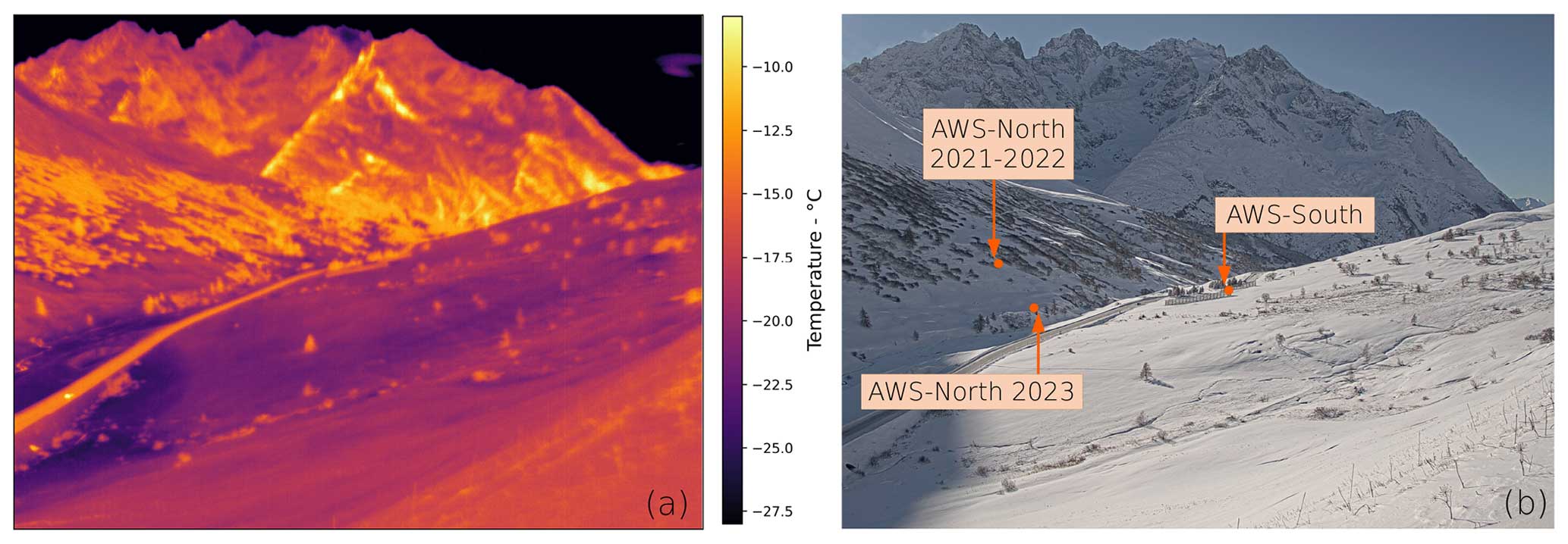
The two winter measurement campaigns took place at the Col du Lautaret site in the French Alps (Fig. 1, 45.0347° N, 6.4051° E), at an altitude of 2057 m a.s.l. The imaged site is located next to the Col du Lautaret pass, with the TIR camera pointing west. It includes a north-facing slope (Fig. 2, left) and a south-facing slope (Fig. 2, right) and spans altitudes between 1950 and 2200 m. The Meije massif in the Écrins mountain range is visible in the background. South of the col, the relief steeply climbs above 3000 m, masking sunlight from the north-facing slope of the pass during most of winter. On the other hand, the south-facing slope receives at least some sunlight every day. Snow covers the soil between approximately December and April every winter, with very high spatial variability in snow depth. Advanced meteorological parameters are measured continuously at the Fluxalp ICOS station 500 m north of the col and are available via open access (https://meta.icos-cp.eu/resources/stations/ES_FR-CLt, last access: 14 August 2024).

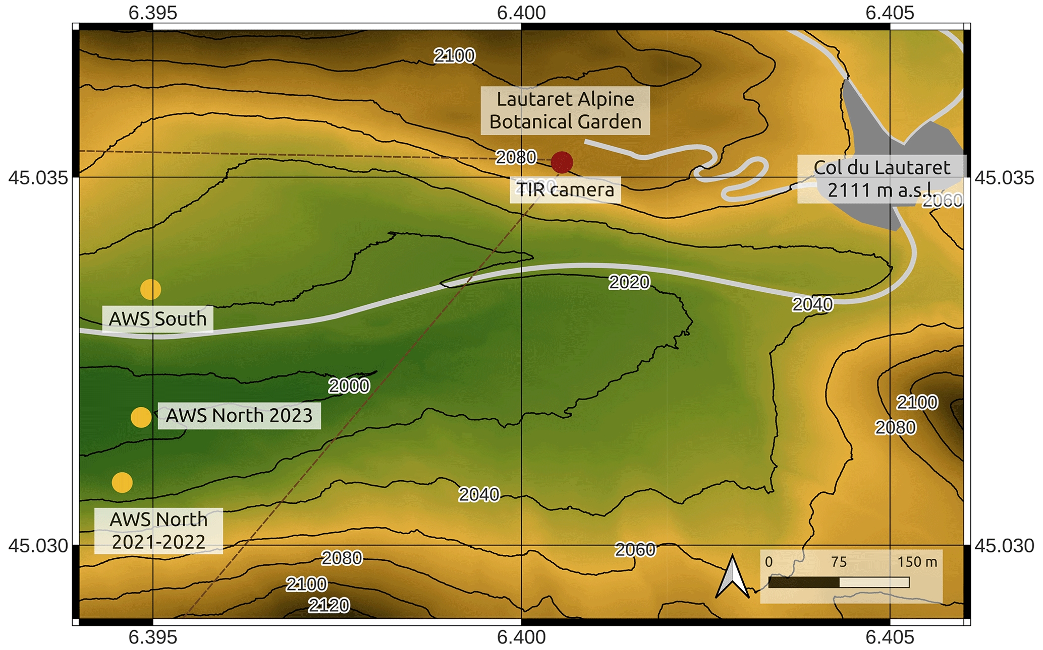
Figure 1 Map of the west side of the Col du Lautaret, France (45.0347° N, 6.4051° E) showing the location of the TIR camera, its field of view, and two automatic weather stations deployed on the north and south faces. AWS-North was relocated between winter 2021–2022 and spring 2023.

Figure 2 Photographs taken by the TIR camera (a) and a standard RGB camera (b).

3 Instruments

3.1 Thermal-infrared camera

The time series of surface temperature images are acquired using an Optris Pi640 camera. Its sensor consists of a focal plane array of 640 × 480 microbolometers that measure the incoming radiance in the thermal-infrared domain between 8 and 14 µm (Optris, 2020). Microbolometers work at ambient temperature and therefore do not require expensive cooling systems. However, their response is unstable over time and particularly sensitive to environmental temperature changes. To compensate for these two sources of uncertainty, the camera comes with an internal shutter system to perform FFC. Besides its radiometric utility, FFC also reduces noise across the image. The FFC process is controlled by the camera software. In addition, the camera is enclosed in an aluminum casing with a basic thermal regulation system (between 10 and 30 °C). The conversion of the signal from digital numbers to temperature is also performed by the camera software. The measurement output is an array of 640 × 480 temperatures at a resolution of 0.1 K, recorded as a comma-separated value (csv) file. We configured the acquisition to occur every 2 min during field campaigns.

This off-the-shelf setup of the TIR camera was used for the whole 2021–2022 winter campaign between November 2021 and May 2022. However, we identified that the large internal fluctuations of temperature jeopardized our goal in terms of accuracy. For spring 2023, the setup was therefore modified. The camera was isolated inside the original casing by placing it in a small enclosure whose temperature was kept close to constant (<2 K fluctuation) by a thermoelectric module (TEM), while the rest of the casing was used to evacuate the heat excess (Fig. 3a). The volume with the camera and the rest of the casing was ventilated to keep the temperature uniform inside. Because of the limited power of the TEM, the presence of active electronics inside the camera body, and wide external temperature variations, the internal temperature was typically between −0.5 to +1.0 K with respect to the TEM settings used during operation, but it varied slowly over time.

The camera in its casing, paired with a waterproof box containing both the camera and the TEM electronics, was installed on the south wall of the museum building of the Lautaret Garden (6.4006° E, 45.0352° N; Fig. 3b). A small wooden roof was installed on top of the camera to avoid overheating due to direct exposure to sunlight and the accumulation of snowfall. The internal temperature of the camera was initially set to 15 °C. However, this temperature proved to be too low with respect to the limited heat evacuation in the rear of the casing of this setup, causing significant overheating when the external temperature approached 15 °C. It was then raised to 22 °C on the 17 February 2023 after several episodes of overheating during the first week of measurements. By raising the TEM setting temperature from 15 to 22 °C, the required heat evacuation was reduced and no overheating episodes happened during the rest of the season.

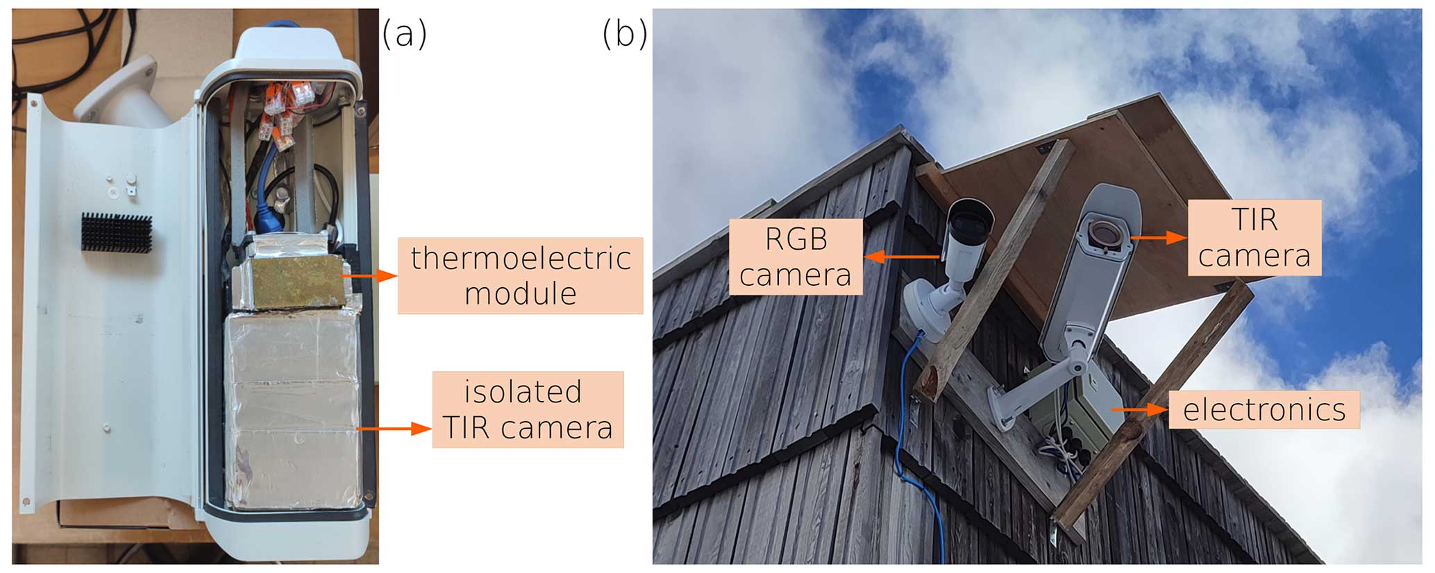
Figure 3 The interior of the Optris Pi640 TIR camera's casing in the spring 2023 setup. (a) The camera is isolated in the volume below, while the TEM and radiators for heat evacuation are on top. (b) The TIR camera (on the right) and a regular RGB camera (Axis P1448-LE; on the left) under the protective roof.

3.2 Other instruments

3.2.1 Visible camera

An RGB camera (Axis P1448-LE) was mounted to the side of the TIR camera (Fig. 3b). The fields of view (FOVs) of the two cameras corresponded approximately (Fig. 2). Visible images were acquired every 10 min during operation of the TIR camera and were used to support the visualization and interpretation of the lower-resolution TIR images, especially during foggy or snowy conditions.

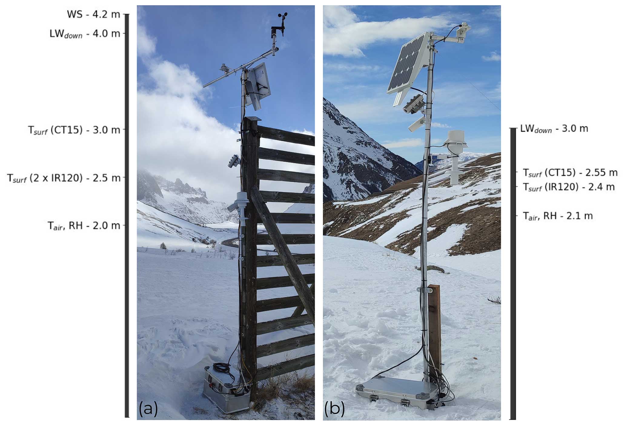
3.2.2 Automatic weather stations

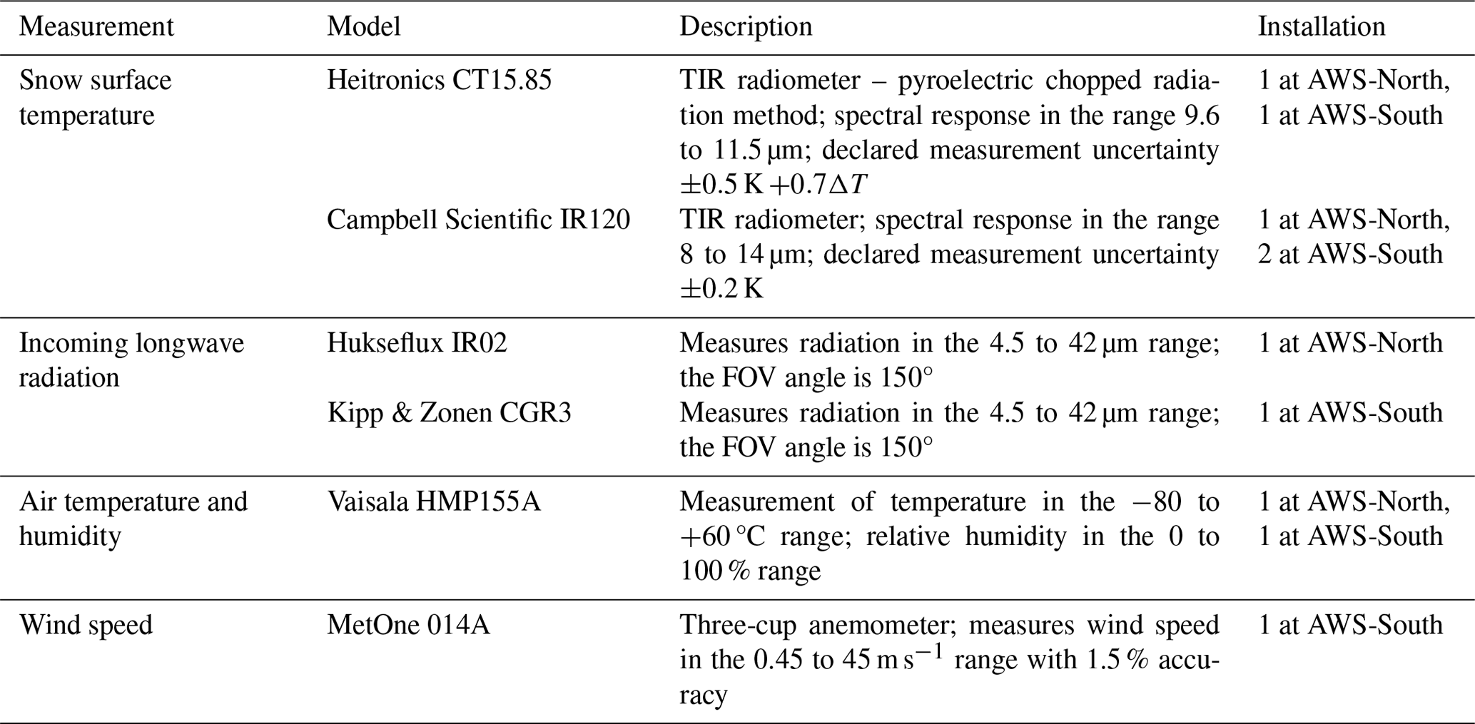
During winter 2021–2022, three Campbell Scientific IR120 TIR radiometers were installed in the camera's FOV, two on the south-facing and one on the north-facing slope (Figs. 1 and 2). During spring 2023, the three radiometers used during the previous season were integrated into two more complete automatic weather stations (AWSs), one situated on the north-facing slope (AWS-North) and one on the south-facing slope (AWS-South; Figs. 1 and 2). The list of measurements performed and the instruments employed are described in Table 1, while their setup is illustrated in Fig. 4. TIR radiometer measurements were used as ground truth to validate the TIR camera measurements. During the second campaign, two high-precision Heitronics CT15.85 radiometers were added to the three Campbell Scientific IR120 radiometers used during the first campaign after noticing a warm error from the IR120 sensors of up to 1.7 K over melting snow. While these sensors proved to be very precise in controlled laboratory conditions, they are sensitive to changes to the sensor temperature that occur in the field, resulting in a degraded accuracy. The Heitronics radiometers compensate for this effect with a re-calibration that is performed every 10 s approximately.

Table 1 List of measurements performed and basic specifications of the instruments installed at AWS-North and AWS-South at the Col du Lautaret site.

Figure 4 Photograph and scheme of the instrument setup at AWS-South (a) and AWS-North (b).

3.3 Other measurements

Ground control points (GCPs), i.e., points with well-known locations in both the TIR camera and world coordinates, were acquired regularly throughout the two seasons. They were obtained as follows. A 100 × 70 cm aluminum plate was displaced across the camera's FOV. At specific locations, the plate was laid on the ground and an RTK-GPS (RTK signifies real-time kinematics) measurement of its position with 0.01 m accuracy was acquired. The aluminum plate has low emissivity and only reflects the sky temperature, which is, in clear-sky conditions, much colder than the snow surface. The position of the aluminum plate during the GPS survey was therefore clearly distinguishable in the TIR images. Twenty-one GCPs were acquired during winter 2021–2022 and 25 during spring 2023. Their positions in both world and camera coordinates are listed in Tables A1 and A2 and are shown in Figs. A1 and A2 in Appendix A.

Also, the internal temperature of the TIR camera, T_int, was measured continuously and recorded every 2 s through the COM-port communication tool of the Optris PIX-Connect software (Optris, 2018).

4 TIR camera characterization

Between winter 2021–2022 and spring 2023 and after the instrument setup modification, some physical parameters of the TIR camera were measured during laboratory experiments, and its calibration was verified. The results of this characterization were used later to process the data acquired during the two field campaigns.

4.1 Assessment of the distortion parameters

An assessment of the distortion parameters of the TIR camera was performed using the calibrateCamera function of the OpenCV Python library (Itseez, 2015). More specifically, 55 TIR images of a chessboard taken in different directions and held in different orientations were acquired in the lab. The chessboard developed for this application had alternating wood (high emissivity) and aluminum (low emissivity) squares in order to enhance the contrast in front of the thermal sensor. During the acquisition, the internal temperature of the camera was set to +15 °C. The positions in the images of the chessboard corners were recognized by the findChessboardCorners OpenCV function, and these positions were passed down to the calibrateCamera function, which computed the distortion parameters. The resulting radial distortion coefficients k_n and tangential distortion coefficients p_n were

$$\begin{array}{}\text{(1)}& \begin{array}{rl}{k}_{\mathrm{1}}& =-\mathrm{0.42230},k_{\mathrm{2}}=\mathrm{0.52240},k_{\mathrm{3}}=-\mathrm{0.64157},\\ & p_{\mathrm{1}}=\mathrm{0.00003},p_{\mathrm{2}}=\mathrm{0.00185}.\end{array}\end{array}$$

4.2 Determination of the camera window model

The camera was located inside an aluminum casing equipped with a germanium window coated with an anti-reflection film. Still, its transmissivity was slightly below 1, which meant that part of the signal measured by the TIR camera's sensor did not come from the target but was either (1) the thermal emission of the window towards the sensor, (2) the reflection of the casing's thermal emission onto the window, or (3) the combined effect of (1) and (2). Since the temperatures of both the casing and the window are significantly higher than the snow surface during use, even a small percentage of their emission can increase the measured temperature by many degrees. The manufacturer supplied a transmittivity value of 0.92 but no reflectivity or emissivity values. Moreover, we found this transmittivity to be lower than those of most germanium windows with an anti-reflection coating (0.95–0.99) available commercially. Also, atmospheric UV radiation can damage the anti-reflection coating over time and cause these parameters to change. The transmissivity, reflectivity, and emissivity (t, r, and e) of the camera's window were thus estimated experimentally to provide a correction.

With this aim, the window was removed from the camera's enclosure and its optical properties were tested in a climate chamber with the use of a Land P80P black-body source (emissivity e>0.995; uncertainty $\left|\mathit{\sigma }\right|<\mathrm{0.1}$ K) and two TIR radiometers: one Heitronics CT15.85 and one Heitronics KT19.85. More specifically, the temperature inside the climate chamber was set to a constant 10 °C for the window to thermalize at a known temperature. First, the CT15.85 radiometer was placed in front of the black-body source, and the target temperature was measured at a frequency of 1 Hz for 5 min. Second, the measurement was repeated by interposing the thermalized camera window between the radiometer and the black-body target. Third, the KT19.85 radiometer was placed in front of the CT15.85 radiometer in order to measure its brightness temperature. The radiative-transfer parameters t, r, and e were then computed, assuming that

$$\begin{array}{}\text{(2)}& T_{\mathrm{meas}}^{\mathrm{4}}=t\cdot T_{\mathrm{targ}}^{\mathrm{4}}+r\cdot T_{\text{B-rad}}^{\mathrm{4}}+e\cdot T_{\mathrm{win}}^{\mathrm{4}},\end{array}$$

where T_targ and T_meas are the target temperatures measured during steps (1) and (2), respectively. T_B-rad is the CT15.85 radiometer's brightness temperature measured during step (3), and T_win is the camera window temperature, assumed to be equal to the ambient temperature inside the climate chamber. To retrieve the three parameters, the whole experiment was repeated for three different black-body temperatures (20, 12.5, and 5 °C). Considering Kirchoff's law of thermal radiation $t+r+e=\mathrm{1}$, the results were

$$\begin{array}{}\text{(3)}& t=\mathrm{0.95},r=\mathrm{0.03},e=\mathrm{0.02}.\end{array}$$

4.3 Calibration assessment

The camera was, in principle, calibrated by the manufacturer. To test this calibration in the typical conditions for our use, the camera was put in a cold chamber, and the black-body source was used as a target with a well-known temperature. Tests were run with ambient temperatures of 10, 0, and −10 °C and black-body temperatures of 5, 0, −5, and −10 °C. All combinations of these ambient and black-body temperatures were tested with the camera's internal temperature set to 15 or 22 °C. For each of the resulting 24 temperature combinations, 500 images were acquired at a frequency of 1 Hz. During this procedure, FFC was performed every 12 s, as in field conditions. The Landcal P80P black-body source had a diameter of 50 mm and was located at the end of a 50 mm wide and 160 mm long cavity. It was therefore not possible to bring the TIR camera close enough to the black body source to match the field of view and the area with a homogeneous temperature. The calibration assessment was thus carried out using the central 240 × 210 pixel rectangle shown in Fig. 5. The analysis of the images raised two issues: (1) there were two areas with defective pixels, and (2) there was a dependence of the raw measurements on the difference between the camera's internal temperature and the TEM's temperature setting T_int−T_set which was not explained by the camera window's emissive contribution.

4.3.1 Defective pixels

Two areas with degraded pixels were identified. In the upper part of the image (the white rectangle in Fig. 5), some pixels were damaged, likely because of the impact of direct sunlight on the sensor during the first year of installation. This defect was ignored, as these pixels contained parts of the sky or mountains in the far horizon that were not useful for the scope of the dataset. In the left part of the image (the orange rectangle in Fig. 5), a circular shape was subject to a warm bias. Its cause is unknown. For each image used in the calibration assessment, the warm error was computed by subtracting the average black-body temperature measured excluding the warm area. Then, the average warm error of all images in the selected area was computed. Its magnitude varied spatially, as the bias was stronger at the center of the warm area (up to 0.54 K) and decreased towards the margins (see Fig. 5). The magnitude of the warm error was stable over time for each pixel, with a standard deviation that varied spatially but was ≤0.22 K everywhere. The magnitude of the warm error was therefore considered constant from image to image for every pixel in the warm area.

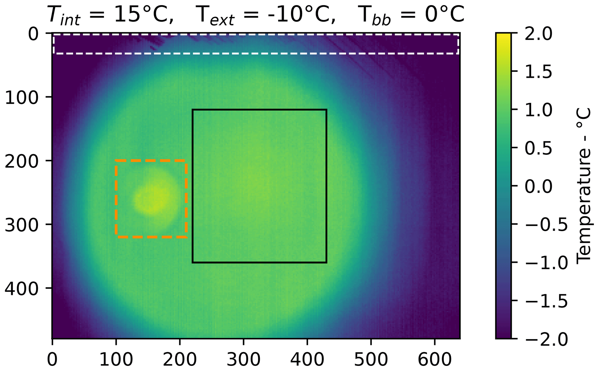
Figure 5 Image of the black-body target (0 °C) highlighting two areas with defective pixels. In the upper part, pixels were damaged by direct-sunlight exposure during the first year of deployment (white rectangle). On the left, pixels were subject to a warm error of unknown cause (orange rectangle). The area used for calibration is shown on the right (black rectangle).

4.3.2 Dependence on T_int−T_set

The difference between the average of the temperature measured for a specific internal and target temperature combination T_meas and the corresponding black-body temperature T_bb is represented in Fig. 7a and b for a set internal temperature T_set of 15 and 22 °C, respectively. The raw measurement and the black-body temperature corrected for observation through the window T_bb-win should be equal if the camera is perfectly calibrated. This is not the case; instead, we found that the difference between these two temperatures was proportional to the difference between the TEM's temperature setting T_set and the real internal temperature of the camera T_int (see Fig. 7c). Through a linear regression, the following relation was found:

$$\begin{array}{}\text{(4)}& T_{\mathrm{meas}}-T_{\text{bb-win}}=\mathrm{1.92}\cdot (T_{\mathrm{int}}-T_{\mathrm{set}})-\mathrm{1.33}.\end{array}$$

5 Processing

The processing of the TIR images consists of three main steps. First, the radiometric processing improves the quality of the measurements by correcting the instrumental issues described in Sect. 4. Second, images with poor or null visibility of the surface were deleted from the dataset. Third, during the geometric processing, image distortions were corrected, slight movements of the camera observed throughout the season were compensated for, and the images were orthorectified, i.e., projected onto a digital elevation model (DEM). The whole processing workflow is summarized in Fig. 6. Our method does not include corrections for non-instrumental effects such as emissivity and atmospheric contributions. We therefore consider these effects to be included in our error estimations.

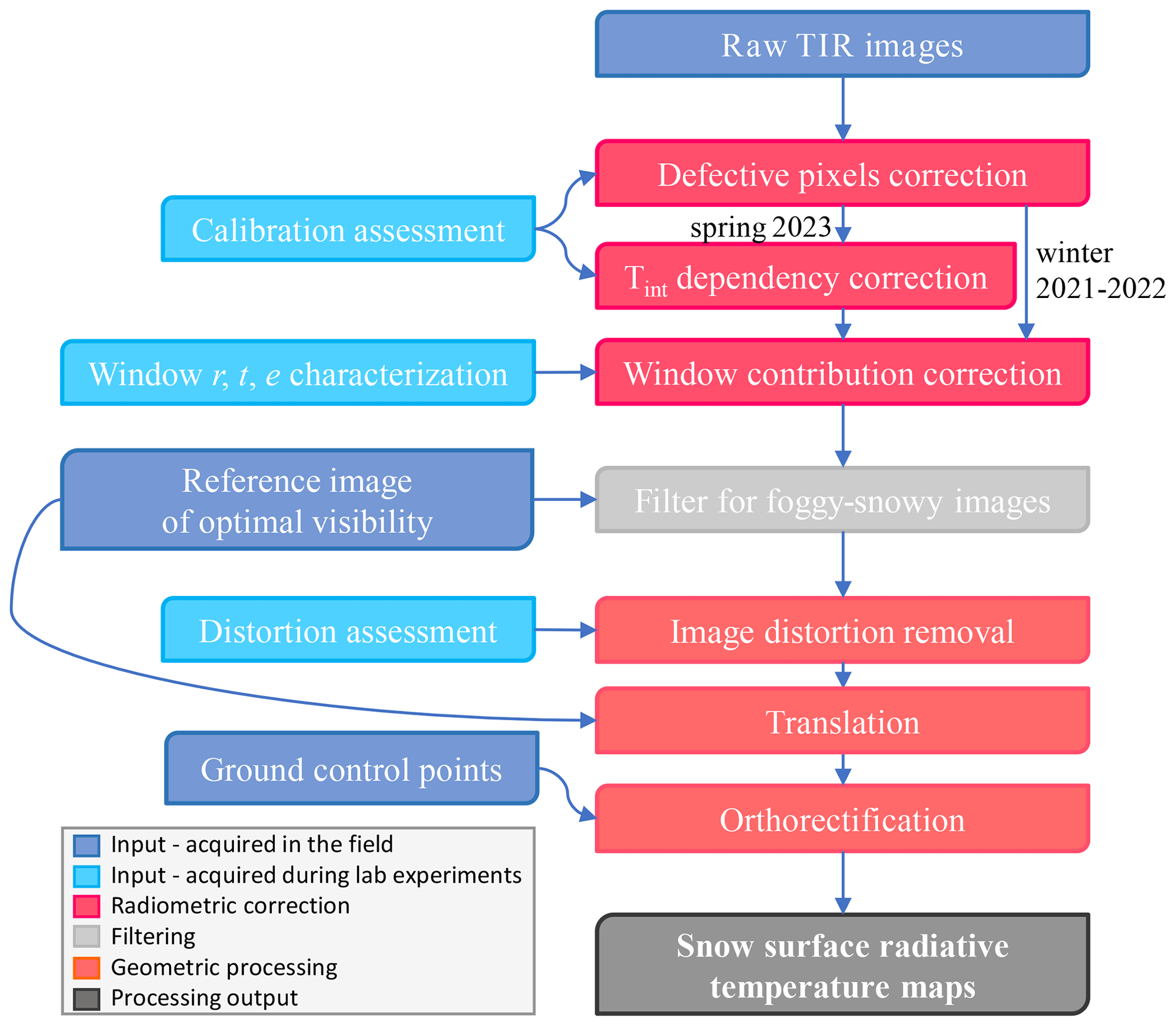
Figure 6 Workflow of the processing of raw TIR images to radiometrically corrected and orthorectified surface radiative-temperature maps.

5.1 Radiometric processing

The radiometric processing was performed in three steps. First, the warm error described in Sect. 4.3.1 was corrected. As the bias is considered to be constant over time, the average image of the warm error acquired during the TIR camera's characterization was subtracted from every image. Second, according to Eq. (4), the bias due to the T_int−T_set dependency was corrected for as follows:

$$\begin{array}{}\text{(5)}& T_{\text{meas\_corr}}=T_{\mathrm{meas}}-\mathrm{1.92}\cdot (T_{\mathrm{int}}-T_{\mathrm{set}})+\mathrm{1.33}.\end{array}$$

Third, the effect of the camera's window was corrected for:

$$\begin{array}{}\text{(6)}& \begin{array}{rl}& T_{\text{meas\_rad\_corr}}=\\ & {\left({\displaystyle \frac{\begin{array}{c}(T_{\text{meas\_corr}}+\mathrm{273.15}{)}^{\mathrm{4}}-r\cdot (T_{\mathrm{int}}+\mathrm{273.15}{)}^{\mathrm{4}}\\ -e\cdot (T_{\mathrm{win}}+\mathrm{273.15}{)}^{\mathrm{4}}\end{array}}{t}}\right)}^{\mathrm{0.25}}-\mathrm{273.15},\end{array}\end{array}$$

where T_win is taken as the average of T_int and T_ext. T_ext is measured at the AWS-South station, the closest to the camera. If that was not available, T_ext was taken from the automatic weather station FluxAlp (45.0413° N, 6.4106° E; Laurent et al., 2012) located on the east side of the Col du Lautaret, about 1 km from our site. The differences between the corrected measurements and the black-body temperatures are shown in Fig. 7d for an internal temperature of 15 °C and in Fig. 7e for an internal temperature of 22 °C. The residual errors span between −0.57 and +0.38 K and are distributed around 0 °C with a standard deviation of 0.22 K.

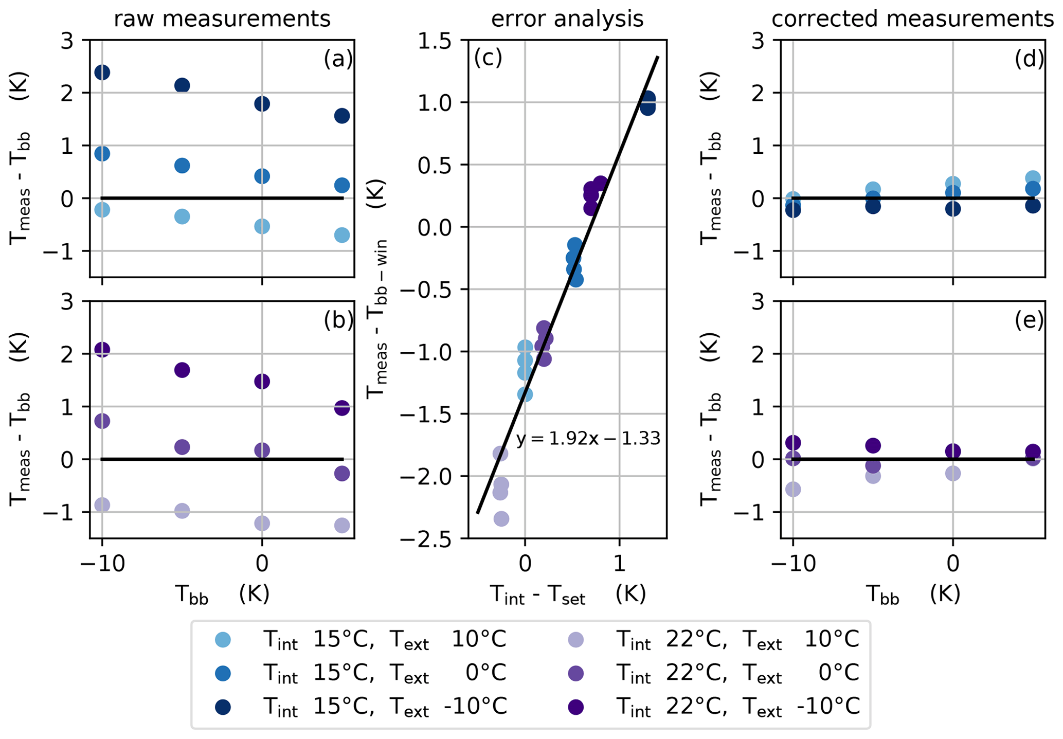
Figure 7 Difference between the average measured temperature T_meas and the actual black-body temperatures T_bb as a function of black-body temperature for internal temperatures T_int of 15 °C (a) and 22 °C (b). The difference between the raw measurement and the black-body temperature corrected for observation through the window T_bb-win as a function of the difference between the thermoelectric module setting T_set and the real internal temperature of the camera T_int (c). The differences between the corrected measurements and the black-body temperatures for an internal temperature of 15 °C (d) and 22 °C (e).

5.2 Cloud filtering

Transiting clouds and snowfall reduce the visibility of the surface from the TIR camera. To detect the presence of clouds, we relied on the detection of different objects that are clearly recognizable during days with optimal visibility. With this aim, the MatchTemplate function of the OpenCV Python library identifies the position of a given feature (i.e., a small reference image) in a complete TIR camera image as the location where the two overlapping images correlate most. The chosen reference image was taken at solar noon on one sunny day per year (5 March 2022 at 13:00 UTC+1 and 5 March 2023 at 13:00 UTC+1). The only snow-free features in the camera's FOV are the road and the vegetation. Both are warmer than the surrounding snow-covered soil.

Cloud filtering was performed in two steps. First, for every image, a 356 × 200 cropped image including a portion of the road was extracted (orange rectangle in Fig. 8). MatchTemplate computed the position of the cropped image in the reference image. If the returned position had an absolute error of ≥5 pixels for any of the x or y dimensions, the image was considered cloudy and rejected. If the returned position was correct up to an absolute error of <5 pixels for both dimensions, the road was considered recognized. The small detected displacements (0–4 pixels) of the evaluated image with respect to the reference image were considered as plausible since the camera moved slightly throughout the season. Second, two smaller features (trees) on the left and right sides of the image were cropped from both the reference and the evaluated image (white rectangles in Fig. 8). The Pearson correlations with respect to the reference were computed with MatchTemplate. If any of the two correlations was ≤0.25, the features were considered non-recognized and the whole image was considered cloudy. It was therefore rejected. Otherwise, the image was considered to definitely have sufficient visibility.

This method was tested against a set of ≈1000 manually chosen TIR images with good visibility on snow-covered terrain and ≈1000 images with conditions ranging from mist to thick fog. Among the days with a clear sky, only one image was discarded, which means a 0.1 % false-positive error. Of the images with poor visibility, 19 were retained, indicating that 1.9 % were false negatives. Despite this encouraging performance, the method proved to be inefficient at the beginning and at the end of the winter season, as the presence of large bare-ground patches altered the surface temperature patterns, which then no longer correlated with the snow-covered ground in the reference image. Thus, the classification was performed visually for the images acquired before 25 November 2021 and after 14 April 2022 for winter 2021–2022 and after 19 April 2023 for spring 2023.

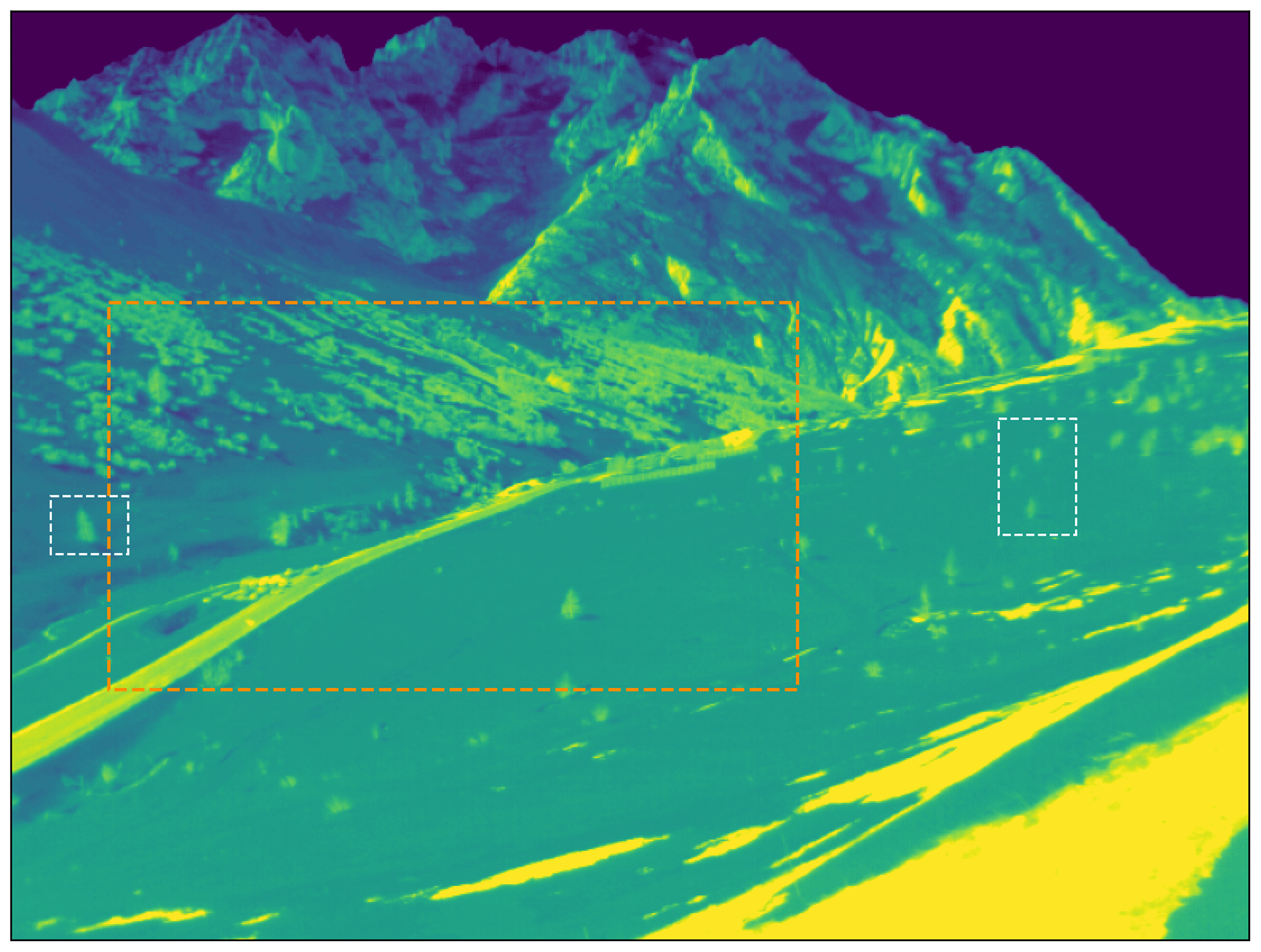
Figure 8 Areas of the image used to evaluate the overall visibility of the picture in relation to detecting displacement (orange rectangle) and evaluating the visibility of small features (two vegetation features indicated by white rectangles).

5.3 Geometric processing

Geometric processing aimed at obtaining accurate orthorectified maps of the snow surface temperature from radiometrically corrected and cloud-filtered TIR camera acquisitions. It was performed in three steps. First, image distortions were removed using the undistort function of the OpenCV Python library and the distortion parameters obtained during the TIR camera characterization. Second, the images were translated in order to compensate for the slight movements (of up to 4 pixels) of the TIR camera observed throughout the two seasons. The displacement was computed with the MatchTemplate function of the OpenCV Python library (see Sect. 5.2). The images were translated by the median displacement on the day of acquisition using the warpAffine function of OpenCV.

The orthorectification, which is the projection of the camera images onto a digital elevation model (DEM), was finally performed using the Ames Stereo Pipeline from NASA (ASP; Beyer et al., 2018) in two steps. First, the camera position was computed using the camera's focal length, the DEM, and GCPs. For this step, a 50 cm resolution DEM acquired by lidar on bare soil was used. Before the orthoprojection, 0.75 m was added to the DEM height to simulate the average snow cover height for the season. The coordinates (XY) of the GCPs in the TIR camera reference were extracted from the images after the translation. The camera position, which integrates the camera model, was obtained with the cam_gen function of ASP. Second, the mapproject command was used to project the images onto the DEM using the refined camera model. The output is a map of the surface temperature in geotiff format (464 × 506 pixels, 2 m resolution, single band, float32 data type, LZW compression), which is practical for importing into most geographic information software.

6 Results

The number of acquired TIR images of the Col du Lautaret site is over 103 000 for winter 2021–2022 and over 61 000 for spring 2023. The durations of the measurement periods are described in Fig. 9. Interruptions to the TIR camera measurements during winter 2021–2022 were due to electricity outages at the site, while missing TIR radiometer measurements during this period were due to battery problems that were solved during the spring. The missing measurements at the beginning of spring 2023 were due to camera overheating episodes. Partial snow cover is indicated for periods when snow is not present yet or has already melted at AWS-North and AWS-South but the soil at the Col du Lautaret remains partially covered with snow.

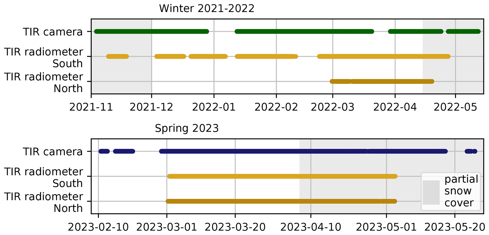
Figure 9 Periods of measurement of the surface radiative temperature of snow throughout winter 2021–2022 and spring 2023. Periods of partial snow cover, indicating no snow cover at AWS-South and AWS-North, are shaded.

The distributions of the raw and radiometrically corrected surface temperature measurements acquired at AWS-South and AWS-North during the two seasons are shown in Fig. 10. The values were extracted from the images before orthorectification and correspond to the average for four pixel squares corresponding to the radiometers' fields of view. The radiometric correction caused a decrease in the median measured temperature for all distributions. The decrease was more important for the winter 2021–2022 distributions than for the spring 2023 ones, with an average decrease of 1.62 K against 0.55 K. This difference is due to three factors. First, a stronger correction is performed for the window transmission during winter 2021–2022, which causes the measured temperature to decrease by 1.62 K during winter 2021–2022 but by only 1.12 K during spring 2023. This is caused by the higher average internal temperature of the TIR camera during the first campaign compared to spring 2023: 21.9 °C against 19.3 °C. Second, the correction for the dependence on T_int−T_set performed for measurements in spring 2023 caused an average increase of 0.66 K everywhere on the image. Finally, the measurements acquired at AWS-North during spring 2023 are the only ones affected by the warm-pixel area described in Sect. 4.3.1 among the presented distributions. The correction for the warm-pixel area causes a decrease of 0.17 K for all images.

The filtering of the images with unsatisfactory visibility resulted in 77 % of the images from winter 2021–2022 and 82 % of the images from spring 2023 being retained. An additional 16 600 measurements from the first season and 211 from the second one were excluded from the dataset as no measurement of the camera's internal temperature was available to use for radiometric processing. As a result, a total of 130 019 images (79 563 from 2021–2022 and 50 456 from 2023) went through geometric processing.

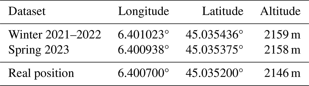
The triangulation of the GCPs on the DEM yielded similar camera positions for the two seasons, as illustrated in Table 2. The computed positions during the two seasons are higher than the real one by 13 and 12 m, respectively, and are 33 and 39 m NE of the real camera position. The median projection error of the GCPs was 4.3 m for winter 2021–2022 and 3.2 m for spring 2023, which was considered sufficient for the comparison with multi-decameter-resolution satellite images. The projection error for each GCP is listed in Tables A1 and A2 in Appendix A.

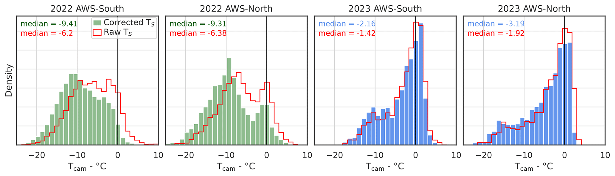
Figure 10 Distributions of the measured raw (red) and radiometrically corrected (green and blue) surface radiative temperatures of snow at AWS-South and AWS-North throughout winter 2021–2022 and spring 2023.

Table 2 Camera positions computed for the two datasets by the Ames Stereo Pipeline cam_gen function from the camera's focal length, the DEM, and the GCPs compared to the real camera position.

7 Validation

The validation of the 2-year dataset was performed using TIR radiometer data acquired at AWS-North and AWS-South in the TIR camera's FOV. The radiometers' specifications are described in Table 1, and their positions are shown in Figs. 1 and 2. The performance of the surface temperature measurement T_cam with respect to the ground truth T_rad is shown in Table 3. The error distributions are described using the median and the mean absolute error (MAE) in order to consider both the precision and the accuracy of the measurements. All distributions with a median or MAE ≤0.7 K (marked in bold) correspond to measurements acquired during spring 2023. Indeed, the lowest surface temperatures ($\le -\mathrm{1}$ °C) measured during the second season by the TIR camera have slightly negative to positive median biases, between −0.02 and +0.49 K, with respect to the TIR radiometer measurement. The MAEs meet the <0.7 K target except for the temperatures −5 °C $\le T_{\mathrm{cam}}\le -\mathrm{1}$ °C measured at AWS-South and the temperatures $\le -\mathrm{5}$ °C measured at AWS-North, which are slightly above (0.71 and 0.83 K, respectively). In particular, the larger MAE at AWS-North may be due to additional noise induced by the warm defective pixels that affect the area. The highest measured snow temperatures ($>-\mathrm{1}$ °C) during 2023 have the highest median differences with respect to T_rad, +1.17 K at AWS-South and +0.61 K at AWS-North. Indeed, during spring 2023, the measured surface radiative temperature measured by the TIR camera over melting snow is found to be higher than freezing point (0 °C) by several degrees, as shown in Fig. 11 (red circle). The cause of this temperature overshoot is unknown. The median and the MAE obtained if only temperatures $<-$1 °C are considered (0.22 and 0.68 K, respectively) are therefore much lower compared to those obtained for the whole distribution (0.48 and 0.82 K, respectively). The errors of the measured surface temperatures from winter 2021–2022 are always negative and range between −0.74 K and −1.95 K, with a median error of −1.05 K and an MAE of 1.28 K. None of the medians or MAEs for the first season meet the 0.7 K target. Some overshoots of the surface radiative temperature at 0 °C are also observed during winter 2021–2022. However, they are less visible in Fig. 11 because of the cold bias of the overall distribution and the reduced precision of the IR120 radiometers. Also illustrated in Fig. 11 are the linear regressions of the two distributions (orange lines) and the computed slopes, intercepts, fit R² values, and RMSEs (m, b, R², and σ_y, respectively). The regressions confidently fit both distributions, as shown by the elevated R² values of −0.96 for winter 2021–2022 and 0.97 for spring 2023. The first has an intercept $b=-\mathrm{1.81}$ °C, with the error decreasing with the temperature, as the slope m=0.91. The second, on the other hand, has an intercept $b=+\mathrm{0.52}$ °C, and the bias is fairly constant, as m=1.02.

Table 3 Distributions and statistics of the difference between the surface temperature measured by the camera T_cam and that measured by the radiometers T_rad. Distributions meeting the target for the median and MAE (≤0.7 K) are marked in bold.

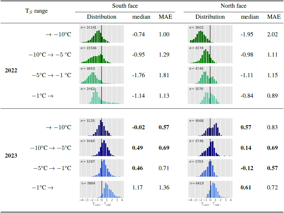
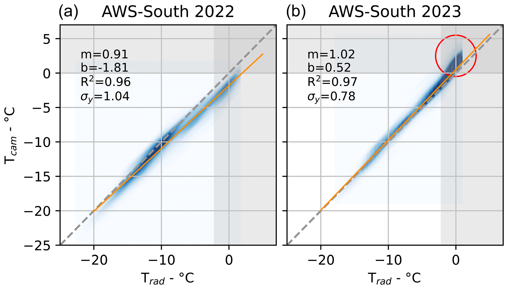
Figure 11 Density distributions of the snow surface temperatures measured at AWS-South by the camera as a function of those measured by the radiometer during winter 2021–2022 (a) and spring 2023 (b). High measurements of surface temperature measured during spring 2023 over melting snow are indicated by a red circle. Also shown are the identity line (dotted gray line) and the linear regression of the distribution (orange line).

8 Discussion

Surface radiative-temperature maps of the snow cover were acquired at the Col du Lautaret over winter 2021–2022 and spring 2023 with an uncooled TIR camera. The maps were continuously validated against surface radiative-temperature measurements performed by two high-precision TIR radiometers in the camera's field of view. This dataset also included measurements of the incoming longwave radiation, air temperature, and humidity, the wind speed measured on-site, the TIR radiometer temperature measurements, the TIR camera internal-temperature time series, and RGB images of the site.

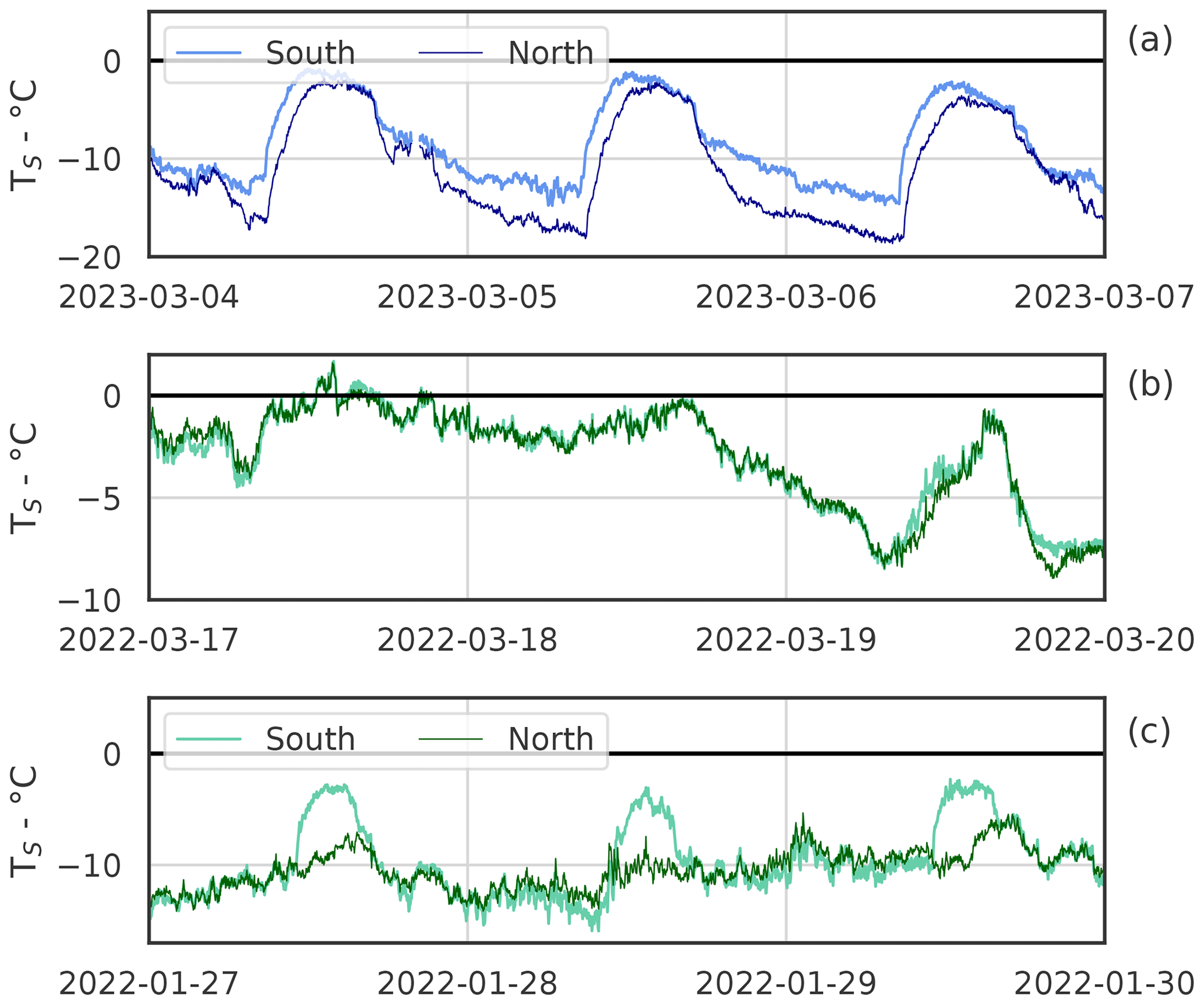
Figure 12 Three examples of the surface temperature time series measured by the TIR camera at AWS-South and AWS-North during a sunny spring period (a), a cloudy period (b), and a sunny winter period (c).

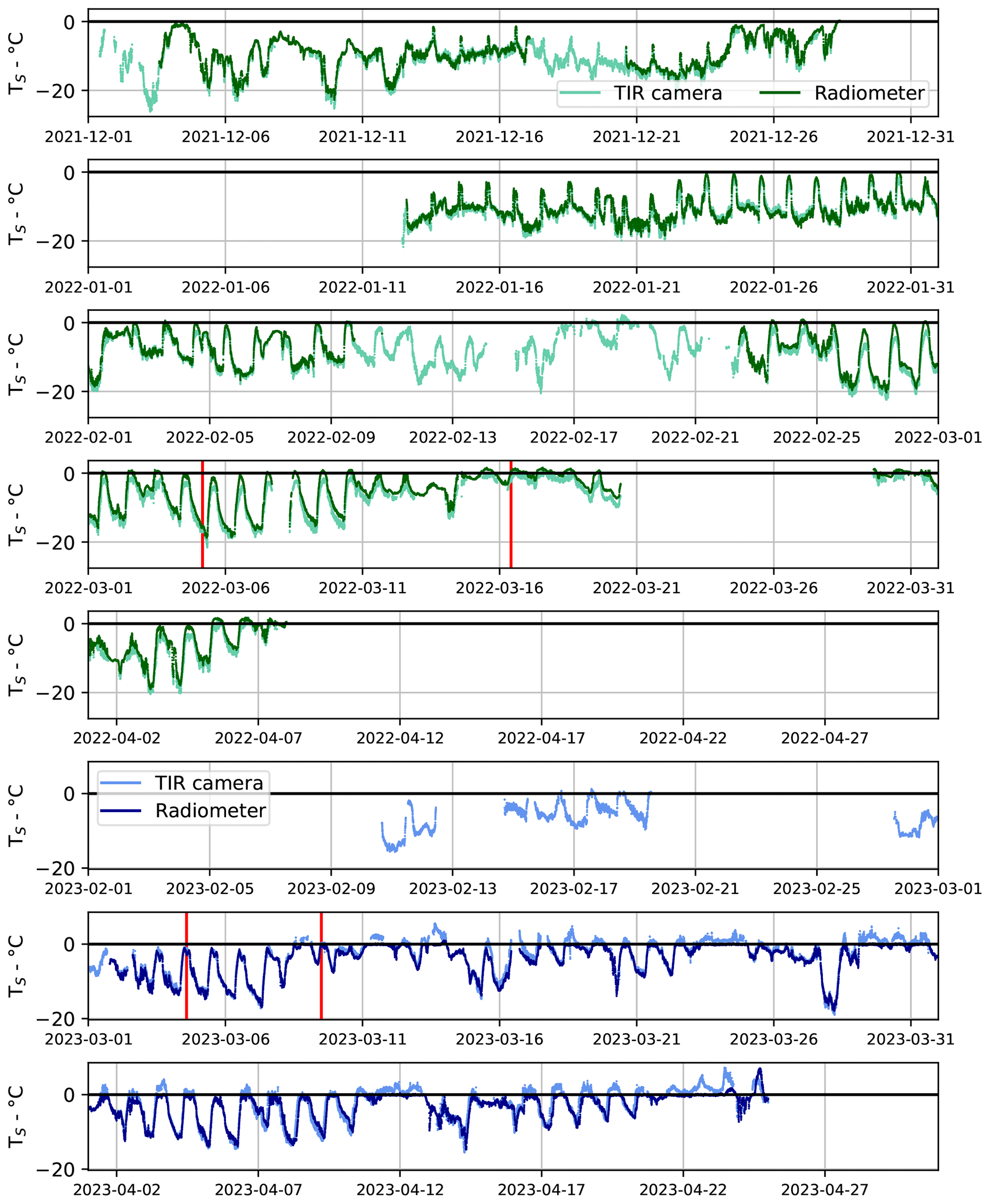
Figure 13 Full time series of the snow surface temperatures measured by the TIR camera and by the CT15.85 radiometer at AWS-South over the two seasons (winter 2021–2022 in green and spring 2023 in blue). The red lines correspond to the images in Fig. 14.

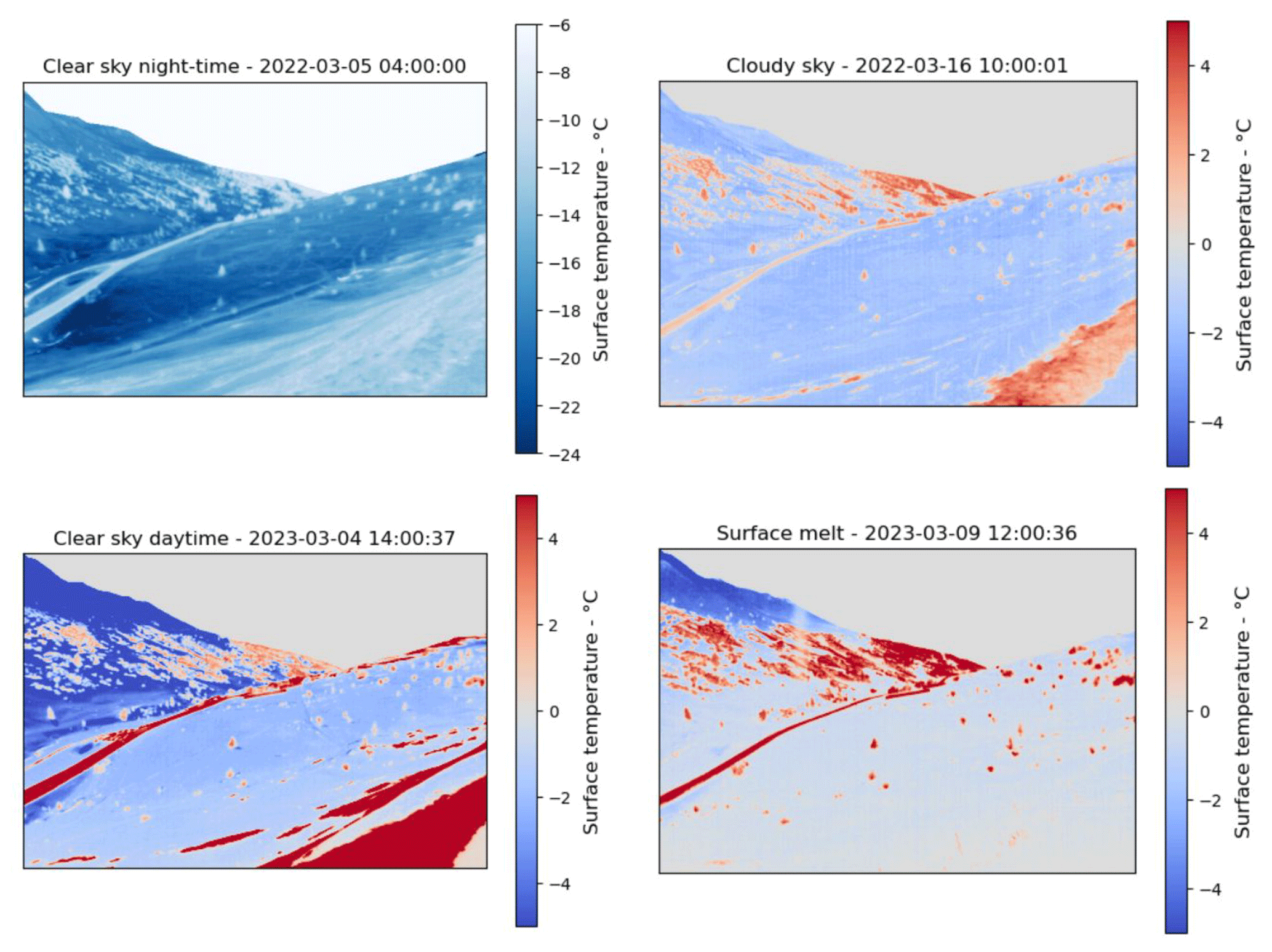
Figure 14 Four measurements of the snow surface temperature acquired using a TIR camera under different atmospheric conditions.

The processed measurements acquired during winter 2021–2022 exhibit a median error of −1.05 K and an MAE of 1.28 K, both of which are above the specified accuracy target of 0.7 K. The lower accuracy is clearly attributable to the inherent instability of the internal temperature of the thermal-infrared (TIR) camera throughout the season. The camera operated in its commercial configuration, resulting in a broad range of internal temperatures (7 to 39 °C) whose impact is not correctly compensated for by the internal FFC. Due to the absence of an internal-temperature reference, we are not able to retroactively apply the corrective measure for the variations in the internal temperature applied for spring 2023 to the 2022 dataset. Nevertheless, the 2022 dataset remains useful, as our measurements, with an accuracy of 1.28 K, perform better than the 1.5 K (1σ) target for the level 2A LST product of TRISHNA. To facilitate further investigation, the processed maps can be adjusted for the surface temperatures to match the ground truth (the average TIR radiometer measurement recorded at AWS-North and AWS-South) when available. The accuracy of the adjusted measurements is expected to be better.

During the second season, the instrumental setup was modified to limit the variations of the internal temperature of the camera, resulting in a clear improvement in measurement quality. With the internal camera temperature constrained, the observations exhibited improved precision and accuracy with respect to the 2021–2022 winter season, achieving the targeted errors. Overall, the median TIR camera measurement error relative to the ground truth (TIR radiometers, T_cam−T_rad) was reduced by a significant 54 % with respect to the previous season, going from −1.05 to +0.48 K. More impressively, the median error considering only measurements performed on cold snow ($T_{\mathrm{cam}}<-\mathrm{1}$ °C) was as low as +0.22 K, overcoming the absolute-temperature issues encountered by numerous previous studies (Aubry-Wake et al., 2015; Kraaijenbrink et al., 2018; Pestana et al., 2019). The MAE was equal to 0.82 K for the whole season and 0.68 K when considering measured temperatures of $<-\mathrm{1}$ °C only. We tested the possibility that the higher error for melting snow might be due to a thin layer of warmer water above the snow grains. Still, assuming a thermal conductivity of water (k) of 0.6 and a water film thickness of 0.5 mm, 1200 W m⁻² of absorbed energy would be needed to sustain a 1 K difference between the top layer and the bottom snow layer at 0 °C, which is not plausible. Therefore, the physical cause of this error is unidentified and remains to be investigated. However, this error is always a warm bias and is therefore easy to identify and correct, as the snow temperature is physically limited to 0 °C when the pixels are fully covered by snow. Such a correction can be applied to periods when snow on the ground at the two AWSs is clearly recognizable on the images acquired by the RGB camera throughout the season.

Another limitation of the current dataset concerns the emissivity. We assume that snow is a perfect black body and do not attempt to apply an emissivity model due to the lack of consensus on the topic. However, the emissivity of snow is known to be slightly lower than 1 (Hori et al., 2014) and to decrease with the observation angle, especially for angles over 45° in the 12–14 µm TIR window (Dozier and Warren, 1982; Hori et al., 2006). We assume that this error is included in the global error assessed by the comparison with the ground truth. To facilitate further analysis by data users, a map of the observation angles of the area, computed as in Castel et al. (2001), is included in the dataset. Moreover, downwelling longwave measurements performed at the Col du Lautaret site are supplied (FluxAlp measurements for winter 2021–2022 and AWS-North and AWS-South measurements for spring 2023). With these measurements, the surface radiative temperatures can be adjusted to accommodate for emissivity values <1.

Similarly, the measured temperature depends on the radiative contribution of the air between the sensor and the target, which was not corrected for and is therefore considered part of the error measured in the comparison with the ground truth at the two AWSs. Still, as this error increases with the viewing distance, a distance-to-camera map is included in the dataset, and this can be used with temperature and humidity measurements from the AWSs to correct for the atmospheric contribution.

Dataset users should take into account that the camera FOV contains not only snow but also rocks, trees, a road, and wood fences. Moreover, during the orthorectification process, the DEM projects some vertical features such as tall trees or wood fences long distances behind their actual positions because of the oblique angle at which the camera is installed. This is always the case behind the snow fences in the central part of the image and can happen when cars are driving on the road in the camera's FOV (Fig. 2).

Overall, obtaining accurate measurements of the surface temperature with a TIR camera is challenging and time consuming, as it requires a large number of complementary measurements and laboratory experiments (see Fig. 6). The radiometric correction compensates for a combination of warm bias (from the window contribution and warm pixels) and cold bias (from the T_int−T_set dependence). Thus, for accurate measurements, it is fundamental to compute all biases correctly in order to avoid an apparent accuracy due to compensation between positive and negative errors. As such, we recommend performing a comprehensive characterization of the camera and testing the calibration frequently, at least once per winter season.

All this considered, we conclude that the efforts put in to stabilize the internal temperature of the Optris Pi640 TIR camera led to accurate measurements of snow surface radiative temperature, with an overall accuracy below 0.7 K achieved, which is comparable to the radiometric accuracy expected for the TIR instrument of the TRISHNA satellite and the high-resolution TIR sensors that will follow.

The example time series shown in Fig. 12 illustrate the potential of the dataset to characterize the drivers of snow surface temperature. Two time series, (a) and (b), were acquired during sunny, clear-sky periods. Time series (a) was acquired in spring and shows similar daily surface temperature cycles for AWS-South and AWS-North. Indeed, in spring, the two areas have comparable exposures to sunlight, which drives the surface temperature, causing the cosine shape of the profile in the middle of the day. Likewise, in time series (b), acquired during a cloudy period, the temperature profiles of the two sites are very similar, showing that the energy budget of the surface is driven by terms that are barely affected by the topography. In time series (c), however, the temperatures differ significantly. The cosine shape is significantly smaller at AWS-South than in time series (a) and is absent at AWS-North, as AWS-South receives some sun while AWS-North remains in the shadow during winter. This illustrates how different processes can drive the surface temperatures at these two sites separated by a distance as small as 300 m (i.e., less than the pixel size of MODIS, VIIRS, or Sentinel 3 SLSTR) and at similar altitudes. The full time series are shown in Fig. 13. Finally, the images in Fig. 14, acquired under different atmospheric conditions, show the variability of the patterns of the surface temperature of snow caught by the TIR camera. Besides these examples, the dataset provides numerous other situations that deserve further exploration.

9 Data availability

Snow surface radiative-temperature maps and ancillary data can be found at https://doi.org/10.57932/8ed8f0b2-e6ae-4d64-97e5-1ae23e8b97b1 (Arioli et al., 2024a) and https://doi.org/10.57932/1e9ff61f-1f06-48ae-92d9-6e1f7df8ad8c (Arioli et al., 2024b). The data are partitioned into two datasets, one for winter 2021–2022 and the other for spring 2023. Both contain maps of the surface temperature of snow acquired at the Col du Lautaret every 2 min, RGB images of the scene acquired every 10 min during the operation of the TIR camera, time series of the surface temperature acquired every 30 s at AWS-North and AWS-South, and the TIR camera’s internal temperature acquired every 2 s. The dataset from spring 2023 also includes time series of measurements acquired every 30 s of the incoming longwave radiation, air temperature, and air humidity at both AWS-North and AWS-South and of the wind speed at AWS-South only. Each dataset contains zip files corresponding to the week of the year of acquisition (starting each Monday). For example, 2023_w06.zip refers to week 6 of the year 2023. Every .zip file contains folders with the data separated by day. Within each day folder, the maps_Ts folder contains single-band surface temperature maps in the EPSG:32632 projection in geotiff format with LZW compression. These are 464 × 506 pixels wide at 2 m resolution and contain float32 data. The RGB folder contains the visible images of the scene. The file Camera_Tint.csv contains the time series of the internal temperature of the TIR camera. The files AWS_north.csv and AWS_south.csv contain time series of data measured at AWS-North and AWS-South, respectively. More details are given in the README.md file in each dataset.

10 Conclusions and perspectives

This study presents a dataset of 130 019 georeferenced geotiff images of the surface radiative temperature acquired at the Col du Lautaret in the French Alps. Thermal-infrared images were acquired with an Optris PI640 uncooled TIR camera during winter 2021–2022 and spring 2023. The resulting surface radiative-temperature maps from the first season have a radiometric accuracy of 1.28 K (mean absolute error) after processing. The TIR camera was run with an improved setup during spring 2023, reaching a radiometric accuracy of 0.67 K (mean absolute error) for surface temperatures below −1 °C and 1.17 K for melting snow. The results show how the internal-temperature stabilization of the TIR camera integrated into the spring 2023 setup strongly benefited both the precision and the accuracy of the measurements, overcoming the original issues. This study also confirms that performing accurate measurements of the surface temperature of snow with TIR cameras is challenging and requires camera adaptation, additional field measurements, time-consuming laboratory experiments, and – in any case, despite the level of effort – high-precision TIR radiometers used as ground truth to achieve the absolute accuracy target. Still, the obtained measurement accuracy is comparable to those of multiple spaceborne TIR sensors and better than most derived LST products. This dataset is, to our knowledge, unique and should benefit the investigation of topographic effects on remote sensing and the link between snow emissivity, snow grain characteristics, and observational angles. Also, the measurement technique described in this study represents a potential advance in the calibration–validation of satellite-derived surface temperature products in regions characterized by snow cover and a complex topography, providing an evaluation tool for thermal-infrared products from Landsat or ECOSTRESS. The know-how gained from this study will be instructive for the calibration–validation of upcoming high-resolution thermal-infrared missions, starting with TRISHNA at the end of 2026. Finally, considering the increasing use of uncrewed aerial vehicle (UAV) measurements employing TIR cameras over cryospheric surfaces (Gök et al., 2023; Rossini et al., 2023; Wigmore and Molotch, 2023), the present configuration for a stationary camera can serve as a foundational framework for future UAV applications. In fact, the first trials of UAV measurements of the snow surface temperature with a TIR camera with a similar improved setup are underway.

Appendix A

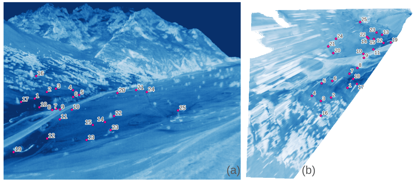
Tables A1 and A2 show the positions of the ground control points (GCPs) used for the orthorectification of the TIR imagery. There are 21 GCPs for winter 2021–2022 and 25 for spring 2023. Their positions are supplied both in world and camera coordinates, and the error projection for each GCP is given. Figures A1 and A2 show the spatial distribution of the GCPs for winter 2021–2022 and for spring 2023, respectively. The distribution is shown in both camera coordinates and longitude–latitude coordinates (EPSG:4326).

Table A1 List of the GCPs used for the orthorectification of the thermal-infrared images acquired during winter 2021–2022. The positions of the GCPs in both camera coordinates (X, Y) and world coordinates (longitude and latitude; EPSG:4326) are supplied. The last column indicates the error projection computed by the Ames Stereo Pipeline during the triangulation of the GCPs.

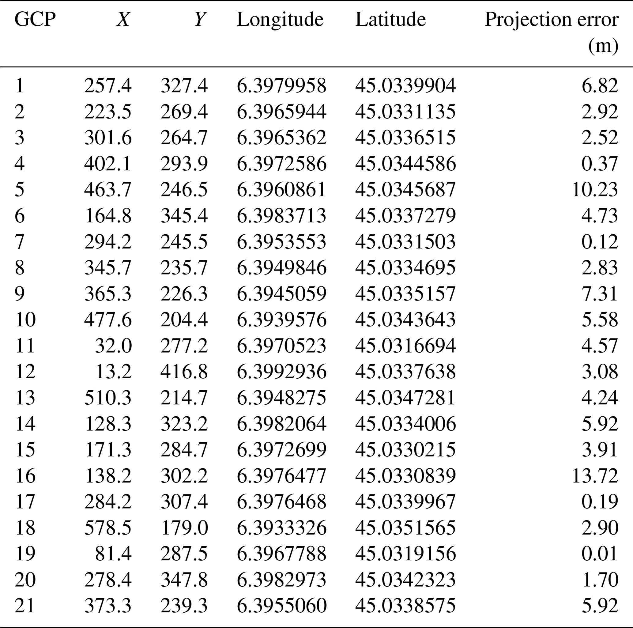
Table A2 List of the GCPs used for the orthorectification of the thermal-infrared images acquired during spring 2023. The positions of the GCPs in both camera coordinates (X, Y) and world coordinates (longitude and latitude; EPSG:4326) are supplied. The last column indicates the error projection computed by the Ames Stereo Pipeline during the triangulation of the GCPs.

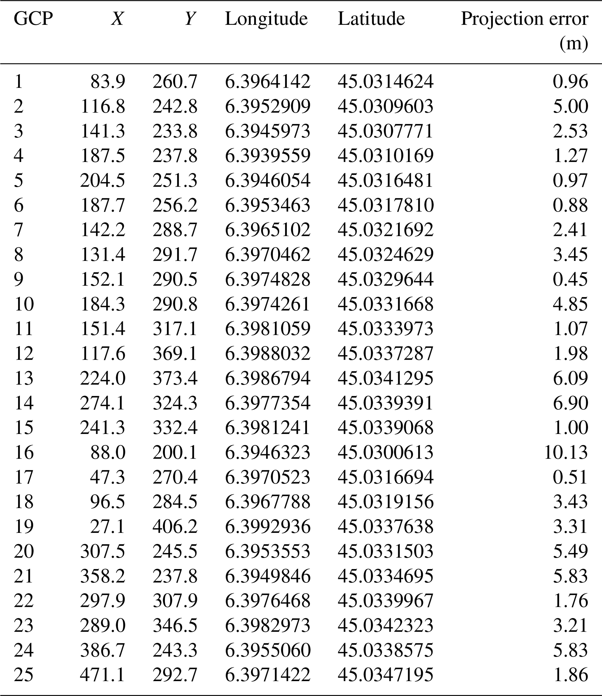
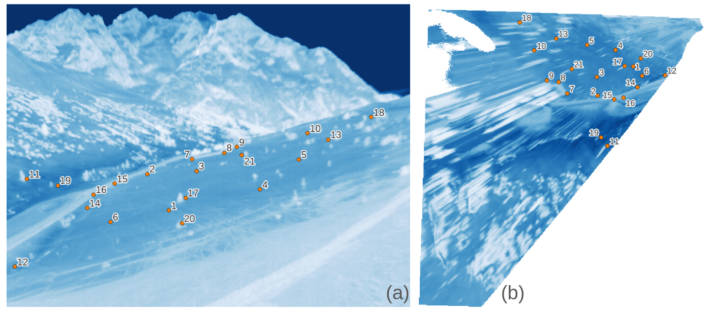
Figure A1 Spatial distribution of the GCPs listed in Table A1 in camera coordinates (a) and world coordinates (longitude and latitude; b).

Figure A2 Spatial distribution of the GCPs listed in Table A2 in camera coordinates (a) and world coordinates (longitude and latitude; b).