MAP-IO: an atmospheric and marine observatory program on board Marion Dufresne over the Southern Ocean

This article is devoted to the presentation of the MAP-IO observation program. This program, launched in early 2021, has enabled the observation of nearly 700 d of measurements over the Indian and Southern Ocean with the equipment of 17 meteorological and oceanographic scientific instruments on board the ship Marion Dufresne. Several observational techniques have been developed to respond to the difficulties of observations on board the ship, in particular for passive remote sensing data, as well as for quasi-autonomous data acquisition and transfer. The first measurements made it possible to draw up unprecedented climatological data of the Southern Ocean regarding the size distribution and optical thickness of aerosols, the concentration of trace gases and greenhouse gases, UV, and integrated water vapor. High-resolution observations of phytoplankton in surface waters have also shown a great variability in latitude in terms of abundance and community structure (diversity). The operational success of this program and these unique scientific results together establish a proof of concept and underline the need to transform this program into a permanent observatory. The multi-year rotations over the Indian Ocean will enable us to assess the trends and seasonal variability of phytoplankton, greenhouse gases, ozone, and marine aerosols in a sensitive and poorly documented climatic region. Without being exhaustive, MAP-IO should make it possible to better understand and assess the biological carbon pump, to study the variability of gases and aerosols in a region that is remote in relation to the main anthropogenic sources, and to monitor the transport of stratospheric ozone by the Brewer–Dobson circulation. The meteorological MAP-IO data set is publicly available at https://www.aeris-data.fr/catalogue-map-io/ (last access: 26 August 2024) (atmospheric data) and at https://doi.org/10.17882/89505 (Thyssen et al., 2022a) (phytoplankton data).

1 Introduction

Due to its remoteness, the Southern Ocean (south of 35° S) is one of the least studied oceans in the world. Recently, Skinner et al. (2020) showed the important role of Southern Ocean convection as a potential amplifier of Antarctic warming and atmospheric CO₂ rise. The Circumpolar Current is the most powerful (130 ${\mathrm{Mm}}^{-\mathrm{3}}{\mathrm{s}}^{-\mathrm{1}}$) and has the strongest surface currents (0.9 to 3.7 km h⁻¹) in the world. This strong oceanic current, associated with strong quasi-permanent surface winds of the meridional overturning circulation, creates the conditions of important ocean–atmosphere exchanges that contribute significantly to the Earth's climate (e.g., Mayewski et al., 2009; Abernathey et al., 2011; Marshall and Speer, 2012; Nicholson et al., 2022). For example, Gruber et al. (2019) estimated that 40 % to 50 % of the global absorption of atmospheric CO₂ by the ocean occurs in the Southern Ocean. However, in the context of climate change, the evolution of the ocean CO₂ sink remains uncertain. This uncertainty is particularly strong in the Indian and Southern oceans due to the lack of atmospheric observations to better constrain inversions (Le Quéré et al., 2007; Landschützer et al., 2015; DeVries et al., 2017) and the lack of seasonal and intra-seasonal observations. The SOCAT (https://socat.info, last access: 8 November 2023) and GLODAP (http://www.glodap.info, last access: 8 November 2023; Lauvset et al., 2021) databases illustrate the crucial lack of data collection in this region in comparison with that carried out in the North Atlantic or in the equatorial Pacific.

From an atmospheric point of view, the lack of atmospheric observations over the Southern Ocean poses several problems, such as for numerical weather forecasts (data assimilation), for climate models (long-term observation), and for calibration and/or validation of spaceborne sensors. Recently, the World Meteorological Organization (WMO) has emphasized this need to address operational and scientific issues (Thurston et al., 2021). For example, the observation of atmospheric water vapor is crucial because of its key role in the weather and climate system. Its spatio-temporal evolution is at the origin of many meteorological phenomena, sometimes intense and poorly modeled by numerical weather forecasting models. In the longer term, its evolution is an indicator of climate change through its strong link with atmospheric temperature. The world's oceans produce nearly 86 % of atmospheric water vapor (Bengtsson, 2010) but are the areas where its observation is most patchy, being limited to surface or satellite observations (Smith et al., 2019). Within the troposphere, understanding the transport and the aging of aerosols over sea is an important challenge both for the climate budget and for the numerical weather forecast. The formation, the cloud condensation nuclei (CCN), and the ice-forming nuclei (IFN) properties of marine aerosols are still poorly understood, especially in areas where the production of organic matter by phytoplankton is important (Charlson et al., 1987; Quinn and Bates, 2011; Sellegri et al., 2021). The emission processes of marine aerosols and sea spray are also poorly known and parameterized in numerical models under strong wind and heavy swell conditions (Canepa and Builtjes, 2017; Pianezze et al., 2018; Sauvage et al., 2021). The challenges relate, in particular, to our ability to better understand and predict storms, deep convection, and tropical cyclones (Ramanathan et al., 2001; Hoarau et al., 2018; Sroka and Emanuel, 2021). Moreover, the southern Indian Ocean, mainly loaded with sea salt aerosols, is also impacted by long-range transport pathways connecting South America, southern Africa, Australia, and Southeast Asia to this part of the world, leading to a low yet highly variable aerosol burden (Duflot et al., 2022, and references therein). Indeed, these source regions are exposed yearly to the Southern Hemisphere biomass burning (BB) season and show records of extreme wildfires (e.g., the 2020 Australian wildfires). These BB events emit large quantities of gases and particles into the atmosphere (Andreae and Merlet, 2001), including carbon monoxide (CO) and fine smoke particles (black carbon (BC) and organic matter). Chemistry in the fire plumes involving CO may lead to the formation of tropospheric and stratospheric ozone (Crutzen and Andreae, 1990), which may exert a significant climate forcing in downwind regions. Emitted BC particles are highly absorbing by nature and contribute to reducing the cooling produced by scattering-dominated carbonaceous aerosols (Jeong and Wang, 2010). This effect is highly season-dependent and can extend to greater scales (from regional to global) when the particles are injected into the stratosphere. The penetration of smoke-related compounds into the stratosphere is thought to be more frequent in a warming world and depends on pyroconvection mechanisms (Fromm et al., 2000), as well as on the tropopause, which acts as a dynamical barrier. Therefore, the climatic impacts of such plumes should be assessed in this poorly documented part of the world. However, monitoring of atmospheric changes in the free troposphere and stratosphere over the Indian Ocean is sorely lacking, with only two NDACC stations (https://ndacc.larc.nasa.gov, last access: 26 August 2024) located on Réunion Island (21° S) and Kerguelen Island (49.3° S). The spatial distribution of key radiatively active trace gases, such as ozone in the stratosphere, is largely affected by the Brewer–Dobson circulation (BDC), characterizing three latitudinal regions from the Equator to the poles (Butchart, 2014): (i) the tropical stratosphere reservoir, (ii) the strong mixing mid-latitude surf zone, and (iii) the polar vortex. These regions are separated by a permanent subtropical dynamical barrier and a winter polar barrier. Chemistry–climate and climate models predict a strengthening of the BDC, especially within its shallow branch, due to the increase in greenhouse gases (Abalos et al., 2021). Observing ozone over a wide area of the Indian Ocean with repeatable trajectories will enable robust characterization in the different regions separated by these dynamic barriers.

From the point of view of marine microbial ecology, the Southern Ocean is depicted as the most productive ocean on Earth; with a clear boundary between the southwestern oligotrophic Indian Ocean, dominated by cyanobacteria; the Subantarctic Zone, dominated by haptophytes (<10 µm); and the south of the Polar Front, dominated by nano-eukaryotes (a polyphyletic group with cell size between 2–3 and 20 µm) and diatoms (Iida and Odate, 2014). The direct link between phytoplankton production and krill biomass sustaining the trophic conditions in the area makes phytoplankton a major group to study, especially in the currently expected conditions of climate change. A large part of the export of carbon in the area is controlled by the mixing pump (Nowicki et al., 2022), one of the elements most directly affected by the temperature increase. Contrasting scenarios are expected; indeed, an air temperature increase in the southern Indian Ocean is expected to amplify the oligotrophic conditions led by stratification and, reversely, intensify wind blowing due to the El Niño–Southern Oscillation (ENSO) variability (Wang et al., 2022). The latter would increase mixing, enhancing primary production by favoring the input of nutrients produced deeper by mineralization of the organic matter. Both scenarios will clearly influence the carbon biological uptake of CO₂ and the trophic status of the area. In Auger et al. (2022), the Southern Ocean below the southwestern Indian Ocean evidenced a small decrease in surface temperature, suggesting an increase in mixing, with a potential increase in production, but this does not account for the deep layers of global heating (Sallée, 2018). Little knowledge on the distribution of phytoplankton functional groups in the Southern Ocean and the southwestern Indian Ocean, as well as in the highly productive fronts, makes the estimation of the biological pump and the potential of energy transfer to the higher trophic levels difficult to forecast. The direct relation observed between phytoplankton functional group distributions and CCN (Sellegri et al., 2021) makes the investigation of both variables crucial for a holistic understanding of the effect of climate change in the study area.

The MAP-IO (Marion Dufresne Atmospheric Program – Indian Ocean) program aims to overcome the lack of observations in this region of the Earth, which is poorly documented compared to the other oceans, by equipping the Marion Dufresne vessel (https://taaf.fr/en/marion-dufresne-and-astrolabe, last access: 8 November 2023) with a set of in situ and remote sensing instruments for atmosphere and marine studies. This program has been labeled by the French Commission Nationale de la Flotte Hauturière (CNFH, https://www.flotteoceanographique.fr/en, last access: 8 November 2023) for the period 2021 to 2024. During this period, MAP-IO will operate as a scientific program for the acquisition and scientific enhancement of 4 years of data. This period will also serve as an operational prototype to study the feasibility of switching the program to a permanent observatory aimed at integrating the international infrastructure networks such as ACTRIS (https://www.actris.eu, last access: 8 November 2023) or ICOS (https://www.icos-cp.eu, last access: 8 November 2023). This article aims to present the MAP-IO program. It is organized as follows: the first part will present the objectives and the operating framework of the program. The second section will present the instrumental setup, while the third one will describe the information technology deployed for this purpose. The acquisition and archiving of data, as well as the website of the program, will also be presented in the third part. A preliminary presentation of the scientific results after 30 months of data collection will constitute the fourth part. The last section will be devoted to the conclusion and perspectives.

2 Framework and objectives

The Marion Dufresne is a large multipurpose vessel (120 m long and 4900 t). Under charter by the TAAF (https://taaf.fr/en, last access: 8 November 2023), this vessel is intended for the supply and transport of personnel across the southern lands and the scattered islands of the Mozambique Channel. It generally performs four annual rotations from Réunion Island (home port) to the islands of Crozet, Kerguelen, and Amsterdam (123 d per year). The rotation to the scattered islands is less frequent (once every 4 years or so) and is done around Madagascar through the Mozambique Channel. During the rest of the year (217 annual days on average), the ship is devoted to scientific research. It is then managed by the French oceanographic fleet (FOF, https://www.flotteoceanographique.fr/en, last access: 26 August 2024) and is operated under various sea campaigns whose scientific proposals are evaluated by the CNFH.

The MAP-IO program carries out atmospheric observations at the ocean–atmosphere interface and is integrated on the atmospheric column over the entire globe, with a particular interest in the study of the Indian and Southern oceans. The goal of the MAP-IO program is to study the feasibility of establishing a permanent marine observatory on board the Marion Dufresne. The program has three main objectives: (i) integration into international atmospheric and oceanic networks by providing high-quality data on a region devoid of permanent observations, (ii) validating and calibrating space sensors and numerical weather forecasting models, and (iii) monitoring global changes and interannual variability by continuous observation of the atmosphere and phytoplankton over the Indian and Southern oceans. MAP-IO takes advantage of the various scientific campaigns at sea planned by the FOF by exploring different poorly documented ocean areas and by increasing and completing the observation systems of the programs with additional measurements. The differentiation value of MAP-IO versus conventional scientific programs at sea is that it also relies on the regular rotations of the TAAF dedicated to visiting the French Austral islands by documenting the atmosphere and the ocean surface states over a wide variety of seas and latitude conditions. These multi-year observations of the Indian and Southern oceans make it possible to uniquely document the trends, the mechanisms of ocean–atmosphere exchanges, and the atmospheric composition on a seasonal and interannual basis. The large collection of the in situ data of MAP-IO under different latitudes and seasons, sea states, and meteorological conditions should provide important potentialities of machine learning uses. The potential near-real-time transmission of most MAP-IO observations is intended to fill an important data gap over the Southern Ocean in the assimilation or validation–calibration processes of numerical air quality or forecast models. Launched in the beginning of 2021, MAP-IO has already recorded nearly 700 measuring days at sea as of July 2023 (∼75 % of the time). In addition to the nine TAAF rotations on southern lands, the program's instruments have been previously utilized in 12 scientific campaigns dedicated to various fields such as volcanology, geology, geochemistry, sedimentology, oceanography, and marine biology.

3 Description of instruments and treatment methods

3.1 Instrument locations

The Marion Dufresne scientific vessel has embedded 17 scientific instruments on board, representing more than 25 atmospheric and marine biological parameters. Figure 1 illustrates the location of these instruments and computer servers on the ship. The optical measurements of cloudiness and UV radiation are located on the front mast of the ship at 20 m above sea level (a.s.l.). This forward position is a trade-off limiting the contamination of the measurements by the exhaust fumes of the ship. Under this mast is the dedicated computer acquisition room. The gas and aerosol inlets are located on deck I (20 m a.s.l.), oriented towards the front of the deck to reduce the possible contamination of the air sampled by the ship's activities. The in situ analyzers are located below the inlets. All the instruments and data acquisition computers are mounted on a shock-absorbing table in order to preserve the durability of the systems, particularly during strong swell conditions. This room is located next to the wheelhouse that facilitates the maintenance of instruments. Note that, for the quality of the atmospheric aerosol measurements, particular attention was paid to minimizing the distance (8 m) and the elbows of the air-conveying hose pipes. After testing several GNSS (Global Navigation Satellite System) antenna locations on the ship, the antenna has been positioned at the back of the vessel on deck J. This particular location was constrained to limit signal interference with the ship's instrumentation (radar, iridium beacon). Meteorological stations, the sun–sky–moon photometer, and the Mini-SAOZ (Système d'Analyse par Observation Zénithale) are located on the ship handle of the vessel at 25 m a.s.l., about 10 m in front of the funnel. An automated pulse shape recording and imaging flow cytometer (CytoBuoy, NL) is installed on a bench in a dry laboratory close to the thermosalinograph (Sea-Bird, SBE21), which allows it to be coupled with the ship's clean seawater circuit. The last area concerns the concentrator servers located in the information technology (IT) room (informatic room). These servers are connected to the IT system of the vessel. This connection allows us to be connected to the satellite internet network of the vessel and to get the ship location and some sea surface measurements, such as of sea surface temperature (SST), salinity, and sea waves and currents. All instruments and data acquisition methods are described below and are summarized in Table 1.

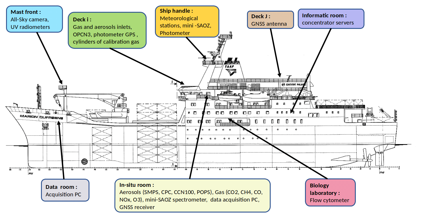
Figure 1 Location of the MAP-IO instruments and informatic servers on board the Marion Dufresne vessel.

3.2 Pulse-shape-recording flow cytometry

Automated flow cytometers for pulse shape recording and imaging, such as the Cytosense (Cytobuoy b.v.), have been used successfully on ships of opportunity, scientific vessels, and a buoy and in coastal observatories for several weeks without human action, collecting data on phytoplankton size classes at the single-cell level in an autonomous way (Thyssen et al., 2008, 2011, 2015; Marrec et al., 2018; Louchart et al., 2020). Phytoplankton abundance and functional groups are resolved on the basis of their size and pigment content when cells pass in front of a laser beam. The Cytosense automatically analyzes samples for phytoplankton counts in the size range of 0.6–800 µm in width and several millimeters in length. The seawater sample is funneled with a weight-calibrated sample pump into an injector, where it is surrounded by an isotonic sheath fluid, generating a laminar flow and forcing particles in a single-file fashion before entering the measurement cuvette, where it goes through a 120 mW 488 nm laser beam (Coherent^®). In doing so, a set of optical curves, called pulse shapes, are generated for each recorded particle. The pulse shapes of side-ward scatter (SWS, 488 nm) and fluorescence emissions were separated by a set of optical filters (orange fluorescence (FLO, 515–650 nm) and red fluorescence (FLR, 668–726 nm)) and were collected in photomultiplier tubes. The pulse shapes of forward scatter (FWS) were collected on left- and right-angled photodiodes and were used to validate the laser alignment. Samples are scheduled to be analyzed every 2 h from a stabilized 300 cm⁻³ sub-sampling chamber before the acquisition. The instrument and the acquisition protocol are described in Marrec et al. (2018). For the identification of phytoplankton groups, two protocols were successively run, one triggering on FLR of 5 mV for 5 min, targeting RedPicoProk and OraPicoProk, and a second one triggering on FLR of 20 mV for 10 min, targeting the RedPico, RedNano, OraNano, HsNano, RedMicro, and OraMicro phytoplankton groups (Thyssen et al., 2022b). Phytoplankton groups were manually classified using the CytoClus^® software by generating several two-dimensional cytograms and plotting descriptors of the four pulse shapes, such as the area under the curve of the pulse shape signals (total FWS). Group abundance and cell properties were processed by the software. The sizes of the different phytoplankton cells were estimated based on the relationship between silica bead real sizes (1.0, 2.01, 3.13, 5.02, and 7.27 µm non-functionalized silica microspheres, Bangs Laboratories, Inc.) and total FWS signal and were then converted into equivalent spherical diameter (ESD) and biovolume. A power-law relationship following the procedure in Marrec et al. (2018) allowed the conversion of the total FWS signal into cell size. The stability of the optical unit is routinely checked thanks to a dedicatedly filled syringe with a solution of 2 µm diluted red polystyrene FluoroSpheres (Polysciences, Inc.). A charged-couple device (CCD) camera installed in front of the measuring cuvette collects images of cells that were predefined in an FWS-versus-FLR cytogram. The resolution of 3.6 µm per pixel allows the identification of phytoplankton cells above 10 µm at a genus level.

3.3  In situ atmospheric measurement

3.3.1 Inlets and room acquisition

The inlets of the aerosol and gas instruments are located on deck I. Aerosol analyzers are installed downstream of a dedicated inlet equipped with a Nafion dryer (RH <4 %) and temperature and water vapor sensors. A dispatcher distributes the sampled flow to instruments. Inlets are designed to have a constant sampling flow rate; thus, there is no variation of pressure that could influence the measurement. The instruments are operated in an air-conditioned room where the pressure, the humidity, and the temperature are controlled and recorded. The aerosol analyzers are equipped with an inlet line filter made of Teflon, with a pore size of 5 µmm. The filters are changed quarterly.

All instruments' outputs are filtered to delete data potentially polluted by the ship's exhaust smoke. Two methods are used:

• A dynamic approach is based on the relative wind direction and intensity. The data are filtered when the air inlet is downwind of the chimney or when the wind is weak such that it permits contamination by turbulent diffusion. Sensitivity studies have set a wind direction at 145°, associated with a cone angle of 20°, and a threshold in terms of the wind speed of 2 m s⁻¹.

• A chemical approach is based on CO and NO_x measurements. We assume that a short and high increase in CO or NO_x cannot occur in marine environments and comes from a local combustion process. A concentration peak filtering approach developed by the ICOS IR is added to the dynamic method. The spike detection algorithm is described by El Yazidi et al. (2018). The advantage of this second approach is that it makes it possible to filter the pollution linked to the ship's activity, which would not necessarily come from exhaust smoke.

  The other sources of pollution are filtered manually by the principal investigators of the instruments.

3.3.2 Greenhouse gases

A complete set of equipment for greenhouse gas (GHG) measurements has been installed on board the ship. The setup includes an air inlet connected to a continuous high-precision analyzer through a $\mathrm{1}/{\mathrm{4}}^{\prime \prime }$ Dekabon tube. The analyzer (Picarro G2401 CFKADS-2372) provides CO₂, CH₄, CO, and H₂O continuous measurements; 2 and 0.5 µm filters are placed in the inlet line to avoid large particles entering the analyzer. Before deployment on the Marion Dufresne, the cavity ring-down spectroscopy analyzer was characterized through a battery of standardized tests designed by the ICOS Atmospheric Thematic Center (Yver Kwok et al., 2015). These tests were performed in August–September 2020 and showed no significant dependence of CO₂, CH₄, and CO concentrations on either atmospheric temperature or atmospheric pressure for the MAP-IO instrument. As far as water vapor is concerned, it is essential to correct it very precisely to obtain accurate dry-mole-fraction measurements. A Nafion dryer is used to reduce the influence of water vapor, and a correction is proposed by the analyzer manufacturer, which is applicable to all analyzers (Rella et al., 2013). This correction makes it possible to achieve WMO accuracy targets of ±0.1 ppm for CO₂ and ±2 ppb for CH₄ for water vapor concentrations of up to 1 %. In addition, a Nafion membrane is placed at the instrument inlet to dry ambient air prior to injection into the analyzer. A set of five compressed air cylinders, initially calibrated at Laboratoire des Sciences du Climat et de l'Environnement (LSCE) (reference scales WMO-CO2-X2019, WMO-CH4-X2004A, and WMO-CO-X2014A), and associated pressure regulators are used for calibration and quality control. The air inlet, calibrations, and quality control cylinders are connected to a multi-position valve (Valco) that is controlled by the GHG instrument through predefined automated measurement sequences. The analyzer is calibrated once a month with four cylinders. The calibration scale has concentration ranges from 396 to 472 ppm for CO₂, from 1760 to 1960 ppb for CH₄, and from 25 to 374 ppb for CO. The fifth cylinder is used as a target gas, which is measured daily for 30 min in order to estimate the repeatability and precision of the measurements. Data are automatically transferred to the SNO ICOS France database and are automatically treated in near-real time using prescribed algorithms (Hazan et al., 2016). A final quality-controlling is conducted by the station PI.

3.3.3 O₃ and NO_x

The Model Teledyne N500 CAPS NO_x analyzer uses superior cavity attenuated phase shift (CAPS) spectroscopy to measure “true” NO₂, NO_x, and NO gases. The instrument combines direct NO₂ measurements with highly efficient gas-phase titration (GPT) to convert and measure the NO gas component. An automatic baseline reference cycle accounts for and compensates for any potential baseline drift due to varying environmental conditions. The detection limit is 0.1 ppb. The HORIBA APOA-370 analyzer continuously monitors atmospheric ozone concentrations using a cross-flow-modulated ultraviolet absorption method. It uses a heated de-ozonizer to remove any O₃ in the reference gas to reduce interference, eliminating moisture interference. The setup includes an air inlet connected to a manifold through a $\mathrm{1}/{\mathrm{4}}^{\prime \prime }$ PTFE tube. In the event of condensation, the residual liquid water is collected in a flask connected to this manifold. As recommended in the standard operating procedures, PFA-Teflon tubing is used as it has a smooth (not prone to adsorption), non-porous (low absorption–diffusion), and inert (low reactions) surface. NO₂, NO, and O₃ are monitored every minute. A Model 146i Multi-Gas Calibrator is used to calibrate ozone and NO_x at a monthly frequency.

3.3.4 Aerosol total number concentration

We use a water-based condensation particle counter (CPC, model MAGIC) which is able to measure the total number of aerosols with diameters ranging from 5 nm to 2.5 µm. A water-based rather than butanol-based CPC was chosen due to safety considerations. The upper limit of concentrations being detected is 4×10⁵ cm⁻³, and the data acquisition time is 30 s.

3.3.5 Aerosol size distribution

Submicron size distributions are measured with a scanning mobility particle sizer (SMPS) (model 4S). The instrument is composed of a differential mobility analyzer (DMA) coupled with a CPC (model MAGIC) that provides the number size distribution of aerosols from 10 to 350 nm (80 bins). Scanning mobilities are performed in an up-scan and down-scan mode alternatively. The complete scan on the various SMPS bins takes 5 min. Quality-controlling of the instrument is conducted by comparing total number concentrations calculated from the SMPS with those of the total CPC count. The SMPS instrument can regularly be inter-compared with the SMPS from the Maido facility, which is itself regularly inter-compared within the ACTRIS infrastructure (https://www.actris-ecac.eu/, last access: 26 August 2024). The OPC-N3 optical particle counter was chosen to be installed on the deck to measure the aerosol size distribution of the largest particles. OPC-N3 can measure the aerosol concentration and size distribution from 350 nm to 40 µm (25 bins). The data acquisition time of the OPC-N3 is 2 s. The precision of an OPC-N3 is unknown, but three instruments were deployed simultaneously to estimate the inter-instrument uncertainty (see the Supplement).

3.3.6 Cloud condensation nuclei

The cloud condensation nuclei chamber (model DMP CCN-100) counts and sizes aerosols that can be activated into cloud droplets. Aerosols enter into a thermal-gradient diffusion chamber, where a supersaturated water vapor condition is created by the difference in diffusion rates between water vapor and heat. Then the cloud droplets formed are counted and sized using an optical light-scattering counter (range of 750 nm to 10 µm). The CCN-100 scans the CCN aerosol properties at various supersaturations ranging from 0.07 % to 2 %. The choice made for the MAP-IO program was to retain supersaturations at 0.1 and 0.2 (15 min acquisition time) and 0.3, 0.4, 0.6, and 1.0 (5 min acquisition time). The CCN-100 is annually calibrated based on the method described by Roberts et al. (2005) and Rose et al. (2008). As for SMPS, the CCN-100 is regularly inter-compared with a similar instrument located at the Maido facility.

When the SMPS was under maintenance (between April and June 2021 and during the year 2022), it was decided to shut down the other instruments. After filtering, the in situ aerosol instruments operated 50 % of the time on average, representing 33 891 items of data for the SMPS, 24 680 items of data for the OPC-N3, and 2630 items of data for each supersaturation of the CCN-100.

3.4 Passive remote sensing

3.4.1 Aerosol extinction optical depth (AOD) and water vapor

The shipborne CIMEL CE318-T was developed in the frame of the AGORA-Lab program (https://www.agora-lab.fr, last access: 8 November 2023) to enable spectral aerosol optical depth (AOD) (340 to 1640 nm), spectral downward atmospheric radiance (440 to 1020 nm), and water vapor measurements on mobile platforms and to expand the AErosol RObotic NETwork (AERONET) coverage over the vast ocean area. It also intends to cover the need for future mobile exploratory platforms, like those scheduled in the ACTRIS infrastructure. A prototype version of this shipborne photometer, co-located with lidar and a Microtops hand-held photometer, was set up and operated successfully during two RV Polarstern trans-Atlantic cruises in 2018 (Yin et al., 2019) and, in a similar way, during the TRANSAMA campaign between Réunion Island and Barbados in April–May 2023.

The system is composed of an optical head, a rotational base, its control unit, an air-pumping unit, z weather stop unit, z GPS-based compass, and positioning-system units (date, time, geo-location, heading, pitch, and roll). The optical head is the standard CE318-T, with version 1 of the shipborne software. The GPS receivers were fixed on the platform together with the photometer robot. In order to track the sun and the moon continuously, the system first targets the sun or moon with the last received time, geo-location, heading, pitch, and roll information. When the sun or moon enters into the tracking system’s field of view, the photometer switches into tracking mode like a regular AERONET instrument.

Before the instrument was permanently set up on the Marion Dufresne, several test campaigns such as AQABA, around the Arabian Peninsula in 2017 (Unga et al., 2019), and OCEANET trans-Atlantic campaigns with the RV Polarstern (Yin et al., 2019) have been necessary to converge to an operational mobile solution for the harsh marine environment. The air-pumping unit creates cleaned and compressed air for the collimator to prevent contamination of the optics by sea spray. The standard CE318-T resistive wet sensor was replaced by a more appropriate optical rain sensor to prevent degradation due to the strong corrosion. An anemometer was added to stop the operation when wind speed is too high and may produce problematic vibrations. The estimated impact of the smoke plume emitted by chimneys is quite negligible when compared to AOD uncertainty. The post-field calibration was performed and confirms the negligible calibration coefficient changes during the 14 months of continuous operation in this harsh environment.

As it is based on the standard CE318-T version, the shipborne sun photometer is fully compatible with AERONET calibration and the quality control/quality assurance (QC/QA) procedures. As the instrument is AERONET-compatible, this yields a huge simplification in processing. Once raw data are collected, they are transmitted via satellite to the server of the PHOTONS CNRS National Observation Service (University of Lille) at day+1 for near-real-time processing of the spectral AOD, water vapor content, Angström exponent, and downward atmospheric radiances in the AERONET version 3 processing system (Giles et al., 2019). In addition to AERONET processing and archiving, a near-real-time visualization system has been developed (https://aeronet.gsfc.nasa.gov, last access: 8 November 2023). All the data are transferred and available from the French national AERIS database in near real time, as for any AERONET station.

3.4.2 Integrated O₃, NO₂, and H₂O

A Mini-SAOZ is the modernized and lightened version of the SAOZ (Système d'Analyse par Observation Zénithale) instrument developed at the end of the 1980s by Pommereau and Goutail (1988). The instrument is completely automatic and self-calibrated. It was installed on the Marion Dufresne in January 2021 after being adapted for mobile and marine conditions. The Mini-SAOZ was successfully compared to other NDACC instruments during the CINDI 2 campaign in Cabauw, the Netherlands (Kreher et al., 2020). The Mini-SAOZ uses a miniaturized Czerny–Turner spectrometer equipped with a flat-field grating and a two-dimensional CCD detector of 2048×16 pixels. The entrance slit and the grating are adapted to allow an average resolution of the order of 0.7 nm in the range 300–800 nm. The light passes through the optical head linked to a 30 m optical fiber, which brings the light to the spectrometer located inside the ship, in the weather room. The instrument's field of view is 8°. A GPS with a marine antenna is installed next to the optical head, allowing accurate measurements of time and the location of the measurement. The instrument is coupled to a robust onboard computer with specific software that controls the instrument, acquisition, spectral analysis, and data storage. The following three steps summarize the Mini-SAOZ processing chain from acquisition to measurement of the vertical column:

• Spectra measurements are taken from sunrise to sunset up to a solar zenith angle of 96°. The exposure time is automatically adjusted, and the spectra are added to memory in a 60 s cycle. GPS time and location data are used for the accurate calculation of the solar zenith angle (SZA) of each measurement. The dark current is measured using a mechanical shutter and is stored. It is subtracted from each measured spectrum after applying calibration data. The corrected spectra and other parameters, such as the GPS location and the temperature inside the instrument, are saved in a corresponding binary file (or level 0).

• Conversion of slant columns into total columns (level-2 data) takes place using an AMF (air mass factor) following the recommendations of the WG-UVVIS NDACC. For ozone, AMF daily values are calculated by the UVSPEC/DISORT radiative transfer model (Mayer and Kylling, 2005). The model uses a multi-input TOMS version 8 (TV8) database of climatological ozone and temperature profiles (McPeters et al., 2008). See more details in Hendrick et al. (2011). For NO₂, the process is similar to that of ozone, but the AMFs are different for morning and evening in order to take into account the diurnal variations of the constituent. For H₂O, AMFs from a Sarkissian model (Sarkissian et al., 1995) are used.

• The spectral analysis is carried out by the computer on board the Marion Dufresne, allowing the calculation of the SCD (slant column density) of ozone, NO₂, and H₂O in real time. Then, the conversion into a vertical column is carried out after receipt of the level-1 data in near-real time (generally day+2) by a centralized data system at the LATMOS laboratory in Guyancourt, France. The real-time processing was updated to a mobile platform requiring a fairly large calculation time. New filters were developed to avoid the impact of a single saturated spectrum during the integration time cycle.

3.4.3 GNSS integrated water vapor

The opportunity measurement provided by the GNSS allows the restitution of integrated water vapor (IWV) content. This restitution is common for fixed terrestrial GNSS antennas (Bosser and Bock, 2021) but is original for a shipborne GNSS antenna, all the more so in the operational context of an atmospheric observatory. The complete methodology for GNSS IWV retrieval is described in Bosser et al. (2022). The analysis of raw GNSS phase measurements is performed in PPP (precise point positioning) mode. This mode of analysis does not require reference ground stations, which is particularly suitable in the marine context where the antenna is potentially very far from the coast. At the end of this analysis, the estimated positions and the zenith total delay (ZTD) are available at a rate of 30 or 300 s (depending on the type of analysis). ZTDs are then converted into IWVs from surface measurements made by the onboard weather station. Two routine analyses of GNSS data are in place. Only GPS data are currently considered:

• Ultra analysis. This analysis uses the so-called “ultra-rapid” products made available by the Jet Propulsion Laboratory (JPL), which provide, among other things, the precise orbits of the satellites in the Global Positioning System (GPS) constellation, as well as the corrections to their atomic clocks. As these products are available on a day+1 basis, this analysis is carried out daily at day+1. The temporal resolution of the solution is 300 s (imposed by the temporal resolution of the orbits and clocks).

• Rapid analysis. This analysis uses the so-called “rapid” products made available by the JPL, which provide, among other things, the precise orbits of the satellites in the GPS constellation, as well as the corrections to their atomic clocks, which are more accurate than the ultra-rapid products. Since these products are only available on a day+3 basis, this analysis is performed daily at day+3. The temporal resolution of the solution is 30 s (imposed by the temporal resolution of the orbits and clocks).

More details can be found on the website: https://gipsy-oasis.jpl.nasa.gov/index.php?page=data (last access: 8 November 2023).

3.4.4 UV solar radiation

Three Kipp & Zonen broadband radiometers, SUV-A, SUV-B, and SUV-E, have been deployed to measure ultraviolet irradiance across various spectral ranges at a frequency of 1 min.

The SUV-A radiometer is specifically designed to measure UV-A radiation within the 315–400 nm range, with a yearly measurement drift of 5 % and less than 1 % non-linearity. The SUV-B radiometer is tailored for UV-B radiation measurement in the 280–315 nm range, also featuring a yearly 5 % measurement drift and less than 1 % non-linearity. Lastly, the SUV-E radiometer, whose spectral response aligns closely with the erythemal action spectrum (ISO 17166:1999/CIE S 007/E-1998), is similar to its predecessor, the UVS-E-T predecessor. It has a daily uncertainty under 5 %, an annual sensor drift less than 5 %, a directional response error under 5 m² W⁻¹, and a non-linear error under 1 %. SUV radiometers feature a photodiode detector, an optical filter, a diffuser, and a protective glass or quartz dome. The detection system integrates a photodiode, sensitive to UV radiation, and an optical filter, which defines the spectral response. The generated signal is amplified, and the output voltage, in combination with the instrument's sensitivity, is converted from volts to watts per square meter (W m²). The white diffuser, positioned above the photodiode, ensures an accurate directional response, while the protective dome safeguards against debris and precipitation. The manufacturer offers a calibration accounting for the solar zenith angle and the total ozone column. Between each vessel rotation, the radiometers undergo recalibration at the Saint-Denis UV station, a part of the UV-Indien network (Lamy et al., 2021a) in Réunion Island. This process involves comparing the radiometers' readings with the calibrated values of a Bentham DTMc300 spectroradiometer (https://www.bentham.co.uk/products/components/dtmc300-double-monochromator-39, last access: 8 November 2023). By initially considering the manufacturer's calibration, relative differences between the radiometers and the Bentham measurements are identified and grouped by solar zenith angle (SZA) bands (approximately ±5°). A calibration coefficient dependent on the SZA is obtained by averaging these relative difference bins. Furthermore, the mean of all relative differences, irrespective of SZA, is computed to derive an overall calibration coefficient. This two-step calibration procedure compensates for instrument drift and variations in solar zenith angle and total ozone column.

3.4.5 Cloud nebulosity

The Reuniwatt Sky Cam Vision is an all-sky camera designed to capture panoramic images of the sky in the visible spectrum every minute. Equipped with a 2048×2048 pixels CMOS sensor, its standard acquisition frequency is set to 30 s, although it can be adjusted as needed. The camera utilizes the ELIFAN algorithm to calculate the cloud fraction (Lothon et al., 2019). This algorithm evaluates the R–B ratio distribution, as well as each pixel's specific R–B ratio, applying various criteria and thresholds. The processing of the image involves several steps, including defining the image contour, applying masks to the sun and other objects, identifying clear-sky and completely overcast images, and distinguishing between clear-sky and fully clouded conditions using either absolute- or differential-threshold methods.

Table 1 List of the MAP-IO instruments, specifications, and data locations. AERIS data are on https://www.aeris-data.fr/catalogue-map-io (last access: 26 August 2024), and SEANOE data are on https://www.seanoe.org/data/00783/89505 (last access: 26 August 2024).

4 The MAP-IO IT architecture

The IT architecture is summarized in Fig. 2. The challenge of onboard computing was solved by a judicious choice of robust computers with no moving parts and cases designed for natural cooling without fans, capable of withstanding shocks, vibrations, and sudden temperature variations.

4.1 Data acquisition and transfer

Each instrument is connected to an acquisition computer which receives the measurements in real time and archives them for a period longer than a measurement campaign (i.e., for at least 3 months). As soon as a measurement is received on an acquisition computer, it is automatically transmitted and stored on the two onboard concentrator servers installed in the IT room. Each concentrator server has 2 TB disks to archive data, representing 2 years of MAP-IO data storage. Automatic scripts are used to regularly delete old data on the acquisition computers to avoid disk saturation. The data acquisition scripts, installed on the acquisition computers, have been designed as real services that restart automatically whatever the cause of a possible stop. For the most sensitive services, it is possible to remotely take control of the computers' electric boot relay cards using a secure shell (SSH) command. The internet network of the vessel is a very-small-aperture terminal (VSAT) satellite link. This VSAT connection allows us to transfer the lightest data (∼113 Mo d⁻¹) from the concentrator servers to the MAP-IO internet servers. While most of the measured data, after compression, can be transmitted within this constraint, the heaviest data, such as the all-sky camera images or the cytometer data files, cannot be transmitted daily. These data are then stored on both the data acquisition computers and the onboard concentrator servers for the duration of each campaign. At each stopover, all data stored on the concentrator servers are then collected manually by the MAP-IO staff and archived on the OSUR servers of the University of La Réunion. The data are therefore present on the acquisition PCs, on the two onboard concentrators, and on the project's two internet servers.

4.2 Data access services

4.2.1 Website service

A website service is available via the following URL: http://www.mapio.re (last access: 8 November 2023).

The MAP-IO website offered the following on an open-access basis:

• monitoring in real time the operating status of each instrument and item of data from the beginning of the campaign;

• visualizing by means of interactive graphics the data of each instrument in real time and in a geo-localized manner;

• getting information about all campaigns conducted, as well as the contact details of PIs and the technical staff.

The MAP-IO website offered the following on a restricted-access basis:

• consultation of the documentation and procedures related to each instrument (access restricted to MAP-IO participants) and

• FTP access to all data of the program.

4.2.2 Monitoring service

The monitoring service is the main tool to assist in the diagnosis and maintenance of the IT systems and observing instruments. It is open to all data users and accessible via the MAP-IO website. At each port of call, a router equipped with a 4G SIM card is connected to the network of the acquisition computers. This allows the various PIs to make the necessary adjustments to the instruments remotely. Due to the limited VSAT bandwidth, this possibility is not yet offered to users while the ship is en route.

4.2.3 Advanced data calculation service

Due to the pollution emitted by the ship's stacks, the in situ measured data may not be usable in certain relative wind conditions. Therefore, the dynamic flag calculation described in Sect. 3.3 has been set up automatically on the project's web servers, indicating for each measurement whether it is likely to have been polluted by stack emissions.

The IWV data are calculated from the GPS alloy data installed on the ship. These data are calculated by ENSTA Bretagne and integrated daily into the project's internet servers. They can therefore be visualized via the geolocated graph of the MAP-IO website.

4.2.4 Data transfer service

The MAP-IO web servers provide PIs with secure access to data via the FTP protocol. All data retrieved from the Marion Dufresne instruments and offered to the PIs via the project's web servers are also archived in real time in a MySQL database at OSU-Réunion. Raw atmospheric data (level 0) are transferred daily to the AERIS data center. The PIs are responsible for data analysis and validation according to quality protocols defined by international standards. Within a year, all acquired data will have been validated and post-processed by the PIs (to level 1.5 or 2) and transferred to international data centers such as AERIS (https://www.aeris-data.fr/catalogue-map-io, last access: 8 November 2023) for the atmosphere and SEANOE (https://www.seanoe.org/data/00783/89505, last access: 26 August 2024) for the ocean. In the near future, these data centers will then be responsible for transferring the MAP-IO data to international centers such as EBAS (https://ebas.nilu.no, last access: 26 August 2024) for in situ aerosols, AERONET (https://aeronet.gsfc.nasa.gov, last access: 26 August 2024) for photometers, or NDACC (https://www-air.larc.nasa.gov/missions/ndacc, last access: 26 August 2024) for Mini-SAOZ.

Figure 2 Information technology (IT) architecture of the MAP-IO program: from acquisition to final users.

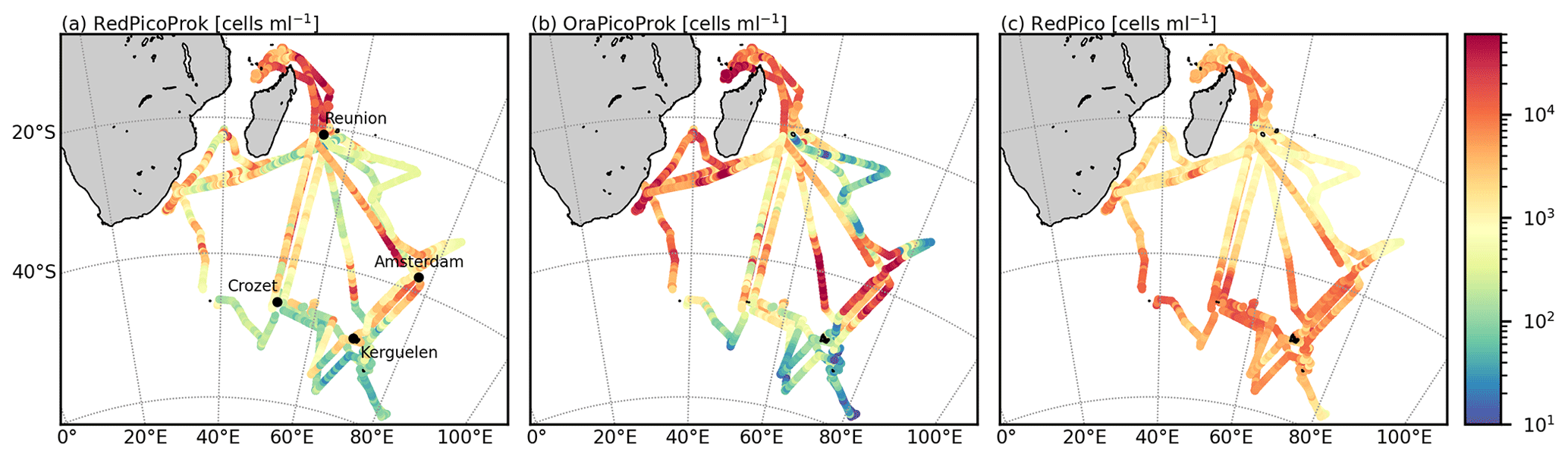
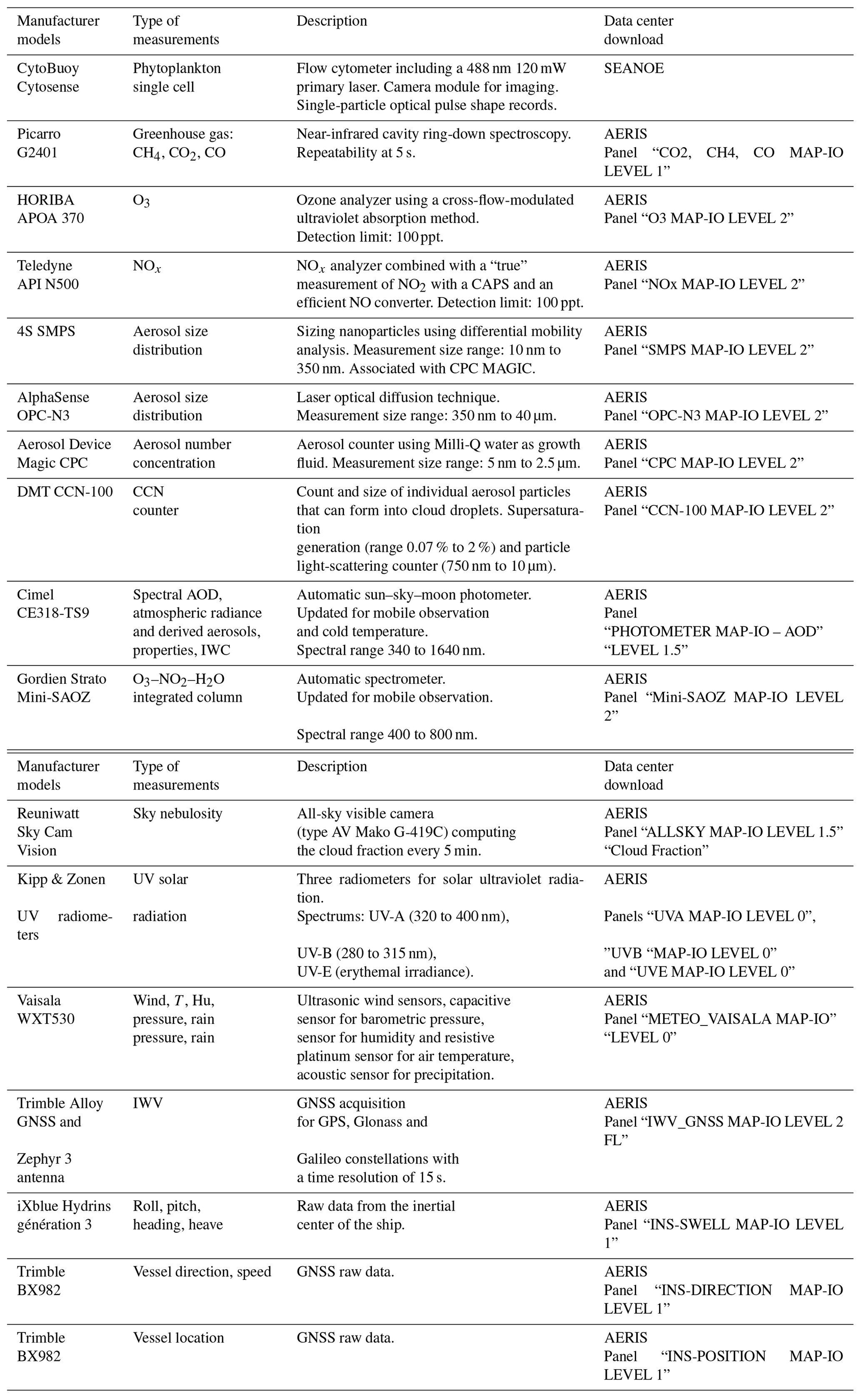
Figure 3 Abundance distributions for samples collected during the 2021–2022 MAP-IO cruises where the Cytosense instrument was in use for (a) RedPicoProk (cells cm⁻³), (b) OraPicoProk (cells cm⁻³), and (c) RedPico (cells cm⁻³). All abundances are available at https://www.seanoe.org/data/00783/89505/ (last access: 8 November 2023). To limit the superposition of the trajectories, they were slightly offset.

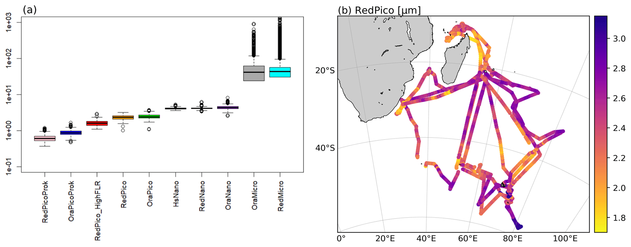
Figure 4 (a) Boxplot of the estimated ESD (µm) for all phytoplankton groups identified, except for OraMicro and RedMicro, where length (µm) is used as they may correspond to chains of cells – from left to right: RedPicoProk, OraPicoProk, RedPico_HighFLR, RedPico, OraPico, HsNano, RedNano, OraNano, OraMicro, RedMicro. (b) Average ESD (µm) distribution for RedPico cells.

Figure 5 Boxplot of the abundance of the phytoplankton groups identified (cells cm⁻³).

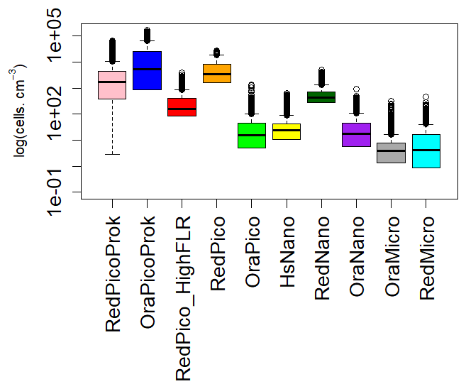
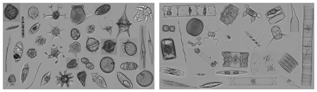
Figure 6 Random collection of phytoplankton pictures from the Cytosense image flow device with a resolution of 3.6 pixels µm⁻¹.

5 Overview of the first results

5.1 Surface phytoplankton distribution

Phytoplankton cells were separated into 10 functional groups identified following the standard vocabulary (Thyssen et al., 2022b), namely, RedPicoProk, OraPicoProk, RedPico, HsNano, OraNano, RedNano, OraMicro, and RedMicro. Samples were collected at a spatial resolution of 14±9 km, and sampled volumes were averaged to 1.04±0.36 cm⁻³ for FLR5, resolving the smallest groups (OraPicoProk, RedPicoProk), and 5.58±1.44 cm⁻³ for FLR20, resolving the other cited groups. Quality-controlling was checked using the referenced 2 µm red polystyrene fluorescing beads, and a maximum deviation of 4 % around the mean of the total FWS was observed. RedPicoProk and OraPicoProk are the most abundant cells counted, with median values of 1730 and 5130 cells cm⁻³ and with maximal values of 66 080 on 21 July 2021 and 161 900 cells cm⁻³ on 19 May 2022, respectively (Fig. 3). The sizes estimated are the smallest within the phytoplankton cells observed with the flow cytometer, with median values of 0.6 and 0.87 µm (Fig. 4), but maximal values reached 1.17 and 1.64 µm, respectively. The RedPico median abundance was 3390 cells cm⁻³, and the maximal value found was 27 250 cells cm⁻³ on 5 May 2022 close to the southwestern African coast, with a median size of 2.33 µm. The other groups' median abundances are below 500 cells cm⁻³ but with inverse ESD values (Figs. 4 and 5). As an example of a finding, there is a significant difference in the RedPico ESD between nighttime and daytime samples, with larger cells during the day than during the night (2.25±0.31 and 2.37±0.30 µm, p<0.001), suggesting the influence of a diel cycle with the majority of smaller divided cells being observed during the night. A significant difference in size between cells north and south of −40° S (2.28±0.30 and 2.43±0.40 µm, p<0.001) also evidences a difference in adaptation to warm subtropical waters and cold subantarctic waters. The average smallest RedPico cells were found during April–May 2022 in the Mozambique Channel (2.15±0.29 µm) and during June and July to the north and northeast of the island of Madagascar. A similar significant trend during the night and day or north and south of −35° S in terms of ESD differences is observed for OraPicoProk and RedPicoProk, while RedNano does not evidence diel or north–south differences. The integrated camera collects photographs of the cells with a resolution that is good enough for identification at a high taxonomic level for cells above 10 µm (Fig. 6). Not all cells are pictured, but there are enough per group of similar pulse shapes. The collected photographs quantify the abundance of the most dominant taxonomic groups observed within the volume sampled. This sampled volume, although taken from less abundant surface waters, still remains enough to picture the diversity of the phytoplankton in southern areas or close to the islands.

5.2 Gas distribution

The time series of CO₂, CH₄, and CO measurements carried out on board the Marion Dufresne from October 2020 to February 2023 are shown in Fig. 7, with measurements from Amsterdam Island as the reference. Unsurprisingly, measurements are highly variable when the ship is in a harbor. There was also a high variability in terms of measurements in the open sea during the RESILIENCE campaign in March–April 2022, which can be explained by the fact that most of the campaign took place in areas fairly close to the coasts of Madagascar and South Africa. On the other hand, the passage close to the TAAF districts had only a very moderate impact on the concentrations of the three gases measured. In these measurement series, episodes of contamination by the ship's chimney were removed based on the detection of CO peak concentrations (El Yazidi et al., 2018) and NO spikes (NO>1 ppb). In total, the NO method leads to the filtering of 15.7 % of the minute-averaged measurements due to local pollution, while the use of CO leads to the elimination of 9.2 % of measurements, about 40 % of which are shared with the NO method. Several high concentrations of CO₂ were thus suppressed, particularly on the transect between Crozet and Kerguelen. The higher frequency of contamination from the ship's stack in this area corresponds to a stronger tailwind. When the Marion Dufresne passes close to Amsterdam Island (less than 5 km), measurements at both sites can be compared. Such comparisons are important to ensure the consistency of the Indian Ocean observation network (Amsterdam, Réunion Island, MAP-IO). The quality-controlling carried out at each site with target gases does not enable the entire measurement chain to be controlled (e.g., possible leak on the sampling line, water vapor correction). Initial comparisons between the Marion Dufresne and Amsterdam Island showed a good correlation between CO₂ and CH₄ measurements, with differences of less than 0.1 ppm and 0.5 ppb, respectively, for CO₂ and CH₄. However, a systematic bias of almost 8 ppb was observed for CO. A re-evaluation of the calibration cylinders used on board the Marion Dufresne was carried out during the OP4 rotation in December 2023. This bias explains the systematic offset observed for CO in Fig. 7. The reactive-gas instruments worked, on average, for 90 % of the measurement days at sea between 2021 and 2023. About 30 % of the data have been filtered due to local pollution, using NO spikes, CO spikes, to confirm local pollution (NO>1 ppb).

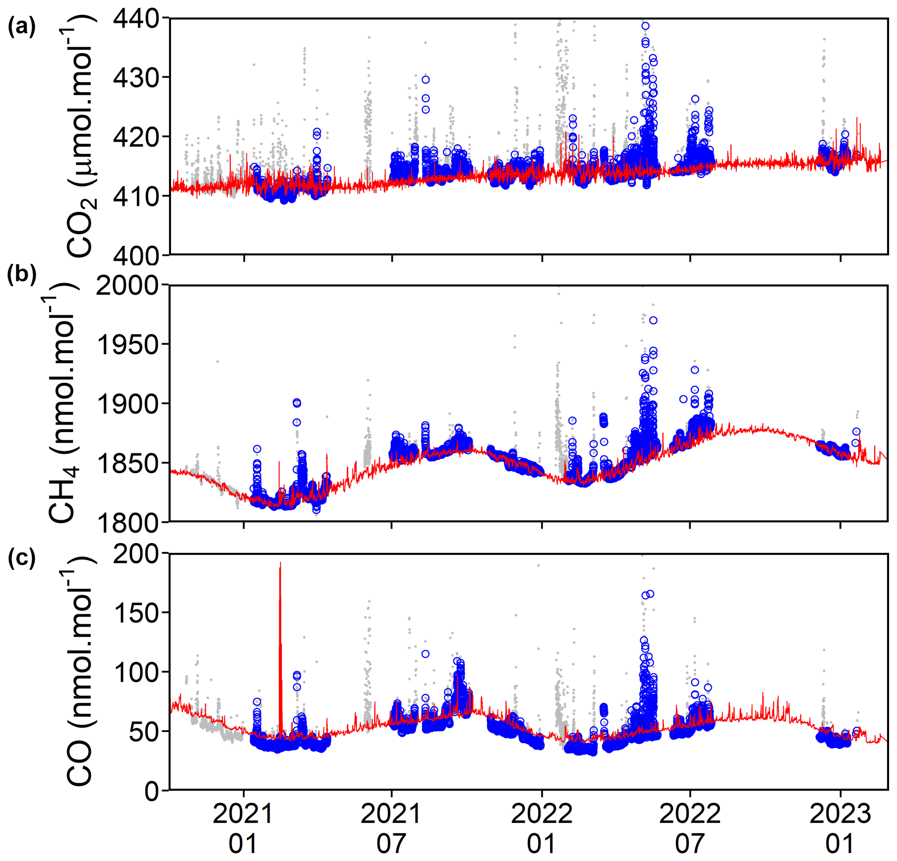
Figure 7 Time series of CO₂, CH₄, and CO concentrations monitored on board the Marion Dufresne (blue circles) compared to the Amsterdam Island observatory (red line). The gray points correspond to measurements made on board Marion Dufresne during stopovers in a port or that were contaminated by the ship exhausts. Each point represents an hourly mean. The CO peak in February 2021 corresponds to a fire on Amsterdam Island.

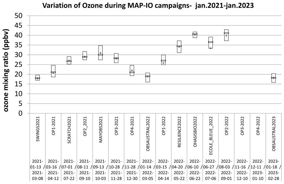
Figure 8 Mean and quartile concentration of ozone (ppb) during the MAP-IO campaigns – January 2021 to January 2023. The names of the campaigns and their respective dates have been entered on the x axis.

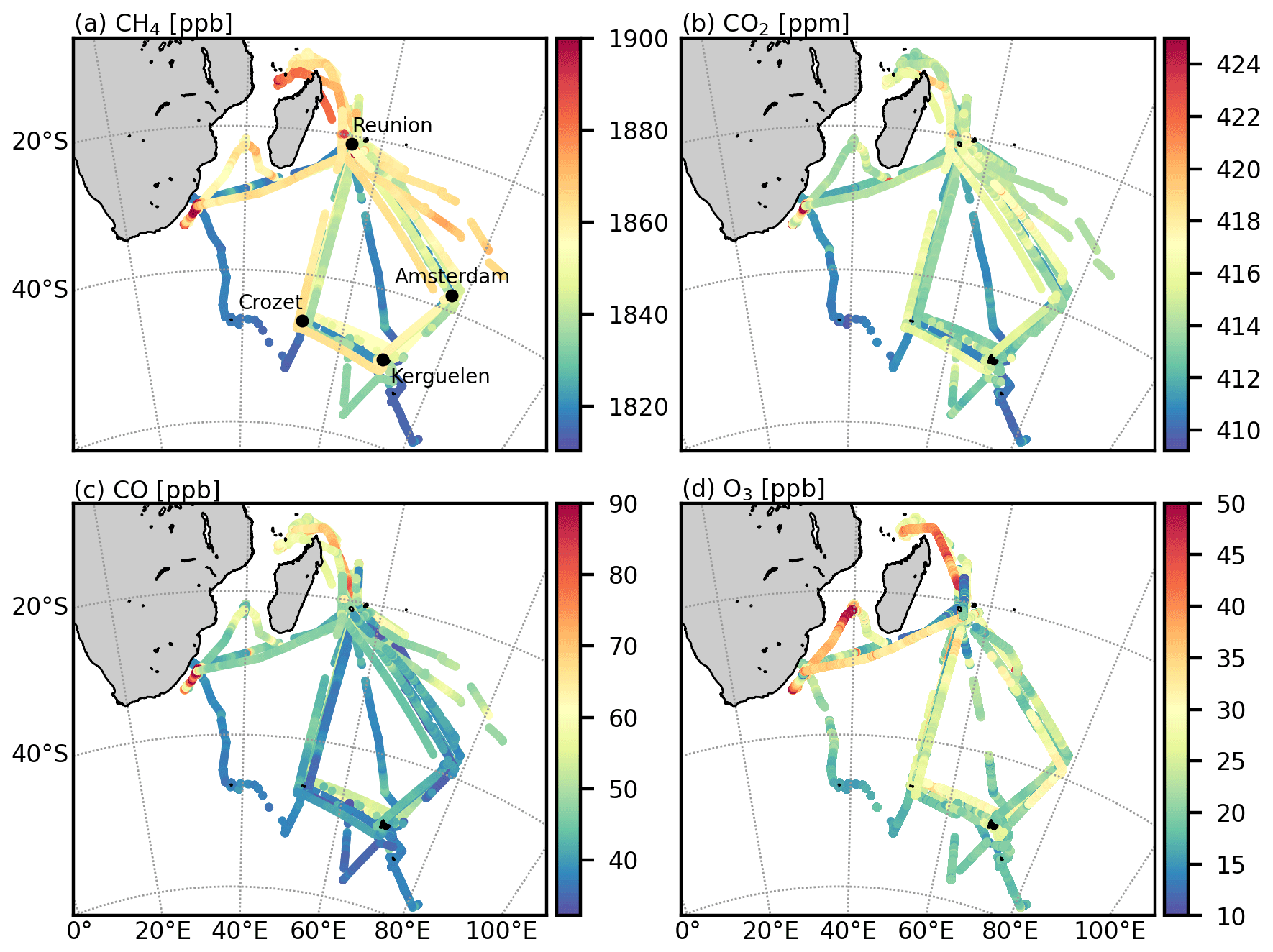
Figure 9 Variation of gaseous species mixing ratios during the 2021–2023 MAP-IO campaigns. The black dots represent the position of Réunion Island, Crozet, Kerguelen, and Amsterdam Island.

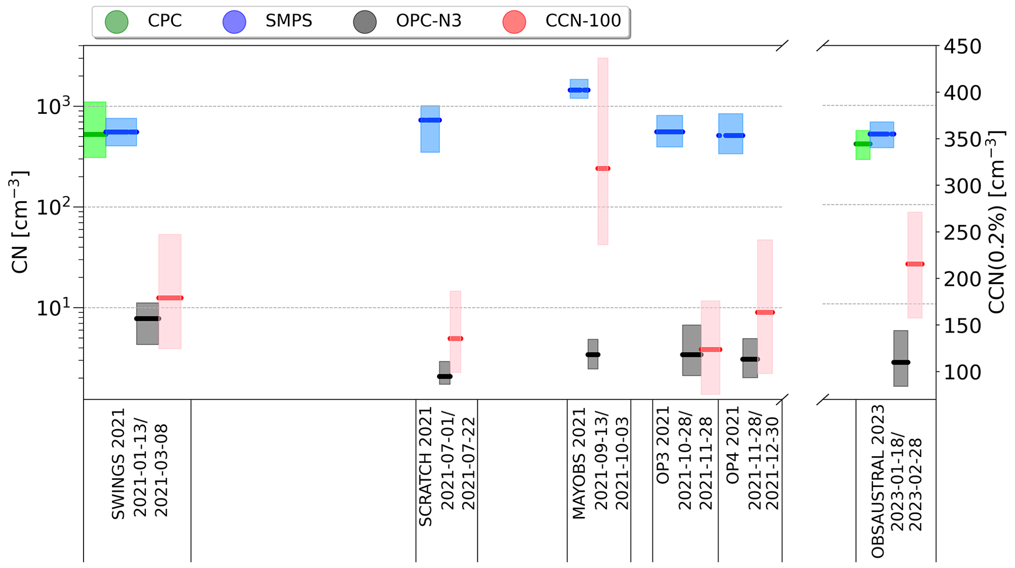
Figure 10 Mean and quartile concentration of aerosols (in cm⁻³, scale on the left) measured by the SMPS (blue), CPC (green), and OPC-N3 (black). The CCN at 0.2 % supersaturation measured by the CCN-100 was superimposed (in cm⁻³, scale on the right). The names of the campaigns and their respective dates have been entered on the x axis.

The ozone seasonal variation (Fig. 8) shows a minimum (∼18 ppb) in summer (January) and a maximum (between 30 and 40 ppb) during the winter season. This seasonal variation and associated ozone mixing ratios are in good agreement with the few ozone measurements performed in the remote mid-latitude Southern Hemisphere, on Amsterdam Island (Gros et al., 1998), and in Cape Grim (Parrish et al., 2016). In particular, the seasonal variation observed in 2022 (with a maximum of 30 ppb) is very similar to the mean seasonal cycle from the long time series obtained at Cape Grim since 1982 (Schultz et al., 2017), showing the representativeness of these measurements for this region. The higher winter values measured during 2022 correspond to campaigns performed at latitudes higher than 30° S and may have been influenced by the impact of biomass burning, which is active in southern Africa during the May–November period. The same seasonal behavior is clearly seen for CH₄ and CO (Fig. 7), with a minimum observed in summer (February–March) due to the photo-oxidation of this species (OH sink). The high concentrations of CH₄, CO, and CO₂, observed in winter 2022, confirm the continental origins of this anomaly. It is also important to note the strong increase in CH₄ (by about 21 ppb) between summer 2021 and summer 2022, in line with measurements taken on Amsterdam Island and at other observatories (Lin et al., 2023). The spatial variability of reactive gases is shown in the trajectories of the Marion Dufresne in Fig. 9. It is important to note that this representation also incorporates the seasonal variability. As expected, the highest concentrations are generally measured near continents. High concentrations were measured on the road north of Madagascar (CH₄∼1850 ppb, CO₂∼415 ppb, CO∼70 ppb, and O₃∼40 ppb) or, more occasionally, off the coast of South Africa (CH₄∼1900 ppb, CO₂∼420 ppb, CO∼90 ppb, and O₃∼45 ppb). The low concentrations are spatially more variable and probably linked to meteorological conditions. In pristine conditions, the lowest concentrations reached in 2021 were 1800, 410, 30, and 10 ppb, respectively, for CH₄, CO₂, CO, and O₃. As expected, the most reactive species (O₃, CO) present a more pronounced spatial variability than for the greenhouse gases CO₂ and CH₄. We also note in Fig. 9 the high and continuous concentrations of CO (>50 ppb) and ozone (>25 ppb) on certain paths far from the main anthropogenic sources. As there are no CO emissions over the ocean, these high concentrations are attributed to long-range transport, usually of biomass burning plumes. For example, on the Crozet–Kerguelen route of the SWINGS campaign, several concentration peaks were detected between 11 and 17 February 2021 – i.e., an increase in CH₄ of around 6 to 12 ppb, an increase in CO of 5 to 10 ppb, and an increase in CO₂ of 10 to 20 ppm.

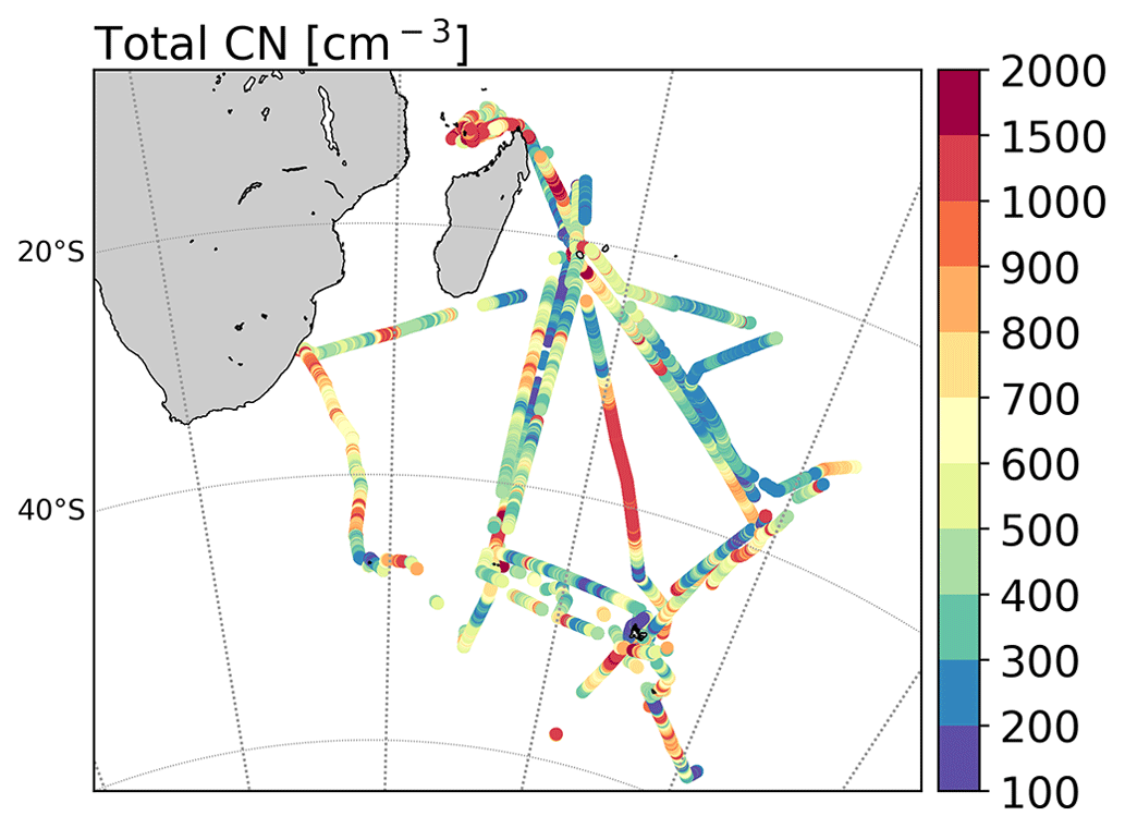
Figure 11 Evolution of the total number of aerosols (CN in cm⁻³) along the path of the Marion Dufresne over the year 2021 and between January and March 2023. Note that the SMPS was undergoing maintenance in 2022. The discontinuous zones correspond to the filter on the relative wind (from rear direction or at low speed) or during stops made by the ship in order to eliminate any risk of contamination by the ship's exhaust or by the activity on board. To limit the superposition of the trajectories, they were slightly offset.

5.3 Atmospheric aerosols

5.3.1 In situ aerosols

Figure 10 shows the mean and quartiles of aerosol and CCN concentrations measured by the CCN-100, SMPS, OPC-N3, and CPC during the various campaigns in which the instruments operated normally. The mean total aerosol number concentration varied between 530 cm⁻³ (average during OBSAUSTRAL in January–February 2023) and 1500 cm⁻³ (average during MAYOBS in September 2021) (Fig. 10), which is consistent with the orders of magnitude reported in the literature for marine regions under the clean air masses of the Southern Hemisphere (Humphries et al., 2021; Sellegri et al., 2023). In the coarse mode (OPC-N3), 50 % of the 1–10 µm particle concentrations are in the range 1–12 cm⁻³.

We note a strong spatial variability in terms of the aerosol concentration, with low concentrations on the northeastern parts of the ship's track (Fig. 11) and higher concentrations north of Madagascar (concentration reached 2000 cm⁻³) and in the center the Indian Ocean between Kerguelen and La Réunion (mean concentration at 1100 cm⁻³). The high concentrations observed north of Madagascar correspond to the high CO and O₃ concentrations also observed (see Sect. 4.2), pointing to potential terrestrial outflows, but they also match with high concentrations of CH₄ and picophytoplankton cell abundances; therefore, a biological influence can not be excluded. Below the latitude of 40° S, the total aerosol concentration is also spatially variable, probably linked to a greater variability in terms of meteorological conditions (storms and strong swells) and potentially also due to a high variability in terms of phytoplankton concentrations in the Subantarctic Front region (Fig. 3) that need further investigation.

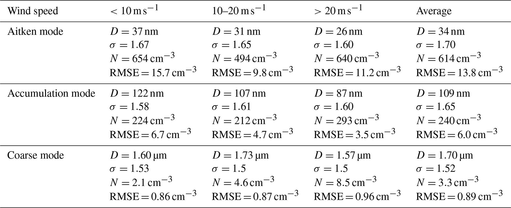
Figure 12 shows the particle size distribution of the aerosols throughout the measurement period, fitted by log-normal functions (size ranges 20–350 nm and 400 nm–6 µm) in three modes classically observed in the atmosphere, corresponding to the Aitken, accumulation, and coarse modes. The calculated median diameters are 34 nm, 109 nm, and 1.7 µm, and the standard deviations are 1.7, 1.65, and 1.52 for the Aitken, accumulation, and coarse modes, respectively (Table 2). A second coarse mode can also be observed at 4.5 µm but is at the limit of validity of OPC-N3. Similarly, there may be a second undetected accumulation mode between 300 nm and 400 nm due to instrumental limitations. The size distributions were then separated based on the wind speed measured on the ship. At a wind speed less than 10 m s⁻¹, the primary marine aerosol emission is considered to be low, in the range 10–20 m s⁻¹; the primary emission becomes significant; and for storms (>20 m s⁻¹), very few observations have been made on ships (e.g., Ovadnevaite et al., 2014; Bruch et al., 2021). The submicronic aerosol concentration is significantly lower for moderate wind conditions (10–20 m s⁻¹). For the coarse mode, concentrations are 4 times higher for strong winds (>20 m s⁻¹) than for low winds (<10 m s⁻¹), which is in line with the production of primary marine aerosols by wave breaking.

The median diameters of the Aitken and accumulation modes decrease with the wind speed. Part of this result can be attributed to primary emissions which counterbalance the aerosol growth process during the aging of the air mass by the formation of new smaller particles. Therefore, it will be relevant to look for factors other than wind speed (SST, precursor gases, aerosol wash-out along the back-trajectory path, etc.) which significantly influence emissions, formation, and growth of submicron aerosols.

The mean CCN concentration at 0.2 % supersaturation (CCN_0.2) ranged between 125 cm⁻³ (OP3, October 2021) and 320 cm⁻³ (MAYOBS, September 2021). The variability is particularly important in relation to CCN concentrations, with 25 % of the concentrations being lower than 50 cm⁻³ in October 2021 and higher than 440 cm⁻³ during September 2021. We also note that, for campaigns with similar routes, the average CCN_0.2 $/$ CN ratios, which are a function of aerosol size and composition, can be very different from one campaign to the other while being measured during the same season. For example, the ratio was 0.20 for October–November 2021 and 0.45 for January–February 2023, showing the important variability of the aerosol hygroscopicity.

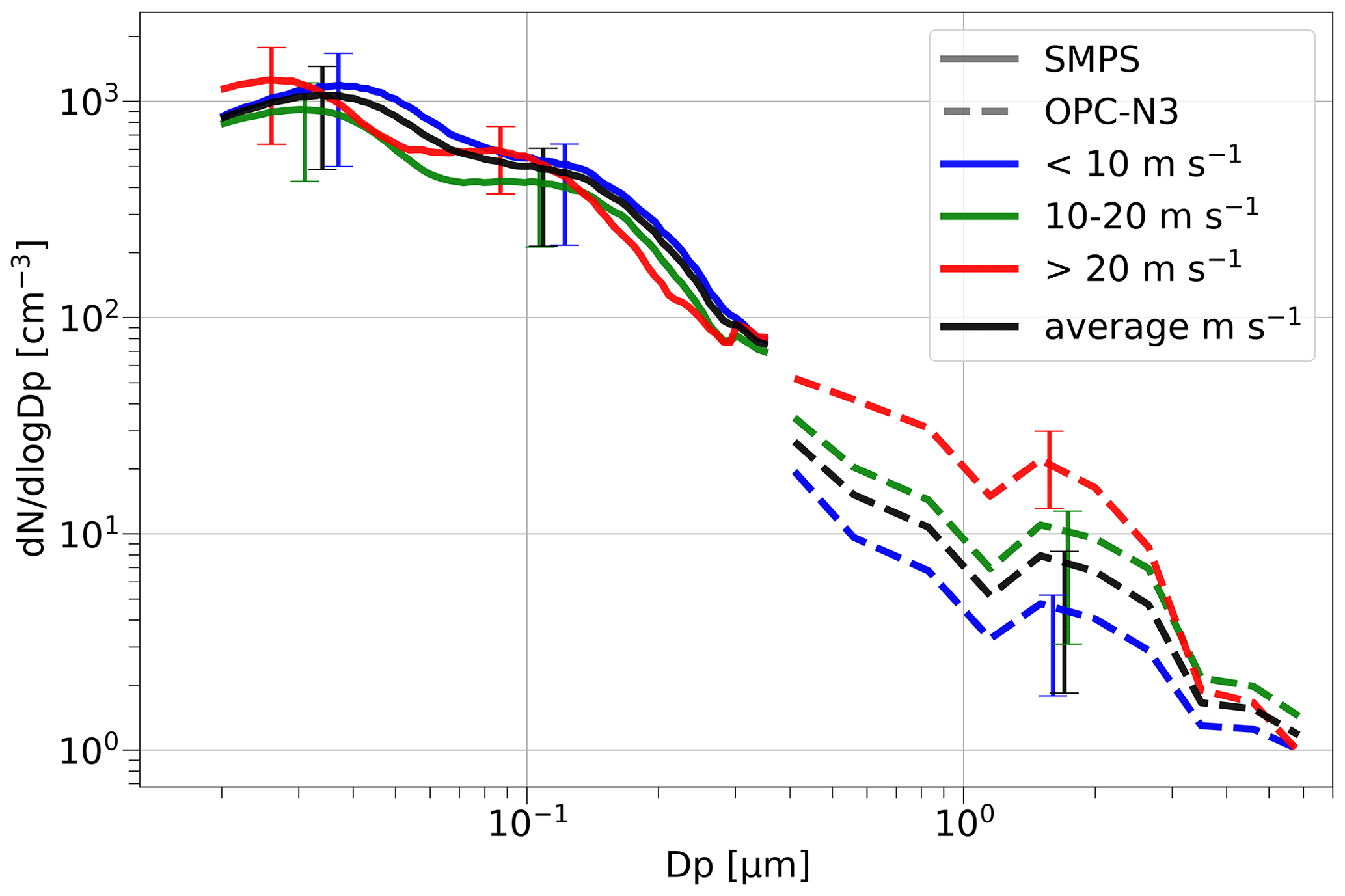
Figure 12 Aerosol size distribution and root mean square deviation observed during 2021 and between January and March 2023 by the SPMS and OPC-N3. Vertical lines correspond to the quartile concentration measured at the bin corresponding to each mean diameter of the log-normal functions.

Table 2 Aerosol size distribution of each mode fitted into a log-normal distribution (total number (N), mean diameter (D), standard deviation (σ), and root mean square error (RMSE).

5.3.2 Aerosol (remote sensing)

From early July 2021 to early May 2022, ∼10 000 cloud-free AODs (level 1.5) were recorded. In cloud-free conditions, AODs are measured every 15 and 3 min during the daytime (70 % of records) and the nighttime (30 % of records), respectively. The mean AOD is 0.095±0.070, 0.086±0.05, and 0.060±0.03 at 440, 500, and 870 nm, respectively. The mean Angström exponent (AE), computed between 440 and 870 nm, is 0.7±0.3, and the mean water vapor content is 2.8±1.1 g cm⁻¹. The average AOD is very consistent with Mallet et al. (2018). Overall, the values of AE range from about 0.0 to ∼1.5, with a mean of ∼0.7. Such values are typical of marine aerosols and are consistent with Mallet et al. (2018) and also with Smirnov et al. (2002), who report AE values ranging from 0.3 to 0.7 over clean marine regions free of continental influences. In the following, we address the spatial variability, in terms of latitudinal variation, for the AOD, AE, and water vapor. For that purpose, we average all the data recorded within a 1° latitude grid (Fig. 13). For the sake of clarity, we organized the results by season, labeled DJF (December to February), MAM (March to May), JJA (June to August), and SON (September to November). Clear decreasing trends are observed from the northern part to the remote southern part of the Indian Ocean for AOD and water vapor. This is observed for all seasons. The reported AOD values are consistent with the results from Mallet et al. (2018), derived in the southern Indian Ocean. An interesting behavior is the separation of relatively low AOD (lower than 0.075) and relatively high AOD (>0.08), which occurs around 35° in latitude in DJF, 25° in MAM, 20° in JJA, and 30° in SON. This latitudinal behavior suggests that this separation follows the motion of the intertropical convergence zone (ITCZ). According to Mallet et al. (2018), the relatively low AOD values reflect the presence of sea salt, while the higher values are more typical of sulfate. These values are also consistent with those reported by Mascaut et al. (2022) around Réunion Island. The same comment can be made for the Angström exponents, whose values are typical of marine aerosols. The increase in absolute humidity with the latitude is not surprising as one travels closer and closer to the Equator. These first results are also consistent with those obtained during the AEROMARINE field campaign around Réunion Island (Mascaut et al., 2022).

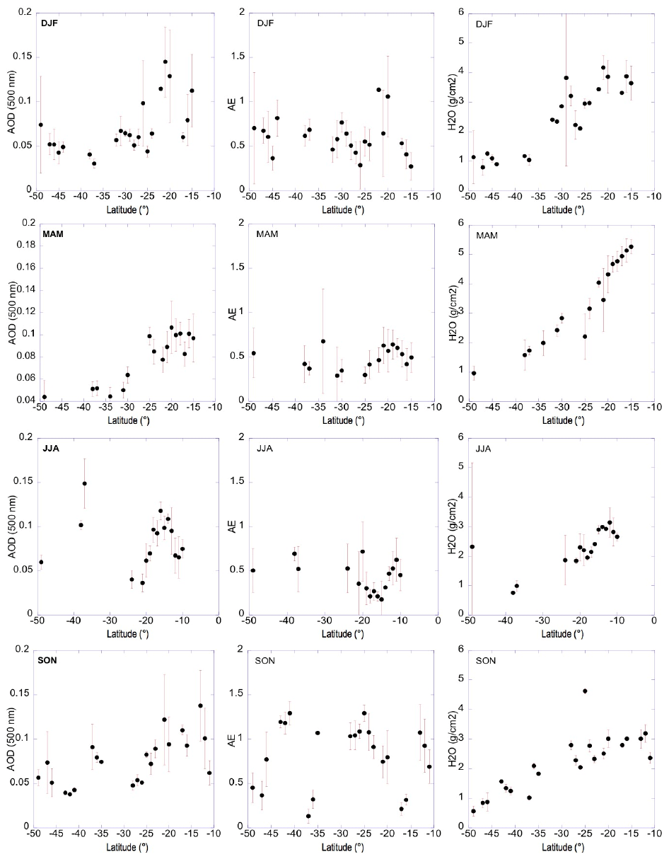
Figure 13 Latitudinal variation of AOD (a), Angström exponent (b), and water vapor content (c) for each season (DJF, MAM, JJA, SON). The observations considered here are coming from both daytime and nighttime records. “Error bars” stand for the standard deviation of the corresponding properties within the 1° latitude grid.

5.4 Comparison of IWV (GNSS, SAOZ, photometer)

Water vapor, a key climatic constituent, is a challenging variable to measure due to its spatial and temporal variability (Bock et al., 2013). The integrated vertical column of water vapor can be assessed by different instruments co-located on board the Marion Dufresne. The GNSS instrument performs measurements over a large atmospheric cone above an elevation on the horizon of 3° over the whole sky covered by GPS satellites (360°) (Bosser et al., 2022). Other instruments are a UV–Vis Mini-SAOZ spectrometer and a sun photometer. The predecessor of Mini-SAOZ showed consistency with GNSS observations during the DEMEVAP campaign in September–October 2011 in the Northern Hemisphere mid-latitude station of OHP (Observatoire de Haute Provence) in France (Bock et al., 2013). Mini-SAOZ measures a slant column that changes as a function of the sun's position. The spatial extent of air masses sampled by the Mini-SAOZ could be associated with a 2-D polygon projected to the surface (Garane et al., 2019). Vertical columns are obtained and then divided by the corresponding AMF for H₂O. Only observations at a SZA lower than 60°, sensitive to tropospheric constituents, are used in this study. Measurements presenting a computed color index (ratio of the fluxes at 550 and 350 nm already corrected from constituents) higher than 5 were filtered. In the case of the photometer, this performs direct sun and moon measurements. The air masses sampled by the instrument correspond to a column in the direct direction between the sun or the moon and the instrument. Figure 14 (top panel) shows the time evolution of IWV observed by the GNSS (black points), the Mini-SAOZ (red points), and the sun photometer (blue points) during the Marion Dufresne trips. Despite the three instruments' different sampling geometries corresponding to somewhat different atmospheric H₂O amounts, their observations clearly show a strong agreement. The evolution of IWV is also correlated with the latitude of the ship (bottom panel of Fig. 14). Large amounts of IWV are observed when the ship travels in tropical regions at an equatorward latitude of 25° S, with a mean value of 8.5±2.1 (1σ) $\mathrm{molec}.{\mathrm{cm}}^{-\mathrm{2}}$, while mean values 2 to 3 times weaker are observed at a poleward latitude of 45° S over the Indian Ocean. Figure 15 presents the zonal mean IWV value and ±σ observed by the three instruments between 60 and 10° S. The latitudinal gradient of IWV is well highlighted by each instrument. A good agreement within 1σ is found between the measurements, with a higher latitudinal amplitude for SAOZ IWV.

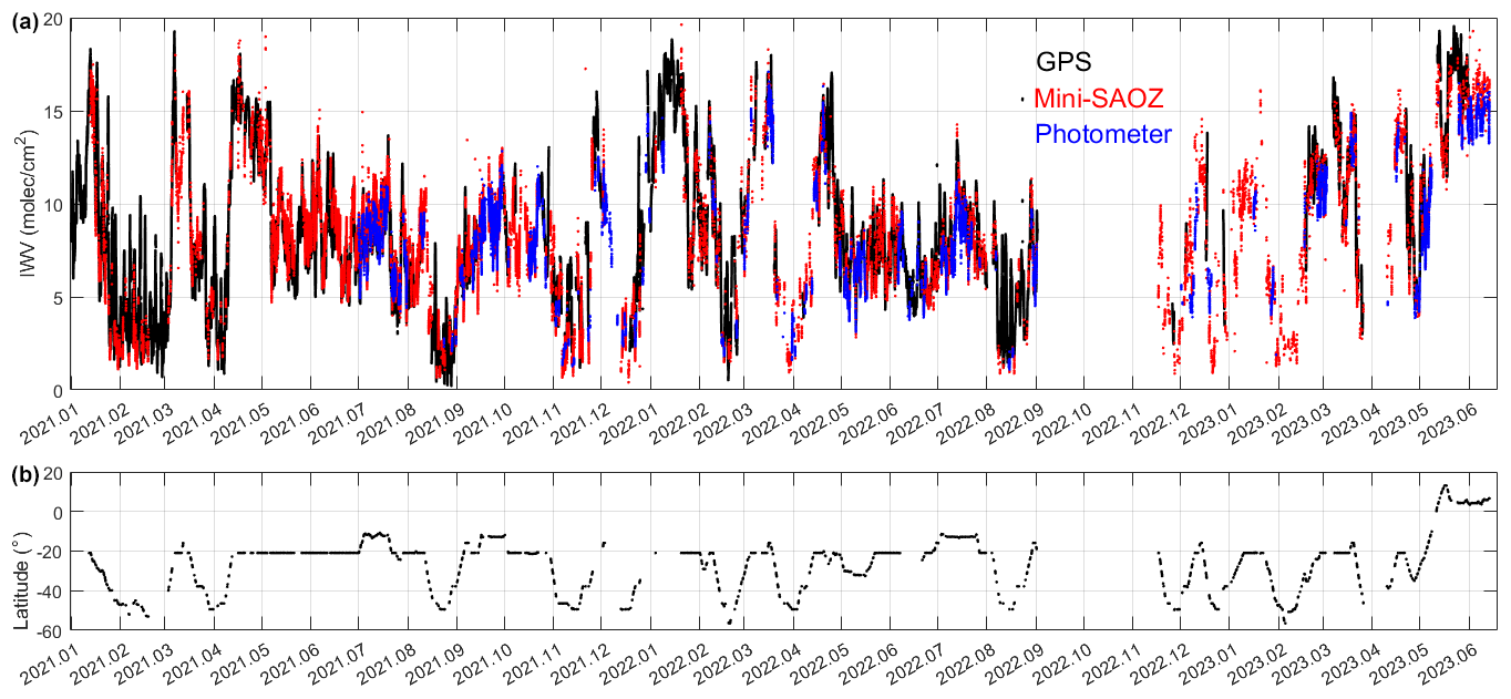
Figure 14 Evolution of integrated water vapor observed by GNSS (GPS), Mini-SAOZ, and photometer since January 2021 (a). Latitude of the Marion Dufresne (b). The interruption of measurements at the end of 2022 corresponds to the technical stop of the vessel in Singapore.

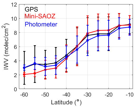
Figure 15 Zonal IWV mean ±1σ observed by GNSS (GPS), Mini-SAOZ, and photometer instruments on board the Marion Dufresne. GNSS and photometer data were sampled at Mini-SAOZ time.

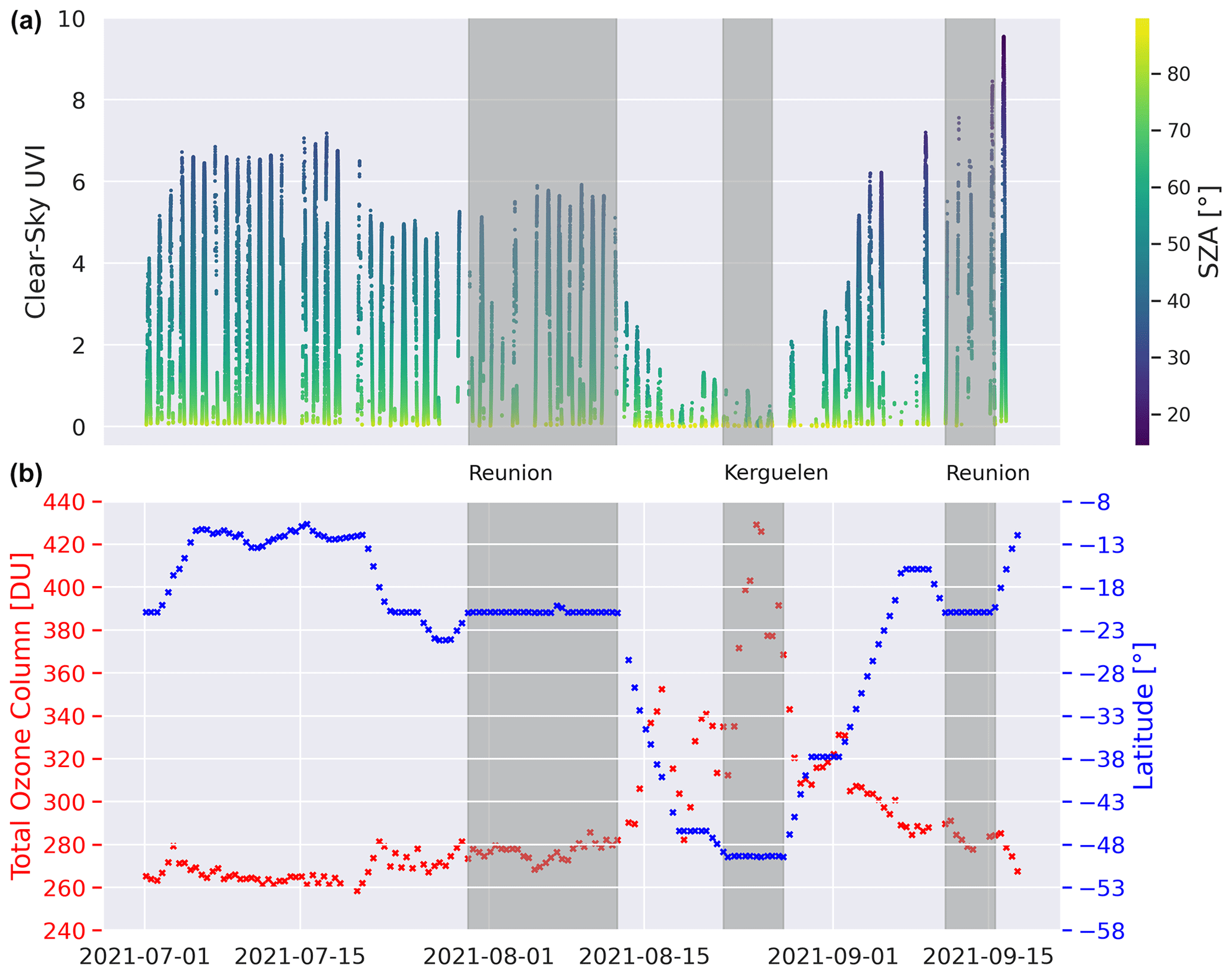
Figure 16 Daily clear-sky UV-E from SUV-E radiometer with color code indicating the SZA (a) and twilight total ozone column and latitude from Mini-SAOZ instrument (b) between 1 July 2021 and 15 September 2021. The gray zones indicated the period where the Marion Dufresne ship was at the Réunion and Kerguelen stations.

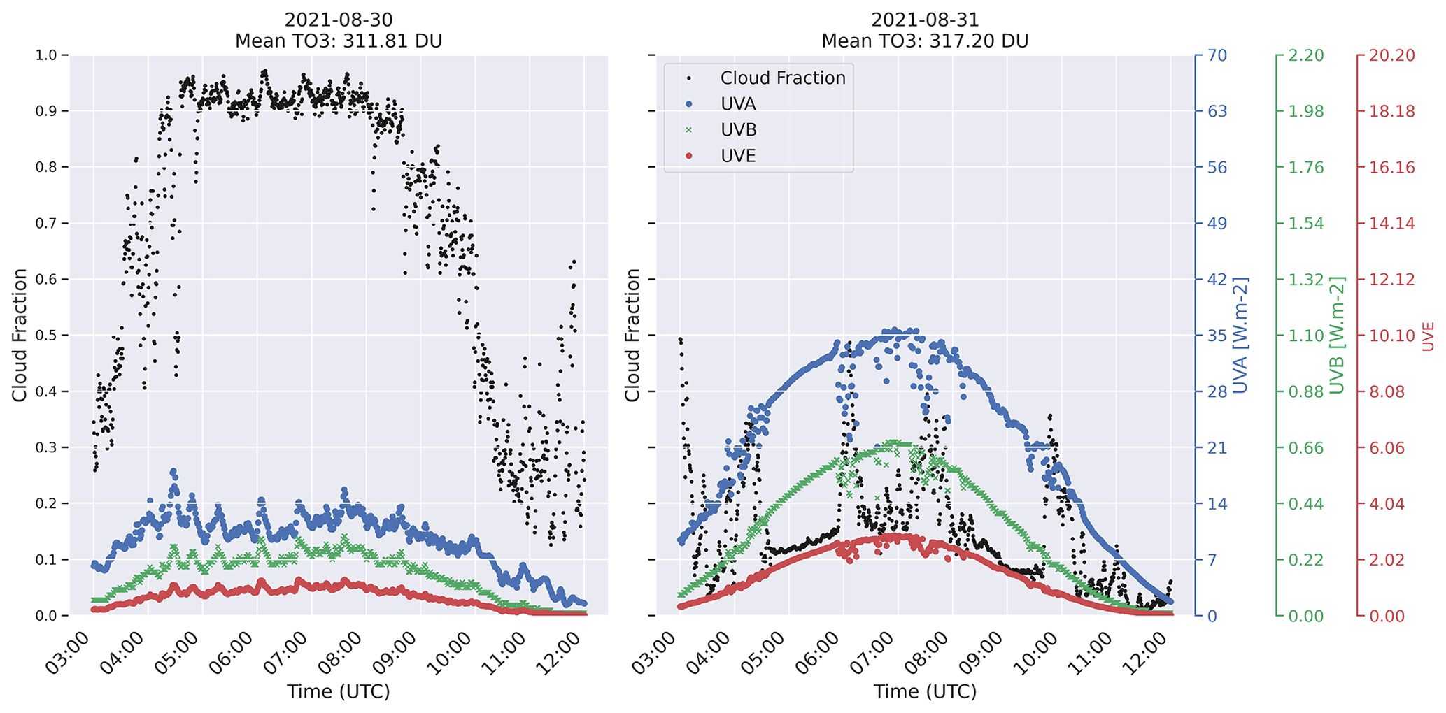
Figure 17 UV-A, UV-B, UV-E, and cloud fraction measurements taken on the days of 30 and 31 August 2021.

5.5 UV and stratospheric ozone

The UV erythemal index (UV-E) measured by the SUV-E radiometer under clear-sky conditions is shown in Fig. 16. These conditions were identified based on cloud fraction measurements captured by the sky camera and a previously optimized cloud fraction threshold for other sites in the southwestern Indian Ocean region (Lamy et al., 2021b). A color code is utilized to signify the variable solar zenith angle. The total ozone column, derived from the Mini-SAOZ instrument, and the latitudinal variation are portrayed in red and blue, respectively. As the vessel moves poleward from Réunion to Kerguelen, the latitude changes from approximately 20° S to about 48° S, and the daily minimum solar zenith angle values reached are higher at higher latitudes, visually represented in Fig. 16 by a gradient line color that shifts towards yellow as the solar zenith angle values increase. Conversely, the daily minimum solar zenith angle values decrease when the vessel travels toward the Equator – or, in other words, the sun's highest point in the sky goes to the zenith near 20° SZA as the vessel travels toward the Equator. There is a notable decrease in UV observed in conjunction with the movement towards higher latitudes (from Réunion to Kerguelen). This is anticipated to be inversely correlated with the increase in the total ozone column, generally noted in middle and high latitudes due to the BDC.

The measurements of UV-A, UV-B, and UV-E radiation taken by the radiometers SUV-A, SUV-B, and SUV-E on 30 and 31 August 2021 are illustrated as blue, green, and red dots, respectively, in Fig. 17. The cloud fractions, measured by the camera, are also denoted by black points. The mean daily values of total ozone were similar for both days at 311.81 DU (Dobson units) on 30 August and 317.20 DU on 31 August. However, the cloud fraction diurnal values presented significant disparities. Given the proximity in total ozone values, one might expect similar measurements of UV radiation for both days. However, this was not the case due to the large variations in cloud conditions. On 30 August, the day was predominantly overcast, with high cloud fraction (CF) values persisting between 03:00 and 09:00 UTC. Conversely, 31 August was a partially clear day, characterized by intermittent low to moderate CF values (between 0.1 and 0.5) around 03:00, 04:00, 06:00, and 08:00. During phases of very low cloudiness, UV radiation increases until solar noon time (lowest solar zenith angle of the day) and then decreases, thus producing a bell-shaped curve. An increase in CF values to approximately 0.5 on 31 August, particularly around 06:00 and 08:00 (close to local solar noon), was anti-correlated with a decrease in UV-A, UV-B, and UV-E values. High CF values on 30 August were associated with substantial attenuation of UV-A, UV-B, and UV-E radiation throughout the day. UV-B is less affected by clouds than UV-A due to the spectral dependence of clouds transmittance. Past research has shown that cloud transmittance is higher for UV-B than for UV-A by approximately 60 % and 40 %, respectively (Seckmeyer et al., 1996).

6 Data availability

Atmospheric data are available from the AERIS data center: https://www.aeris-data.fr/catalogue-map-io/ (last access: 8 November 2023). Cytometry data are available from the SEANOE data center: https://doi.org/10.17882/89505 (Thyssen et al., 2022a).

7 Conclusions

The purchase and deployment of the instrumentation on the vessel took place between September 2020 and January 2021. Despite all the often complex operational and technical difficulties to be resolved on an oceanographic vessel (i.e., mechanical, instrumentation, IT, work on the ship's hull) and the difficult context of the COVID pandemic (PPE equipment, limited contact with sailors on board), nearly 700 d of observations at sea were carried out between January 2021 and June 2023.

The first climatological studies based on the database show significant intra-seasonal and latitudinal variabilities in terms of greenhouse gases concentration and aerosol optical depth. The total number, the size distribution, and the CCN properties of aerosols vary considerably depending on the air masses sampled (from 100 to 1000 particles cm⁻³). It can be seen that the average CCN_0.2 $/$ CN ratios vary significantly for a given geographic location and season, reflecting important variations in the hygroscopic and/or size distribution of the aerosols measured. The first rough level of investigation of the factors influencing the aerosol concentration and size shows that wind speed explains a significant part of the coarse-mode aerosol concentrations, but other factors are needed to explain the submicron aerosol concentrations.

The phytoplankton community structure has been studied by resolving several size classes, and the collected data set can be considered to be one of the most important data sets of surface phytoplankton abundance collected so far in such a short time and in this remote area. The single-cell study evidenced physiological and possible taxonomic differences following latitudes more than seasons according to the shift in size per functional phytoplankton group resolved. A deeper study into the contribution of each group to chlorophyll A and carbon will enhance the understanding of the role of phytoplankton in sustaining biogeochemical cycles and the trophic web. Further insight into this representative ocean–atmosphere data set will open the path to some strong statistical relationships that would raise new scientific questions.

The collection of the in situ data of MAP-IO under different latitudes and seasons, sea states, and meteorological conditions should provide an original framework for studying and improving the parameterizations of turbulent fluxes at the surface. For example, machine learning methods exploiting large databases could be used. In this context, the vast instrumental setup installed on board to characterize the properties of aerosols, trace gases, and phytoplankton classes should allow us to evaluate and improve the parameterization of ocean–atmosphere exchanges, especially under strong winds and high swell conditions. Integrated optical depth measurements of ozone, UV, and aerosols over the Indian and Southern Ocean can be integrated for the calibration–validation of the European mission EARTHCARE (including the ATLID lidar and MSI spectrometer); the USA AOS mission (Atmosphere Observing System, including polarimeter, lidar, and water vapor sounder); the European EPS-SG missions (EUMETSAT Polar System – Second Generation, which will include the 3MI polarimeter, IASI-NG, and METimage radiometer); and Sentinel-2, Sentinel-3, and Sentinel-5P by sampling different atmospheric conditions. Measurements by class of phytoplankton will make it possible to contribute to a better plankton functional group community structure quantification by means of dedicated remote sensing ocean color products (Uitz et al., 2006; Alvain et al., 2008; El Hourany et al., 2019) (e.g., OLCIA, OCLIB, GlobColour) over the Indian and Southern oceans.

Several innovations have been developed, including the development of fast GNSS zenith delay inversion algorithms for integrated water vapor content restitution for integrating the specificities of ship movements. Adaptations to make the CE318T lunar–solar photometer autonomous and adapted to heavy swells and icing were also developed. The Mini-SAOZ, successfully tested for the first time on a ship, also enabled continuous acquisition of integrated water vapor and ozone columns over the ocean. These three instruments provide reliable, continuous, and local measurements of atmospheric water vapor in regions where the main source of observations is space-based. This measurement, performed routinely with low latency, could contribute to the evaluation of, or even assimilation into, numerical weather models. Long-term monitoring of the spatial and temporal distributions of water vapor could contribute to the monitoring of climate change in these regions.

Test campaigns for onboard instruments, such as the CE370 micro-lidar during the AMARYLLIS-AMAGAS campaign, demonstrated the potential for the permanent deployment of active remote sensing instruments on ships. Generally speaking, the majority of instruments have operated autonomously or with limited human intervention. Many of the data can be transferred within 10 min and thus open up the prospect of near-real-time operation. These successful proofs of concept open up interesting prospects for the development of operational observations both for international research networks such as AERONET or NDACC and for operational numerical forecasting networks. If pursued over future years, the MAP-IO program could be a useful tool for monitoring climate trends and for calibrating and validating numerical forecasting models and space sensors in a region almost devoid of observations.

Appendix A: MAP-IO instrumentation on board

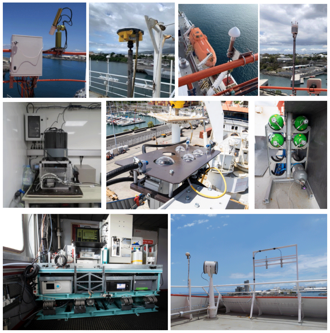
Figure A1 Images of the different instruments on board. Top: photometer, GNSS antenna, Mini-SAOZ, and the meteorological station. Middle: flow cytometer, all-sky camera and UV radiometers, and calibration gas bottles. Bottom: gas and aerosol analyzers on the vibration-dampened table and inlets on deck I. Photography credits: Thierry Portafaix, François Rigaud-Louise and Jean-Marc Metzger.