the Creative Commons Attribution 4.0 License.
the Creative Commons Attribution 4.0 License.
 | 26 Jun 2024
First release of the Pelagic Size Structure database: global datasets of marine size spectra obtained from plankton imaging devices
Marco Corrales-Ugalde
Todd D. O'Brien
Jean-Olivier Irisson
Fabien Lombard
Lars Stemmann
Charles Stock
Clarissa R. Anderson
Marcel Babin
Nagib Bhairy
Sophie Bonnet
Francois Carlotti
Astrid Cornils
E. Taylor Crockford
Patrick Daniel
Corinne Desnos
Laetitia Drago
Amanda Elineau
Alexis Fischer
Nina Grandrémy
Pierre-Luc Grondin
Lionel Guidi
Cecile Guieu
Helena Hauss
Kendra Hayashi
Jenny A. Huggett
Laetitia Jalabert
Lee Karp-Boss
Kasia M. Kenitz
Raphael M. Kudela
Magali Lescot
Claudie Marec
Andrew McDonnell
Zoe Mériguet
Barbara Niehoff
Margaux Noyon
Thelma Panaïotis
Emily Peacock
Marc Picheral
Emilie Riquier
Collin Roesler
Jean-Baptiste Romagnan
Heidi M. Sosik
Gretchen Spencer
Jan Taucher
Chloé Tilliette
Marion Vilain
In marine ecosystems, most physiological, ecological, or physical processes are size dependent. These include metabolic rates, the uptake of carbon and other nutrients, swimming and sinking velocities, and trophic interactions, which eventually determine the stocks of commercial species, as well as biogeochemical cycles and carbon sequestration. As such, broad-scale observations of plankton size distribution are important indicators of the general functioning and state of pelagic ecosystems under anthropogenic pressures. Here, we present the first global datasets of the Pelagic Size Structure database (PSSdb), generated from plankton imaging devices. This release includes the bulk particle normalized biovolume size spectrum (NBSS) and the bulk particle size distribution (PSD), along with their related parameters (slope, intercept, and R2) measured within the epipelagic layer (0–200 m) by three imaging sensors: the Imaging FlowCytobot (IFCB), the Underwater Vision Profiler (UVP), and benchtop scanners. Collectively, these instruments effectively image organisms and detrital material in the 7–10 000 µm size range. A total of 92 472 IFCB samples, 3068 UVP profiles, and 2411 scans passed our quality control and were standardized to produce consistent instrument-specific size spectra averaged to 1° × 1° latitude and longitude and by year and month. Our instrument-specific datasets span most major ocean basins, except for the IFCB datasets we have ingested, which were exclusively collected in northern latitudes, and cover decadal time periods (2013–2022 for IFCB, 2008–2021 for UVP, and 1996–2022 for scanners), allowing for a further assessment of the pelagic size spectrum in space and time. The datasets that constitute PSSdb's first release are available at https://doi.org/10.5281/zenodo.11050013 (Dugenne et al., 2024b). In addition, future updates to these data products can be accessed at https://doi.org/10.5281/zenodo.7998799.
- Article
(6855 KB) - Full-text XML
- BibTeX
- EndNote


1.1 The relevance of plankton size in approximating ecological processes
Plankton size structure observations are essential to bridge the gap between marine biogeochemical processes and biological stock assessments, including those of important commercial species (Boyd and Newton, 1999; Armstrong et al., 2001; Finkel et al., 2009; Guidi et al., 2009; Taniguchi et al., 2014; Hillebrand et al., 2022). Historically, ecosystems dominated by small phytoplankton were thought to support regenerated production, being rapidly recycled in the epipelagic layer and contributing little to carbon export. Conversely, larger phytoplankton were thought to fuel higher trophic levels and contribute, to a large extent, to carbon sequestration by sinking relatively fast to the mesopelagic (200–1000 m) layers (Legendre and Le Fèvre, 1995; Wassmann, 1997; Durkin et al., 2015). Although this paradigm has shaped almost all current biogeochemical models and their projections of marine ecosystem services under climate change, recent studies have challenged this concept. Indeed, plankton of intermediate size and/or trophic levels have been shown increasingly to contribute significantly to biogeochemical functioning and carbon export (Lomas and Moran, 2011; Choi et al., 2014; Durkin et al., 2015; Guidi et al., 2016; Ward and Follows, 2016; Biard et al., 2016; Leblanc et al., 2018; Richardson, 2019; Juranek et al., 2020; Schvarcz et al., 2022). These studies call for a global assessment of the plankton size continuum rather than of the discrete size categories defined by Sieburth et al. (1978) (i.e., picoplankton: 0.2–2 µm, nanoplankton: 2–20 µm, microplankton: 20–200 µm, mesoplankton: 200–20 000 µm, and nekton: 2000–20 000 000 µm) to study ecosystem functioning or to model ecosystem services under current and future anthropogenic pressures (Lombard et al., 2019; Ljungström et al., 2020; Atkinson et al., 2021).
The first estimates of plankton and particle size spectra across several orders of magnitude yielded global and robust patterns of roughly equal amounts of biomass distributed across particle sizes (Sheldon et al., 1972). Since this seminal study, there has been increasing recognition that plankton size structure is an effective way to summarize the inherent complexity of community structure (Stemmann and Boss, 2012) and how it relates to key ecosystem processes such as primary productivity (Marañón et al., 2001), fishery yields (Sheldon et al., 1977), and sequestration of carbon dioxide (CO2) from the atmosphere (Basu and Mackey, 2018). This is possible because organism body size serves as a “master trait” from which other biological properties are derived, such as metabolism (Huete-Ortega et al., 2012; Ikeda, 2014; Kiørboe and Hirst, 2014; Maas et al., 2021), growth rates (Hopcroft et al., 1998; Chen and Liu, 2010; Edwards et al., 2012), consumption rates (Hansen et al., 1994; Kiørboe and Hirst, 2014), predator–prey size ratios (Hansen et al., 1994; Hauss et al., 2023), mortality (Hirst and Kiørboe, 2002), active transport through diel vertical migration (Ohman and Romagnan, 2016), and sinking (Smayda, 1971; Cael et al., 2021). These size-dependent processes have been historically represented by allometric relationships, also referred to as power-law functions, whose parameters were derived empirically (see reviews from Chisholm, 1992, and Hillebrand et al., 2022) or mechanistically (see review from Andersen et al., 2016). Given the use of plankton and particle size structure as a proxy for complex ecological processes, estimates of pelagic size structure, with large spatial and temporal coverage, are essential to assess ecological trends across space and time.
1.2 The emergence of marine imaging devices and size structure observations
The need to capture pelagic size spectra at unprecedented scales has sparked the emergence of a multitude of in situ and laboratory-based plankton imaging systems in the past 20 years, with individual instruments designed to capture the continuous size distribution of organisms and detrital particles in a specific size range (Davis et al., 2005; Olson and Sosik, 2007; Gorsky et al., 2010; Picheral et al., 2010; Sieracki et al., 2010; Ohman et al., 2019). Plankton large enough to be identified and sized at the resolution of commercially available imaging systems include (1) nano- and microplanktonic protists (comprising photoautotrophs, mixotrophs, and heterotrophs), typically imaged by the FlowCam (Sieracki et al., 1998) or the IFCB flow cytometer (Sosik and Olson, 2007); (2) micro- and mesoplankton (comprising large chain-forming photoautotrophs, mixotrophs, and heterotrophs), routinely imaged in situ by UVPs (Picheral et al., 2010; Stemmann et al., 2012), CPICSs (Gallager, 2016), or VPRs (Davis et al., 2005) or collected with nets and later imaged on board with a ZooCAM (Colas et al., 2018) or in the lab with benchtop scanners like the ZooScan (Gorsky et al., 2010; Lehette and Hernández-León, 2009; Kiko et al., 2020); and (3) micronekton, which can complement the size range of mesoplankton that are well detected by ISIIS instruments (Cowen and Guigand, 2008). Collectively, these imaging systems can capture a wide size range of marine plankton, spanning a few micrometers to tens of centimeters (Lombard et al., 2019), providing accurate estimates of plankton community structure and trophic dynamics (Atkinson et al., 2021). More recently, they also provided insight into diverse detrital pools, which comprise fecal pellets, deadfalls, or marine snow aggregates linked to specific biogeochemical properties (Kiko et al., 2017; Trudnowska et al., 2021). Such particles generally dominate UVP images across all size classes (Stemmann and Boss, 2012; Kiko et al., 2022), highlighting yet another continuum in particle transformation and degradation (Durkin et al., 2021). As part of the digital revolution, these advancements in new technologies have been matched with an equally rapid diversification in sampling strategies (e.g., towed-, net-, moored-, or profiling-based sampling), available platforms (e.g., floats, gliders, buoys, moorings, ships of opportunity, and research vessels), data processing and management tools (e.g., collaborative platforms for image classification like EcoTaxa), or automated taxonomic (Luo et al., 2018; Irisson et al., 2022) and functional (Schröder et al., 2020; Orenstein et al., 2022) classification schemes, such that plankton imaging systems have become widespread for research and monitoring applications alike.
Phytoplankton and zooplankton biomass and diversity, as well as bulk particulate matter, were identified as essential ocean, biodiversity, and climate variables by the Global Observing Systems (Miloslavich et al., 2018; Chiba et al., 2018; Batten et al., 2019), and imaging systems offer a unique opportunity to accurately measure these variables at multiple spatial and temporal scales. Thus, plans are now underway to use plankton imaging systems in observing programs with large spatial and temporal scales. For example, the IFCB will be routinely deployed in the Bio-GO-SHIP program (Clayton et al., 2022), and the UVP6 (Picheral et al., 2022) will be included in the BGC-Argo floats (Claustre et al., 2020; Picheral et al., 2022). Long-term time series such as the California Ocean Observing System (CalOOS, https://data.caloos.org/, last access: October 2023) and the Northeast US Shelf Long-Term Ecological Research (NESLTER, https://nes-lter.whoi.edu/, last access: October 2023) rely mostly on IFCB data, and Point B in the Bay of Villefranche has already generated a ZooScan dataset that spans over 30 years. More recently, the combination of ZooScan and ZooCAM (Grandremy et al., 2024) has enabled the analysis of a regional-scale, long-term zooplankton survey (2004–2019, ongoing) on a temperate European continental shelf (Grandrémy et al., 2023a, b, c). Overall, sustained observations from IFCBs and UVPs have been ongoing since 2006 and 2008 respectively, and even track back to 1966 for laboratory-based ZooScan observations from preserved samples (García-Comas et al., 2011). Despite the large temporal and spatial coverage, it was not until recently that the first curated global dataset of particle sizes between 64–50 000 µm from UVP5 measurements was published (Kiko et al., 2022). This release was facilitated by a collaborative management platform, EcoPart (https://ecopart.obs-vlfr.fr, last access: October 2023), which enables the collection of the count and size information of bulk particles detected by the UVP. This unique platform, along with other collaborative platforms such as EcoTaxa (https://ecotaxa.obs-vlfr.fr, last access: October 2023) and the IFCB dashboards (https://ifcb-data.whoi.edu/dashboard, last access: October 2023, https://ifcb.caloos.org/dashboard, last access: October 2023) and their corresponding application programming interfaces (APIs) allow us to find and access size structure estimates easily and repeatedly, which satisfies two of the FAIR (findable, accessible, interoperable, reusable) data principles (Wilkinson et al., 2016) guiding current data management strategies (Lombard et al., 2019).
1.3 The Pelagic Size Structure database project
With the support of many international data providers, we developed the Pelagic Size Structure database (PSSdb, https://PSSdb.net, last access: October 2023) to provide global datasets of particle and plankton size distributions. Our project capitalizes on largely untapped size structure observations from plankton imaging devices, which can image plankton and particles across the 7–10 000 µm size range (Romagnan et al., 2015; Lombard et al., 2019), and aims to become a global data source like the NOAA World Ocean Database (https://www.ncei.noaa.gov/products/world-ocean-database, last access: October 2023) and COPEPOD (https://www.st.nmfs.noaa.gov/copepod, last access: October 2023). The objectives for PSSdb were both (1) to implement a workflow able to retrieve counts, sizes, and taxonomic information from online imaging data streams to calculate particle size spectra and (2) to provide multi-level, harmonized products matching the spatio-temporal resolution of current biogeochemical models. Our workflow is programmed in Python and can be fully tuned to specific instruments; spatio-temporal resolutions; and research questions regarding mesoscale plankton distribution, patchiness, short-term trophic dynamics, or diel vertical migration, with little modification. To achieve this, we favored a general framework to estimate size spectra from existing data sources that can also be updated with new data from current and new technologies. Expected products will range from low (bulk particles and planktonic size spectra, presented in this paper) to high taxonomic resolutions, matching the functional groups in biogeochemical models.
Currently, our pipeline includes size spectra estimates from two widespread, synoptic approaches, namely the particle size distribution (PSD) and the normalized biovolume size spectrum (NBSS), developed by ecologists and optic scientists in the mid-1960s and 1990s to summarize and link size structures to ecosystem properties, communities, and ecological processes (Sheldon et al., 1972; Jonasz and Fournier, 1996; Kostadinov et al., 2009; Stemmann et al., 2012; Sprules and Barth, 2016). Both metrics have been adopted to represent the exponential decrease in particle abundance typically observed as size increases, with abundance traditionally expressed as either normalized particle number or biovolume or biomass. This exponential decrease in abundance with size is mostly linear when transformed to a logarithmic scale (Sheldon et al., 1977) unless abiotic or biotic perturbations lead to local peaks of intermediate-sized organisms (Moscoso et al., 2022). Both the slope and intercept of the log-linear regression between particle abundance and size are important indicators of pelagic ecosystem changes (Sprules and Munawar, 1986). They represent the equilibrium between lower and upper trophic levels, which can be indicative of trophic transfer efficiency and the ecosystem carrying capacity, respectively (Zhou, 2006). In this paper, we present the first version of PSSdb instrument-specific datasets, consisting of bulk size spectra and derived parameters (slope, intercept, and R2) measured by the IFCB, the UVP, and benchtop scanners (e.g., ZooScan) within the epipelagic layer. First, we highlight the large spatio-temporal coverage of our observations before describing the shape of the size spectra and the patterns of their derived parameters. Finally, we discuss how PSSdb provides a way to study the links between plankton community structure and global biogeochemical fluxes and thus to inform the development of biogeochemical and data-driven models.
In the following sections, we first highlight the key aspects of data acquisition and pre-processing by the three imaging instruments considered in PSSdb (Sect. 2.1). Then we provide details on the current pipeline for PSSdb ingestion that enables the computation of instrument-specific size spectra, currently available at https://doi.org/10.5281/zenodo.11050013 (Dugenne et al., 2024b) (Sect. 2.2).
2.1 Acquisition and pre-processing of imaging datasets
Datasets from several plankton imaging systems were included in PSSdb: the IFCB (Olson and Sosik, 2007), the UVP (UVP5, Picheral et al., 2010, and UVP6, Picheral et al., 2022), and benchtop scanner systems such as the ZooScan (Gorsky et al., 2010) and other generic scanners (Gislason and Silva, 2009). In addition to the detailed description provided in their associated publications, further considerations of these instruments' deployments and operational specifications relevant to the generation of the database are provided in Appendix A. Here, we provide a brief overview of the main principles guiding image acquisition and pre-processing steps, leading to the incorporation of the mentioned imaging datasets in PSSdb.
All instruments were designed to image plankton or particles in situ or in the laboratory based on user-defined thresholds (e.g., minimum size for all instruments, laser-induced fluorescence or scattering for the IFCB, or pixel intensity for the UVP and scanners). Prior to their use, instruments are generally calibrated to ensure that particles detected can be effectively sized (by measuring the pixel size) and counted in a quantitative volume (e.g., calibrated syringe for the IFCB, dimensions of the illuminated frame for the UVP, and flow meters mounted on nets for scanners). Particles that pass these thresholds are then segmented (i.e., the process of identifying target particles from background pixels) in near-real time to produce cropped thumbnails of the regions of interests (ROIs). These thumbnails are automatically saved on the computer piloting the instrument for further processing. Notably, common processing steps across all imaging instruments include the automated identification of pixels enclosing these ROIs (with instrument-specific algorithms) to compute morphometric features, including area or ellipsoidal axis, as well as pixel intensity descriptors. These can be used to train machine learning algorithms which predict taxonomic annotations of the entire set of ROIs, although new classifiers now directly use the thumbnails and extract their own “features”. Thumbnails, morphometric features, and potential taxonomic annotations are then all uploaded to online platforms – such as EcoTaxa or EcoPart for scanners and UVPs or dashboards for IFCBs – that are not long-term storage repositories per se but that help to visualize and check incoming datasets or to curate the classifier predictions by taxonomic experts (in the case of EcoTaxa). Importantly, all datasets are typically uploaded with sufficient metadata, comprising the GPS coordinates, sampling time, and camera pixel size and calibrated volume, to support their ingestion in large data aggregation projects like PSSdb. We only selected datasets with taxonomic annotations for the generation of PSSdb to ensure that bulk size spectra did not include methodological artifacts like bubbles or calibration beads and for further work on taxon-specific data products.
2.2 PSSdb data pipeline
The current PSSdb pipeline is illustrated in Fig. 1 and includes five major steps: (1) imaging dataset selection and extraction from online data streams (Sect. 2.2.1, 2.2.2), (2) data standardization (Sect. 2.2.3), (3) quality controlling (Sect. 2.2.4), (4) binning of instrument-specific data files (Sect. 2.2.5), and lastly (5) the computation of particle size spectra and derived parameters (Sect. 2.2.6). All steps are associated with a numbered script coded in Python, fully available at https://github.com/jessluo/PSSdb (last access: April 2024).
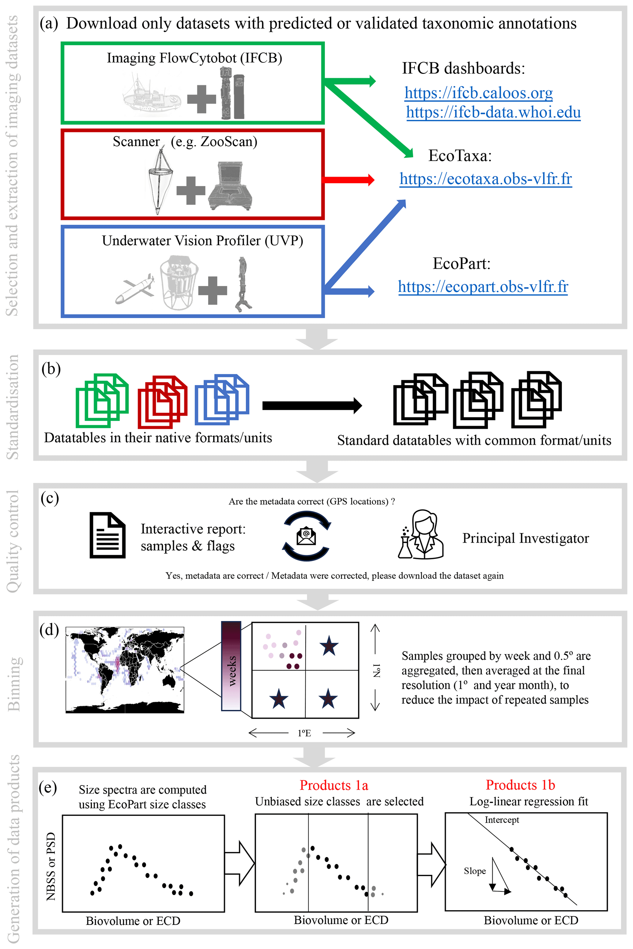
Figure 1Schematic of the PSSdb processing pipeline. The main steps of the pipeline include (a) the selection and automatic download of imaging datasets that include predicted or validated taxonomic annotations (to ensure that bulk datasets do not include artifacts and to generate taxa-specific products), (b) the standardization of their native formats and units, (c) quality controlling involving an exchange between PSSdb developers and the concerned principal investigators, (d) the binning of samples in spatio-temporal proximity to match the current resolution of other databases and biogeochemical models, and (e) the computation of size spectra and the generation of the data products released at https://dx.doi.org/10.5281/zenodo.11050013 (Dugenne et al., 2024b).
2.2.1 Selection of imaging data streams
The first objective of PSSdb is to estimate particle size spectra from plankton imaging devices following the FAIR principles. We thus relied primarily on online and accessible platforms created by the instrument developers to manage their datasets: IFCB dashboards (of generation 2 exclusively, as generation 1 does not include metadata like longitude and latitude) and EcoTaxa or EcoPart, developed for ZooScan and UVP but also for the IFCB and other imaging systems since a few IFCB datasets ingested in PSSdb were available on EcoTaxa. IFCB dashboards are deployed by individual labs or regional networks with specific URLs and are publicly accessible. Conversely, EcoTaxa datasets are not accessible by default; thus, data providers who wanted to contribute to the PSSdb were asked to provide access to their projects.
Both IFCB dashboards and EcoTaxa contain sample metadata; raw images; their related morphometric measurements; and, optionally, their taxonomic annotation. To ensure that size distributions were representative of living (i.e., planktonic and micro-nektonic organisms) and non-living particles (i.e., marine snow, fecal pellets) only, we selected datasets with predicted and/or curated image classification. This allowed for the exclusion of particles labeled as artifacts, bubbles, calibration beads, microplastics, and others. Of the 37 datasets on the IFCB dashboards and the 3290 UVP, scanner, and IFCB datasets on EcoTaxa (last checked on October 2023), only 6 projects from IFCB dashboards and 250 projects from EcoTaxa were downloaded and integrated into the first PSSdb release products. The list of the datasets (and their URLs) that are ingested in the first PSSdb release can be downloaded at https://doi.org/10.5281/zenodo.11050013 (Dugenne et al., 2024b) from the “data sources” spreadsheet included in the compressed release data files. The dataset list was generated automatically using the EcoTaxa and IFCB dashboards' application programming interface (API), which also provides fast and automatic access to both data (morphometric measurements and taxonomic annotation) and metadata.
2.2.2 Extraction of imaging data streams
All functions to list (funcs_list_projects.py) and export (funcs_export_projects.py) datasets from IFCB dashboards and EcoTaxa or EcoPart automatically are available at https://github.com/jessluo/PSSdb/tree/main/scripts (last access: April 2024). To export IFCB datasets, sample-specific queries to the IFCB dashboards are executed sequentially to retrieve sample metadata such as location, time, and depth plus the morphometric measurements of individual ROIs stored in the “features” files and the top five taxonomic predictions stored in the “autoclass” files. Metadata, feature, and autoclass files are then combined in a single master table, with a row for each ROI, and are saved into multiple files comprising ∼500 000 rows to limit the size of the exports and the processing time.
Scanner and UVP datasets were automatically exported from EcoTaxa using the API with the default option. This option retrieves all the information relative to individual ROIs (e.g., area, taxonomic annotation) and samples (e.g., location, depth, time), as well as specific acquisition (e.g., size fraction scanned and associated volume) and processing (e.g., pixel calibration factor) steps.
To further retrieve the size and count information of small particles processed by UVPs in real time, which are only uploaded to EcoPart, we wrote a custom script based on existing web-scraping python modules (function “EcoPart_export” at https://github.com/jessluo/PSSdb/tree/main/scripts/funcs_export_projects.py, last access: April 2024). We selected the “raw” export option for all datasets hosted on EcoPart rather than the default export option, which provides summary statistics consisting of the summed particle counts and biovolume in individual size bins, computed in 5 m depth bins. With the raw export option, we were able to retrieve the number of particles (column “nbr”) of a given pixel-based size measurement (column “area”), as well as the number of individual image frames (column “imgcount”, used to calculate the cumulative volume) in 1 m depth bins. This strategy has multiple advantages as it allows the conversion of pixels into metric area estimates using either the power-law function described in the Appendix A2 or a fixed pixel size. It also allows for the construction of size spectra using custom size bins and for an assessment of the uncertainty of the size spectra estimates using the bootstrap approach published by Schartau et al. (2010).
Using a pair of identifiers allowing us to link each UVP dataset uploaded on EcoPart to its corresponding EcoTaxa ID, the datasets on both platforms were consolidated into a single table to account for all particles detected by the UVP. Since EcoPart raw data files are summarized in 1 m depth bins, it is impossible to link a specific area estimate to the corresponding EcoTaxa vignette and, thus, its taxonomic annotation. To consolidate data for all particles in 1 m depth bins without losing further information and without including the same particle twice, we used the threshold for vignette generation to select particles with and without a taxonomic annotation (particles larger than ∼910 or 690 µm in equivalent circular diameter (ECD) for the UVP5 and UVP6, respectively). The consolidated UVP data files thus include the area estimates from all particles smaller than this threshold, which are assigned an empty taxonomic annotation, along with the area and taxonomic annotations of each ROI stored in EcoTaxa data files, whose sampling depth precision is reduced to the resolution of EcoPart data files (i.e., 1 m bin levels). All metadata for the sampling locations, depth range, and pixel size were merged into this unique table using the metadata file exported from EcoPart.
2.2.3 Standardization of imaging datasets
Since raw datasets exported from the API queries are generated with different formats, with specific headers and units, we developed instrument-specific “standardizer” spreadsheets in order to re-format all datasets to the same standard. Each spreadsheet contains the dataset IDs for a given instrument, including the pair of IDs required to consolidate UVP datasets (see Sect. 2.2.2) and the information required for the standardization and quality controlling of these datasets. The dataset ID lists are generated automatically, but the data information (headers and units) is manually filled to map the native headers and units of the data files to standard names (following the variablename_field nomenclature) and units (following the variablename_unit nomenclature). After listing and exporting all datasets from EcoTaxa, EcoPart, or IFCB dashboards, a member of PSSdb thus enters the name and corresponding unit found in the native export files into each variable needed in future steps of the pipeline so that they can be mapped and converted into the standards defined in the product documentation. This mapping and conversion is then done automatically using the script developed for the standardization (https://github.com/jessluo/PSSdb/blob/main/scripts/2_standardize_projects.py, last access: April 2024). The spreadsheets can be downloaded at https://github.com/jessluo/PSSdb/tree/main/raw (last access: April 2024) under project_Instrument_standardizer.xslx.
The mapped variables include longitude, latitude; sampling time (with time format); minimum and maximum sampling depth; volume sampled and potential dilution or concentration factors; the lower and upper sample size limit; and optional additional metadata describing the sampling effort, protocol or downstream processing, the pixel size, and the ROI size estimates with taxonomic annotation. In the case of size-fractionated samples, the sampling size limits were determined by the mesh or filter sizes. Otherwise, the dimensions of the imaging frame are used to specify the theoretical upper size range imaged by the device. ROI size estimates may include biovolume, area, or ellipsoidal axis for comparison. However, the size spectra for PSSdb were all computed using ROI area for consistency across devices since not all imaging instruments provide biovolume estimates and the derived equivalent spherical diameter (see Sect. 2.2.6 for more details). In addition, the value(s) for “not available” or NA were specified, if necessary, since we found some inconsistencies in the values reported, particularly for datasets generated by Zooprocess (i.e., UVP and scanner datasets), depending on the software version used, but also across variables for the same dataset. While the standardizer spreadsheet needs to be filled manually, we found this approach to be optimal to account for the variable formats of existing and future datasets, both accessible online or directly sent to us.
Native units, defined in the standardizer spreadsheets, are converted to standard units using the Python package Pint (https://pypi.org/project/Pint/, last access: October 2023), designed to define, operate, and manipulate physical quantities based on units from the International System or defined in a custom text file. Custom units defined for PSSdb included the pixels per micrometer and pixels per millimeter used to convert pixel-based size estimates to metric-based estimates (https://github.com/jessluo/PSSdb/blob/main/scripts/units_def.txt, last access: April 2024). After standardization, an interactive report is generated to check that units were correctly assigned by displaying the NBSS computed according to Sect. 2.2.6 and the average particle size and/or concentration for individual samples. PSSdb developers can then check that both the size range and the overall concentration recorded are consistent with the particle size targeted by specific instruments (Lombard et al., 2019). This step ensures that the file format and units in all data files are consistent, enabling the further merging of the data in the following PSSdb workflow steps.
2.2.4 Quality controlling of imaging datasets
After morphometric measurements, taxonomic annotations, and metadata from the imaging data streams are downloaded (see Sect. 2.2.2); the standardizer spreadsheets are filled (see Sect. 2.2.3); and all datasets are standardized, a quality control (QC) check is performed on individual IFCB, UVP, and scanner samples. The objective of this step is to ensure the good quality of the datasets ingested in PSSdb by automatically flagging individual samples whose size spectrum computation was either impossible (missing required information) or biased (incorrect GPS coordinates, pixel size, or low ROI number). We used a Boolean factor to characterize each flag, assigning 0 (false) to non-flagged samples that passed the quality control and 1 (true) to flagged samples. Currently, seven criteria are checked during the QC, and the overall flag is assigned 0 if the sum of the individual flags equals 0; otherwise, it is assigned a value of 1.
The first flagging criterion stands for missing required data or metadata, as specified in the standardizer spreadsheets. Second and third, GPS coordinates are checked to verify whether they are located on land, according to the georeferenced Global Oceans and Seas dataset (version 1 automatically downloaded from https://www.marineregions.org/, last access: October 2023), or located at 0° × 0° latitude and longitude, which sometimes indicates that this information has not been filled correctly. Fourth, to determine whether the number of ROIs (n) in a sample was sufficient to accurately estimate a size spectrum, we estimated count uncertainty assuming that particle detection followed a Poisson distribution (Schartau et al., 2010; Bisson et al., 2022; Haëntjens et al., 2022). According to this distribution, the accuracy of ROI counts decreases significantly with lower count numbers n. We could thus estimate the probability of effectively observing n ROIs given that the mean occurrence (the main parameter of the Poisson distribution) was equal to n, and we assigned a flag to samples whose ROI counts yielded more than 5 % uncertainty. Fifth, the percentage of manual taxonomic annotations (verified by a human expert) is calculated in order to flag samples that are less than 95 % validated. This criteria is only applied to scanners and UVP datasets as the larger number of IFCB images per sample makes it more difficult to manually validate automated classifications. Sixth, the percentage of artifacts per sample is evaluated using the predicted or validated annotations so that any sample with 20 % or more artifacts is flagged. Finally, samples with multiple pixel size factors are also flagged since we do not expect the camera to be re-calibrated or replaced during deployment.
After the completion of the QC, a table summarizing individual samples with their flags and an interactive report providing an overview of the samples flagged for each dataset are automatically generated. The interactive report is checked by PSSdb developers and sent to the data providers for an overview of the dataset sample locations, the number of ROIs, the percentages of validations and/or artifacts per sample, and the overall percentage of flagged samples. Hyperlinks are inserted in the interactive report to verify the sample information directly from the data source. Flags may be overruled by the data provider if they consider a sample to be suitable (or not) for incorporation into PSSdb. For example, samples that have been size-fractionated could record a low ROI number, samples with a high percentage of artifacts may not necessarily be completely biased, and low validation may be acceptable if all artifacts have been correctly identified.
2.2.5 Binning of imaging datasets
After standardization and QC, we first selected datasets where the sampling depth was between 0 and 250 m (Fig. A1). Samples were aggregated spatially in cells of 0.5° × 0.5° latitude and longitude and temporally per week. This data aggregation approach allowed us (1) to increase the overall volume analyzed per sample, which increases the number of particles observed and decreases the instrumental detection limit, and (2) to avoid the over-representation of data from fixed time series stations with high temporal sampling compared to co-located “snapshot” samples in a given grid cell. The size spectra calculations described in the next section were performed on these weekly, 0.5° × 0.5° samples. Since, unavoidably, some weeks of a year might be shared between 2 months, we assigned that week to the month that counted the most samples. This approach prevented the creation of duplicate weekly samples per year. The final data products included in the first release (1a: bulk normalized biovolume or abundance per size bin; 1b: slopes, intercepts, and determination coefficients of the size spectra) are reported as monthly, 1° × 1° grid averages, such that each mean size spectrum, slope, and intercept had a maximum sample size of 16, the product of four 0.5° × 0.5° sub-cells in a 1° × 1° cell and 4 weeks per month. As mentioned above, reporting monthly, 1° × 1° grid parameter averages from the subgrid values instead of calculating directly the size spectra for these larger bins prevents a certain location or time series with a higher number of samples from skewing the size spectra estimate, especially in a 1° × 1° cell that contains both open-ocean sites sampled during research cruise(s) and coastal time series sites.
2.2.6 Computation of bulk particle size spectra and regression parameters from binned, instrument-specific datasets
The particle size classes used in PSSdb were previously defined in Kiko et al. (2022). These are logarithmically spaced using a base of 2 and an increment of so that a doubling in equivalent circular diameter (ECD) is observed in every third bin (equivalent to a doubling in biovolume observed in every bin), with a range between 1–50 000 000 µm. The diameter of each particle, with the exception of artifacts which are excluded from the size spectra computation, was estimated using area according to Eq. (1) and then was converted into biovolume assuming a spherical shape of that diameter following Eq. (2).
Area-based biovolume, rather than the more widely used distance map estimates for IFCB datasets (Moberg and Sosik, 2012), and ellipsoidal fits for scanners and UVP datasets (Dubois et al., 2022) were selected to keep the size spectra calculations consistent across instruments. However, a sensitivity analysis of the slopes and intercepts as a function of the different size proxies (ellipsoidal, distance map, and area-based biovolume) is presented in Fig. A2. Despite some differences in size spectra thresholding, likely due to elongated particles being assigned to different size classes (Fig. A2a, b and c), our sensitivity analysis does not show any substantial differences between size spectra parameters from different biovolume estimates (Fig. A2d, e and f). This aligns with previous comparisons of elliptical or spherical biovolume-derived size spectra, which found no or little statistical difference between these estimates (Vandromme et al., 2012; Dubois et al., 2022).
The database includes size spectra calculated by two widely used methods: the normalized biovolume size spectrum (NBSS), routinely reported in zooplankton studies (e.g., Zhang et al., 2019; Grandrémy et al., 2023c), and the particle size distribution (PSD), calculated from particle counters (broadly) (Kiko et al., 2022) or derived from satellite algorithms (Kostadinov et al., 2009). For NBSS, the normalized biovolume (NB) () for each biovolume size class (i) in a sample (0.5° × 0.5° grid cell, grouped by week) was calculated as the summed biovolume (µm3), normalized by the cumulative volume sampled (L) and the biovolume bin width (µm3), as in Eq. (3):
For PSD, the normalized abundance (NA) (number of particles L−1 µm−1) for each size class (i) in a sample was calculated as the total number of particles in ECD size class i, normalized by the cumulative volume sampled (L) and the ECD bin width (µm), as in Eq. (4):
Retrieved size spectra were generally biased at the lower and upper size limits (Fig. 1e). At the lower end, the main bias is due to the sampling collection method (e.g., mesh of the net) or the segmentation threshold (e.g., minimum area or mean gray level), which randomly excludes small particles, such that the closer the particles are to the camera resolution, the less likely they are to be imaged and segmented. At the higher end, imaging systems overestimate larger, rarer particles whose concentrations are close to the instrument detection limit, as determined by the imaging volume. As a result, size spectra would typically display an inflection point at the lower size limit and remain quasi-constant (e.g., flatter) at the upper size limit. The unbiased portion of the size spectrum was identified before computing the size spectra slopes and intercepts by log-linear regression. To do so, we first exclude data from size classes with either a size measurement or particle count uncertainty greater than 20 % assuming Gaussian and Poisson error distributions, respectively. These distributions are based on the statistical analysis developed by Schartau et al. (2010) to quantify the size spectrum uncertainties, which assumes that size measurement uncertainties follow a Gaussian distribution with a variance equal to the camera resolution and that the uncertainty of effectively observing ROIs given a similar occurrence of particles within the volume sampled follows a Poisson distribution. According to this distribution, counting four or fewer ROIs in each size bin would yield an uncertainty greater than 20 %. We thus reset the normalized biovolume or abundance of size classes with four or fewer ROIs – mainly larger size classes – as empty size classes and selected the upper size limit as the largest size class before observing three consecutive empty size classes. Our choice for the upper size limit definition was a compromise between unnecessarily excluding large organisms and including too many large bin values that would bias the size spectra calculation towards flatter slopes. Next, we selected the size bin of the maximum normalized biovolume or abundance value as the lower size limit. It is important to clarify that this thresholding is applied to the weekly, 0.5° × 0.5° bins; thus, it is possible that 1a products present low normalized or abundance values at the lower end if the smallest size class is present in only some sub-bins. After selection, size spectra followed a power-law function in the form of Eq. (5), with a log-transformation resulting in a linear equation of the form described in Eq. (6):
The slope (b, L−1 µm−3 for NBSS and L−1 µm−2 for PSD), intercept (I, for NBSS and # L−1 µm−1 for PSD), and coefficient of determination (R2) of the size spectra were computed by log-linear regression following Eq. (6). An easy way to interpret the intercept values is that they refer to the normalized biovolume and abundance predicted for standard 1 µm3 and 1 µm particles, respectively.
All products (1a: size spectra, 1b: regression parameters) generated are subjected to an additional QC to provide a flag (0 if a spatio-temporal bin passed the QC, 1 otherwise) that can help data users filter out questionable data. The current QC is based on three criteria, whereby a positive flag is assigned to (1) slope values exceeding the mean ±3 standard deviations of each instrument-specific product, (2) a spectrum that only record four or fewer non-empty size classes, and (3) a log-linear fit whose regression fit R2≤0.8.
3.1 Spatio-temporal coverage of imaging datasets
Up to 92 472 individual samples are included in the first release of PSSdb, which benefited from long-term IFCB time series collected at a 20 min frequency (Table 1). In comparison, the UVP and scanner datasets comprise fewer profiles and nets, with a total of 3068 profiles and 2411 net samples, respectively.
Table 1Spatio-temporal range of instrument-specific datasets included in the first release of PSSdb.
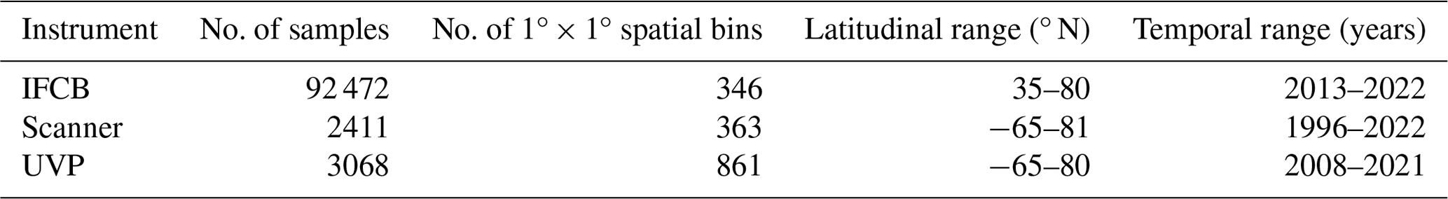
These datasets span most major ocean basins, although all basins are undersampled in the Southern Hemisphere. IFCB datasets that have been ingested in our database were all restricted to the middle to high latitudes of the Northern Hemisphere (Fig. 2, Table 1). Further, the majority of IFCB samples are located on the shelf of the eastern and western United States due to the presence of long-term time series sites of the California Ocean Observing System and the Northeast US Shelf Long-Term Ecological Research programs (Fig. 2a). UVP and scanner datasets are distributed more evenly across the ocean basins, mostly due to the Tara Ocean (2009–2012) and Tara Polar Circle (2013) global expeditions, even though specific monitoring programs increased the density of samples in the tropical Atlantic, the eastern temperate Atlantic, and the Mediterranean Sea (Fig. 2b, c). These monitoring programs resulted in a large temporal coverage of the three instrument-specific datasets, with repeated observations sustained for periods of 10–25 years (Fig. 2d, e, f; Table 1). Notably, the scanners show the largest temporal coverage, from 1996 to 2022, by including samples collected at the long-term monitoring sites located in the Bay of Villefranche-sur-Mer and the Bay of Biscay (France). The gap observed between 1998 and 2003 is caused by the exclusion of samples that had not been validated to at least 95 %. This high-frequency dataset affected the monthly variability of the scanners' sample density, shown in Fig. 2e, since the Bay of Biscay monitoring program only takes place in May (Grandrémy et al., 2023a). UVP datasets have the second longest coverage, with observations collected between 2008–2021 (Fig. 2f). In PSSdb's first release, the climatology of UVP sampling density is slightly biased towards spring months (March, April, and May); however, this may not reflect actual sampling efforts as UVP images also need to be more than 95 % validated to be ingested in PSSdb. This threshold is not applied to IFCB datasets, which comprise too many images to be manually curated, yet the datasets also show a strong bias towards the summer months (June, July, August). This bias reflects the sampling strategy of both the NESLTER broad-scale program, limited to the summer months, and the CalOOS sampling program, both of which partially operate with IFCBs serviced during the wintertime to avoid damage. IFCB has been routinely deployed at the Martha's Vineyard Coastal Observatory since 2006; however, only samples from 2013 and after were included in PSSdb as previous observations did not include taxonomic predictions, which were required to filter artifacts out of the data products (Table 1; Fig. 2d).
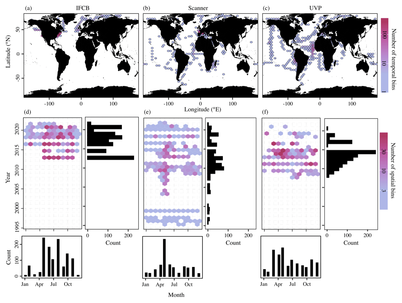
Figure 2Spatio-temporal coverage of PSSdb first-release datasets obtained from the IFCB (a, d), scanners (b, e), and the UVP (c, f). Maps and Hovmöller diagrams are color-coded according to the density of temporal bins (a–c), corresponding to the year and month, and spatial bins (d–f), corresponding to 1° × 1° grid cells, respectively. The sizes of the grid cells are expanded () in panels (a), (b), and (c) to help visualize the color scale and represent a coarser spatial coverage of the dataset.
3.2 Size spectra obtained from individual imaging devices
The IFCB effectively detects and images plankton and detrital particles in the nano and micro size fractions. This size range is supplemented by UVP and scanner datasets, which include predominantly living microplankton and mesoplankton (Table 2). We used two metrics to evaluate pelagic size structure from plankton imaging devices: the NBSS, computed with normalized biovolume (Eq. 3), and the PSD, computed with normalized abundance (Eq. 4). Both metrics showed similar patterns, resulting in high correlations between the fitted parameters, namely the NBSS and PSD slopes (r=0.99), intercepts (r=0.99), and determination coefficient R2 (r=0.99) (Fig. 3). For simplicity, we further describe observed patterns of the instrument-specific size spectra parameters derived from NBSS only since both PSD and NBSS co-vary. However, all patterns and trends described in the following sections, including in the discussion, hold for the PSD releases.
Global size spectra slopes and intercepts were relatively consistent between instruments, with average values of ∼ −1 L−1 µm−3 and ∼107.6 µm3 L−1 µm−3 (corresponding to an approximate concentration of 4×107 µm3 L−1 µm−3 for particles of 1 µm3), respectively (Table 2, Fig. 3). The UVP's size spectra presented an intercept slightly above that of the IFCB and scanners, given the additional particles they can detect in situ, with overall higher R2 estimates, although relatively large R2 values were observed across all instruments (Table 2, Fig. 3).
Table 2Size spectra description for each instrument included in the first release of PSSdb. Parameters are reported as mean (± standard deviation), with the exception of the untranslated intercept, which is reported as a geometric mean, with the range of observed values given as the first and third quartiles in the parentheses.
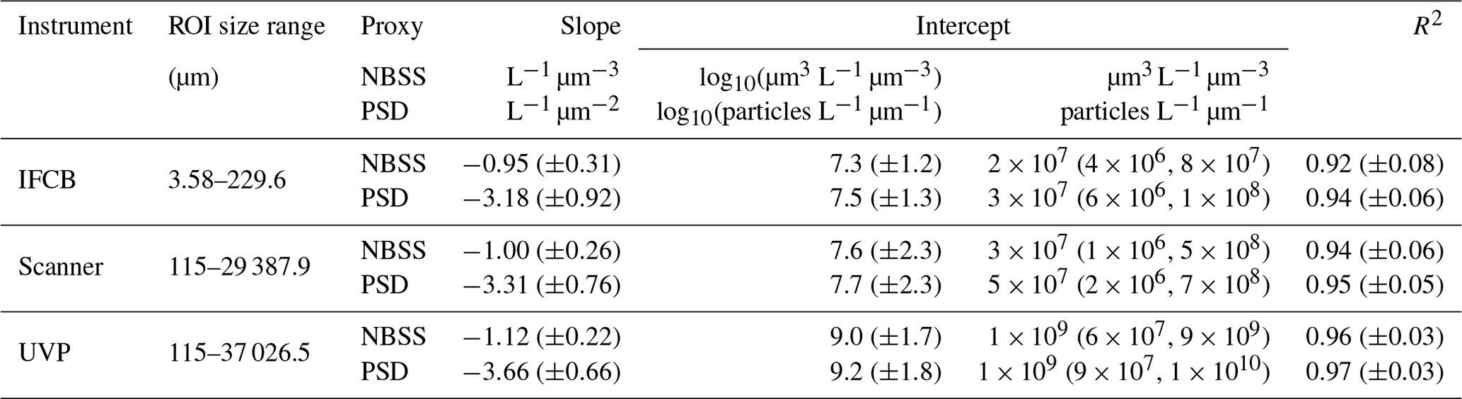
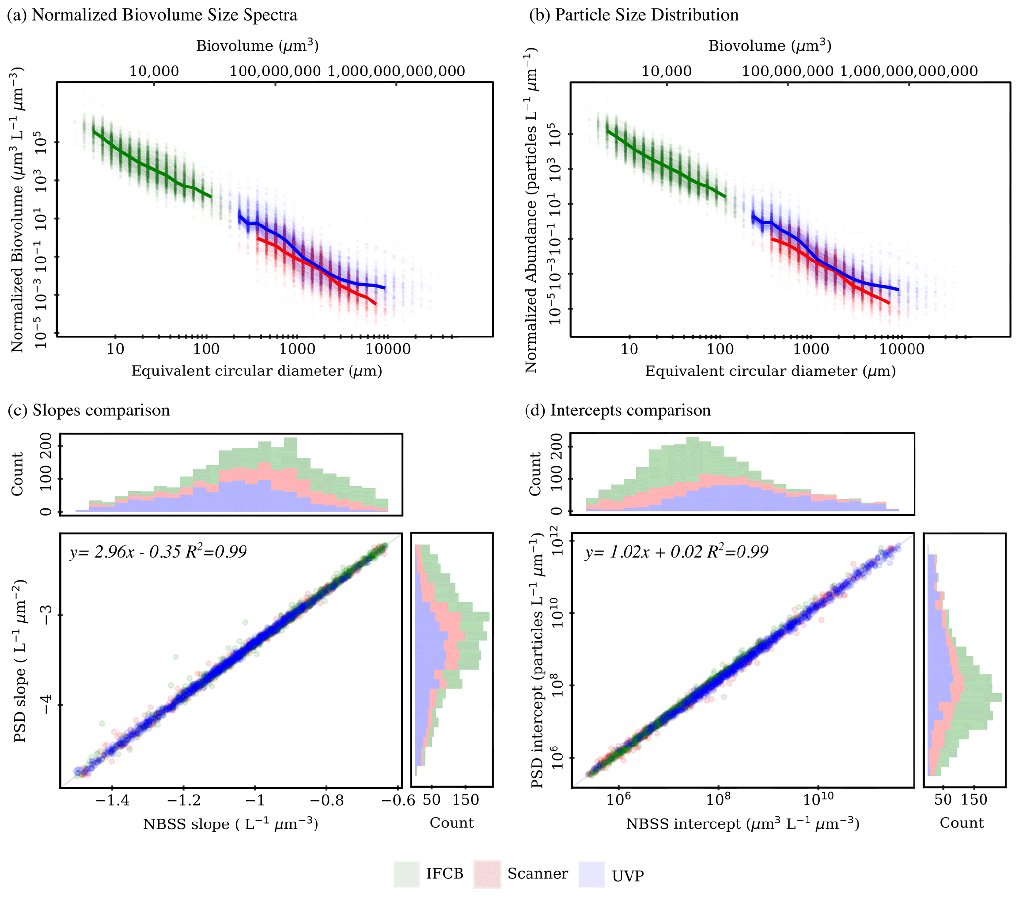
Figure 3First release of PSSdb: pelagic size spectra (product 1a) approximated from normalized biovolume (a) and normalized abundance (b) and comparison between fitted (products 1b) slopes (c) and intercepts (d) for the three plankton imaging systems included in the first release. Solid lines in panels (a) and (b) represent the median spectrum, restricted to size classes that were observed in at least 50 % of the samples to avoid misalignment due to different sampling efforts (e.g., different mesh sizes for scanners, different photo-multiplier (PMT) settings for IFCB).
3.3 Size spectra regression fit, slopes, and intercepts
In addition to the average, instrument-specific differences reported above, PSSdb allows for an exploration of the spatial and temporal variations in the NBSS and PSD (not shown since they co-vary with NBSS) for individual instruments. Figure 4 shows the average NBSS slopes, intercepts, and R2 values obtained for each grid cell in the global ocean. Despite their similar size targets, there were substantial differences in the global distribution of NBSS slopes and intercepts derived from the three imaging approaches. Indeed, while the majority of the slopes were around −1 L−1 µm−3, the scanner slopes showed no clear variation with space. Meanwhile, the UVP slopes tended to show steeper size spectra within oligotrophic gyres and flatter size spectra in the northernmost latitudes or by the coasts (Fig. 4c). This pattern was inverted with regards to the intercepts as the abundance of 1 µm3 particles was lower in the Arctic and increased near the shore (Fig. 4f). Likewise, the IFCB NBSS slopes were indicative of flatter size spectra, with lower intercepts, in the northernmost latitudes and along the eastern coast of the United States compared to the western coast (Fig. 4a, d). The determination coefficients seemed to follow an inverse relationship with the slope for the IFCB NBSS as flatter NBSSs were also marked by lower R2 (Fig. 4g). The scanner data did not follow such clear trends and seemed less variable than the UVP and IFCB (Fig. 4b, e), although there seemed to be a clear decrease in NBSS linearity, or R2, towards the pole (Fig. 4h).
To check whether these trends were specifically linked to sampled latitude, we looked at the latitudinal variability of the NBSS parameters (Fig. 5). IFCB measurements were all restricted to a small latitudinal range; however, we observed a notable decrease in the linearity of the size spectra with latitude. Higher latitudes (>50° N and S) also showed higher variation in both slope and intercept estimates compared to lower latitudes, as well as lower coefficients of determination for scanner and UVP size spectra. Both show a reduced variability in derived slopes and intercepts within the tropics, with flatter slopes and increased intercepts notably being located at 0° N, near the equatorial current system. Since latitudinal trends can be impacted by different dynamics in specific regions but also by differences across seasons, we computed the instrument-specific monthly climatologies of NBSS parameters in ocean regions where there were at least 10 months of data (Fig. 6). This excludes the Arctic Ocean, Red Sea, South Atlantic, Southern Ocean, and Baltic Sea, which are represented in PSSdb but do not have enough data to resolve seasonal cycles.
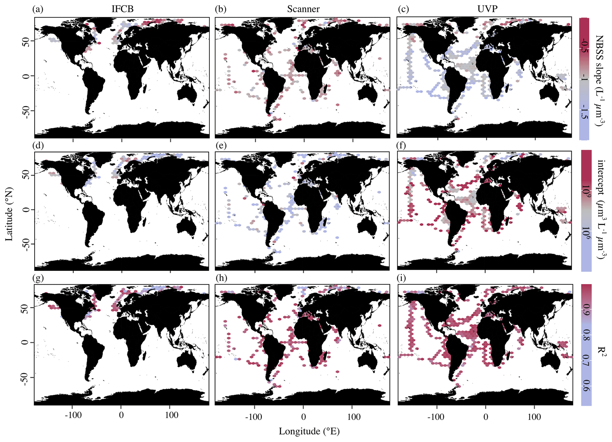
Figure 4Average NBSS parameters in 1° × 1° latitude–longitude cells (product 1b) from imaging data obtained by the IFCB (a, d, g), scanners (b, e, h), and the UVP (c, f, i). Slopes correspond to panels (a), (b), and (c); intercepts correspond to panels (d), (e), and (f); and determination coefficients correspond to panels (g), (h), and (i). The sizes of the grid cells are expanded () in all panels to help visualize the color scale and represent a coarser spatial coverage of the dataset.
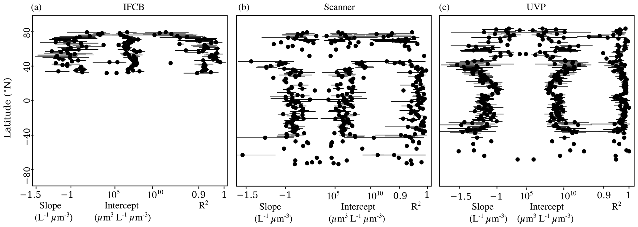
Figure 5Latitudinal variability of NBSS slopes, intercepts, and determination coefficients for the IFCB (a), scanners (b), and the UVP (c). Dots represent the mean parameter value per 1° latitudinal bins, and the horizontal bars represent the standard deviation.
Time series analysis of the instrument-specific NBSS showed pronounced seasonal cycles but high variability by region and, in some cases, between instruments. Seasonal variations in NBSS parameters were apparent for most ocean basins, as well as in the Mediterranean Sea (Romagnan, 2013), which showed high variation in terms of the scanner mean slope and intercept throughout the year (Fig. 6b,g), with rather constant R2 values (Fig. 6l). Stable R2 values were generally observed across all instruments and ocean basins, with the exception of the scanner datasets located in the Indian Ocean, which presented a large dip in NBSS linearity in October (Fig. 6k). Interestingly, the North Atlantic presented opposite trends between the IFCB and the scanner, whose NBSS slopes indicated a steepening of the size spectra and whose intercepts increased during the spring (Fig. 6c, h), and the UVP datasets, for which the NBSS flattened and intercepts decreased during spring and summer (Fig. 6c, h). In the Southern Hemisphere, UVP slopes were at a minimum by the end of austral summer (January–May), with a concurrent increase in NBSS intercepts only observed by the end of this period (Fig. 6e,j). Scanner datasets showed similar trends to those of the UVP in the South Pacific, except that the minimum slope and maximum intercept were observed by March, earlier in the year. The Indian Ocean followed the same seasonal cycle, with large differences between seasons as spectra steepened and intercepts increased during the spring–summer transition while remaining relatively stable at high slope and low intercept values from September through November (Fig. 6a, f). Lastly, the IFCB datasets collected in the North Pacific presented two peaks in NBSS intercepts, with concurrent dips in the slopes, indicative of a steeper NBSS, by spring (April) and fall (Oct) (Fig. 6d, i).
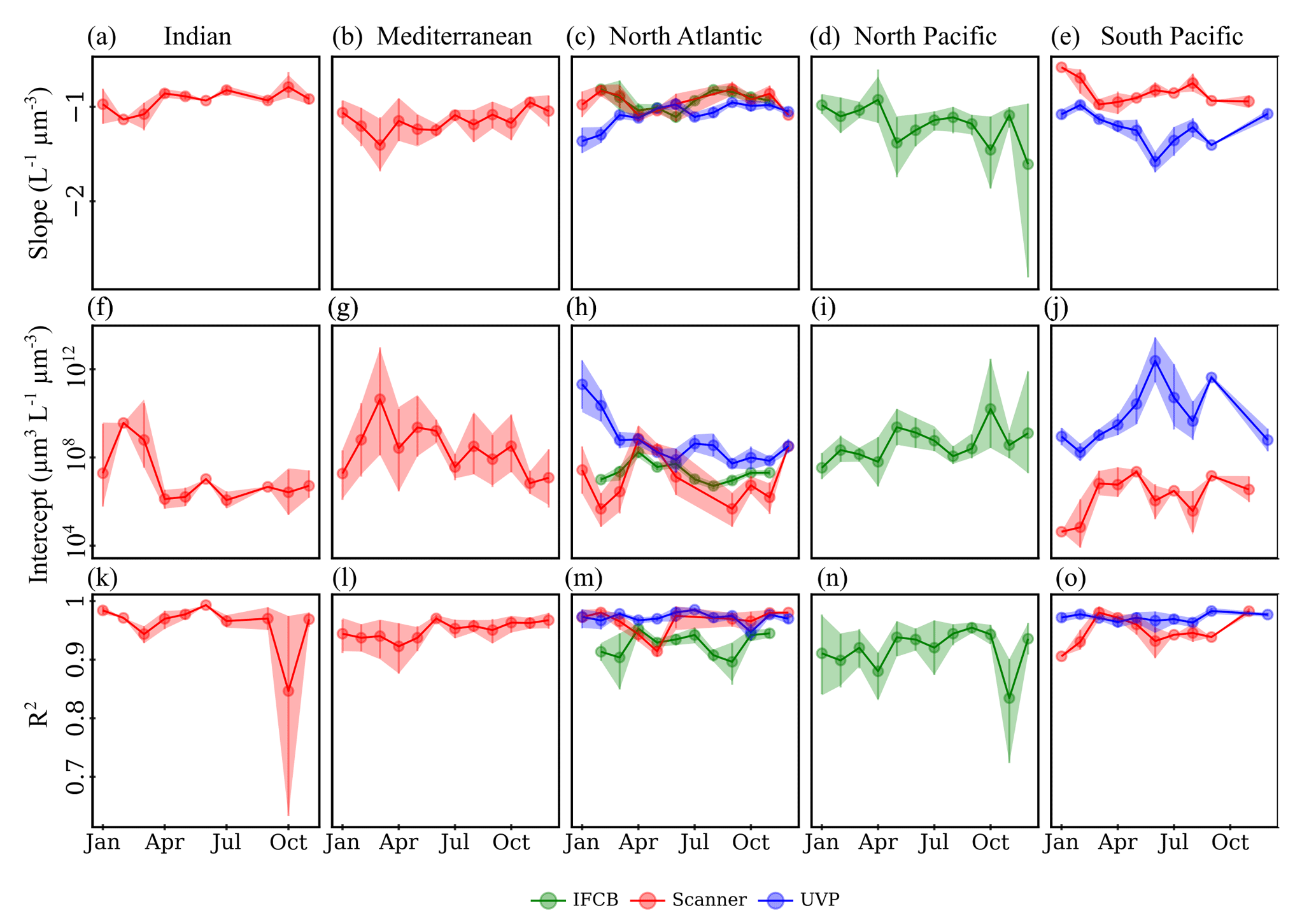
Figure 6Climatologies of NBSS slopes (a–e), intercepts (f–j), and R2 (k–o) for each imaging system. The data are shown for five major ocean basins, with enough data to show seasonal fluctuations: Indian Ocean (a, f, k), Mediterranean Sea (b, g, l), North Atlantic (c, h, m), North Pacific (d, i, n), and South Pacific (e, j, o). Vertical lines represent the standard deviation of the monthly average parameters.
Given the opposite spatial (Figs. 4, 5) and temporal (Fig. 6) patterns typically observed between the size spectra slopes and intercepts (Sprules and Barth, 2016) across instruments and oceanic regions, we used the yearly time series correlation of these two parameters in any given grid cell within the same oceanic region as a way to detect potential decoupling, lag, or feedback between the two. The (de-)coupling between NBSS slopes, which represent the balance between relatively small and large particles and plankton, and intercepts, which approximate the carrying capacity of a given ecosystem, across the years is presented in Fig. 7. As expected, the majority of PSSdb grid cells were strongly anti-correlated, with coefficients close to −1, since steeper size spectra tend to indicate an increased proportion of smaller particles, which are generally more abundant. Noticeably, though, there are also areas of a strong positive relationship between the two parameters, especially within the IFCB datasets located in the North Atlantic. Flatter NBSS values were thus associated with increased abundances of 1 µm3 organisms, which could be indicative of the relief of nutrient stress, allowing for multiple phytoplankton size groups to co-exist (Armstrong and McGehee, 1980); other complex interactions between primary producers dictated by resource competition; or trophic shunt between small and large plankton for zooplankton. In this region, we also observed a de-coupling between the NBSS parameters for 2–3 years, as indicated by grid cells with low absolute correlation coefficients. A de-coupling between size spectra parameters could arise from temporal lag in trophic transfer and complex trophic cascading, similarly to that mentioned above. Care should be taken when testing for significant long-term trends in the coupling of the NBSS parameters and when detecting yearly perturbations; however, we expect such analyses to become more robust as more datasets are ingested into the future releases of PSSdb.
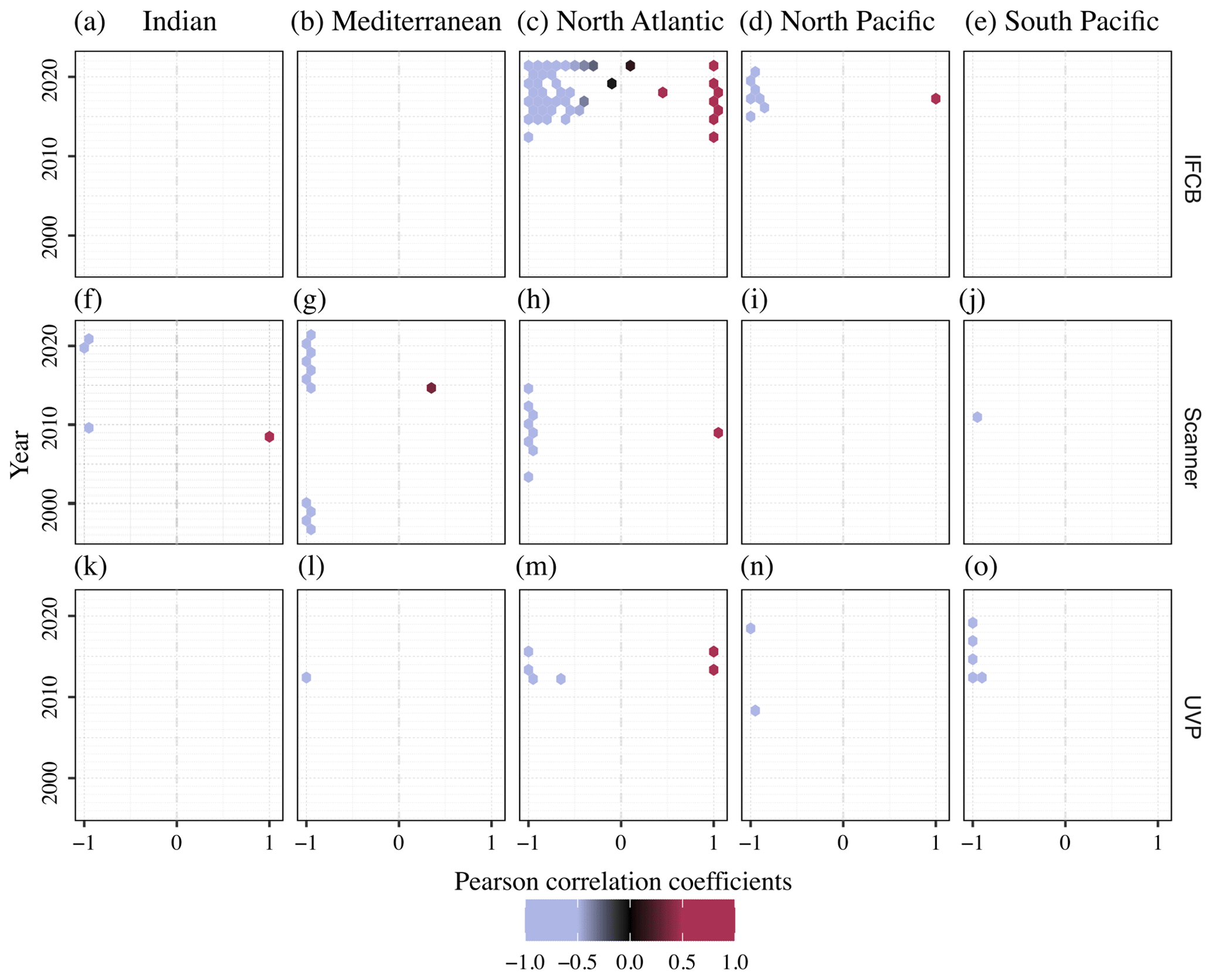
Figure 7Pearson correlation coefficients between NBSS slopes and intercepts across ocean basins (columns) and years for the IFCB (a–e), scanners (f–j), and the UVP (k–o). Each data point represents an individual grid cell within the five major ocean basins, with enough data to show seasonal fluctuations: Indian Ocean (a, f, k), Mediterranean Sea (b, g, l), North Atlantic (c, h, m), North Pacific (d, i, n), and South Pacific (e, j, o).
Workflows that provide estimates of plankton size distributions with an extensive spatial and temporal coverage will greatly accelerate efforts to characterize and understand ecological plankton dynamics at a global scale. With this goal, the first PSSdb data products were generated to determine patterns in trophic transfer efficiency across plankton sizes and ecosystem carrying capacity through consistent measurements of particle sizes analyzed by three state-of-the-art plankton imaging devices. In this section, we discuss how the spatial and temporal coverage of these instrument-specific datasets effectively reduce the gap in available size structure observations before presenting potential uses of the datasets and future directions for the database.
4.1 The contribution of PSSdb and other data compilations to reducing the gap in available size structure estimates
A global compilation of particle size distribution has recently been published by Kiko et al. (2022) using the UVP5 bulk particle size distribution accessible from EcoPart. Other recent studies (e.g., Hatton et al., 2021) have also constructed global estimates of size distribution in marine organisms using indirect biomass estimates of arbitrary plankton size classes derived from satellite proxies, models, or data compilations like COPEPOD (Moriarty and O'Brien, 2013) and the MARine Ecosystem biomass DATa (MAREDAT, Buitenhuis et al., 2013) without relying on direct size estimates. More recently, Atkinson et al. (2024) compiled estimates of spectral slopes measured in 41 sites, mostly located in the Atlantic Ocean and a number of lakes, displaying important characteristics relevant to studying the impact of climate change. Such databases and compilation efforts have benefited from exponentially growing sampling efforts during the past decades, with hundreds to thousands of new UVP profiles generated each year (Kiko et al., 2022). Yet, to our knowledge, our workflow is the first attempt to compile the counts, size measurements, and taxonomic information of individual particles from multiple imaging devices to generate global particle and planktonic size spectra datasets, which are intended to be accessible to the broad scientific community. Similarly to the COPEPOD database, we have focused our effort on compiling data from different instruments, sampling regimes, and data collection methodologies in a self-consistent and cross-calibrated manner, enabling ease of comparison between all the major ocean basins and across sampling systems.
So far, size spectrum studies have been restricted to accessible areas and clement weather conditions (Hatton et al., 2021), leading to fewer sampling efforts at high latitudes, specifically in the Southern Ocean and the South Pacific Ocean. Similarly, the sampling density is skewed towards the continental shelves as opposed to open-ocean stations. Like other global compilations, our datasets of marine pelagic size structure highlight multiple undersampled regions by means of plankton imaging systems. All imaging sensors were mostly deployed in the Northern Hemisphere in contrast to the fewer deployments in the South Pacific, the western Indian Ocean, and the Southern Ocean. While the latter is covered in the UVP-based compilation of particle size structure (Kiko et al., 2022), the absence of the Southern Ocean in our database results from the need for the manual validation of taxonomic annotations to pass our current quality controlling. However, as more autonomous vehicles will be equipped with UVP6 and its embedded classifier (Ricour, 2023), notably in the Bio-Argo program (Claustre et al., 2020), we anticipate that UVP6-derived datasets will grow substantially in the upcoming decade. To accommodate the growth of datasets derived from large-scale surveys, we could relax such criteria to generate specific data products in near-real time. Since a few UVP6 datasets are already incorporated in this initial release, we expect further ingestion of additional UVP6 data to be relatively straightforward.
Unlike the UVP datasets, the IFCB and scanner datasets are more difficult to compile due to the lack of a common platform to manage incoming datasets and due to the increased efforts needed during the sampling (e.g., net deployments and recoveries), pre-processing (e.g., concentration or size fractionation of particles before imaging), and post-processing steps. Notably, the large number of images collected at an hourly or sub-hourly frequency by the IFCB devices and their classification constitute a veritable bottleneck in producing near-real-time datasets. To generate smaller, more manageable datasets, user-specific settings that trigger the image acquisition based on a specific size or fluorescence value may help reduce the total number of images to be classified and the presence of smaller cells (4–7 µm) that are harder to identify, even manually. Alternatively, newer, more efficient, automated classifiers can also help manage upcoming observations (Kraft et al., 2022).
4.2 Global patterns and trends in plankton size spectrum: insights from the PSSdb first release and potential future uses
Parameters derived from the plankton and particle size spectrum (slope, intercept, and determination coefficients) are all important indicators of ecological processes (Sprules and Munawar, 1986; Trudnowska et al., 2021). As such, they can inform us about the general functioning and state of pelagic ecosystems and the eventual perturbations or shifts in plankton community structure.
The compilations from Hatton et al. (2021), Atkinson et al. (2024), and Kiko et al. (2022) seem to support the presence of an equal stock of living biomass across increasing size classes (slope of the biomass spectrum is equal to ∼0), driven by the log-linear decline in particle abundance with increasing size and/or biomass (slopes of the normalized biovolume and abundance spectrum are equal to and −4, respectively), as postulated by Sheldon et al. (1972). Small differences across instruments can be attributed to certain plankton groups being measured with more accuracy by one instrument. For instance, the UVP additionally samples fragile organisms and non-living particles, which are disrupted by the net collection (e.g., Biard et al., 2016; Soviadan et al., 2023). As a result, the UVP-specific spectra were consistently higher than the scanner spectra. Like these studies, the majority of PSSdb NBSS slopes are relatively close to −1 (equivalent of −4 for PSD), indicating a stable equilibrium between small and large particles and a similar trophic transfer efficiency (Fig. 4, Table 2). Nevertheless, substantial divergences from the canonical slope were observed for all the instruments used in this release, notably in the northernmost latitudes and close to the coasts. Size spectra have been shown to flatten with increasing nutrient supply (e.g., upwelling, coastal, and polar systems), as observed by other data compilations (see Atkinson et al., 2021, for freshwater ecosystems), modeled by size-structured plankton systems (Barton et al., 2013; Hatton et al., 2021; Serra-Pompei et al., 2022), or approximated from satellite data (Kostadinov et al., 2009; Hirata et al., 2011; Roy et al., 2013). Interestingly, we did not observe flatter size spectra in stable upwelling ecosystems located along the Californian, Peruvian, Namibian, and northwestern African coasts (Fig. 4). The shallowing of size spectra slopes with increasing nutrient supply is not a universal pattern since flatter size spectra have also been reported in stable, oligotrophic ecosystems compared to in more productive ecosystems (Marcolin et al., 2013; Atkinson et al., 2021). The former are typically considered to be at steady state, as reflected in the stable daily oscillations of total particulate organic carbon, yet significant variability in time and space raises substantial concerns regarding our ability to extrapolate plankton size spectra and their slopes from crude or fragmented observations (Rodriguez and Mullin, 1986).
A simple explanation for this lack of consistency is that all spatial patterns are effectively impacted by sampling time. Notably, our extended temporal coverage in the Indian, Pacific, and Atlantic Oceans, as well as in the Mediterranean Sea, has highlighted that there is significant variability in size spectra slopes and intercepts from month to month (Fig. 6). Most temperate regions presented a trend consistent with the formation of a spring bloom, indicated by a flattening of the size spectra, and its progression towards a more stratified environment, marked by steeper size spectra due to the predominance of smaller plankton; this is in agreement with other regional and global studies (Clements et al., 2022; Haëntjens et al., 2022). However, coastal regions sampled by the IFCB showed an opposite progression, with steeper size spectra during the spring and fall seasons, which is consistent with a shift of the phytoplankton community towards smaller dinoflagellates compared to larger diatom chains, as described in Fischer et al. (2020). Seasonal plankton dynamics in coastal systems are much harder to predict given the large number of variables that determine plankton blooms. Due to this, high-frequency monitoring with imaging systems like the IFCB can quickly detect changes in size spectra and related slope and intercept anomalies indicating shifts in the plankton community, such as the occurrence of harmful algal blooms, which represent an important threat to human health around the globe (Glibert, 2020). Temporal variations in the coefficient of determination might also be relevant in detecting community shifts. For instance, the appearance of small dinoflagellates (Fischer et al., 2020) was also linked to a lower coefficient of determination. This parameter decreases with the non-linearity of particle size spectra, and, as such, can be an important indicator of ecosystem perturbations and non-steady-state conditions.
Most studies assessing marine plankton size structure have focused largely on analyzing the slope and, to a lesser extent, the intercept of pelagic size spectra, with much less interest given to the coefficient of determination (R2). However, differences in size spectrum linearity can arise from abiotic or biotic perturbations, leading to local peak(s) of intermediate-sized organisms (Moscoso et al., 2022). “Bumps” in the plankton size spectrum have been reported or modeled under harmful algal blooms (Harred and Campbell, 2014) and transient trophic interactions (Schartau et al., 2010; Banas, 2011; Rossberg et al., 2019) and as the result of mesoscale circulation (Noyon et al., 2022) or the omission of specific groups in the observed size range (e.g., heterotrophic nanoflagellates not detected by most imaging flow cytometers targeting fluorescing organisms; see Chisholm, 1992). Non-steady-state conditions are increasingly observed, particularly in nutrient-rich systems (Cavender-Bares et al., 2001), and represent a considerable topic of interest for environmental policies. For this reason, we carefully assessed and reported size spectra non-linearity in our database, along with the other, widely analyzed parameters. Our first-release products show that regions with lower R2 were mostly located towards the North Pole and were linked, in particular, to flatter size spectra in these regions (Figs. 4, 5). Like a lower R2, a decoupling between size spectra parameters is also indicative of important perturbations or, inversely, of the resilience of a given ecosystem as a result of complex trophic interactions (e.g., temporal lag, resource competition, grazing cascades). We suggest following the yearly correlation between slopes and intercepts, as presented in Fig. 7, to detect potential deviation from the expected seasonal trends, showing anti-correlation between size spectrum slopes and intercepts (Fig. 6). More data will greatly improve the accuracy of such an analysis and will potentially help inform policy stakeholders by revealing significant, climate-driven trends in size spectra decoupling.
A more detailed interpretation of our observed patterns and trends is out of the scope of this paper. However, we hope PSSdb will be further exploited by individual research groups or stakeholders to contextualize their studies or policies. In addition, current modeled (Serra-Pompei et al., 2022) and satellite-derived (Hirata et al., 2011; Roy et al., 2013; Kostadinov et al., 2023) plankton size distributions have yet to be compared to extensive size structure observations. PSSdb could represent a potential avenue to assess the performance of models and satellite proxies, especially as new and future model outputs (Negrete-García et al., 2022) and satellite datasets (e.g., NASA “Plankton, Aerosol, Cloud, ocean Ecosystem” mission) will provide biomass measurements for an ever increasing number of plankton functional groups. Such validation is key to constraining some of their uncertainties and to gaining a mechanistic understanding of how physiological and ecological processes structure current and future marine ecosystems (Menden-Deuer et al., 2021). In addition, PSSdb users could investigate important factors driving the observed spatial patterns and temporal trends of plankton size spectra. PSSdb products could thus improve our understanding of the temporal and spatial variability of particle size spectra in specific regions, as well as provide a broader context to case studies, as showcased in Figs. 4 to 7, and support global data-driven interpolation, similarly to Hatton et al. (2021) or Clements et al. (2022).
4.3 PSSdb successes, challenges, and further considerations to maintain and expand the database
In our effort to access and compile imaging datasets from multiple devices, we found the open-source platforms (and associated APIs) developed for the IFCB, UVP, and scanner users to manage their incoming datasets to be instrumental. For example, the online dashboards are a useful tool for the IFCB data generators to assess image quality during and following deployment by quickly checking the raw images and monitoring the number of ROIs per sample and can be used to alert potential stakeholders when a species of interest is detected. However, the possibility of linking a set of metadata and a tag (e.g., in the case of suspicion of any bias) for each sample was only added recently to second-generation dashboards. As a result, a significant number of datasets accessible from first-generation IFCB dashboards were not ingested in this initial release. It is difficult to assess how many IFCB samples were not ingested due to such a lack of metadata as an exhaustive list of IFCB dashboards, which would enable better data traceability, is still missing. Similarly, a portion of scanner and other net-collected imaging datasets is not easily traceable or usable for PSSdb as some data collectors still use early tools (Zooprocess and PlanktonIdentifier, the latter of which is no longer supported) to manage their datasets. Even though our pipeline is able to ingest datasets directly sent to us, these datasets eventually become harder to trace and compile compared to the UVP datasets, which are, to our knowledge, all uploaded on EcoTaxa and EcoPart. Both web platforms offer secure, easy, and reproducible access to numerous datasets, and EcoTaxa provides access to image annotations, a key feature to follow the status of the UVP and scanner datasets that should be validated to at least 95 % to be ingested in PSSdb.
These open-source management platforms have been available to the scientific community for a decade but still suffer from a general lack of funding to support their development and maintenance. This is in contrast to the increasing funding to develop new imaging prototypes and commercial instruments (Lombard et al., 2019; Martin-Cabrera et al., 2022). Examples of imaging instruments that were not ingested in the PSSdb initial release include the Planktoscope (Pollina et al., 2022), the CytoSense (Dubelaar and Gerritzen, 2000), the FlowCam (Sieracki et al., 1998), the ZooGlider (Ohman et al., 2019), the ISIIS (Cowen and Guigand, 2008), the CPICS (Gallager, 2016), the VPR (Davis et al., 2005), and the LOKI (Schulz et al., 2010). From their associated publications, it is unclear how these datasets are archived in long-term repositories, although a few datasets collected with Planktoscope, ZooCAM, CytoSense, and FlowCam instruments have already been uploaded on EcoTaxa. Ingesting such datasets in the PSSdb database would be extremely valuable to assess extended plankton size spectra in the millimeter–centimeter size range and to bridge some of the gaps introduced by specific instrument operational ranges while providing overlapping size bins (Haëntjens et al., 2022). The latter are key for pooling datasets obtained from multiple imaging devices deployed in spatial and temporal proximity. In some cases, merging imaging datasets integrated over specific depth layers (e.g., net-collected datasets) with profiling or towed datasets is facilitated by simply integrating observations using the lowest sampling resolution (Soviadan et al., 2023); however, merging discrete (e.g., surface only) and integrated observations is more problematic without a good understanding of how the discrete measurements might change with depth. Despite such challenges, the relatively small differences between the overall intercepts and slopes of the PSSdb first-release products are greatly encouraging (Table 2). Prior to PSSdb, efforts to set guidelines and best practices for obtaining plankton observations with imaging instruments (see Lombard et al., 2019; Neeley et al., 2021) had yet to establish protocols for harmonizing these datasets across platforms given the large variability between sampling strategies, instrument detection limits, size estimates, organisms targeted, and classification schemes. We hope to build upon this first data release and recent work from Soviadan et al. (2023) to provide merged data products that will effectively span the 5 orders of magnitude that can be captured by commercially available plankton imagers (Lombard et al., 2019).
Further, we planned to release taxonomically resolved PSSdb products, which will allow for the analysis of temporal and spatial shifts in plankton community composition since individual size observations collected from imaging devices are mostly paired with taxonomic annotations. Thus, it will be possible to assess taxon-specific size spectra using the same pipeline that we developed for the raw particle products with only minor modifications. These products, now available at https://doi.org/10.5281/zenodo.11059581 and described in Dugenne et al. (2024a), incorporate different levels of taxonomic resolution, allowing a global assessment of group-specific size structures and derived biomass based on published relationships linking biovolume to carbon content (Menden-Deuer and Lessard, 2000; Lehette and Hernández-León, 2009; McConville et al., 2017). The lack of standardization across classification schemes and taxonomic experts was a challenge as they both lead to disparate rankings of taxonomic annotations across imaging datasets, which are harder to homogenize. In the future, a fine taxonomic resolution could be achieved by following the recent guidelines and standards for image annotation published by Neeley et al. (2021). Such an effort should be facilitated by the availability of extensive training sets already published online for the IFCB (https://doi.org/10.1575/1912/7341, Sosik et al., 2022), ZooScan (https://www.seanoe.org/data/00446/55741/, last access: October 2023), and ISIIS (https://www.ncei.noaa.gov/access/metadata/landing-page/bin/iso?id=gov.noaa.nodc:0127422, last access: October 2023) images. Combined with newer classifiers (Kraft et al., 2022; Eerola et al., 2023), these could greatly accelerate the turnover for data processing and availability to reach operational plankton monitoring. More practically, for the current heterogeneity of image classification schemes, annotations have been grouped into broad categories, like plankton functional groups used in current ocean biogeochemical (OBGC) models.
The first-release datasets for the Pelagic Size Structure database project are available at https://doi.org/10.5281/zenodo.11050013 (Dugenne et al., 2024b). Future updates to these data products can be found at https://doi.org/10.5281/zenodo.7998790. Further information about PSSdb can be found on the project's web page (https://pssdb.net/, last access: October 2023).
The Pelagic Size Structure database workflow we have implemented in Python is freely available at https://github.com/jessluo/PSSdb/releases/tag/v2024-04 (last access: April 2024) with the following DOI: https://doi.org/10.5281/zenodo.11983391 (Luo et al., 2024).
In this paper, we present a first compilation of pelagic size spectra obtained from three imaging systems: the IFCB, the UVP, and scanners. They represent state-of-the-art technologies to count, size, and identify living and non-living marine particles in the 7–10 000 µm size range, but their datasets have not been accessed, compiled, and shared in a consistent and interoperable manner so far. To facilitate a global compilation of size observations obtained with imaging instruments and to promote near-real-time assessments of plankton size distributions, we thus developed an open-source pipeline, available at https://github.com/jessluo/PSSdb (last access: April 2024). Using this pipeline, we gathered hundreds of specific datasets spanning most of the global ocean, with the exception of the Southern Ocean and the South Pacific.
Our first-release products, available at https://doi.org/10.5281/zenodo.11050013 (Dugenne et al., 2024b), show a consistent decline in raw particle numbers with increasing sizes across the 7–10 000 µm size range, with a slope close to −1 L−1 µm−3 (for NBSS and −4 for PSD), in agreement with other size structure compilations, and an average intercept of 4×107 µm3 L−1 µm−3. Substantial divergences were observed in space and time for both parameters, which could point toward changes in the trophic efficiency and overall carrying capacity of marine ecosystems, especially in regions of increased nutrient supply. Those changes were sometimes linked to a change in size spectrum linearity and in the coupling between size spectra parameters, which can be driven by specific processes and perturbations, such as blooms. Targeted analysis of the spatio-temporal variations and perturbations of the plankton size spectra will improve our understanding of important processes and feedbacks governing marine ecosystems and will help constrain the uncertainty around future projections of marine diversity, services, and biogeochemistry from data-driven and mechanistic models.
We plan on adding datasets to PSSdb and, to this end, encourage all research groups that generate plankton imaging data to support this development by contributing datasets from the currently supported instruments. Our pipeline is easily transferable in that other imaging instruments and datasets, either new or unpublished, can be ingested into PSSdb; we, hence, also invite users of other imaging devices to contact us (info available at https://pssdb.net/, last access: April 2024) to discuss options.
A1 Imaging FlowCytobot (IFCB)
The IFCB is a submersible flow cytometer coupled to a microscope camera, with an effective resolution of either ∼2.77 or ∼3.44 pixels per µm, depending on the segmentation threshold used to extract morphometric measurements. According to the camera resolution, IFCB instruments may detect particles in the 4–420 µm size range (Olson and Sosik, 2007). In continuous mode, individual samples with a 5 mL maximum volume are automatically drawn by a syringe approximately every 20 min. Instruments can be deployed on underwater moorings (down to 40 m depth), on land-based piers and wharves, or on research vessels, where they can be connected to the flow-through system of the vessel to automatically collect new samples throughout the cruise. Alternatively, they may also be used to analyze discrete samples obtained from Niskin bottles from the CTD-rosette, though, in general, most IFCB sampling efforts included in PSSdb are limited to a single depth, located within the mixed layer (Fig. A1). In this instrument, a sheath fluid is recycled continuously through a set of two cartridge filters to align single, colonial, or chain-forming particles and to drive them through the flow cell, where they are intercepted by a red laser beam (630 nm). The resulting scattering and fluorescence emissions are captured and transformed by photo-multipliers (PMTs), whose function is to amplify (depending on the PMT-relative gain set) and convert the emitted photons into an electronic signal. Image acquisition may be triggered by either scattering or fluorescence, given the individual gain and threshold set by the instrument user prior to sampling, if the particle size exceeds a minimum area threshold (>160 pixels or ∼4 µm in equivalent circular diameter). Raw IFCB data include the individual images detected in real time (.roi files), the summary statistics of the electronic PMT signals (.adc files), and the configuration settings (.hdr files). The morphometric measurements, including image area, Feret diameter, and biovolume estimates based on distance map matrices (Moberg and Sosik, 2012), of individual or multiple (in the case of chain-forming or colonial organisms) ROIs are extracted from the masked images (also referred to as blobs) using custom feature extraction MATLAB code (code and documentation available at https://github.com/hsosik/IFCB-analysis/, last access: October 2023) and can be further used to predict taxonomic annotations (Sosik and Olson, 2007).
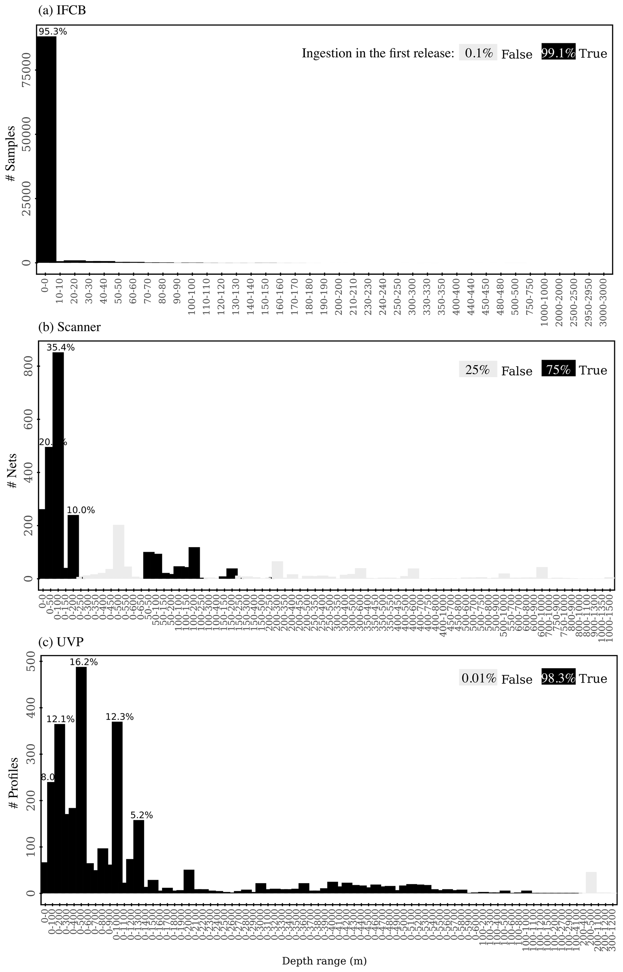
Figure A1Distribution of the sampling depth ranges of accessible (all bars) and ingested (black bars) IFCB (a), scanners (b), and UVP (c) datasets. Note that depth limits were rounded to a 10, 50, and 100 m resolution to reduce the number of ranges reported.
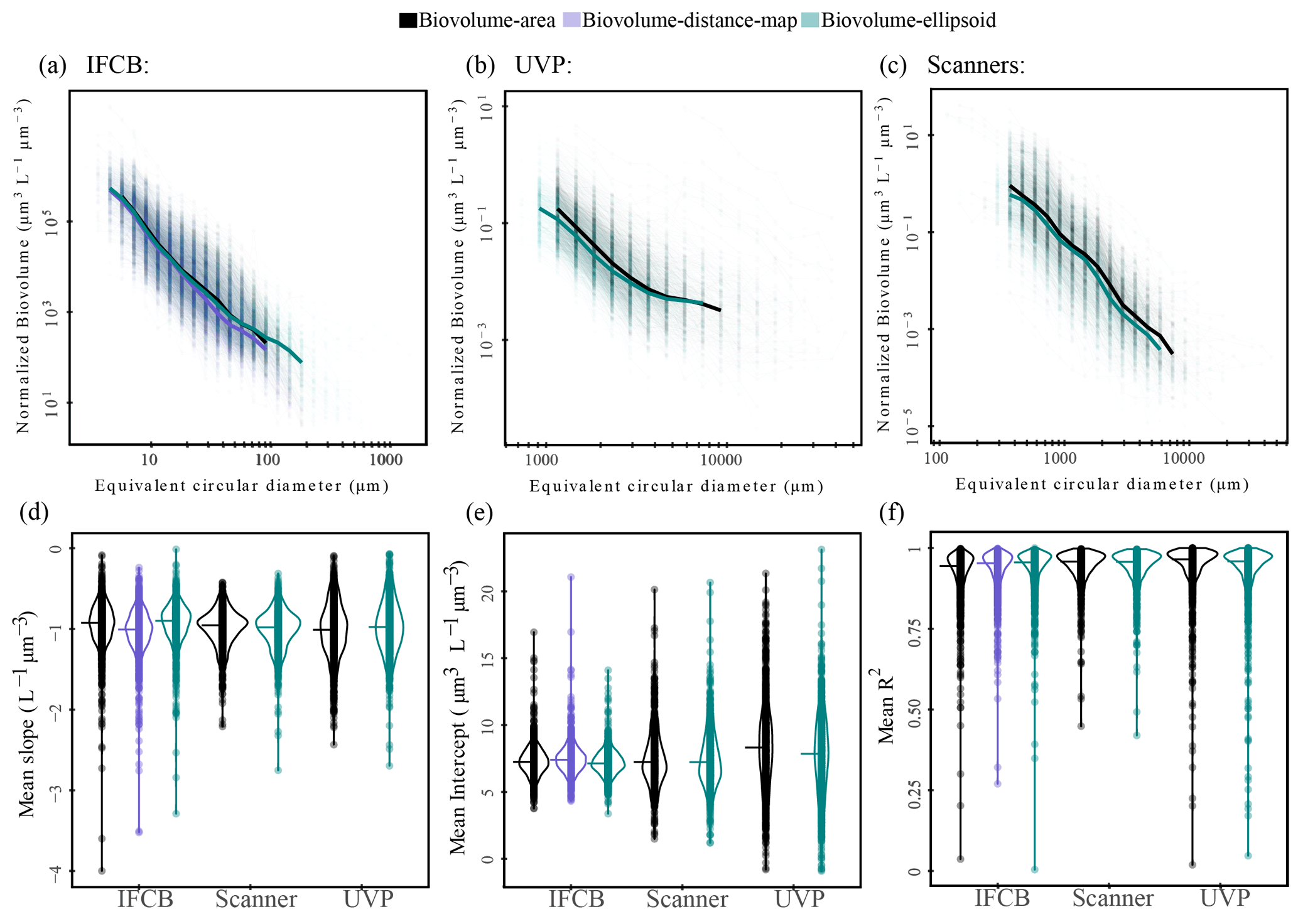
Figure A2Normalized biovolume size spectra (a–c) and associated linear regression parameters (d–f) calculated from three methods: area-based biovolume (this study, black); distance-map-based biovolume (Moberg and Sosik, 2012, light purple), which is part of the processing pipeline of the IFCB images; and ellipsoidal biovolume (aquamarine), which is more commonly used for processing ZooScan and UVP datasets. Dots represent individual samples (defined by temporal and spatial bins); solid lines in panels (a), (b), and (c) represent the median spectrum for the size classes that were present in at least 50 % of the samples (to avoid misalignments due to different sampling efforts). Violin plots in panels (d), (e), and (f) represent data density on the y axis, and horizontal lines represent the median. The data included in this analysis are restricted to particles that have length estimates for both the major and minor axes, resulting in only large particles being uploaded to EcoTaxa for the UVP datasets.
A2 Underwater Vision Profiler (UVP)
The fifth generation of the UVP (hereafter UVP5) consists of a system of two red LED lights (625 nm) that illuminate a 22×18 cm frame, which is imaged by a camera with a resolution of ∼8 pixels per mm facing the illuminated plane. This system was routinely mounted on CTD-rosettes (Picheral et al., 2010) before its miniaturization led to the next generation of UVPs (UVP6, Picheral et al., 2022). Both UVP5 and UVP6 are rated to 6000 m depth. UVP6 instruments only have one red LED light and image a smaller frame (15×18 cm) with a higher resolution (∼12 pixels per mm). As a result of its miniaturization, the UVP6 can be mounted on autonomous platforms like gliders, floats, or moorings to record images at a preset time interval, although acquisitions have mostly been done in profiling mode so far (Fig. A1). Upon descent, pressure sensor readings and images are recorded at a frequency of 6 to 20 Hz, depending on the configuration setting and the in situ concentration of particles, whereby low concentrations require less buffering time before each new acquisition and hence allow a higher acquisition frequency. The configuration setting allows users to record the raw image frames, the vignettes of particles larger than a fixed size threshold generated after segmentation (i.e., the process of extracting individual ROIs from the initial image), or a combination of both (full process mode). The size threshold is typically set to 44±22 pixels ( µm in equivalent circular diameter or ECD) and 70±15 pixels ( µm in ECD) for the UVP5 and UVP6, respectively. In mixed acquisition mode (the recommended setting to limit processing time during and following deployment), image frames are segmented in real time to extract the individual area and the mean gray-level estimates for each particle larger than 1 pixel ( and µm in ECD for UVP5 and UVP6, respectively), and vignettes of larger particles are saved as BMP thumbnails. Post-recovery, the metadata are manually filled, and the vignettes' BMP files are converted to binary masks whose morphometric features, including area and ellipsoidal axis, are extracted by a custom ImageJ toolbox named Zooprocess (Gorsky et al., 2010) for the UVP5 or via the UVP app for the UVP6 (Picheral et al., 2022). Size estimates for all particles can be further stored in EcoPart (https://ecopart.obs-vlfr.fr, last access: October 2023), while vignettes can be uploaded to the collaborative platform EcoTaxa (https://ecotaxa.obs-vlfr.fr, last access: October 2023) for automatic class predictions and manual validation. Prior to instrument shipping, both the effective volume (0.98±0.18 L for UVP5 and 0.6±0.02 L for UVP6) of the image frame and the two size conversion factors, Aa (the intercept) and Exp (the slope), linking metric-based area estimates to pixel-based area estimates by a power-law function, are calibrated against the unique reference unit (Picheral et al., 2010, 2022). However, the size conversion factors are used to account for light scattering around small particles only and are not required for size estimates of large particles, and the use of these factors can result in larger error propagation compared to a fixed pixel size conversion factor (data not shown). Therefore, all pixel-based area estimates were converted to metric area using a fixed pixel size factor (corresponding to the camera resolution reported above) for the UVP data included in the current PSSdb version. For further details regarding UVP data processing, see Kiko et al. (2022).
A3 Net sampling and benchtop scanners
Traditionally, zooplankton samples are collected via a wide range of net systems (reviewed by Wiebe and Benfield, 2003), preserved with a fixative reagent (mostly a buffered formaldehyde seawater solution), and processed in the laboratory. Benchtop flatbed scanning systems allow for a relatively high sample throughput compared to the traditional microscopic approach. PSSdb currently includes data collected from vertical or oblique tows with nets of various mesh sizes and aperture diameters (Fig. A1), mostly equipped with flow meters, and analyzed with the ZooScan system (Gorsky et al., 2010) or alternative generic scanners (Gislason and Silva, 2009; Lehette and Hernández-León, 2009; Kiko et al., 2020). These benchtop scanners have a resolution of ∼96 pixels per mm, with the frame being illuminated from above and scanned from below. These scanners are typically used to scan and digitize preserved zooplankton samples as the organisms must be immobile during scanning. Prior to scanning, a background image of the frame filled with distilled water is scanned to facilitate ROI segmentation. The samples are typically rinsed to remove the fixative and the seawater, size-fractionated using sieves of various mesh sizes, and subsampled into aliquots to reduce the number of organisms per scan and to avoid overlapping objects in the image (Jalabert et al., 2022). Similarly to UVP5 profiles, Zooprocess is used to save the scanner frame and to manually fill the metadata of each sample, including the GPS coordinates, sampling depth range, sampling time, volume of filtered seawater, and dilution factor of the scanned subsamples. Each scan will generate three files, containing the log, the metadata, and the overall scan saved as TIFF files. A first segmentation is performed to separate the ROIs from the background and to extract their morphometric features (see supplemental material of Gorsky et al., 2010), depending on a lower size threshold (370±360 µm in ECD on average) and the mean gray-level intensity (default is 243). If necessary, a second segmentation may be done after manually separating overlapping ROIs (Vandromme et al., 2012). Once the separation of ROIs is optimal, their corresponding vignettes, along with the automatically generated EcoTaxa table, may be uploaded to EcoTaxa to predict and validate the taxonomic annotations. As a starting point and for reproducibility, we only ingested datasets uploaded on EcoTaxa as they can be repeatedly accessed and shared amongst collaborators, notably to assess the annotation status, which is important for ingestion into PSSdb (see Sect. 2.2.4). Once datasets are exported from EcoTaxa, we consider the reported size-based fractionation of the net tow sample: if the sample was sieved into separate size fractions after the collection, (i.e., a sample collected with a 333 µm mesh net that was subsequently sieved through 150 µm, 500 µm and 1 mm meshes), the size spectra are first calculated for each size fraction based on the dilution factor of the aliquots taken for each sieved sample (“acq_sub_part” column in EcoTaxa) and the volume of filtered seawater of the net (as determined by the flowmeter; “sample_tot_vol” column in EcoTaxa) to account for the volume effectively scanned within a size fraction. The total size spectrum is then obtained by summing the fraction-specific spectra since size-fractionated scans originate from the same volume.
MD, MCU, JYL, RK, TDO'B, JOI, FL, LS, and CS contributed to the conception and primary efforts (data compilation, quality controlling, and computation) leading to the release and publication of the Pelagic Size Structure database. RK, JOI, FL, LS, CRA, AC, LG, CG, HH, LKB, RMK, AM, MN, MP, JBR, and HMS led the data acquisition. MB, NB, SB, FC, ETC, PD, CD, LD, AE, AF, NG, PLG, KH, JAH, LJ, KMK, ML, CM, ZM, BN, TP, EP, ER, CR, GS, JT, CT, and MV contributed to the data collection, acquisition, analysis, or curation. All the authors contributed to and approve of the paper.
The contact author has declared that none of the authors has any competing interests.
Publisher's note: Copernicus Publications remains neutral with regard to jurisdictional claims made in the text, published maps, institutional affiliations, or any other geographical representation in this paper. While Copernicus Publications makes every effort to include appropriate place names, the final responsibility lies with the authors.
This work was mainly funded by NOAA (award no. NA21OAR4310254 to Jessica Y. Luo, Rainer Kiko, Lars Stemmann, Fabien Lombard, Jean-Olivier Irisson, Todd D. O'Brien, and Charles Stock) under the project “Developing PSSdb: a Pelagic Size Structure database to support biogeochemical modelling”. Mathilde Dugenne, Rainer Kiko, and Lars Stemmann received further support from the European Union's project TRIATLAS (European Union Horizon 2020 program, grant agreement no. 817578). Rainer Kiko additionally acknowledges support from a Make Our Planet Great Again grant from the French National Research Agency (ANR) within the Programme d'Investissements d'Avenir (grant no. ANR-19-MPGA-0012) and from the Heisenberg Programme of the German Science Foundation (grant no. KI 1387/5-1). We acknowledge the support of the California IFCB database through the NOAA Prevention, Control, and Mitigation of Harmful Algal Blooms award (no. NA20NOS4780187).
This research has been supported by the National Oceanic and Atmospheric Administration (grant no. NA21OAR4310254), the European Union Horizon 2020 (grant no. 817578), the Agence Nationale de la Recherche (grant no. ANR-19-MPGA-0012), and the Deutsche Forschungsgemeinschaft (grant no. KI 1387/5-1).
This paper was edited by François G. Schmitt and reviewed by two anonymous referees.
Andersen, K. H., Berge, T., Gonçalves, R. J., Hartvig, M., Heuschele, J., Hylander, S., Jacobsen, N. S., Lindemann, C., Martens, E. A., Neuheimer, A. B., Olsson, K., Palacz, A., Prowe, A. E. F., Sainmont, J., Traving, S. J., Visser, A. W., Wadhwa, N., and Kiørboe, T.: Characteristic sizes of life in the oceans, from bacteria to whales, Annu. Rev. Mar. Sci., 8, 217–241, 2016. a
Armstrong, R. A. and McGehee, R.: Competitive Exclusion, Am. Nat., 115, 151–170, 1980. a
Armstrong, R. A., Lee, C., Hedges, J. I., Honjo, S., and Wakeham, S. G.: A new, mechanistic model for organic carbon fluxes in the ocean based on the quantitative association of POC with ballast minerals, Deep-Sea Res. Pt. II, 49, 219–236, https://doi.org/10.1016/S0967-0645(01)00101-1, 2001. a
Atkinson, A., Lilley, M. K., Hirst, A. G., McEvoy, A. J., Tarran, G. A., Widdicombe, C., Fileman, E. S., Woodward, E. M. S., Schmidt, K., Smyth, T. J., and Somerfield, P. J.: Increasing nutrient stress reduces the efficiency of energy transfer through planktonic size spectra, Limnol. Oceanogr., 66, 422–437, https://doi.org/10.1002/lno.11613, 2021. a, b, c, d
Atkinson, A., Rossberg, A. G., Gaedke, U., Sprules, G., Heneghan, R. F., Batziakas, S., Grigoratou, M., Fileman, E., Schmidt, K., and Frangoulis, C.: Steeper size spectra with decreasing phytoplankton biomass indicate strong trophic amplification and future fish declines, Nat. Commun., 15, 381, https://doi.org/10.1038/s41467-023-44406-5, 2024. a, b
Banas, N. S.: Adding complex trophic interactions to a size-spectral plankton model: Emergent diversity patterns and limits on predictability, Ecol. Model., 222, 2663–2675, https://doi.org/10.1016/j.ecolmodel.2011.05.018, 2011. a
Barton, A. D., Finkel, Z. V., Ward, B. A., Johns, D. G., and Follows, M. J.: On the roles of cell size and trophic strategy in North Atlantic diatom and dinoflagellate communities, Limnol. Oceanogr., 58, 254–266, https://doi.org/10.4319/lo.2013.58.1.0254, 2013. a
Basu, S. and Mackey, K.: Phytoplankton as Key Mediators of the Biological Carbon Pump: Their Responses to a Changing Climate, Sustainability, 10, 869, https://doi.org/10.3390/su10030869, 2018. a
Batten, S. D., Abu-Alhaija, R., Chiba, S., Edwards, M., Graham, G., Jyothibabu, R., Kitchener, J. A., Koubbi, P., McQuatters-Gollop, A., Muxagata, E., Ostle, C., Richardson, A. J., Robinson, K. V., Takahashi, K. T., Verheye, H. M., and Wilson, W.: A Global Plankton Diversity Monitoring Program, Front. Mar. Sci., 6, 321, https://doi.org/10.3389/fmars.2019.00321, 2019. a
Biard, T., Stemmann, L., Picheral, M., Mayot, N., Vandromme, P., Hauss, H., Gorsky, G., Guidi, L., Kiko, R., and Not, F.: In situ imaging reveals the biomass of giant protists in the global ocean, Nature, 532, 504–507, https://doi.org/10.1038/nature17652, 2016. a, b
Bisson, K. M., Kiko, R., Siegel, D. A., Guidi, L., Picheral, M., Boss, E., and Cael, B. B.: Sampling uncertainties of particle size distributions and derived fluxes, Limnol. Oceanogr.-Methods, 20, 754–767, https://doi.org/10.1002/lom3.10524, 2022. a
Boyd, P. and Newton, P.: Does planktonic community structure determine downward particulate organic carbon flux in different oceanic provinces?, Deep-Sea Res. Pt. I, 46, 63–91, 1999. a
Buitenhuis, E. T., Vogt, M., Moriarty, R., Bednaršek, N., Doney, S. C., Leblanc, K., Le Quéré, C., Luo, Y.-W., O'Brien, C., O'Brien, T., Peloquin, J., Schiebel, R., and Swan, C.: MAREDAT: towards a world atlas of MARine Ecosystem DATa, Earth Syst. Sci. Data, 5, 227–239, https://doi.org/10.5194/essd-5-227-2013, 2013. a
Cael, B. B., Cavan, E. L., and Britten, G. L.: Reconciling the Size-Dependence of Marine Particle Sinking Speed, Geophys. Res. Lett., 48, e2020GL091771, https://doi.org/10.1029/2020GL091771, 2021. a
Cavender-Bares, K. K., Rinaldo, A., and Chisholm, S. W.: Microbial size spectra from natural and nutrient enriched ecosystems, Limnol. Oceanogr., 46, 778–789, https://doi.org/10.4319/lo.2001.46.4.0778, 2001. a
Chen, B. and Liu, H.: Relationships between phytoplankton growth and cell size in surface oceans: Interactive effects of temperature, nutrients, and grazing, Limnol. Oceanogr., 55, 965–972, https://doi.org/10.4319/lo.2010.55.3.0965, 2010. a
Chiba, S., Batten, S., Martin, C. S., Ivory, S., Miloslavich, P., and Weatherdon, L. V.: Zooplankton monitoring to contribute towards addressing global biodiversity conservation challenges, J. Plankton Res., 40, 509–518, https://doi.org/10.1093/plankt/fby030, 2018. a
Chisholm, S. W.: Phytoplankton Size, in: Primary Productivity and Biogeochemical Cycles in the Sea, edited by: Falkowski, P. G., Woodhead, A. D., and Vivirito, K., Environmental Science Research, vol. 43, Springer, Boston, MA, https://doi.org/10.1007/978-1-4899-0762-2_12, 1992. a, b
Choi, H. Y., Stewart, G. M., Lomas, M. W., Kelly, R. P., and Moran, S. B.: Linking the distribution of 210Po and 210Pb with plankton community along Line P, Northeast Subarctic Pacific, J. Environ. Radioact., 138, 390–401, https://doi.org/10.1016/j.jenvrad.2014.02.009, 2014. a
Claustre, H., Johnson, K. S., and Takeshita, Y.: Observing the global ocean with biogeochemical-Argo, Annu. Rev. Mar. Sci., 12, 23–48, 2020. a, b
Clayton, S., Alexander, H., Graff, J. R., Poulton, N. J., Thompson, L. R., Benway, H., Boss, E., and Martiny, A.: Bio-GO-SHIP: The Time Is Right to Establish Global Repeat Sections of Ocean Biology, Front. Mar. Sci., 8, 767443, https://doi.org/10.3389/fmars.2021.767443, 2022. a
Clements, D. J., Yang, S., Weber, T., McDonnell, A. M. P., Kiko, R., Stemmann, L., and Bianchi, D.: Constraining the Particle Size Distribution of Large Marine Particles in the Global Ocean With In Situ Optical Observations and Supervised Learning, Global Biogeochem. Cycles, 36, e2021GB007276, https://doi.org/10.1029/2021GB007276, 2022. a, b
Colas, F., Tardivel, M., Perchoc, J., Lunven, M., Forest, B., Guyader, G., Danielou, M., Le Mestre, S., Bourriau, P., Antajan, E., Sourisseau, M., Huret, M., Petitgas, P., and Romagnan, J.: The ZooCAM, a new in-flow imaging system for fast onboard counting, sizing and classification of fish eggs and metazooplankton, Prog. Oceanogr., 166, 54–65, https://doi.org/10.1016/j.pocean.2017.10.014, 2018. a
Cowen, R. K. and Guigand, C. M.: In situ ichthyoplankton imaging system (I SIIS): system design and preliminary results: In situ ichthyoplankton imaging system, Limnol. Oceanogr.-Methods, 6, 126–132, https://doi.org/10.4319/lom.2008.6.126, 2008. a, b
Davis, C. S., Thwaites, F. T., Gallager, S. M., and Hu, Q.: A three-axis fast-tow digital Video Plankton Recorder for rapid surveys of plankton taxa and hydrography: New Video Plankton Recorder, Limnol. Oceanogr.-Methods, 3, 59–74, https://doi.org/10.4319/lom.2005.3.59, 2005. a, b, c
Dubelaar, G. B. and Gerritzen, P. L.: CytoBuoy: a step forward towards using flow cytometry in operational oceanography, Sci. Mar., 64, 255–265, https://doi.org/10.3989/scimar.2000.64n2255, 2000. a
Dubois, C., Irisson, J., and Debreuve, E.: Correcting estimations of copepod volume from two-dimensional images, Limnol. Oceanogr.-Methods, 20, 361–371, https://doi.org/10.1002/lom3.10492, 2022. a, b
Dugenne, M., Corrales-Ugalde, M., Luo, J. Y., Stemmann, L., Irisson, J.-O., Lombard, F., O'Brien, T., Stock, C., Consortium, P. D. C., and Kiko, R.: Key link between iron and the size structure of three main mesoplanktonic groups (Crustaceans, Rhizarians, and colonial N2-fixers) in the Global Ocean, Section: New Results, 2024.03.08.584097, https://doi.org/10.1101/2024.03.08.584097, 2024a. a
Dugenne, M., Corrales-Ugalde, M., O'Brien, T., Lombard, F., Irisson, J.-O., Stemmann, L., Stock, C., Kiko, R., and Luo, J. Y.: A Pelagic Size Structure database (PSSdb) to support biogeochemical modeling: second update to first release, Zenodo [data set], https://doi.org/10.5281/zenodo.10809693 (last access: April 2024), 2024b. a, b, c, d, e, f
Durkin, C. A., Estapa, M. L., and Buesseler, K. O.: Observations of carbon export by small sinking particles in the upper mesopelagic, Mar. Chem., 175, 72–81, https://doi.org/10.1016/j.marchem.2015.02.011, 2015. a, b
Durkin, C. A., Buesseler, K. O., Cetinić, I., Estapa, M. L., Kelly, R. P., and Omand, M.: A Visual Tour of Carbon Export by Sinking Particles, Global Biogeochem. Cycles, 35, e2021GB006985, https://doi.org/10.1029/2021GB006985, 2021. a
Edwards, K. F., Thomas, M. K., Klausmeier, C. A., and Litchman, E.: Allometric scaling and taxonomic variation in nutrient utilization traits and maximum growth rate of phytoplankton, Limnol. Oceanogr., 57, 554–566, https://doi.org/10.4319/lo.2012.57.2.0554, 2012. a
Eerola, T., Batrakhanov, D., Barazandeh, N. V., Kraft, K., Haraguchi, L., Lensu, L., Suikkanen, S., Seppälä, J., Tamminen, T., and Kälviäinen, H.: Survey of Automatic Plankton Image Recognition: Challenges, Existing Solutions and Future Perspectives, https://doi.org/10.48550/arXiv.2305.11739, arXiv:2305.11739 [cs], 2023. a
Finkel, Z. V., Vaillancourt, C. J., Irwin, A. J., Reavie, E. D., and Smol, J. P.: Environmental control of diatom community size structure varies across aquatic ecosystems, Proc. Royal Soc. B., 276, 1627–1634, 2009. a
Fischer, A. D., Hayashi, K., McGaraghan, A., and Kudela, R. M.: Return of the “age of dinoflagellates” in Monterey Bay: Drivers of dinoflagellate dominance examined using automated imaging flow cytometry and long-term time series analysis, Limnol. Oceanogr., 65, 2125–2141, https://doi.org/10.1002/lno.11443, 2020. a, b
Gallager, S. M.: The Continuous Plankton Imaging and Classification Sensor (CPICS): A Sensor for Quantifying Mesoplankton Biodiversity and Community Structure, 2016, IS52A–07, American Geophysical Union, 2016AGUOSIS52A..07G, https://ui.adsabs.harvard.edu/abs/2016AGUOSIS52A..07G (last access: October 2023), 2016. a, b
García-Comas, C., Stemmann, L., Ibanez, F., Berline, L., Mazzocchi, M. G., Gasparini, S., Picheral, M., and Gorsky, G.: Zooplankton long-term changes in the NW Mediterranean Sea: Decadal periodicity forced by winter hydrographic conditions related to large-scale atmospheric changes?, J. Mar. Syst., 87, 216–226, https://doi.org/10.1016/j.jmarsys.2011.04.003, 2011. a
Gislason, A. and Silva, T.: Comparison between automated analysis of zooplankton using ZooImage and traditional methodology, J. Plankton Res., 31, 1505–1516, https://doi.org/10.1093/plankt/fbp094, 2009. a, b
Glibert, P. M.: Harmful algae at the complex nexus of eutrophication and climate change, Harmful Algae, 91, 101583, https://doi.org/10.1016/j.hal.2019.03.001, 2020. a
Gorsky, G., Ohman, M. D., Picheral, M., Gasparini, S., Stemmann, L., Romagnan, J.-B., Cawood, A., Pesant, S., Garcia-Comas, C., and Prejger, F.: Digital zooplankton image analysis using the ZooScan integrated system, J. Plankton Res., 32, 285–303, https://doi.org/10.1093/plankt/fbp124, 2010. a, b, c, d, e, f
Grandrémy, N., Bourriau, P., Daché, E., Danielou, M.-M., Doray, M., Dupuy, C., Huret, M., Jalabert, L., Le Mestre, S., Nowaczyk, A., Petitgas, P., Pineau, P., Raphalen, E., and Romagnan, J.-B.: PELGAS Bay of Biscay ZooScan zooplankton Dataset (2004–2016), SEANOE [data set], https://doi.org/10.17882/94052, 2023a. a, b
Grandrémy, N., Bourriau, P., Danielou, M.-M., Doray, M., Dupuy, C., Forest, B., Huret, M., Le Mestre, S., Nowacyk, A., Petitgas, P., Pineau, P., Rouxel, J., Tardivel, M., and Romagnan, J.-B.: PELGAS Bay of Biscay ZooCAM zooplankton Dataset (2016–2019), SEANOE [data set], https://doi.org/10.17882/94040, 2023b. a
Grandrémy, N., Romagnan, J.-B., Dupuy, C., Doray, M., Huret, M., and Petitgas, P.: Hydrology and small pelagic fish drive the spatio-temporal dynamics of springtime zooplankton assemblages over the Bay of Biscay continental shelf, Prog. Oceanogr., 210, 102949, https://doi.org/10.1016/j.pocean.2022.102949, 2023c. a, b
Grandremy, N., Bourriau, P., Daché, E., Danielou, M.-M., Doray, M., Dupuy, C., Forest, B., Jalabert, L., Huret, M., Le Mestre, S., Nowaczyk, A., Petitgas, P., Pineau, P., Rouxel, J., Tardivel, M., and Romagnan, J.-B.: Metazoan zooplankton in the Bay of Biscay: a 16-year record of individual sizes and abundances obtained using the ZooScan and ZooCAM imaging systems, Earth Syst. Sci. Data, 16, 1265–1282, https://doi.org/10.5194/essd-16-1265-2024, 2024. a
Guidi, L., Stemmann, L., Jackson, G. A., Ibanez, F., Claustre, H., Legendre, L., Picheral, M., and Gorskya, G.: Effects of phytoplankton community on production, size, and export of large aggregates: A world-ocean analysis, Limnol. Oceanogr., 54, 1951–1963, https://doi.org/10.4319/lo.2009.54.6.1951, 2009. a
Guidi, L., Chaffron, S., Bittner, L., Eveillard, D., Larhlimi, A., Roux, S., Darzi, Y., Audic, S., Berline, L., Brum, J. R., Coelho, L. P., Espinoza, J. C. I., Malviya, S., Sunagawa, S., Dimier, C., Kandels-Lewis, S., Picheral, M., Poulain, J., Searson, S., Tara Oceans Consortium Coordinators, Stemmann, L., Not, F., Hingamp, P., Speich, S., Follows, M., Karp-Boss, L., Boss, E., Ogata, H., Pesant, S., Weissenbach, J., Wincker, P., Acinas, S. G., Bork, P., De Vargas, C., Iudicone, D., Sullivan, M. B., Raes, J., Karsenti, E., Bowler, C., and Gorsky, G.: Plankton networks driving carbon export in the oligotrophic ocean, Nature, 532, 465–470, https://doi.org/10.1038/nature16942, 2016. a
Hansen, B., Bjornsen, P. K., and Hansen, P. J.: The size ratio between planktonic predators and their prey, Limnol. Oceanogr., 39, 395–403, https://doi.org/10.4319/lo.1994.39.2.0395, 1994. a, b
Harred, L. B. and Campbell, L.: Predicting harmful algal blooms: a case study with Dinophysis ovum in the Gulf of Mexico, J. Plankton Res., 36, 1434–1445, https://doi.org/10.1093/plankt/fbu070, 2014. a
Hatton, I. A., Heneghan, R. F., Bar-On, Y. M., and Galbraith, E. D.: The global ocean size spectrum from bacteria to whales, Sci. Adv., 7, eabh3732, https://doi.org/10.1126/sciadv.abh3732, 2021. a, b, c, d, e
Hauss, H., Schwabe, L., and Peck, M. A.: The costs and trade-offs of optimal foraging in marine fish larvae, J. Anim. Ecol., 92, 1016–1028, https://doi.org/10.1111/1365-2656.13915, 2023. a
Haëntjens, N., Boss, E. S., Graff, J. R., Chase, A. P., and Karp-Boss, L.: Phytoplankton size distributions in the western North Atlantic and their seasonal variability, Limnol. Oceanogr., 67, 1865–1878, https://doi.org/10.1002/lno.12172, 2022. a, b, c
Hillebrand, H., Acevedo-Trejos, E., Moorthi, S. D., Ryabov, A., Striebel, M., Thomas, P. K., and Schneider, M.-L.: Cell size as driver and sentinel of phytoplankton community structure and functioning, Funct. Ecol., 36, 276–293, 2022. a, b
Hirata, T., Hardman-Mountford, N. J., Brewin, R. J. W., Aiken, J., Barlow, R., Suzuki, K., Isada, T., Howell, E., Hashioka, T., Noguchi-Aita, M., and Yamanaka, Y.: Synoptic relationships between surface Chlorophyll-a and diagnostic pigments specific to phytoplankton functional types, Biogeosciences, 8, 311–327, https://doi.org/10.5194/bg-8-311-2011, 2011. a, b
Hirst, A. and Kiørboe, T.: Mortality of marine planktonic copepods: global rates and patterns, Mar. Ecol. Prog. Ser., 230, 195–209, https://doi.org/10.3354/meps230195, 2002. a
Hopcroft, R. R., Roff, J. C., Webber, M. K., and Witt, J. D. S.: Zooplankton growth rates: the influence of size and resources in tropical marine copepodites, Mar. Biol., 132, 67–77, https://doi.org/10.1007/s002270050372, 1998. a
Huete-Ortega, M., Cermeño, P., Calvo-Díaz, A., and Marañón, E.: Isometric size-scaling of metabolic rate and the size abundance distribution of phytoplankton, P. Roy. Soc. B., 279, 1815–1823, https://doi.org/10.1098/rspb.2011.2257, 2012. a
Ikeda, T.: Respiration and ammonia excretion by marine metazooplankton taxa: synthesis toward a global-bathymetric model, Mar. Biol., 161, 2753–2766, 2014. a
Irisson, J.-O., Ayata, S.-D., Lindsay, D. J., Karp-Boss, L., and Stemmann, L.: Machine learning for the study of plankton and marine snow from images, Annu. Rev. Mar. Sci., 14, 277–301, 2022. a
Jalabert, L., Picheral, M., Desnos, C., and Elineau, A.: ZooScan Protocol, https://www.protocols.io/view/zooscan-protocol-bziyp4fw (last access: October 2023), 2022. a
Jonasz, M. and Fournier, G.: Approximation of the size distribution of marine particles by a sum of log-normal functions, Limnol. Oceanogr., 41, 744–754, https://doi.org/10.4319/lo.1996.41.4.0744, 1996. a
Juranek, L. W., White, A. E., Dugenne, M., Henderikx Freitas, F., Dutkiewicz, S., Ribalet, F., Ferrón, S., Armbrust, E. V., and Karl, D. M.: The Importance of the Phytoplankton “Middle Class” to Ocean Net Community Production, Global Biogeochem. Cycles, 34, e2020GB006702, https://doi.org/10.1029/2020GB006702, 2020. a
Kiko, R., Biastoch, A., Brandt, P., Cravatte, S., Hauss, H., Hummels, R., Kriest, I., Marin, F., McDonnell, A. M. P., Oschlies, A., Picheral, M., Schwarzkopf, F. U., Thurnherr, A. M., and Stemmann, L.: Biological and physical influences on marine snowfall at the equator, Nat. Geosci, 10, 852–858, 2017. a
Kiko, R., Brandt, P., Christiansen, S., Faustmann, J., Kriest, I., Rodrigues, E., Schütte, F., and Hauss, H.: Zooplankton-Mediated Fluxes in the Eastern Tropical North Atlantic, Front. Mar. Sci., 7, 358, https://doi.org/10.3389/fmars.2020.00358, 2020. a, b
Kiko, R., Picheral, M., Antoine, D., Babin, M., Berline, L., Biard, T., Boss, E., Brandt, P., Carlotti, F., Christiansen, S., Coppola, L., de la Cruz, L., Diamond-Riquier, E., Durrieu de Madron, X., Elineau, A., Gorsky, G., Guidi, L., Hauss, H., Irisson, J.-O., Karp-Boss, L., Karstensen, J., Kim, D., Lekanoff, R. M., Lombard, F., Lopes, R. M., Marec, C., McDonnell, A. M. P., Niemeyer, D., Noyon, M., O'Daly, S. H., Ohman, M. D., Pretty, J. L., Rogge, A., Searson, S., Shibata, M., Tanaka, Y., Tanhua, T., Taucher, J., Trudnowska, E., Turner, J. S., Waite, A., and Stemmann, L.: A global marine particle size distribution dataset obtained with the Underwater Vision Profiler 5, Earth Syst. Sci. Data, 14, 4315–4337, https://doi.org/10.5194/essd-14-4315-2022, 2022. a, b, c, d, e, f, g, h, i
Kiørboe, T. and Hirst, A. G.: Shifts in Mass Scaling of Respiration, Feeding, and Growth Rates across Life-Form Transitions in Marine Pelagic Organisms, Am. Nat., 183, E118–E130, https://doi.org/10.1086/675241, 2014. a, b
Kostadinov, T. S., Siegel, D. A., and Maritorena, S.: Retrieval of the particle size distribution from satellite ocean color observations, J. Geophys. Res., 114, C09015, https://doi.org/10.1029/2009JC005303, 2009. a, b, c
Kostadinov, T. S., Robertson Lain, L., Kong, C. E., Zhang, X., Maritorena, S., Bernard, S., Loisel, H., Jorge, D. S. F., Kochetkova, E., Roy, S., Jonsson, B., Martinez-Vicente, V., and Sathyendranath, S.: Ocean color algorithm for the retrieval of the particle size distribution and carbon-based phytoplankton size classes using a two-component coated-sphere backscattering model, Ocean Sci., 19, 703–727, https://doi.org/10.5194/os-19-703-2023, 2023. a
Kraft, K., Velhonoja, O., Eerola, T., Suikkanen, S., Tamminen, T., Haraguchi, L., Ylöstalo, P., Kielosto, S., Johansson, M., Lensu, L., Kälviäinen, H., Haario, H., and Seppälä, J.: Towards operational phytoplankton recognition with automated high-throughput imaging, near-real-time data processing, and convolutional neural networks, Front. Mar. Sci., 9, 867695, https://doi.org/10.3389/fmars.2022.867695, 2022. a, b
Leblanc, K., Quéguiner, B., Diaz, F., Cornet, V., Michel-Rodriguez, M., Durrieu De Madron, X., Bowler, C., Malviya, S., Thyssen, M., Grégori, G., Rembauville, M., Grosso, O., Poulain, J., De Vargas, C., Pujo-Pay, M., and Conan, P.: Nanoplanktonic diatoms are globally overlooked but play a role in spring blooms and carbon export, Nat. Commun., 9, 953, https://doi.org/10.1038/s41467-018-03376-9, 2018. a
Legendre, L. and Le Fèvre, J.: Microbial food webs and the export of biogenic carbon in oceans, Aquat. Microb. Ecol., 09, 69–77, https://doi.org/10.3354/ame009069, 1995. a
Lehette, P. and Hernández-León, S.: Zooplankton biomass estimation from digitized images: a comparison between subtropical and Antarctic organisms, Limnol. Oceanogr.-Methods, 7, 304–308, https://doi.org/10.4319/lom.2009.7.304, 2009. a, b, c
Ljungström, G., Claireaux, M., Fiksen, Ã., and Jørgensen, C.: Body size adaptions under climate change: zooplankton community more important than temperature or food abundance in model of a zooplanktivorous fish, Mar. Ecol. Prog. Ser., 636, 1–18, https://doi.org/10.3354/meps13241, 2020. a
Lomas, M. W. and Moran, S. B.: Evidence for aggregation and export of cyanobacteria and nano-eukaryotes from the Sargasso Sea euphotic zone, Biogeosciences, 8, 203–216, https://doi.org/10.5194/bg-8-203-2011, 2011. a
Lombard, F., Boss, E., Waite, A. M., Vogt, M., Uitz, J., Stemmann, L., Sosik, H. M., Schulz, J., Romagnan, J.-B., Picheral, M., Pearlman, J., Ohman, M. D., Niehoff, B., Möller, K. O., Miloslavich, P., Lara-Lpez, A., Kudela, R., Lopes, R. M., Kiko, R., Karp-Boss, L., Jaffe, J. S., Iversen, M. H., Irisson, J.-O., Fennel, K., Hauss, H., Guidi, L., Gorsky, G., Giering, S. L. C., Gaube, P., Gallager, S., Dubelaar, G., Cowen, R. K., Carlotti, F., Briseño-Avena, C., Berline, L., Benoit-Bird, K., Bax, N., Batten, S., Ayata, S. D., Artigas, L. F., and Appeltans, W.: Globally consistent quantitative observations of planktonic ecosystems, Front. Mar. Sci., 6, 196, https://doi.org/10.3389/fmars.2019.00196, 2019. a, b, c, d, e, f, g, h
Luo, J. Y., Irisson, J.-O., Graham, B., Guigand, C., Sarafraz, A., Mader, C., and Cowen, R. K.: Automated plankton image analysis using convolutional neural networks, Limnol. Oceanogr.-Methods, 16, 814–827, 2018. a
Luo, J. Y., Corrales-Ugalde, M., Dugenne, M., and Kiko, R.: jessluo/PSSdb: A Pelagic Size Structure database (PSSdb) to support biogeochemical modeling: third update to first release (v2024-04), Zenodo [code], https://doi.org/10.5281/zenodo.11983391, 2024. a
Maas, A. E., Miccoli, A., Stamieszkin, K., Carlson, C. A., and Steinberg, D. K.: Allometry and the calculation of zooplankton metabolism in the subarctic Northeast Pacific Ocean, J. Plankton Res., 43, 413–427, https://doi.org/10.1093/plankt/fbab026, 2021. a
Marañón, E., Holligan, P., Barciela, R., González, N., Mouriño, B., Pazó, M., and Varela, M.: Patterns of phytoplankton size structure and productivity in contrasting open-ocean environments, Mar. Ecol. Prog. Ser., 216, 43–56, https://doi.org/10.3354/meps216043, 2001. a
Marcolin, C. D. R., Schultes, S., Jackson, G. A., and Lopes, R. M.: Plankton and seston size spectra estimated by the LOPC and ZooScan in the Abrolhos Bank ecosystem (SE Atlantic), Cont. Shelf Res., 70, 74–87, https://doi.org/10.1016/j.csr.2013.09.022, 2013. a
Martin-Cabrera, P., Perez Perez, R., Irrison, J.-O., Lombard, F., Ove Möller, K., Rühl, S., Creach, V., Lindh, M., Stemmann, L., and Schepers, L.: Establishing Plankton Imagery Dataflows Towards International Biodiversity Data Aggregators, Biodiversity Information Science and Standards, 6, e94196, https://doi.org/10.3897/biss.6.94196, 2022. a
McConville, K., Atkinson, A., Fileman, E. S., Spicer, J. I., and Hirst, A. G.: Disentangling the counteracting effects of water content and carbon mass on zooplankton growth, J. Plankton Res., 39, 246–256, https://doi.org/10.1093/plankt/fbw094, 2017. a
Menden-Deuer, S. and Lessard, E. J.: Carbon to volume relationships for dinoflagellates, diatoms, and other protist plankton, Limnol. Oceanogr., 45, 569–579, https://doi.org/10.4319/lo.2000.45.3.0569, 2000. a
Menden-Deuer, S., Slade, W. H., and Dierssen, H.: Promoting Instrument Development for New Research Avenues in Ocean Science: Opening the Black Box of Grazing, Front. Mar. Sci., 8, 695938, https://doi.org/10.3389/fmars.2021.695938, 2021. a
Miloslavich, P., Bax, N. J., Simmons, S. E., Klein, E., Appeltans, W., Aburto-Oropeza, O., Andersen Garcia, M., Batten, S. D., Benedetti-Cecchi, L., Checkley, D. M., Chiba, S., Duffy, J. E., Dunn, D. C., Fischer, A., Gunn, J., Kudela, R., Marsac, F., Muller-Karger, F. E., Obura, D., and Shin, Y.: Essential ocean variables for global sustained observations of biodiversity and ecosystem changes, Global Change Biol., 24, 2416–2433, https://doi.org/10.1111/gcb.14108, 2018. a
Moberg, E. A. and Sosik, H. M.: Distance maps to estimate cell volume from two-dimensional plankton images: Distance map cell volume algorithm, Limnol. Oceanogr.-Methods, 10, 278–288, https://doi.org/10.4319/lom.2012.10.278, 2012. a, b, c
Moriarty, R. and O'Brien, T. D.: Distribution of mesozooplankton biomass in the global ocean, Earth Syst. Sci. Data, 5, 45–55, https://doi.org/10.5194/essd-5-45-2013, 2013. a
Moscoso, J. E., Bianchi, D., and Stewart, A. L.: Controls and characteristics of biomass quantization in size-structured planktonic ecosystem models, Ecol. Model., 468, 109907, https://doi.org/10.1016/j.ecolmodel.2022.109907, 2022. a, b
Neeley, A., Beaulieu, S. E., Proctor, C., Cetinić, I., Futrelle, J., Soto Ramos, I., Sosik, H. M., Devred, E., Karp-Boss, L., Picheral, M., Poulton, N., Roesler, C. S., and Shepherd, A.: Standards and practices for reporting plankton and other particle observations from images, Woods Hole Oceanographic Institution, https://hdl.handle.net/1912/27377 (last access: October 2023), 2021. a, b
Negrete-García, G., Luo, J. Y., Long, M. C., Lindsay, K., Levy, M., and Barton, A. D.: Plankton energy flows using a global size-structured and trait-based model, Prog. Oceanogr., 209, 102898, https://doi.org/10.1016/j.pocean.2022.102898, 2022. a
Noyon, M., Poulton, A. J., Asdar, S., Weitz, R., and Giering, S. L. C.: Mesozooplankton community distribution on the Agulhas Bank in autumn: Size structure and production, Deep-Sea Res. Pt. II, 195, 105015, https://doi.org/10.1016/j.dsr2.2021.105015, 2022. a
Ohman, M. D. and Romagnan, J.: Nonlinear effects of body size and optical attenuation on Diel Vertical Migration by zooplankton, Limnol. Oceanogr., 61, 765–770, https://doi.org/10.1002/lno.10251, 2016. a
Ohman, M. D., Davis, R. E., Sherman, J. T., Grindley, K. R., Whitmore, B. M., Nickels, C. F., and Ellen, J. S.: Zooglider: An autonomous vehicle for optical and acoustic sensing of zooplankton, Limnol. Oceanogr.-Methods, 17, 69–86, https://doi.org/10.1002/lom3.10301, 2019. a, b
Olson, R. J. and Sosik, H. M.: A submersible imaging-in-flow instrument to analyze nano-and microplankton: Imaging FlowCytobot: In situ imaging of nano- and microplankton, Limnol. Oceanogr.-Methods, 5, 195–203, https://doi.org/10.4319/lom.2007.5.195, 2007. a, b, c
Orenstein, E. C., Ayata, S.-D., Maps, F., Becker, Ã. C., Benedetti, F., Biard, T., de Garidel-Thoron, T., Ellen, J. S., Ferrario, F., Giering, S. L. C., Guy-Haim, T., Hoebeke, L., Iversen, M. H., Kiørboe, T., Lalonde, J.-F., Lana, A., Laviale, M., Lombard, F., Lorimer, T., Martini, S., Meyer, A., Möller, K. O., Niehoff, B., Ohman, M. D., Pradalier, C., Romagnan, J.-B., Schröder, S.-M., Sonnet, V., Sosik, H. M., Stemmann, L. S., Stock, M., Terbiyik-Kurt, T., Valcárcel-Pérez, N., Vilgrain, L., Wacquet, G., Waite, A. M., and Irisson, J.-O.: Machine learning techniques to characterize functional traits of plankton from image data, Limnol. Oceanogr., 67, 1647–1669, https://doi.org/10.1002/lno.12101, 2022. a
Picheral, M., Guidi, L., Stemmann, L., Karl, D. M., Iddaoud, G., and Gorsky, G.: The Underwater Vision Profiler 5: An advanced instrument for high spatial resolution studies of particle size spectra and zooplankton, Limnol. Oceanogr.-Methods, 8, 462–473, https://doi.org/10.4319/lom.2010.8.462, 2010. a, b, c, d, e
Picheral, M., Catalano, C., Brousseau, D., Claustre, H., Coppola, L., Leymarie, E., Coindat, J., Dias, F., Fevre, S., Guidi, L., Irisson, J. O., Legendre, L., Lombard, F., Mortier, L., Penkerch, C., Rogge, A., Schmechtig, C., Thibault, S., Tixier, T., Waite, A., and Stemmann, L.: The Underwater Vision Profiler 6: an imaging sensor of particle size spectra and plankton, for autonomous and cabled platforms, Limnol. Oceanogr.-Methods, 20, 115–129, https://doi.org/10.1002/lom3.10475, 2022. a, b, c, d, e, f
Pollina, T., Larson, A. G., Lombard, F., Li, H., Le Guen, D., Colin, S., De Vargas, C., and Prakash, M.: PlanktoScope: Affordable Modular Quantitative Imaging Platform for Citizen Oceanography, Front. Mar. Sci., 9, 949428, https://doi.org/10.3389/fmars.2022.949428, 2022. a
Richardson, T. L.: Mechanisms and Pathways of Small-Phytoplankton Export from the Surface Ocean, Annu. Rev. Mar. Sci., 11, 57–74, https://doi.org/10.1146/annurev-marine-121916-063627, 2019. a
Ricour, F.: Towards a new insight of the carbon transport in the global ocean, phdthesis, Sorbonne Université ; Université de Liège, https://theses.hal.science/tel-04200208 (last access: October 2023), 2023. a
Rodriguez, J. and Mullin, M. M.: Relation between biomass and body weight of plankton in a steady state oceanic ecosystem1: Biomass and size of plankton, Limnol. Oceanogr., 31, 361–370, https://doi.org/10.4319/lo.1986.31.2.0361, 1986. a
Romagnan, J.-B.: Les communautés planctoniques des bactéries au macroplancton : dynamique temporelle en Mer Ligure et distribution dans l'océan global lors de l'expédition Tara Oceans. – Approche holistique par imagerie-, Doctoral thesis, Universite de Nice Sophia-Antipolis, https://fr.scribd.com/document/653207481/Les-communautes-planctoniques-des-bacteries-au-macroplancton-dynamique-temporelle-en-Mer-Ligure-et-distribution-dans-l-ocean-global-lors-de-l-expe (last access: October 2023), 2013. a
Romagnan, J.-B., Legendre, L., Guidi, L., Jamet, J.-L., Jamet, D., Mousseau, L., Pedrotti, M.-L., Picheral, M., Gorsky, G., Sardet, C., and Stemmann, L.: Comprehensive model of annual plankton succession based on the whole-plankton time series approach, PLoS One, 10, e0119219, https://doi.org/10.1371/journal.pone.0119219, 2015. a
Rossberg, A. G., Gaedke, U., and Kratina, P.: Dome patterns in pelagic size spectra reveal strong trophic cascades, Nat. Commun., 10, 4396, https://doi.org/10.1038/s41467-019-12289-0, 2019. a
Roy, S., Sathyendranath, S., Bouman, H., and Platt, T.: The global distribution of phytoplankton size spectrum and size classes from their light-absorption spectra derived from satellite data, Remote Sens. Environ., 139, 185–197, https://doi.org/10.1016/j.rse.2013.08.004, 2013. a, b
Schartau, M., Landry, M. R., and Armstrong, R. A.: Density estimation of plankton size spectra: a reanalysis of IronEx II data, J. Plankton Res., 32, 1167–1184, https://doi.org/10.1093/plankt/fbq072, 2010. a, b, c, d
Schröder, S.-M., Kiko, R., and Koch, R.: MorphoCluster: Efficient Annotation of Plankton Images by Clustering, Sensors, 20, 3060, https://doi.org/10.3390/s20113060, 2020. a
Schulz, J., Barz, K., Ayon, P., Ludtke, A., Zielinski, O., Mengedoht, D., and Hirche, H.-J.: Imaging of plankton specimens with the lightframe on-sight keyspecies investigation (LOKI) system, J. Eur. Opt. Soc.: Rapid Publ., 5, 10017s, https://doi.org/10.2971/jeos.2010.10017s, 2010. a
Schvarcz, C. R., Wilson, S. T., Caffin, M., Stancheva, R., Li, Q., Turk-Kubo, K. A., White, A. E., Karl, D. M., Zehr, J. P., and Steward, G. F.: Overlooked and widespread pennate diatom-diazotroph symbioses in the sea, Nat. Commun., 13, 799, https://doi.org/10.1038/s41467-022-28065-6, 2022. a
Serra-Pompei, C., Ward, B. A., Pinti, J., Visser, A. W., Kiørboe, T., and Andersen, K. H.: Linking Plankton Size Spectra and Community Composition to Carbon Export and Its Efficiency, Global Biogeochem. Cycles, 36, e2021GB007275, https://doi.org/10.1029/2021GB007275, 2022. a, b
Sheldon, R. W., Prakash, A., and Sutcliffe Jr., W. H.: The size distribution of particles in the ocean, Limnol. Oceanogr., 17, 327–340, https://doi.org/10.4319/lo.1972.17.3.0327, 1972. a, b, c
Sheldon, R. W., Sutcliffe Jr., W. H., and Paranjape, M. A.: Structure of Pelagic Food Chain and Relationship Between Plankton and Fish Production, J. Fish. Res., 34, 2344–2353, https://doi.org/10.1139/f77-314, 1977. a, b
Sieburth, J. M., Smetacek, V., and Lenz, J.: Pelagic ecosystem structure: Heterotrophic compartments of the plankton and their relationship to plankton size fractions 1, Limnol. Oceanogr., 23, 1256–1263, https://doi.org/10.4319/lo.1978.23.6.1256, 1978. a
Sieracki, C., Sieracki, M., and Yentsch, C.: An imaging-in-flow system for automated analysis of marine microplankton, Mar. Ecol. Prog. Ser., 168, 285–296, https://doi.org/10.3354/meps168285, 1998. a, b
Sieracki, M. E., Benfield, M., Hanson, A., Davis, C., Pilskaln, C. H., Checkley, D., Sosik, H. M., Ashjian, C., Culverhouse, P., Cowen, R., Lopes, R., Balch, W., and Irigoien, X.: Optical plankton imaging and analysis systems for ocean observation., 878–885, ISBN 978-3-86987-200-1, https://doi.org/10.5270/OceanObs09.cwp.81, 2010. a
Smayda, T. J.: Normal and accelerated sinking of phytoplankton in the sea, Mar. Geol., 11, 105–122, https://doi.org/10.1016/0025-3227(71)90070-3, 1971. a
Sosik, H. M. and Olson, R. J.: Automated taxonomic classification of phytoplankton sampled with imaging-in-flow cytometry: Phytoplankton image classification, Limnol. Oceanogr.-Methods, 5, 204–216, https://doi.org/10.4319/lom.2007.5.204, 2007. a, b
Sosik, H. M., Peacock, E. E., and Brownlee, E. F.: WHOI-Plankton, MBLWHOI Library [data set], https://doi.org/10.1575/1912/7341, 2022. a
Soviadan, Y. D., Dugenne, M., Drago, L., Biard, T., Trudnowska, E., Lombard, F., Romagnan, J.-B., Jamet, J.-L., Kiko, R., Gorsky, G., and Stemmann, L.: Complete zooplankton size spectra re-constructed from “in situ” imaging and Multinet data in the global ocean, Ecology, preprint, https://doi.org/10.1101/2023.06.29.547051, 2023. a, b, c
Sprules, W. G. and Barth, L. E.: Surfing the biomass size spectrum: some remarks on history, theory, and application, Can. J. Fish. Aquat. Sci., 73, 477–495, https://doi.org/10.1139/cjfas-2015-0115, 2016. a, b
Sprules, W. G. and Munawar, M.: Plankton Size Spectra in Relation to Ecosystem Productivity, Size, and Perturbation, Can. J. Fish. Aquat. Sci., 43, 1789–1794, https://doi.org/10.1139/f86-222, 1986. a, b
Stemmann, L. and Boss, E.: Plankton and Particle Size and Packaging: From Determining Optical Properties to Driving the Biological Pump, Annu. Rev. Mar. Sci., 4, 263–290, https://doi.org/10.1146/annurev-marine-120710-100853, 2012. a, b
Stemmann, L., Picheral, M., Guidi, L., Lombard, F., Prejger, F., Claustre, H., and Gorsky, G.: Assessing the spatial and temporal distributions of zooplankton and marine particles using the Underwater Vision Profiler, Sensors for ecology: Towards integrated knowledge of ecosystems, edited by: Le Galliard, J. F., Guarini, J. F., and Gail, F., CNRS, Institut Ecologie et Environnement, 119–137, 2012. a, b
Taniguchi, D. A., Franks, P. J., and Poulin, F. J.: Planktonic biomass size spectra: an emergent property of size-dependent physiological rates, food web dynamics, and nutrient regimes, Mar. Ecol. Prog. Ser., 514, 13–33, 2014. a
Trudnowska, E., Lacour, L., Ardyna, M., Rogge, A., Irisson, J. O., Waite, A. M., Babin, M., and Stemmann, L.: Marine snow morphology illuminates the evolution of phytoplankton blooms and determines their subsequent vertical export, Nat. Commun., 12, 2816, https://doi.org/10.1038/s41467-021-22994-4, 2021. a, b
Vandromme, P., Stemmann, L., García-Comas, C., Berline, L., Sun, X., and Gorsky, G.: Assessing biases in computing size spectra of automatically classified zooplankton from imaging systems: A case study with the ZooScan integrated system, Methods Oceanogr., 1-2, 3–21, https://doi.org/10.1016/j.mio.2012.06.001, 2012. a, b
Ward, B. A. and Follows, M. J.: Marine mixotrophy increases trophic transfer efficiency, mean organism size, and vertical carbon flux, P. Natl. Acad. Sci. USA, 113, 2958–2963, https://doi.org/10.1073/pnas.1517118113, 2016. a
Wassmann, P.: Retention versus export food chains: processes controlling sinking loss from marine pelagic systems, Hydrobiologia, 363, 29–57, https://doi.org/10.1023/A:1003113403096, 1997. a
Wiebe, P. H. and Benfield, M. C.: From the Hensen net toward four-dimensional biological oceanography, Prog. Oceanogr., 56, 7–136, https://doi.org/10.1016/S0079-6611(02)00140-4, 2003. a
Wilkinson, M. D., Dumontier, M., Aalbersberg, I. J. J., Appleton, G., Axton, M., Baak, A., Blomberg, N., Boiten, J.-W., da Silva Santos, L. B., Bourne, P. E., Bouwman, J., Brookes, A. J., Clark, T., Crosas, M., Dillo, I., Dumon, O., Edmunds, S., Evelo, C. T., Finkers, R., Gonzalez-Beltran, A., Gray, A. J. G., Groth, P., Goble, C., Grethe, J. S., Heringa, J., 't Hoen, P. A. C., Hooft, R., Kuhn, T., Kok, R., Kok, J., Lusher, S. J., Martone, M. E., Mons, A., Packer, A. L., Persson, B., Rocca-Serra, P., Roos, M., van Schaik, R., Sansone, S.-A., Schultes, E., Sengstag, T., Slater, T., Strawn, G., Swertz, M. A., Thompson, M., van der Lei, J., van Mulligen, E., Velterop, J., Waagmeester, A., Wittenburg, P., Wolstencroft, K., Zhao, J., and Mons, B.: The FAIR Guiding Principles for scientific data management and stewardship, Sci. Data, 3, 160018, https://doi.org/10.1038/sdata.2016.18, 2016. a
Zhang, W., Sun, X., Zheng, S., Zhu, M., Liang, J., Du, J., and Yang, C.: Plankton abundance, biovolume, and normalized biovolume size spectra in the northern slope of the South China Sea in autumn 2014 and summer 2015, Deep-Sea Res. Pt. II, 167, 79–92, https://doi.org/10.1016/j.dsr2.2019.07.006, 2019. a
Zhou, M.: What determines the slope of a plankton biomass spectrum?, J. Plankton Res., 28, 437–448, https://doi.org/10.1093/plankt/fbi119, 2006. a