the Creative Commons Attribution 4.0 License.
the Creative Commons Attribution 4.0 License.
 | 21 Jun 2024
A 12-year climate record of wintertime wave-affected marginal ice zones in the Atlantic Arctic based on CryoSat-2
Weixin Zhu
Siqi Liu
The wave-affected marginal ice zone (MIZ) is an essential part of the sea ice cover and crucial to the atmosphere–ice–ocean interaction in the polar region. While we primarily rely on in situ campaigns for studying MIZs, significant challenges exist for the remote sensing of MIZs by satellites. This study develops a novel retrieval algorithm for wave-affected MIZs based on the delay-Doppler radar altimeter on board CryoSat-2 (CS2). CS2 waveform power and waveform stack statistics are used to determine the part of the sea ice cover affected by waves. Based on the CS2 data since 2010, we generate a climate record of wave-affected MIZs in the Atlantic Arctic, spanning 12 winters between 2010 and 2022 (https://doi.org/10.5281/zenodo.8176585, Zhu et al., 2023). The MIZ record indicates no significant change in the mean MIZ width or the extreme width, although large temporal and spatial variability is present. In particular, extremely wide MIZ events (over 300 km) are observed in the Barents Sea, whereas in other parts of the Atlantic Arctic, MIZ events are typically narrower. We also compare the CS2-based retrieval with the retrievals based on the laser altimeter of ICESat2 and the synthetic aperture radar images from Sentinel-1. Under spatial and temporal collocation, we attain good agreement among the MIZ retrievals based on the three different types of satellite payloads. Moreover, the traditional sea-ice-concentration-based definition of MIZ yields systematically narrower MIZs than CS2, and no statistically significant correlation exists between the two. Beyond its application to CS2, the proposed retrieval algorithm can be adapted to historical and future radar altimetry campaigns. The synergy of multiple satellites can improve the spatial and temporal representation of the altimeters' observation of the MIZs.
- Article
(13950 KB) - Full-text XML
-
Supplement
(14306 KB) - BibTeX
- EndNote


The MIZ is on the boundary of the sea-ice-covered area affected by the open ocean (Wadhams, 2013). Waves and swell develop over open ocean and propagate across the ice edge, with the ensuing sea ice break-up and the modification of the floe sizes (Asplin et al., 2012). This is a region where the sea ice undergoes complex dynamic and thermodynamic processes, promoting air–sea exchange of heat and moisture within the MIZ (Doble et al., 2015; Alberello et al., 2022). Furthermore, in the MIZ, various processes govern the wave energy attenuation, which can be said to mainly focus on two mechanisms: dissipation due to interactions between ice floes and the ocean (Doble et al., 2015; Ardhuin et al., 2020; Voermans et al., 2021) and the redistribution of energy through the floe-induced wave scattering (Kohout and Meylan, 2006; Squire, 2020). With the ongoing polar climate changes (Stroeve and Notz, 2018), the MIZ plays an even more important role by the process that is likely inducing positive feedback on the sea ice cover (Asplin et al., 2012). Furthermore, it is also a critical region for human activities, including fishing, tourism, and navigation, due to its distinctive oceanic and ice conditions and unique ecosystems (Palma et al., 2019).
Although the MIZ is important for both scientific research and marine operations, the direct observation of wave-affected MIZ is still very limited. In situ campaigns in MIZs, in spite of the great challenges, provide us with the direct evidence of wave propagation into and attenuation by the sea ice. However, in order to observe the MIZs at large scale, we need satellite remote sensing techniques. A commonly used definition of the MIZ is the area with the satellite-observed sea ice concentration (SIC) between 15 % and 80 % (Strong and Rigor, 2013), with the threshold value of 80 % representing the “closed ice” by the WMO's nomenclature. However, SIC products are usually generated from satellite-borne passive microwave imagers (PMIs), which have limited spatial resolutions and are highly uncertain in the MIZ (Nose et al., 2020). More importantly, the SIC-based MIZ definition does not reflect the ocean processes that govern the MIZ, such as the wave propagation and interaction with the sea ice. For example, waves are found to propagate hundreds of kilometers into the compacted sea ice (i.e., SIC up to 100 %) during various in situ campaigns (Kohout et al., 2020; Alberello et al., 2022). In this regard, there are growing efforts in the community for better and more physical definitions of the MIZs (Kohout et al., 2014; Horvat et al., 2020).
To resolve waves in the MIZ by satellite-borne instruments, satellite payloads providing high spatial resolution are typically required, including optical sensors, Synthetic Aperture Radar (SAR), and laser altimetry of ICESat2 (Markus et al., 2017; Horvat et al., 2020; Collard et al., 2022). Advanced payloads facilitate detailed analysis of sea ice characteristics in the MIZ, including the floe size distribution as well as the wave propagation and attenuation in ice-covered regions (Wadhams et al., 2018; De Carolis et al., 2021; Stopa et al., 2018). The spatial resolution of these sensors needs to resolve wavelength on the order of few hundred meters and so on the order of 100 m. Besides, the instantaneous observation of MIZ by satellites is further limited in terms of the temporal representation of the MIZ, largely due to its high temporal variability. In general, although satellite-based observations are indispensable for large-scale survey of MIZ, current satellite payloads and datasets are insufficient for systematic coverage of MIZ in both polar regions. In particular, the lack of a long-term record for the wave-affected MIZ limits both process studies and the detection of changes of the MIZ with global warming.
In this study, we use data from ESA's CryoSat-2 satellite (CS2) for the retrieval of wave-affected MIZs, focusing on Atlantic Arctic. Within the Atlantic Arctic, which encompasses the Barents Sea and the Greenland Sea, a variety of sea ice conditions exist, such as young and first-year ice (FYI), as well as the thick, multiyear ice (MYI) advected from the Arctic Basin. Also, frequent storms develop and enter the sea ice edge during winter, making it a good study area for wave-affected MIZs (Rinke et al., 2017). Notably, the Atlantic Arctic is rich with human activities, all highly variable due to numerous dependencies, including those arising from the “atlantification” of the region (Polyakov et al., 2017). In order to study the wave-affected MIZs, we design the retrieval algorithm based on the delay-Doppler radar altimetry and derived a 12-winter (2010–2022) record for the MIZ in the Atlantic Arctic based on CS2. In Sect. 2, we introduce the CS2 dataset and other related datasets that are used in this study, including IS2, SIC, and Sentinel-1 SAR data. Section 3 covers the retrieval algorithm and the analysis of two case studies. In Sect. 4, we compare the MIZ retrieval using CS2 with that based on IS2 (Horvat et al., 2020) and SAR images (details of the spectral analysis in Sect. B). Section 5 introduces the 12-year record of the wintertime MIZs in the Atlantic Arctic, while Sect. 6 discusses related issues of satellite-based observations of the MIZ. Finally, Sect. 7 includes a brief summary of the dataset and its potential applications.
2.1 CryoSat-2
Since 2010, the CryoSat-2 satellite (CS2) has been observing the Earth's cryosphere, constituting one of the most crucial information sources for sea ice mass balance (Wingham et al., 2006; Ricker et al., 2018). The primary payload on board CS2, SIRAL, is a Ku-band delay-Doppler radar altimeter. CS2 (or SIRAL) mainly works in SAR or SARin mode within polar waters. The Doppler frequency shift from consecutive radar signals can differentiate the backscatter from different along-track positions of the satellite. Consequently, the along-track resolution (or the effective footprint size) is considerably enhanced to approximately 400 m, much improved from traditional pulse-limited altimeters. Furthermore, besides the traditional gated waveform power, the waveform stack describes how the backscatter radar signal for the same footprint changes with different look angles. The waveform stack also contains extra information on the ocean's surface. Traditionally, CS2's observation over sea ice is primarily used for retrieving the water level and the sea ice thickness (Meloni et al., 2020). The range retracking, classification of surface types, retrieval of the radar freeboard, and conversion into ice thickness are performed. However, due to the relatively coarse resolution of CS2 regarding the typical wavelength of surface gravity waves in MIZs, and the range uncertainties (Xu et al., 2020), CS2 has not been applied in the study of MIZs.
Figure 1 shows the schematics of CS2's observation in the polar ocean, with the satellite's ground track traversing the open ocean through the MIZ and into the ice pack. The wind waves and swells, generated from the open ocean, propagate into the ice edge and interact with the sea ice. This process can break the sea ice into smaller floes and further attenuate wave energy. Given that the ground speed of CS2 is approximately 8 km s−1, we consider that for each satellite pass, CS2 captures the instantaneous status of the underlying MIZ. Figure 1 also shows the CS2 waveforms and waveform stacks from an example track in the Barents Sea. We further examine the following waveform parameters of CS2 for MIZ retrieval. First, the beginning location of the MIZ along the track can be detected through the change of the waveform power due to the difference in the backscatter properties between the ocean water and the sea ice. Even partial coverage of sea ice within the CS2 footprint (400 m by 1500 m) can significantly affect the overall backscatter coefficient (σ0, in dB). Second, within the wave-affected MIZ, wind waves and swells modulate the surface topography, and with the gradual wave attenuation in the MIZ, the wave power is more concentrated toward the low-frequency, long-wavelength components (Brouwer et al., 2022; Ardhuin et al., 2017; Horvat et al., 2020; Robin, 1963). The wave-modulated ice topography in the MIZ mainly has two features: (1) the wave-amplitude-related height distribution, which is highly different from the typical sea ice cover, and (2) the slope of the surface modulated by wave power and wavelength. Third, in the inner ice pack which is not affected by the waves, the surface topography follows a positively skewed distribution (due to ice thickness distribution), with intermittent, low-lying lead, which would be an area of open water or very thin ice within an expanse of sea ice. On the sea ice, the volume scattering is highly variable, with a more prominent backscatter on the MYI than FYI, and highly reflective at nadir looks for lead.
Therefore, CS2 waveforms on the wave-affected MIZs have the following characteristics (Fig. 1). For the CS2 waveform stack, the power deviation from different looks (i.e., slant looks) is smaller than on the sea ice and comparable to that on the ocean due to the wave-induced sloping. The stack standard deviation (SSD) parameter, computed as the standard deviation of the Gaussian fit to the range-integrated waveform stack power (in watts), directly indicates this characteristic. Besides, due to the large surface elevation variability in the MIZ, the trailing edge is much wider than that of typical waveforms on the sea ice, which is typically dominated by snow and ice volume scattering (see examples in Rapley, 1984). The trailing edge shape (TES) parameter of the waveform describes the speed of the power decrease in the multilook waveform after the peak power. Specifically in this study, TES is redefined as the fitted e-folding parameters of the waveform power decay in the waveform's trailing edge between 80 % and 5 % the highest power, , where x is the gate number, P(x) is the waveform power within the specified range of the gates, and P* and TES are the two parameters to be determined. As shown in Fig. 1, while the backscatter is similarly strong on ice-covered regions, the values of the SSD and TES within the MIZ lie between those in the open ocean and the inner part of the ice cover. This study uses the SSD as provided in ESA's baseline of CS2 (baseline-D for the period before April 2021 and baseline-E for afterward). For the TES parameter, we compute its value for each CS2 waveform.
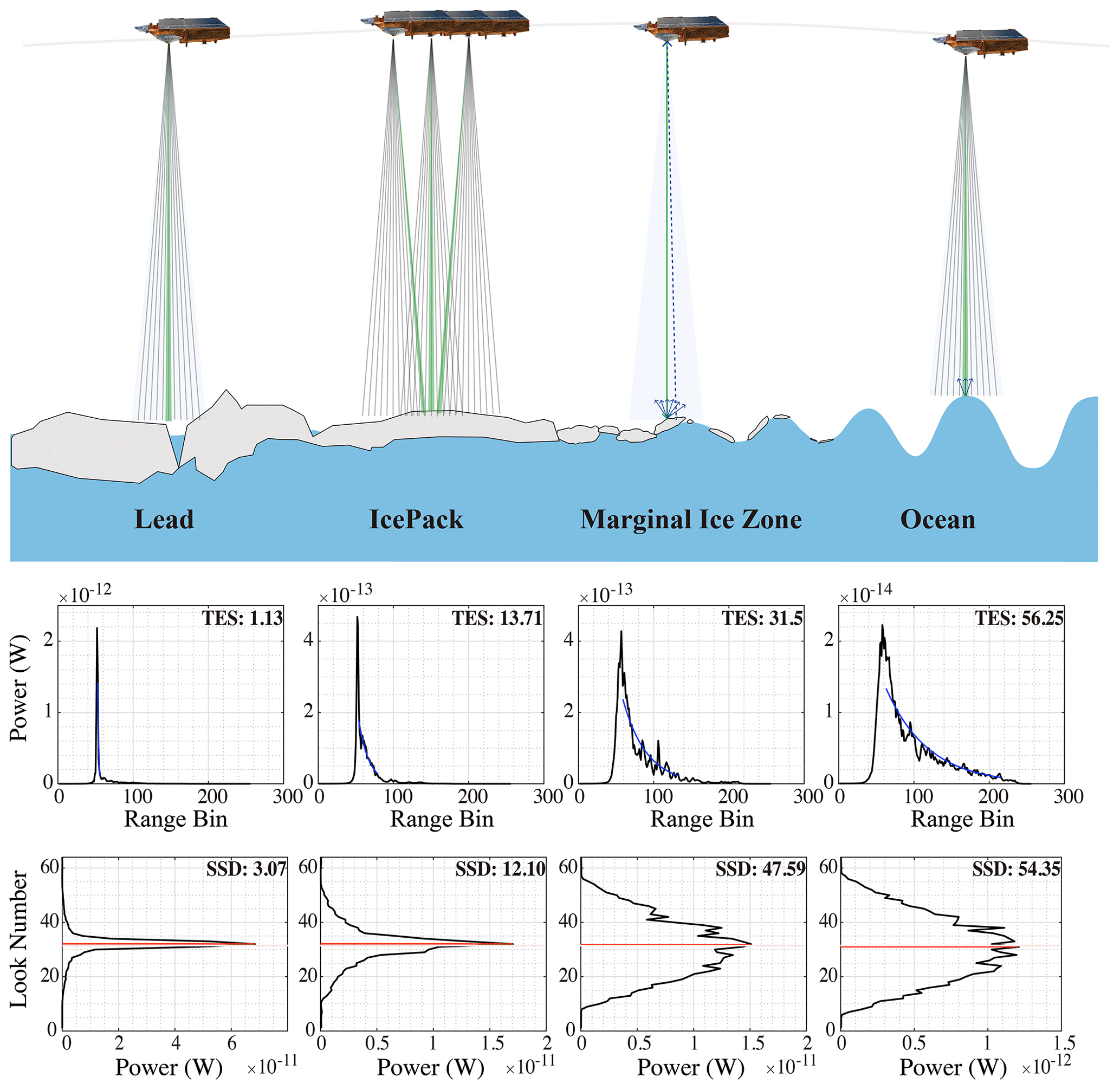
Figure 1CryoSat-2 (CS2) observation of the polar ocean (top panel). CS2 SAR mode waveforms are shown for the four typical surface types in lower panels, including open ocean (right column), wave-affected marginal ice zone (MIZ, second to the right), ice floe (second to the left), and sea ice lead (left). The waveforms are chosen from the CS2 track in Fig. 4. The multilooked waveforms (second row) are shown with the exponential fitting of the power decay in the trailing edge and the fitted parameter of the trailing edge shape (TES). Correspondingly, the range-integrated power waveform and the waveform stack standard deviation (SSD) are shown in the bottom row.
2.2 Auxiliary input datasets
Daily sea ice concentration (SIC) maps are typically generated with passive microwave imaging payloads, and the continuous observation dates back to October 1987 and constitutes one of the longest records of sea ice. For MIZ studies, in Strong and Rigor (2013), the region with SIC between 15 % and 80 % is used as the proxy for the MIZ. In this research, for the CS2 era, we use the SIC product generated at the University of Bremen, which is primarily based on the payload of Advanced Microwave Scanning Radiometer 2 (AMSR2) and the ARTIST Sea Ice (ASI) algorithm (Spreen et al., 2008). For the study period without AMSR2 data (i.e., before 2012), we use the SIC product hosted at the University of Bremen based on the Special Sensor Microwave Imager/Sounder (SSMIS). By default, the 6.25 km resolution SIC product is used, which is sufficient for various analyses in this study, including determining large-scale sea ice edges and the intercomparison with the MIZ width defined by SIC.
For the atmospheric and wave conditions during the CS2's observations, we rely on the global ERA5 reanalysis product (Hersbach et al., 2023). Specifically, hourly sea-surface pressure fields (0.25° resolution) and the wave spectra (0.5° resolution, defined over regions with SIC <15 %) are used. Although ERA5 does not include an interactive sea ice component, its wave product over the ocean is extensively validated with in situ wave measurements globally (Wang and Wang, 2022). The wave product is also well validated and used in various studies of the MIZ and polar oceans (Vichi et al., 2019; Alberello et al., 2022).
2.3 Other satellites assisting in the MIZ retrieval
2.3.1 Sentinel-1
Sentinel-1 (S1) is a polar-orbiting, C-band (5.4 GHz) Synthetic Aperture Radar (SAR) satellite constellation by the ESA and a part of the Copernicus program. The two satellites, Sentinel-1A (launched in April 2014) and Sentinel-1B (launched in April 2016), primarily work in the dual-polarization (HH and HV) and extra-wide (EW) swath mode in the Arctic region, comprehensively covering the Atlantic Arctic. This study primarily uses the Ground Range Detected (GRD) product of the EW mode. The satellites' swath width is approximately 400 km, with a spatial resolution of 40 m. For preprocessing the images, we apply orbit files, thermal noise correction, radiometric calibrations, and terrain correction and convert the backscatter intensity to decibels (dB) with ESA's Sentinel Application Platform (SNAP).
At 40 m resolution, only waves/swells with long wavelengths are identifiable, potentially limiting the use of EW SAR images to the cases with strong, deep-penetrating waves and wide MIZs (Brouwer et al., 2022; Ardhuin et al., 2017). For comparison, under the wave mode of S1 satellites (5 m resolution), the wave spectra and their components can be studied better (Sutherland and Dumont, 2018; Huang and Li, 2022). We use visual inspection and the spectral analysis method to detect waves in ice with SAR images. Specifically, within the sea-ice-covered region of the SAR image, we identify wave patterns with interleaving bright and dark stripes of the radar backscatter and reasonable wavelengths (Collard et al., 2022). Furthermore, the quantitative spectral analysis is performed on the local parts of the SAR image (30 km window size), and the spectral peak is identified and associated with the wave in sea ice. In Appendix B, we introduce the method in detail, and SAR images that collocate with CS2 tracks are used for the analysis and the validation of the CS2-based retrieval in Sect. 4.2 and the Supplement.
2.3.2 ICESat2 and the CRYO2ICE campaign
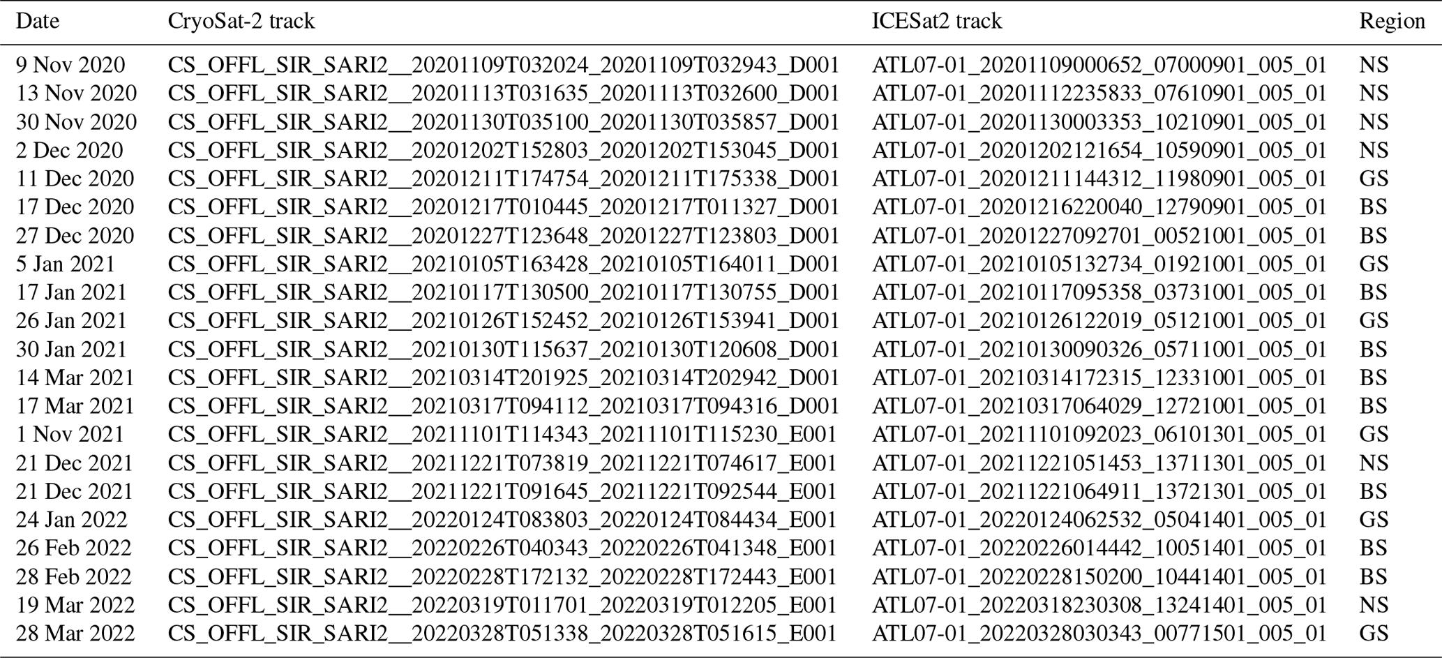
NASA's ICESat2 (IS2) is a photon-counting laser altimeter, launched in the fall of 2018 (Markus et al., 2017). Over sea ice, the laser altimeter primarily measures the range and height of the snow surface, whereas the Ku-band radar signals of CS2 penetrate a significant part of the snow cover. To better evaluate the synergy of the two altimeters for improved snow and ice thickness retrievals (Bagnardi et al., 2021), the CS2 orbit was raised in July 2020 to attain collocated tracks with IS2. Consequently, the ground track of CS2 coincides with that of IS2 at an interval of 19 orbits (about 30 h), and the average visit interval of the two satellites is within 3 h (ESA, 2024a). These collocated tracks are available through the CRYO2ICE campaign (http://www.cs2eo.org, last access: 11 May 2024). In the Atlantic Arctic, we attain 21 collocated track pairs between CS2 and IS2 during the winters (November to April) of 2020–2021 and 2021–2022 (track information in Appendix A).
On sea ice, the nominal spatial resolution of the beam segments of the ATL07 product for IS2 strong beams (SBs) is approximately 17 m (cross-track) and less than 20 m (along-track). Therefore, IS2 can resolve the long-wavelength swells in the sea ice and identify the MIZ. Specifically, in this study, we apply the MIZ retrieval algorithm in Horvat et al. (2020) to the collocated track pairs and compare the result with that based on CS2.
3.1 Retrieval algorithm
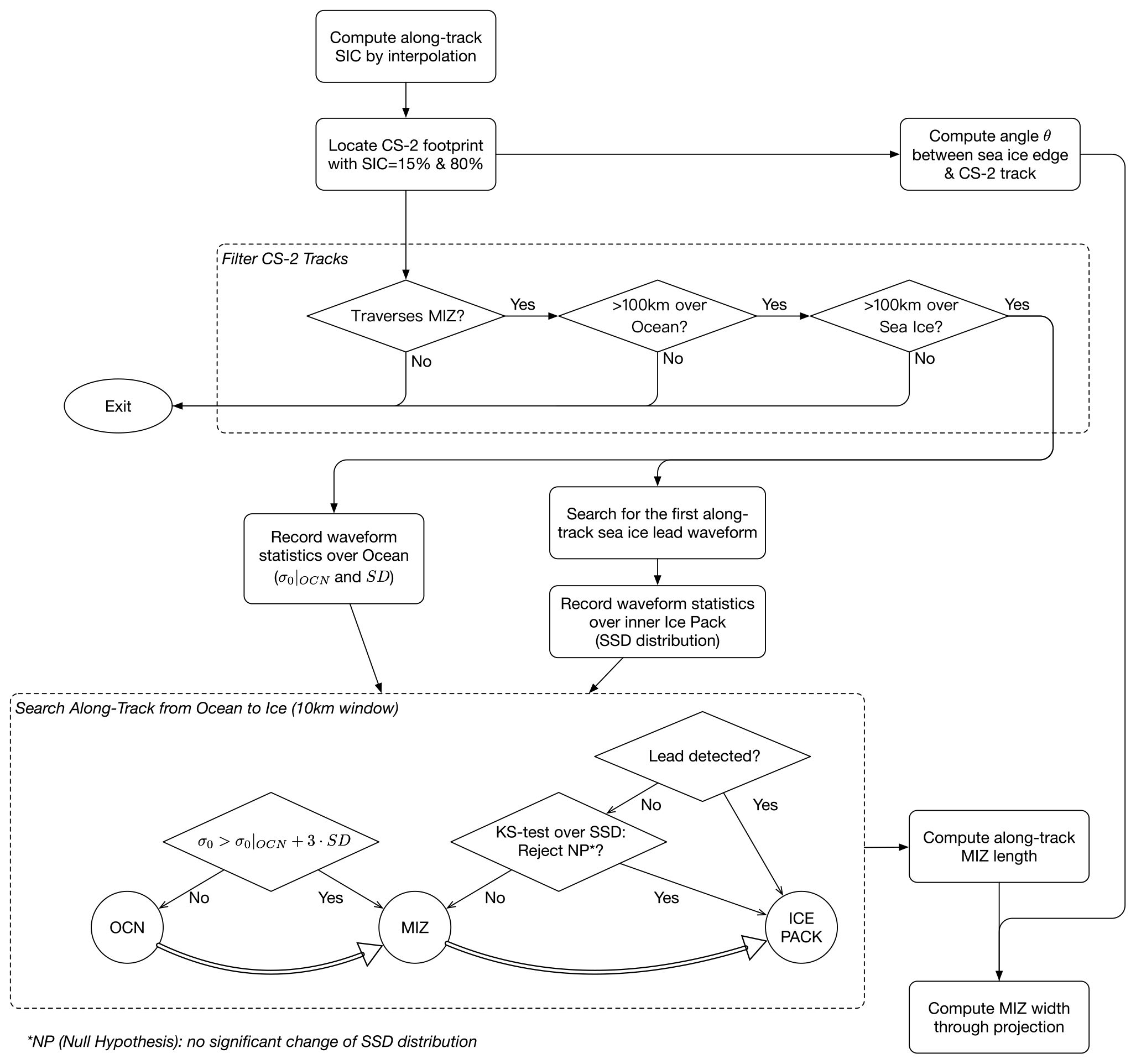
Based on the CS2 waveform properties in the polar ocean, we design the following MIZ retrieval algorithm in Fig. 2. The algorithm primarily uses two parameters: backscatter (σ0) and SSD. First, we detect the beginning of the MIZ with σ0 through its contrast between the ocean and the sea ice. In particular, we use the in situ σ0 over the ocean and its variability (i.e., the standard deviation of σ0, denoted as SD) to account for the variant ocean conditions. When the backscatter is anomalously high (i.e., exceeding 3 ⋅ SD), we detect sea ice and mark the location as the outer boundary of the MIZ.
Second, among the various waveform parameters, we adopt the SSD as an indicator to determine the along-track transition from the wave-affected part (i.e., the MIZ) to the inner ice pack. We conducted statistical tests with the distributions of SSD to determine the inner boundary of the MIZ. Specifically, we search for the first lead waveform (available from ESA's baseline product) in the along-track direction and record the sample-based distribution of SSD from the location of the sea ice lead to 100 km in length (containing over 300 CS2 footprints). Here, the lead is a flat surface with a high speckle return, observed by CS2. Thus, the wave-affected MIZ cannot extend beyond the location of the first lead. Then, the recorded SSD distribution is used as the benchmark to further determine the MIZ's inner boundary.
Third, we restart the along-track search from the MIZ's outer boundary. At each step, we advance into the sea ice direction and record the SSD distribution around the search point. A statistical test is performed to compare the current SSD distribution and that of the inner part of the ice pack. Specifically, the Kolmogorov–Smirnov test (KS test) is adopted to compare the two sample-based distributions. The null hypothesis (NP) is that the two sets of SSD samples follow the same distribution, and it is rejected at the prescribed significance level of 0.05. For determining the inner boundary of the MIZ, we stop the along-track search until (1) the NP of the KS test is not rejected, indicating that the SSD distribution at the current location is consistent with that of the inner ice pack, or (2) the lead previously recorded is encountered.
The SSD distribution of the local part of the track is based on a prescribed window size of 10 km, containing over 30 CS2 footprints. More local SSD samples are included for larger window sizes, reducing the potential of Type-II errors (i.e., premature termination of the search process and underestimating the MIZ length/width). However, larger window sizes inevitably compromise the spatial resolution of the retrieval. Section 3.4 contains the sensitivity study of the window size and the trade-offs.
In the bottom row of Fig. 1 and the typical retrieval scenarios in Figs. 3 and 4, we show the fitted value of TES from the multilook waveform and the SSD. SSD is the standard deviation of the range-integrated power waveform, with larger values corresponding to slower power decay of the increase in the incidence angle.
Coincidentally, higher TES indicates the slower decay of waveform power regarding the gate (or time), promoted by larger height variability and more effective volume scattering typical to the wave-modulated surfaces. For comparison, the retrieval algorithm, as proposed in Rapley (1984), with the pulse-limited altimeter on SEASAT, is based on the (along-track smoothed) significant wave height (SWH), which primarily relies on the leading edge of the waveform. In this study, we choose SSD over TES (or other parameters) due to the larger contrast of the SSD between MIZ and the ice pack (regarding their respective variabilities). To summarize, the proposed algorithm based on SSD has the following advantages: (1) the multi-look capability of CS2 over traditional pulse-limited altimeters, (2) the much enhanced along-track resolution of approximately 400 m with delay-Doppler treatments, and (3) the higher sensitivity for MIZ retrieval with SSD than TES or other waveform parameters. Other retrieval options for historical and future radar altimetry campaigns are discussed in Sect. 6.
Fourth, after the inner and outer boundaries of the MIZ are determined, we compute the along-track length of the MIZ and the MIZ width by projecting it onto the normal direction of the local sea ice edge. Determining the projection angle is based on the sea ice concentration (SIC) maps and introduced below. The projection process is introduced to accommodate the sampling of the CS2 satellite because arbitrary intersection angles exist on its ground tracks and the local sea ice edge in the Atlantic Arctic region.
3.2 Projection and computation of MIZ width
To determine the intersection angle of the CS2 ground track and the local sea ice edge, we need two directions: (1) the ground track's direction, which is readily available from the CS2 product, and (2) that of the local sea ice edge, denoted as ξ. For each MIZ-traversing CS2 track, the daily SIC map corresponding to the CS2's visit time is used to determine the value of ξ. Specifically, we first attain all locations with SIC > 15 % adjacent (i.e., within 100 km) to the ground track's entry point into the ice pack. Second, we scan the range of the potential values of ξ (from 0 to π, relative to the east). For each possible value of ξ, we constructed a local intersection line that separated the aforementioned local area into two parts and computed the accumulated sea ice extent (SIE) for both sides of the intersection line. Then, we defined the final ξ as the angle under which the SIE difference of the two sides is maximum. The method above, including its parameters, is designed to accommodate (1) the inherent fractal characteristics of the sea ice edge and (2) the resolution limitation of the SIC product.
With ξ and the CS2 track direction, we compute the angle of θ, which is the intersection angle for the projection. The width of the MIZ, WMIZ-CS2, is computed as , where LMIZ-CS2 is the along-track length of the MIZ retrieved from CS2. The value θ in the Atlantic Arctic region is typically larger than 45° (Fig. S1) due to the high inclination angle of CS2's orbit at 92°. However, in the Greenland Sea, there are 25 % cases with θ smaller than 30°. For smaller values of θ, the projection process will incur higher uncertainty in the MIZ width, as further discussed in Sect. 3.4.
3.3 Typical scenarios
We investigate two typical scenarios of MIZ retrieval with CS2. On 14 February 2015 (Fig. 3), a CS2 track traversed the sea ice edge in the Barents Sea, and no storm was present in the study region. The normal direction to the local sea ice edge is almost meridional. As indicated by the ERA5 reanalysis (Hersbach et al., 2023), the total (swell) SWH is approximately 1.7 m (1.15 m) near the sea ice edge. Based on the daily SIC map (6.25 km resolution, produced at the University of Bremen with AMSR2), we compute the along-track locations with SIC between 15 % and 80 %. By projecting onto the normal direction of the local sea ice edge, we compute the SIC-based MIZ width of approximately 20 km.
The waveform power measured by CS2 increases from the ocean to the sea ice at about 76.58° N, which is considered the starting location of the MIZ. While TES remained stable over the ocean (55±3), it showed (1) much larger variability on the sea ice and (2) an overall decrease toward the inner part of the ice pack. The smaller TES on sea ice indicates a stronger waveform peak and much faster waveform power decay regarding time (or gate number). Consistent with the changes in TES, the value of SSD also decreased from over 50 looks on the ocean to fewer than 20 looks on the inner ice pack, indicating stronger central looks than slant-looking ones in the ice pack. A slight shift in the stack center angle is also present due to the gradual decrease in surface height to the north.
For comparison, in Fig. 4, we show the case on 17 February 2015, with a heavy storm passing around Svalbard (3 d later than the case in Fig. 3). The same storm event is also recorded during the in situ campaign of N-ICE2015 (denoted as M3 in Graham et al., 2019). The total SWH is over 3.9 m, with the swell power accounting for over 94 % of the total power. The CS2 track entered the sea ice cover at 76.6° N, and the waveform parameters gradually transitioned over a long distance to the relatively calm ice pack in the north. Within the MIZ, the SSD and TES gradually decrease and show a larger spatial variability than the ocean and the inner part of the ice pack. The sharp contrast of waveforms in the MIZ to those on the ocean or the inner ice pack is also evident in the overall waveform profile (bottom panel of Fig. 4). Based on SSD and the retrieval algorithm in Sect. 3.1, we determine that the along-track MIZ terminates at approximately 79.1° N. The retrieved along-track MIZ length is over 270 km (yellow shading in Fig. 4). The CS2-observed MIZ length is much larger than that based on along-track SIC (purple shading), which is only 35 km.
The nearest available SAR image from S1 (EW swath mode, 40 m resolution) is 3.1 h after CS2's observation (Fig. 5). The time difference is within the typical temporal scale of MIZs of 6 h; hence there is good collocation between the two satellites (Brouwer et al., 2022). Swells in the ice pack are evident from the SAR image, with the apparent wavelength of approximately 400 m. Based on the SAR images, the outstanding peak of the spectrum of the local backscatter map identifies MIZ, with a consistent wavelength estimation (i.e., Fig. 5d and e). The intersection angle of the dominant swell propagation direction and CS2 ground track is approximately 47°. As shown in Fig. 5c, the spectral peak corresponding to the wave structure diminishes to the north of the retrieved MIZ. The CS2-retrieved MIZ termination location deviates from that based on the spectral analysis by less than 10 km (4 % of the along-track MIZ length). Given the 3 h difference between the two satellites' visit times, we consider that the CS2 retrieval of the wave-affected MIZ is consistent with that based on the SAR images.
Interestingly, the stack center angle of CS2 shows an oscillatory pattern toward the northern end of the MIZ at 79° N (Fig. 4d). The central look (with a Gaussian fitting) deviates from the nominal location by 1600 m from the nadir location in the along-track direction. A similar phenomenon is witnessed for many stormy events (another example in Fig. 6). The apparent wavelength of this oscillatory pattern is of the order of kilometers, much larger than the swell wavelength (Fig. 5). According to the CS2 dataset, the aircraft yawing and/or pitching is not the primary cause. We conjecture it an aliasing effect caused by long-wavelength swells and the misalignment of their propagation direction to the CS2 track.
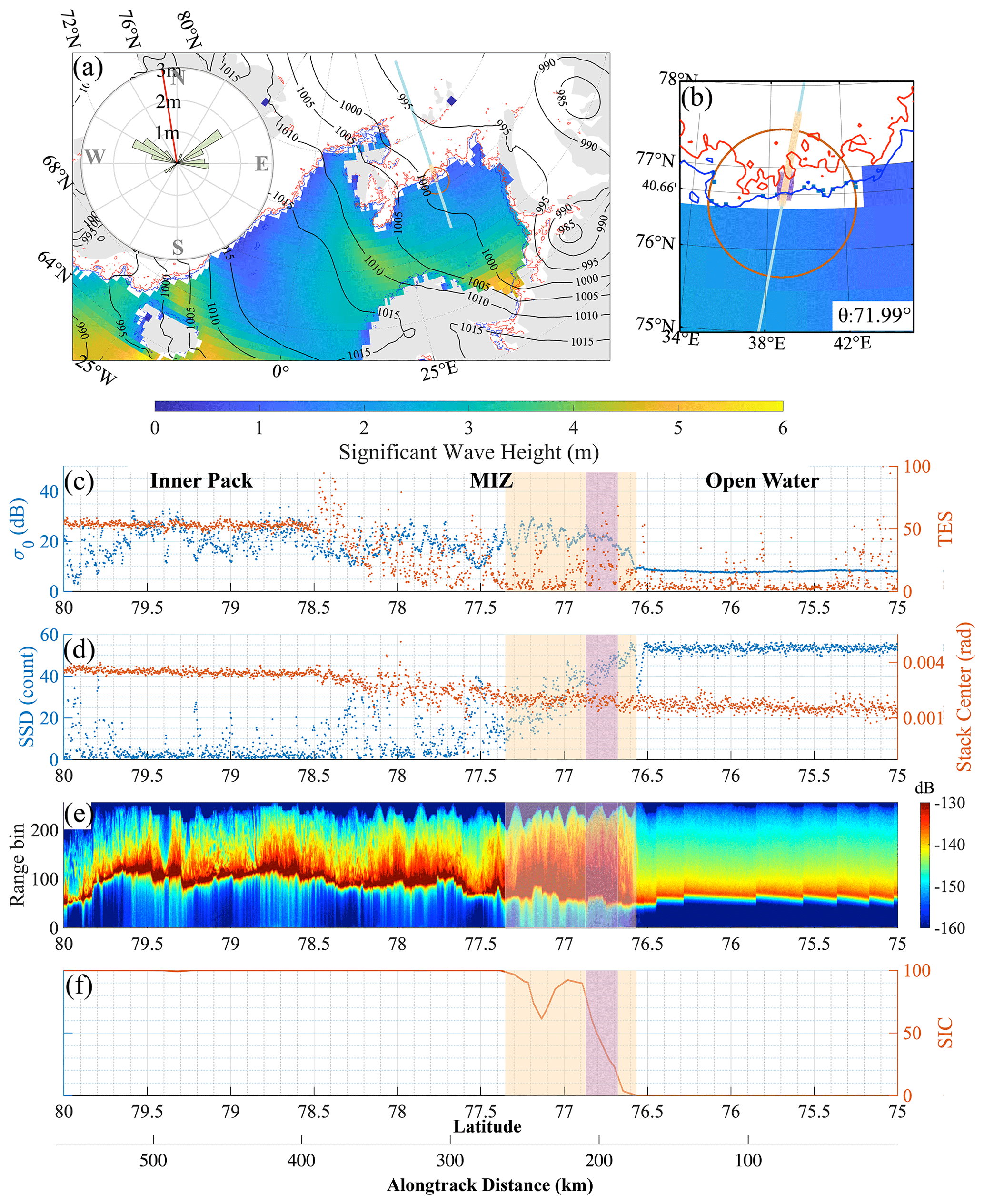
Figure 3CS2 observation of the MIZ in the Barents Sea on 14 February 2015 (at 00:06 UTC). In the top panels (a, b), the hourly total SWH (filled contour) and sea-level pressure (labeled contour lines) are both derived from ERA5 data. The SICs of 15 % and 80 % are represented by blue and red contour lines, respectively. The CS2 track is shown by the thin light blue line, with the SIC-based (or CS2-retrieved) MIZ highlighted by thick purple (or yellow) line. The inset rose map shows the swell power and direction spectra near the entry point of the CS2 track into the ice pack (within the circle in panel b), as well as the normal direction into the sea ice edge (red line, details in Sect. 3.2). Additionally, the intersection angle (θ) between the sea ice edge and the CS2 track is shown in the zoomed-in view of panel (b). Along-track CS2 waveform and waveform stack parameters are shown in lower panels, including (1) backscatter (σ0) and TES in panel (c), (2) SSD and stack center angle in panel (d), (3) the waveform power in panel (e), and (4) the along-track SIC in panel (e). In lower panels (c–f), the MIZs retrieved with SIC and CS2 are also marked with the same colors as in the top panels.
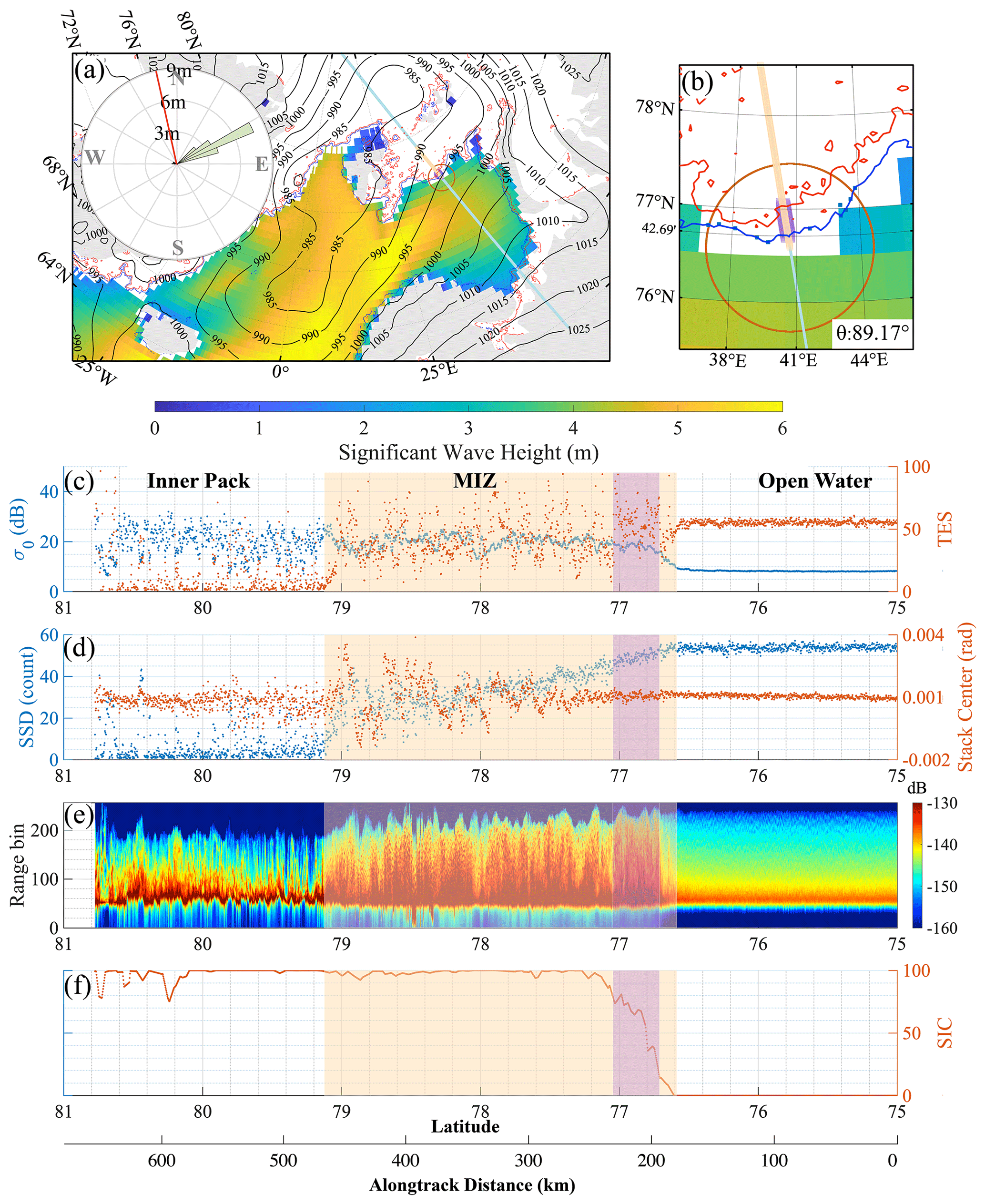
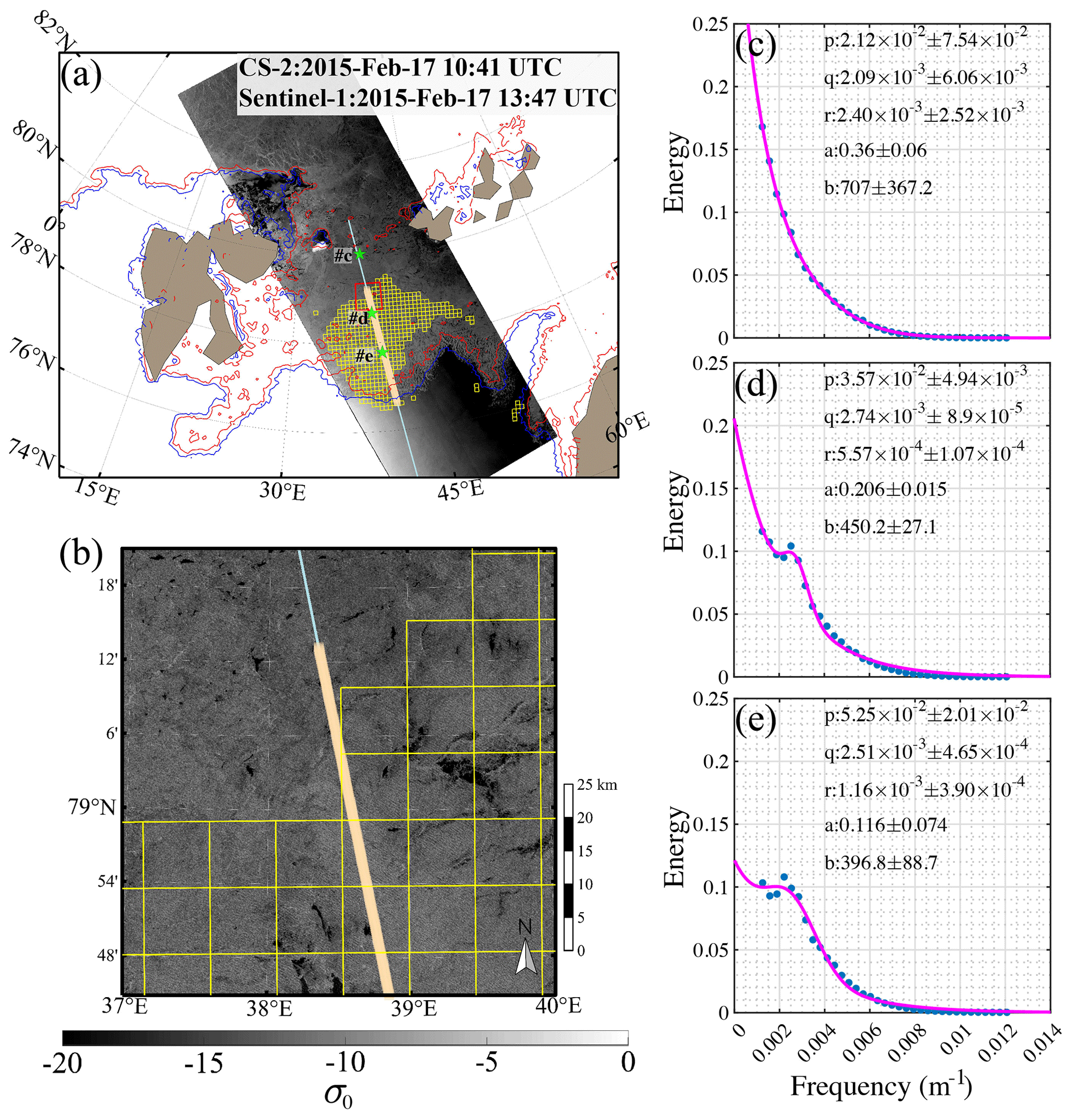
Figure 5Collocated SAR images from Sentinel-1 (EW mode, panel a) for the MIZ in Fig. 4 and the northern end (red box in panel a) of the CS2-retrieved MIZ shown in detail (panel b). The region with detected wave in ice by spectral analysis (Appendix B) on the SAR image is marked by yellow boxes (10 km scale). The spectra of the Sentinel-1 backscatter map of three typical regions (green dots in panel (a) and in panels (c)–(e) corresponding to the northernmost, the middle, and the southernmost) are shown on the right, along with the respective fitted parameters and their uncertainties in Eq. (B1).
3.4 Sensitivity of retrieval to algorithm parameters
We consider the uncertainty of the retrieval caused by two crucial parameters: (1) the window size for accumulating the statistics of SSD and (2) the intersection angle of θ for the projection. We first evaluate the effect of window size on the retrieved lengths of the MIZ in the along-track direction. Besides the default window size of 10 km, we assess two extra window sizes: 5 km (or 15 CS2 footprints) and 20 km (or 60 CS2 footprints). With larger window sizes, we generally attain larger values of the MIZ width (Fig. S2). Since more SSD samples are available with larger windows, the false rejection of the null hypothesis is reduced during the KS test (Fig. 2), resulting in wider MIZs. However, the retrieval results with 10 and 20 km window sizes are highly consistent, with the correlation coefficient at 0.99, the fitting slope at 1, and only 1 km difference in the MIZ length. Also, at larger window sizes, the spatial resolution of the retrieved MIZ is potentially compromised. Therefore, we choose the window size of 10 km by default for all retrieval studies.
We also estimate the relative uncertainty in the MIZ width incurred by that in θ. The uncertainty of θ originates from the sea ice concentration map around the entrance of the CS2's ground track into the ice edge. Through perturbation analysis, we estimate that the uncertainty, denoted as Δθ, is on average 6.5° in the Atlantic Arctic region. The relative uncertainty of LMIZ due to θ, under the small-angle assumptions, is then computed as
Among all the tracks, most θ is larger than 30° (e.g., Fig. S1), and the relative uncertainty is lower than 20 %. Furthermore, to ensure 10 % or lower relative uncertainty, the value of θ should be larger than 45°. For the BS, the NS, and the GS region, 88 %, 82 %, and 37 % tracks satisfy this criterion, respectively. For satellites with different orbit inclination angles than CS2, the distribution of θ differs and is potentially complementary to that of CS2, especially in the GS region.
We validated the MIZ retrieval based on CS2 by conducting a comparative analysis with that derived from the IS2 laser altimeters and the SAR imagery from S1. IS2 and S1 attain high-resolution sampling of the sea ice cover and the MIZ. However, the MIZ retrieval with IS2 is based on its capability to resolve the height signature of waves in the MIZ, whereas that with S1 relies on the wave-modulated backscatter. These methods differ from the proposed CS2-based retrieval methods; hence, they also provide us with complementary perspectives of the processes in the MIZ.
4.1 Validation with ICESat2 from CRYO2ICE campaign
We compare the along-track MIZ lengths retrieved with the two satellites based on the collocated tracks between CS2 and IS2 from the CRYO2ICE program (Bagnardi et al., 2021). We limit the analysis to the track pairs with the distance between the ground tracks less than 50 km, eliminating the track pairs without actual collocation in the Atlantic Arctic region. Besides, given the highly variant conditions of MIZ, we only study the track pairs with observation time differences of less than 3 h. Finally, we attain 21 track pairs in the Atlantic Arctic for the two winters of 2020–2021 and 2021–2022 (track information in Table A1). For each track pair, we retrieve the MIZ's boundaries with HC20 and the strong beams (SBs) in the ATL07 dataset of IS2 (release 5).
In Fig. 6, we show an example of MIZ affected by a storm in the Barents Sea, observed by a pair of collocated tracks of CS2 and IS2. The two satellites' visit time is separated by 3 h. Strong swells (swell SWH = 1.95 m and the total SWH = 2.62 m) propagated into the ice pack, with the CS2-observed MIZ length of over 170 km. Different from the case in Fig. 4, the SIC-based MIZ is comparable to that based on CS2, primarily due to a wide and loose ice edge. For IS2, the MIZ observation relies on the high-resolution, high-precision elevation measurements over sea ice, allowing for the direct sampling of waves with relatively long wavelengths (Horvat et al., 2020; Brouwer et al., 2022). The surface elevation measurement in the ATL07 product of IS2 only contains valid photon segments over sea ice (i.e., no data on the ocean; last panel in Fig. 6). The large oscillatory, wave-like structure of the surface elevation (i.e., periodic signals with amplitudes over 50 cm) is evident, indicating the wave-affected MIZ. The gradual decrease in the wave amplitude toward the north implies the wave attenuation within the MIZ. We retrieved the northern end of the MIZ with the algorithm proposed in Horvat et al. (2020) (denoted by HC20 hereinafter). The location of the MIZ's northern boundary as retrieved by IS2 is offset from the CS2 retrieval by only approximately 1 km (<1 % of the total MIZ length). Since the ATL07 product only includes valid measurements on sea ice, we treat the south-most photon segment with a valid elevation in ATL07 as the MIZ's southern end observed by IS2. It is worth noting that, for this specific case, the photon segments are not continuous near the MIZ's southern end, probably due to (1) the cloud contamination and/or (2) the relatively fine footprints of IS2. In general, we consider the CS2 and the IS2 retrieval of MIZ consistent, especially given the fast-changing nature of MIZ and the 3 h difference in visit times.
Similar to the case in Figs. 4 and 5, we performed spectral analysis of the case in Fig. 6 (the results are shown in Fig. S8). The visit time of S1 is approximately 2.5 h ahead of IS2 and 5.5 h ahead of CS2. The apparent wave structure on the SAR image covers over 150 km into the ice pack and terminates at 78° N, well captured by the spectral analysis. The location of wave's presence in the sea ice is highly consistent among the three satellites (all within 10 km).
Using all 21 collocated tracks from the CRYO2ICE campaign, we compare the location of the retrieved MIZs from CS2 and IS2 (the nearest SB to the respective CS2 track). The MIZs' southern and northern boundaries are shown in Fig. 7 (left and middle panels, respectively). Specifically, we compare the latitudes of the boundaries because these tracks are almost meridional in this region. As shown, very high statistical correlations (Pearson's r over 0.99) are attained for the southern and northern boundaries of the MIZs. Furthermore, for the along-track MIZ length (the right panel of Fig. 7), the retrievals with CS2 and IS2 are also highly consistent (r=0.86). The linear regression between CS2 and IS2 yields a fitting slope of 0.87±0.25, indicating no systematic difference. Besides, the correlation is higher in the Barents Sea than in Greenland Sea, which may be due to a more mobile and spatially noncontinuous sea ice cover in the latter. The along-track MIZ length is in the range of 5 and 180 km, indicating that various MIZ conditions are covered, including calm cases and stormy ones associated with wide MIZs (e.g., Fig. 6).
It is worth noting that MIZ retrievals with CS2 and IS2 are based on different approaches. For IS2, the retrieval relies on directly observing wave structures through the high-resolution sampling of photon segments. Rather than directly resolving the waves, the retrieval with CS2 is primarily based on the aggregate behavior of radar waveforms over the wave-modulated sea ice cover. One common characteristic of CS2- and IS2-based MIZ retrieval is that the spatial representation of the altimeter is inherently limited. Related issues, including quantifying representation uncertainty, are further discussed in Sect. 6.
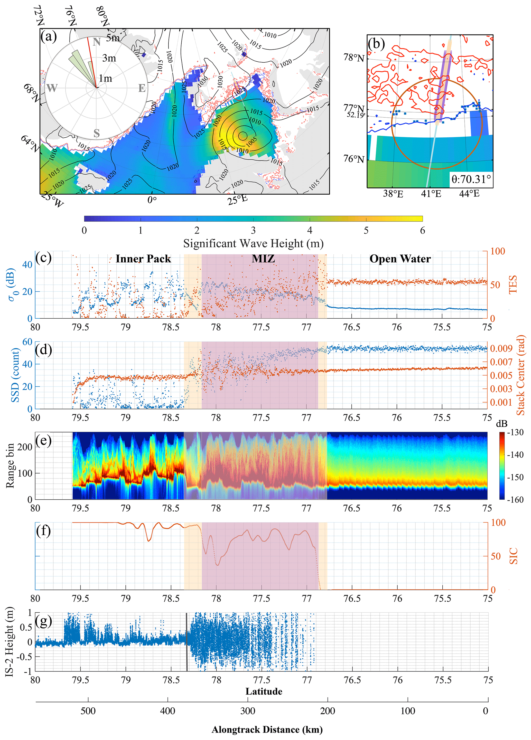
Figure 6CS2 and IS observation of the MIZ in the Barents Sea on 17 March 2021. Similar to Fig. 4, strong swells propagate into the ice pack, with the MIZ width over 170 km. The MIZ is sampled by a pair of collocated tracks by CS2 (at 09:40 UTC) and IS2 (at 06:40 UTC), with the time difference of 3 h. The additional panel, panel (g), shows the along-track IS2 elevation, as well as the retrieved northern boundary of the MIZ with HC20 (vertical black line around 78.4° N).
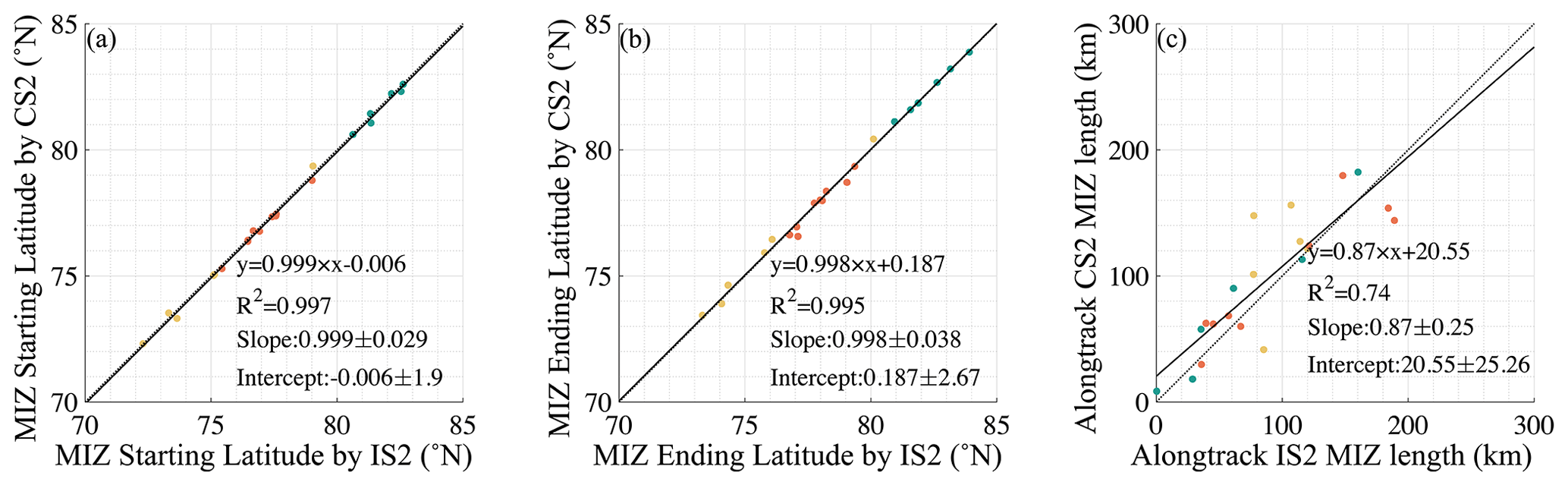
Figure 7Comparison of along-track MIZ retrievals with collocated tracks of CS2 and IS2 in the Atlantic Arctic during the winters of 2020–2021 and 2021–2022. Each dot represents a track pair, with 21 pairs in total. The dots are color-coded according to the track locations: orange for those in the Barents Sea, yellow for those in the Greenland Sea, and green for other tracks around Svalbard. The representation ranges of these locations are the same as Fig. 8. The comparison of the along-track MIZ starting and stopping latitudes is shown (left and middle panels, respectively) with that for along-track MIZ lengths (right panel). The linear regression line (solid black) and the fitting parameters are shown in each panel, together with the 1:1 line (dotted black).
4.2 Analysis with collocating S1 images
Based on the 21 collocated tracks from the CRYO2ICE campaign, we further find available collocating S1 images (EW mode). We ensure temporal collocation by limiting the observation time of the S1 satellites to be within 6 h of that by CS2. There are nine cases with the collocated observation of all three satellites (an example is in Fig. 6). We perform visual inspection and spectral analysis for all the SAR images, and the results are listed in Table 1 and Figs. S3 to S11.
Six of the nine cases show evident wave penetration in the sea ice cover. The spectral analysis successfully identifies four out of the six cases, consistent with the retrieval results by CS2, IS2, and S1 (cases no. 2, no. 3, no. 4, and no. 6). Case no. 5 (Fig. S7) features an inhomogeneous ice edge and a mixture of ice floes and open water. Although the visual inspection reveals evident wave structures over the ice-covered region, the spectral analysis fails to detect outstanding peaks in the spectrum. Also, for case no. 9 (Fig. S11), the MIZ detected by CS2 is further north of the IS2 retrieval and the spectral analysis based on the S1 image.
For the other four cases without waves detected by visual inspection or spectral analysis, the dominating processes are from the ocean. For example, for case no. 1, the frazil streaks are governed by new ice formation, and Langmuir circulation forms the MIZ. CS2 and IS2 successfully identify it. For the ocean-turbulence-dominated ice edges (i.e., cases no. 4, no. 7, and no. 8), the regions with sea ice free drift are also correctly retrieved by both altimeters. The reason that spectral analysis fails to identify waves for these cases may be the coarse resolution of the S1 EW image (40 m resolution) and the complex, inhomogeneous ice edge.
Table 1Analysis of the collocated observation by Sentinel-1 with the track pairs from the CRYO2ICE campaign. The type of the ice edge in each case is determined by visual analysis of the Sentinel-1 image.
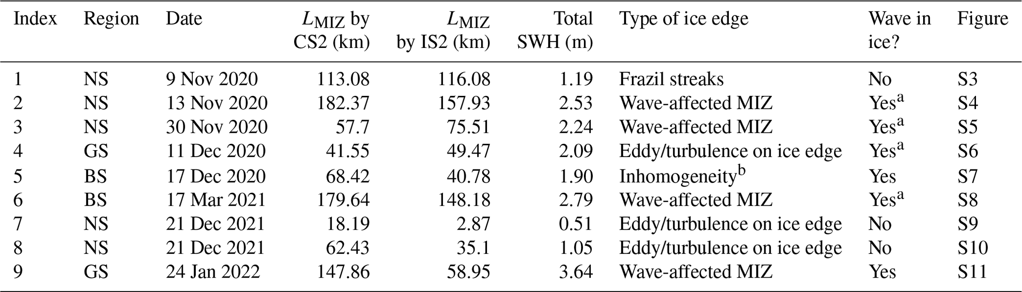
a Wave in ice detected by spectral analysis on the backscatter map of S1 EW image (see Appendix B). b Inhomogeneous ice edge with the mixture of ice floes and open water, with waves only visible on ice patches.
Based on the retrieval for the wintertime CS2 observations, this section reports the climate record of MIZ in the Atlantic Arctic region for 2010–2022. We divide the Atlantic Arctic into three subregions: the Barents Sea (BS; south of 80° N and east of 15° E), the north and northwest of Svalbard (NS; region east of 0° E except BS), and the Greenland Sea (GS; 30 to 0° W). There are 2818, 3007, and 3160 valid CS2 tracks for BS, NS, and GS, respectively. Temporally, we investigate the whole winter and the two periods of the winter: the first half from November to January and the second half from February to April. In Sect. 5.1, we report the basic statistics of the retrieved MIZ width and in Sect. 5.2 its interannual variability and the study of typical winters. Finally, in Sect. 5.3, we compare the CS2-based retrieval with the traditional definition of MIZ based on SIC.
5.1 Statistics of MIZ widths
In Table 2, we show the general statistics of the MIZ width (i.e., WMIZ) of all 12 winters and in Fig. 8 for every 3 months. MIZ width follows a skewed distribution in all regions, with the mean width of 78.55, 41.03, and 55.98 km for BS, NS, and GS, respectively. The modal MIZ widths, representative of the typical, non-stormy conditions, are 32.04 km (BS), 11.20 km (NS), and 39.53 km (GS). Correspondingly, the distribution of WMIZ is highly skewed, and the cases of wide MIZs are associated with storm events (Figs. 4 and 6).
Among the three regions, the widest MIZs manifest in BS, with the largest width reaching over 250 km in most winters. Also, within each winter in the BS region, the MIZ width decreases in the later stage. This phenomenon is not observed for the other two regions. The potential reason might be ice thickening as the winter progresses, which is more evident in BS.
In NS, the MIZ is generally narrower than in BS and GS. For certain years, such as 2014–2015, the sea ice edge is only present to the west of Svalbard (i.e., no ice edge north of Svalbard). Sea ice in NS originates from within the Arctic Ocean due to the ice advection through the transpolar drift and the interaction with the Atlantic inflow. It is typically older and thicker than the locally grown sea ice during the freeze-up season. Consequently, the swell penetration into the ice pack is potentially limited due to the higher ice thickness, and the MIZ is generally narrower in NS.
Among the three regions, GS shows the overall largest modal MIZ widths. However, the mean MIZ width is smaller in GS than BS, primarily due to the extremely wide MIZs, which are more common in BS. Coincidentally, the skewness of the MIZ width distribution is also the lowest in GS. This result is due to the generally loose ice pack in the GS resulting from the south-bound, fast ice drift and divergence.
During 2010–2022, we do not observe statistically significant changes in the wintertime MIZ width. Similarly, no significant changes occur in extreme cases of MIZ width (i.e., top 5 %) for the three regions of the Atlantic Arctic. For comparison, no significant changes in SIC-based MIZ width are observed for the same period (2010–2022), although it is generally much lower than the CS2-based retrieval.
Table 2Statistics of wintertime MIZ width based on CS2 and the along-track SIC from 2010 to 2022.
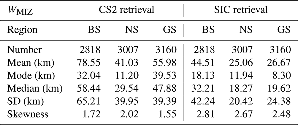
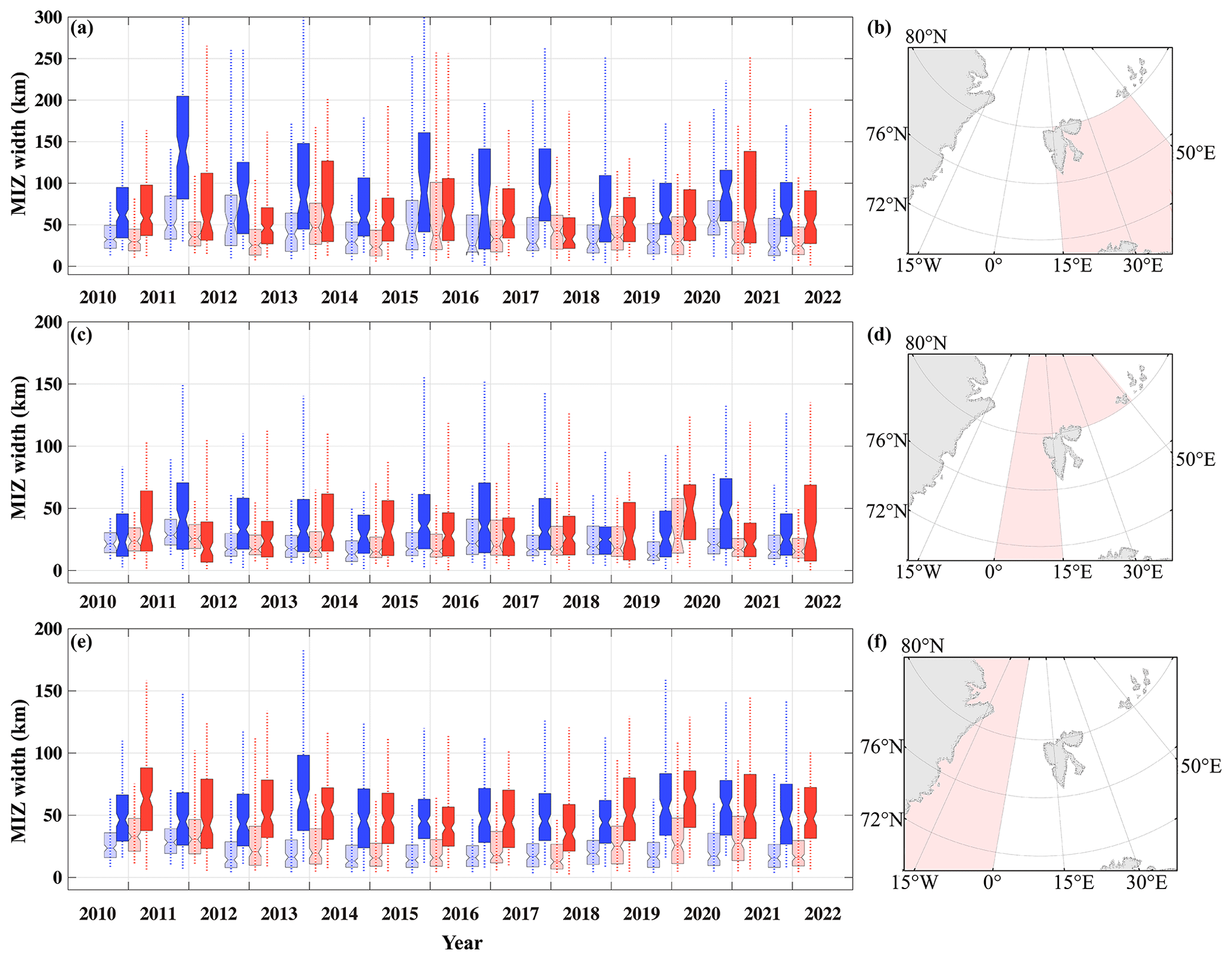
Figure 8Statistics of wintertime MIZ width from 2010 to 2022. Two 3-month periods of each winter (November–January in blue and February–April in red) are shown for the Barents Sea (BS; a, b), the north/northwest of Svalbard (NS; c, d), and the Greenland Sea (GS; e, f), separately. The median, the inter-quantiles (box), and the 5th and the 95th percentiles (vertical line) of MIZ width distribution are shown. Statistics of SIC-based MIZ width on the same CS2 tracks are shown in lighter colors.
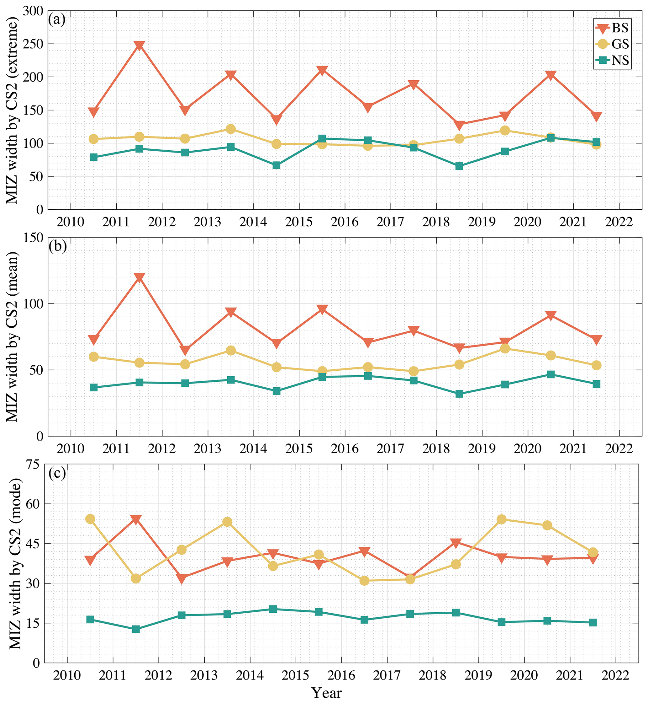
Figure 9The extreme (a), the mean (b), and the modal MIZ widths (c, in km) of each winter from 2010 to 2022. Specifically, the extreme MIZ width is computed as the mean MIZ width of the widest 10 % MIZs of each winter. Note the difference in the MIZ width ranges (from 300 km in panel a to 75 km in panel c).
5.2 Interannual variability and typical winters
Although no change in MIZ width is detected, a large temporal variability exists, both interannually and intraseasonally. In particular, in Fig. 9, we show a pronounced interannual variability (IAV; 2-year cycle) of the extreme MIZ widths (top 10 %) in the Barents Sea. For comparison, the modal width in the Barents Sea (e.g., non-stormy condition) does not show similar variability. Collaterally, the mean width shows similarly pronounced IAVs caused by the cases with extremely large widths.
Various factors cause the extremely wide MIZs, including strong storm events and relatively thinner/looser ice edges. In the Barents Sea, the IAV of the widest MIZs coincides with the statistically significant correlation of seasonal mean MIZ widths between the CS2-based retrieval and the retrievals based on SIC (details in Sect. 5.3). For winters with a relatively loosely packed ice edge in the Barents Sea, the SIC-based MIZs are wider, and the ice edge is more susceptible to storms and wave intrusion. However, the quantitative role of these contributing factors, including the IAV of storms and the ice thickness, is beyond the scope of this study and is planned for future work. For comparison, in the other two regions (BS and NS), we have much lower IAV in the extreme MIZ widths than in the Barents Sea.
Due to the large IAV of the MIZ width, we examine two winters for comparison: 2012–2013 and 2014–2015. The results are shown in Fig. 10. The winter of 2012–2013 followed the record minimum of Arctic SIE in September 2012. Besides, it was a relatively calm winter in the Atlantic Arctic, with weak storms throughout the season (Rinke et al., 2017). The sea ice coverage gradually increased in the Barents Sea as the winter progressed from November to January (the top panels of Fig. 10), primarily due to the in situ ice growth, assisted by the advection from the north. Although only weak storm events were present during this period, wave-affected MIZs extended as far as 85° N (i.e., 600 km north of Svalbard). For the latter 3 months of the 2012–2013 winter, the wave-affected MIZ around Svalbard was not as prominent as in the former period, only manifesting in the Barents Sea.
Since the sea ice minimum in September 2012, the Arctic sea ice cover has undergone recovery up to 2015, with larger ice coverage and thicker ice (Tilling et al., 2015). Furthermore, the winter of 2014–2015 witnessed frequent storms in the Atlantic Arctic region (Graham et al., 2019). These characteristics are also reflected in the wave-affected MIZs (the lower panels in Fig. 10). In contrast to the winter of 2012–2013, there was already large ice coverage in the Barents Sea (77° N) from November 2014. The sea ice coverage generally remained high throughout the winter. However, due to frequent storms, the CS2-observed MIZ extends into the ice pack of over 250 km in the Barents Sea and the Greenland Sea. However, given the larger ice coverage and potentially thicker ice than the winter of 2012–2013, we do not observe any MIZ beyond 82.5° N during the winter of 2014–2015.
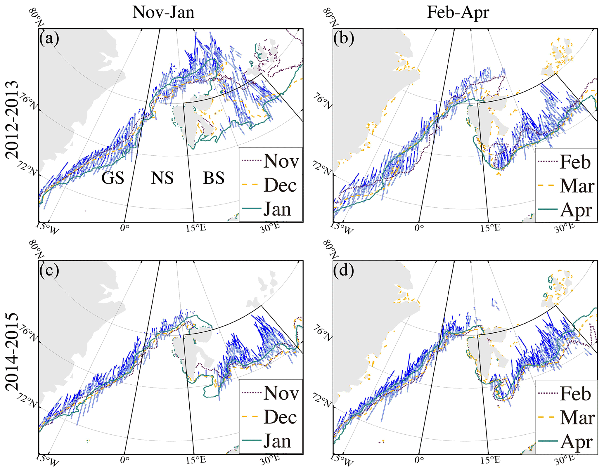
Figure 10Along-track CS2-retrieved MIZ of two typical winters: 2012–2013 (a, b) and 2014–2015 (c, d). The two periods of the winter (November–January and February–April) are shown in the left and right panels, respectively. The monthly mean sea ice edge is shown for each month with contour lines in all panels. For each CS2 track, the part with (daily) along-track SIC lower than 80 % is shown in light blue and that over 80 % in dark blue.
5.3 Comparison with SIC-based MIZ
We systematically compared the CS2-based MIZ width retrieval and the traditional MIZ definition based on SIC (i.e., SIC between 15 % and 80 %, as in Strong and Rigor, 2013). Specifically, two SIC-based MIZ widths are computed. The first method is demonstrated in the examples in Figs. 3, 4, and 6 and is based on the SIC along the CS2 track. For each CS2 track, we attain the along-track SIC and compute the distance between SIC = 15 % and SIC = 80 % as the along-track MIZ length. Then, the MIZ width is computed with the same projection method as in Sect. 3.2. The second method is as follows: for each CS2 track, we compute the MIZ width based on the aggregate area with SIC between 15 % and 80 % in the adjacency of the track (within 100 km of the track). This method is inherently based on box-counting and is free from the potential representation issues with altimetric scans of the MIZ.
Table 2 and Fig. 8 compare the SIC-based retrievals with the first method. As shown, the SIC-based MIZ width also follows a highly skewed distribution. However, the MIZ defined with SIC is narrower than the CS2 retrieval, including the mean and extreme widths. For example, for BS, GS, and NS, the mean width is lower by 43 %, 52 %, and 39 %, respectively. More importantly, there is only a weak statistical correlation between the SIC and the CS2-based MIZ widths (10 % common variance; Fig. 11a).
At larger temporal scales (i.e., 3 months), the mean MIZ width based on SIC correlates with that based on CS2 only in the BS region (with the correlation coefficient r of 0.62 and p value <0.01) but not in the GS or NS regions. For the BS region, the correlation is significant at the monthly and the interannual scales (r=0.57 and r=0.75, respectively, and the p values are lower than 0.05). This statistical relationship might not be due to the inherent physical relationship between the wave-affected MIZ and the daily SIC but the large-scale sea ice conditions, including ice edge advance and ice thickening throughout the winter.
Between the two SIC-based retrievals, an overall consistency exists between the two (R2=0.52, Fig. 11b). The box-counting method yields slightly lower MIZ widths (by approximately 3.5 %), and we consider it a minor issue due to the practical way of computing the area with 15 % < SIC < 80 %. More importantly, the comparison in Fig. 11b reveals the representation uncertainty with altimetric observations of the MIZs. It is worth noting that, similar to the intercomparison between CS2 and IS2 retrievals (Sect. 4.1), temporal and spatial representations should be accounted for during the altimetric observations of the MIZ. The representation issue and the potential with the synergy of multiple altimetry campaigns are further discussed in Sect. 6.
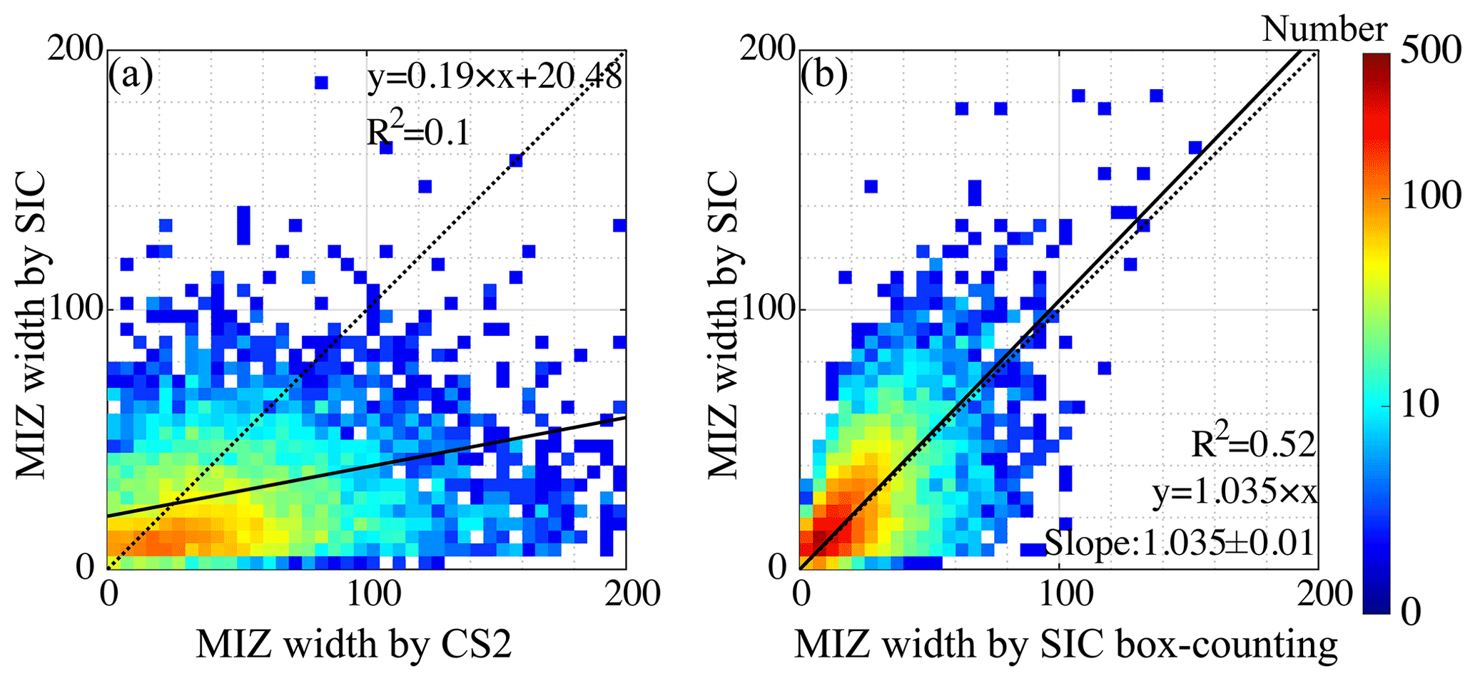
Figure 11Comparison of MIZ width based on CS2 retrieval and the along-track SIC (a), and that of the SIC-based MIZ width retrieved with along-track SIC and the box-counting method (b).
In this study, we design a new retrieval method for the wave-affected marginal ice zones with the radar altimeter of CS2. The waveform and the waveform stack parameters of CS2 are used to retrieve the along-track locations of the MIZs. Based on the available CS2 dataset spanning 2010–2022, we retrieve the winter months in the Atlantic Arctic region. The retrieval is validated with collocated observations of IS2 and S1. The new dataset contains over 8985 MIZ-traversing CS2 tracks and yields good spatial and temporal coverage of the MIZs in the Atlantic Arctic (Zhu et al., 2023).
Based on the new dataset, we investigate the status and potential changes of the wave-affected MIZs in the Atlantic Arctic. No evident change in the mean or largest MIZ widths is detected during 2010–2022, but large spatial (region-to-region) and temporal (e.g., interannual) variability is present. The three regions of the Atlantic Arctic, distinct in their respective sea ice conditions, show drastically different properties of the MIZs. Despite the modal MIZ width of 32 km in the Barents Sea, the wave-affected MIZs can reach over 300 km into the ice pack. In particular, a pronounced, 2-year cycle IAV of the extremely wide MIZs in the Barents Sea exists. The attribution to storms and sea ice conditions is planned for future work. The modal MIZ width in the Greenland Sea is generally the largest, and the width distribution shows the lowest skewness. The region around Svalbard contains the narrowest MIZs due to higher ice concentration and thicker ice. The comparison also indicates that the traditional definition of MIZ based on SIC inherently underestimates the wave-affected MIZ width. More importantly, the (daily) SIC maps do not indicate the wave-affected MIZs (i.e., no statistically significant correlation).
6.1 On the SIC-based MIZ definition
Although the daily SIC maps do not indicate the wave-affected MIZs, there is a statistically significant correlation between the mean MIZ width based on CS2 retrieval and that based on SIC at larger temporal scales. In particular, only in the Barents Sea does the mean MIZ width based on SIC correlate with that based on CS2 retrievals, although the former is much narrower by 43 %. As analyzed in Sect. 5.3, we conjecture this as the result of large-scale sea ice conditions. During many winters, the sea ice edge advance in the Barents Sea ensures large SIC variability on monthly or larger scales. New ice forms during the sea ice edge advance and is more susceptible to wave/swell effects due to the low thickness. Consequently, a more loosely packed and more mobile ice cover forms, coinciding with a wider MIZ.
Given the large sea ice edge changes throughout the winter, if SIC maps at coarser temporal resolutions were used to generate the MIZ maps (same threshold values of 15 % and 80 %), we could attain a wider MIZ from SIC. On the other hand, if the SIC variability (instead of the mean SIC) is used, we also witness a systematic increase in the retrieved MIZ width. We cannot directly resolve the wave's effect on MIZ with either mean SIC or SIC variability. Similarly, Vichi (2022) explored defining MIZ based on SIC variability in the Southern Ocean (SO). In our study of 2010–2022, with the ongoing atlantification, the Barents Sea is similar to the SO regarding the ice type, thickness, and seasonal ice edge advance. Based on the analysis above, the SIC at coarser temporal scales only statistically indicates the wave-affected MIZs under limited sea ice conditions (i.e., BS, SO). Further scientific studies are needed to better understand the general applicability of using SIC maps for defining MIZs, especially for future climate changes in the polar regions.
6.2 Representation issues for the altimetry-based MIZ observations
Traditional approaches for observing waves in MIZ with satellites are typically based on imaging payloads (Ardhuin et al., 2017; Stopa et al., 2018; Collard et al., 2022). Observing the MIZ with altimeters is inherently limited to the per-pass spatial coverage, which applies to CS2 and IS2. Although the atmospheric weather systems drive waves and swells and have larger spatial structures, the affected sea ice cover potentially features larger variability with finer structures. The analysis with the along-track SIC retrieval and the comparison with the box-counting method (Sect. 5.3) reveal no systematic bias but inherent representation uncertainty of altimetric scans of the MIZ. On the other hand, the temporal representation for observing wave-affected MIZ is also limited, especially for the fast onset process of the MIZs (Collins et al., 2015).
We further analyze the representation uncertainty, starting with the spatial representation based on different beams of IS2. On the ground, the three strong beams are approximately 3.3 km apart on the ground in the cross-track direction. We compute the along-track lengths of the MIZ for each of the strong beams (for all the CS2-IS2 track pairs in Sect. 4.1) and evaluate the statistical relationship between each pair among the three beams. The common variance of MIZ lengths between the beam pairs is between 91 % and 95 %. Since the modal MIZ width (32 km in the BS region) is much larger than the IS2 beams' separation (3.3 or 6.6 km), the remaining variance of approximately 7 % is a lower bound of the spatial representation uncertainty for altimetric sampling. Note that there is 26 % unexplained variability between the MIZ lengths of the CS2-IS2 track pairs (Fig. 7), for which the observations by CS2 and IS2 are separated by 3 h. Potential limiting factors of the temporal representation include the sea ice drift (on the order of 1 m s−1 under strong forcing) and the fast-changing nature of the MIZs through wave–ice interaction. Ice floe breaking, rafting, and thermodynamic feedbacks collectively accelerate the melting and dynamically expand the MIZ through ice fragmentation and altered ice dynamics (Collins et al., 2015; Ardhuin et al., 2020). We relate the drift-induced temporal representation uncertainty to the spatial representation and estimate the temporal representation uncertainty in the along-track MIZ width as 19 % for the 3 h time difference (i.e., 26 % minus 7 %). Since the analysis only includes 21 track pairs, better quantification of the aforementioned representation uncertainty can be performed with more collocated tracks from the CRYO2ICE campaign in the future. Besides, existing MIZ studies with SAR images typically involve data analysis with each satellite pass. The above temporal representation issues should also be accounted for when studying MIZs with cross-pass SAR images.
6.3 Retrieving the MIZ with radar altimetry campaigns
Given the representation uncertainties due to limited coverage by altimeters, there lies great potential in the synergy of multiple altimetry campaigns for improved MIZ observations. The Sentinel-3A and 3B (S3A and S3B for short) contain the delay-Doppler radar altimeter like CS2 does, they have a lower inclination angle of the orbit, and they cover up to 82° N. Consequently, S3A and S3B provide complementary coverage to CS2 in the Atlantic Arctic, temporally and spatially. The retrieval algorithm based on SSD and σ0 in Sect. 3.1 can be directly applied to both S3A and S3B. Furthermore, the S3A and S3B ground tracks should include more orthogonal scans for the sea ice edge in the Greenland Sea, further reducing the uncertainty caused by the projection process (i.e., Sect. 3.4). Also in Collard et al. (2022), the authors demonstrated the signature of swells with the fully focused treatment to S3A (Egido and Smith, 2017), and it serves as another crucial direction for using the delay-Doppler type radar altimeters for observing MIZs with both historical datasets and future campaigns such as CRISTAL (Kern et al., 2020).
Besides SSD, other parameters of CS2 waveforms indicate the wave-affected MIZ in Sect. 3.1. For example, the TES parameter reflects the surface elevation variability modulated by waves, and it is found to be synonymous with SSD but has lower contrast among the open ocean, the MIZ, and the ice pack. In particular, the retrieval method based on TES resonates with Rapley (1984), in which the wave in ice is based on the SWH product generated from the Ku-band pulse-limited altimeter on board the SEASAT satellite. Our retrieval method can also be adapted for the MIZ retrieval with the existing and historical pulse-limited altimeters, such as SARAL AltiKa (Verron et al., 2015) and ENVISAT (European Space Agency, 2018). However, the effect of altimeter mis-pointing on the radar waveform should be accounted for (Amarouche et al., 2004). Furthermore, a holistic model of the traditional and delay-Doppler radar altimeter waveforms is needed to better characterize the ice pack and the wave-affected MIZ. The historical laser campaign of ICESat (Zwally et al., 2002), although limited in the along-track resolution (i.e., the Nyquist wavelength of 350 m), can also be synergized with collocated radar altimetry campaigns to construct a long-term record of MIZs in the polar oceans.
CryoSat-2 waveform data are accessed through the PDS system provided by European Space Agency (ESA), available at http://science-pds.cryosat.esa.int/ (ESA, 2024c). Daily sea ice concentration maps for the study period of 2010–2022 are hosted at the Institute of Environmental Physics, University of Bremen: https://seaice.uni-bremen.de/sea-ice-concentration/amsre-amsr2/ (last access: 11 May 2024, Spreen et al., 2008). ERA-5 hourly atmospheric and wave spectra data are available on the Copernicus Climate Change Service (C3S) Climate Data Store, at https://doi.org/10.24381/cds.adbb2d47 (last access: 11 May 2024, Hersbach et al., 2023). The collocated tracks between CS2 and IS2 can be downloaded through the online portal of the CRYO2ICE program at https://www.cs2eo.org (last access: 11 May 2024, ESA, 2024b). ICESat-2 ATL07 dataset is available from the National Snow and Ice Data Center after registration at https://doi.org/10.5067/ATLAS/ATL07.005 (last access: 6 October 2022, Kwok et al., 2021). Sentinel-1 SAR images are openly accessible through ESA's Sentinel-1 data-hub via https://doi.org/10.5281/zenodo.12166899 (last access: 11 May 2024).
The CS2-based MIZ product (Zhu et al., 2023) is publicly available at https://doi.org/10.5281/zenodo.8176585. The dataset contains two parts. First, the CS2 track information and the retrieved beginning and the end locations of the MIZ in the along-track direction of each track. In total, 8985 CS2 tracks in the Atlantic Arctic region are included. Second, a monthly gridded dataset is also included, which is based on the along-track retrieval results and records the presence of MIZ within the month. Sect. 8 includes detailed description of the dataset.
The MATLAB codebase for the retrieval of MIZ along a single CS2 track is available at https://doi.org/10.5281/zenodo.12166899 (Zhu, 2024). The codebase includes the core retrieval algorithm, as well as an exemplary CS2 record from 14 February 2015, which was downloaded from the repository above.
We provide the MIZ dataset containing the wintertime MIZs in the Atlantic Arctic region from 2010 to 2022 (https://doi.org/10.5281/zenodo.8176585, Zhu et al., 2023). Specifically, two different data formats are provided. First, the raw information of the retrieval result for each CS2 track is provided. For each MIZ traversing track, the following information is provided: (1) the original CS2 track information, (2) the date (year, month, date) and time (hour) of the CS2 track, (3) the region of the CS2 track (BS, GS or NS), (4) the start location (latitude and longitude) of the retrieved MIZ, and (5) the end location (latitude and longitude) of the retrieved MIZ. In total, 8985 CS2 tracks are included. Second, we provide a gridded dataset for the MIZ presence on the monthly scale. The latitude–longitude grid is adopted, with a spatial resolution of 2° in the zonal direction and 1° in the meridional direction. Hence, the nominal spatial resolution of the dataset is approximately 100 km. For each MIZ-traversing CS2 track of the month, we mark all the grid cells containing the retrieved MIZ locations along the track. The gridded dataset includes 72 NetCDF files, each corresponding to a winter month from 2010 to 2022. Each file contains the following information/variables: (1) the time, (2) the region flag (i.e., BS, NS or GS), and (3) the MIZ flag (1 for the presence of MIZ within the month and 0 for the case of no detected MIZ).
The MIZ dataset can be further used in process studies of the MIZs and the validations of numerical models. Specifically, the wave/swell decay within the MIZ is a key factor for the wave–ice interactions and the MIZ width. The efficacy of the linear and the exponential wave decay model and how the decay rate is quantitatively modulated by the various sea ice parameters (Wadhams et al., 1988; Alberello et al., 2019; Brouwer et al., 2022) can be further explored with the new MIZ product, especially the along-track dataset. On the other hand, the wave–ice interaction models can be evaluated with the product (Boutin et al., 2022; Roach et al., 2019). In particular, ocean–wave–sea ice coupled simulations are performed in the Arctic regions, which are forced by atmospheric reanalysis datasets. These model outputs between 2010 and 2022 can be validated according to the MIZ statistics, such as the spatial distribution of the MIZs and their response to passing cyclones and winds.
In this paper, the proposed MIZ retrieval algorithm is based on CS2 and the SSD parameter of its waveforms. The algorithm can be adapted to work with other modern and legacy radar altimeters, particularly using the TES parameter for pulse-limited altimeters (Sect. 6.3). By combining available altimeters, we can achieve better spatial and temporal coverage of the MIZs in the Atlantic Arctic. In particular, in the Greenland Sea, the retrieval uncertainty due to low incidence angles between the sea ice edge and the CS2 ground tracks can be mitigated considerably. Further improving the MIZ dataset in the Atlantic Arctic with the synergy of various satellite altimeters is planned as future work, along with studies of MIZs and wave–ice interactions in other polar regions, such as the SO.
Table A1 lists all the 21 collocated track pairs from the CRYO2ICE campaign in the Atlantic Arctic during the two winters of 2020–2021 and 2021–2022. In order to ensure both spatial and temporal collocation, we use the following two criteria for the selection of the track pairs: (1) the starting locations of each track pair are limited to be within 50 km to ensure spatial collocation, and (2) the visit times of each track pair are limited to be within 3 h.
Table A1Information of the collocated tracks in the Atlantic Arctic from CRYO2ICE.
S1 EW mode backscatter images are used to detect wave structures in sea ice with the spectral analysis method. Each image has a resolution of 40 m and a size of 400 km by 400 km. In total, 21 images are attained for nine of the collocated track pairs and the case in Fig. 4. These images are subjected to visual inspections and the following spectral analysis.
For each SAR image, we analyze the local window of 30 km by 30 km (or 751 pixels in each direction). The local window slides with a step size of 10 km in both directions to fully cover the entire SAR image. For the spectral analysis, first, a two-dimensional Hamming window is applied to the local window. Second, we perform the two-dimensional Fourier transform on the local wind and further compute the directional-independent spectrum (wavenumber bin of 0.0003 m−1). Third, a bandpass filter is applied for the wavelength between 80 and 800 m, which is relevant for detecting waves.
After we compute the spectrum, we apply the fitting in Eq. (B1) to detect any outstanding spectral peak. In Eq. (B1), x denotes the wavenumber, and f(x) is the spectrum. The component of implies the default spectrum of the red noise of the backscatter map, and that of corresponds to the spectral peak, and the periodic signal in the image. When the fitted parameter of p is greater than 0 with statistical significance, we detect the periodic signal, and the local window is marked as part of the wave-affected MIZ. The fitted parameter of q indicates the central wavenumber of the detected wave in sea ice.
Figure 5 shows the examples of the spectra in MIZ and the inner part of the ice pack. The detected spectral peaks in different parts of the MIZ are consistent (panels d and e), with (1) the wavenumber around m−1 and (2) the decrease in amplitude into the inner part of the MIZ (i.e., decrease in the p value), indicating wave attenuation. Beyond the MIZ, we do not detect any spectral peak (panel c). The MIZ determined with the spectral analysis (i.e., p greater than 0 with statistical significance) is highly consistent with the retrieval with CS2. Other examples of the SAR-based MIZ retrievals are shown in Figs. S3 to S11.
The supplement related to this article is available online at: https://doi.org/10.5194/essd-16-2917-2024-supplement.
SX conceived the overall retrieval framework. SX and WZ designed and implemented the retrieval algorithm. WZ, SX, and SL carried out the overall data processing and analysis. LZ contributed to the validation with IS2 for CRYO2ICE. All authors contributed to the writing of the manuscript.
The contact author has declared that none of the authors has any competing interests.
Publisher's note: Copernicus Publications remains neutral with regard to jurisdictional claims made in the text, published maps, institutional affiliations, or any other geographical representation in this paper. While Copernicus Publications makes every effort to include appropriate place names, the final responsibility lies with the authors.
This work is supported by the joint project of INTERAAC co-funded by the National Key R & D Program of China (grant no. 2022YFE0106700) and the Research Council of Norway (grant no. 328957). Shiming Xu is also partially supported by the National Science Foundation of China (grant no. 42030602), the International Partnership Program of Chinese Academy of Sciences (grant no. 183311KYSB20200015), and the Research Council of Norway under the TARDIS project (grant no. 325241). The authors would like to sincerely thank the editor Petra Heil, as well as Guillaume Boutin and one anonymous reviewer, for the invaluable help which significantly improved the paper.
This research has been supported by the National Key Research and Development Program of China (grant no. 2022YFE0106700), the Norges Forskningsråd (grant no. 328957), the National Natural Science Foundation of China (grant no. 42030602), the Norges Forskningsråd (grant no. 325241), and the International Partnership Program of Chinese Academy of Sciences (grant no. 183311KYSB20200015).
This paper was edited by Petra Heil and reviewed by Guillaume Boutin and one anonymous referee.
Alberello, A., Onorato, M., Bennetts, L., Vichi, M., Eayrs, C., MacHutchon, K., and Toffoli, A.: Brief communication: Pancake ice floe size distribution during the winter expansion of the Antarctic marginal ice zone, The Cryosphere, 13, 41–48, https://doi.org/10.5194/tc-13-41-2019, 2019. a
Alberello, A., Bennetts, L. G., Onorato, M., Vichi, M., MacHutchon, K., Eayrs, C., Ntamba, B. N., Benetazzo, A., Bergamasco, F., Nelli, F., Pattani, R., Clarke, H., Tersigni, I., and Toffoli, A.: Three-dimensional imaging of waves and floes in the marginal ice zone during a cyclone, Nat. Commun., 13, 1–11, 2022. a, b, c
Amarouche, L., Thibaut, P., Zanife, O., Dumont, J.-P., Vincent, P., and Steunou, N.: Improving the Jason-1 Ground Retracking to Better Account for Attitude Effects, Marine Geodesy, 27, 171–197, https://doi.org/10.1080/01490410490465210, 2004. a
Ardhuin, F., Stopa, J., Chapron, B., Collard, F., Smith, M., Thomson, J., Doble, M., Blomquist, B., Persson, O., Collins, C. O., and Wadhams, P.: Measuring ocean waves in sea ice using SAR imagery: A quasi-deterministic approach evaluated with Sentinel-1 and in situ data, Remote Sens. Environ., 189, 211–222, https://doi.org/10.1016/j.rse.2016.11.024, 2017. a, b, c
Ardhuin, F., Otero, M., Merrifield, S., Grouazel, A., and Terrill, E.: Ice Breakup Controls Dissipation of Wind Waves Across Southern Ocean Sea Ice, Geophys. Res. Lett., 47, e2020GL087699, https://doi.org/10.1029/2020GL087699, 2020. a, b
Asplin, M. G., Galley, R., Barber, D. G., and Prinsenberg, S.: Fracture of summer perennial sea ice by ocean swell as a result of Arctic storms, J. Geophys. Res.-Oceans, 117, 1–12, https://doi.org/10.1029/2011JC007221, 2012. a, b
Bagnardi, M., Kurtz, N. T., Petty, A. A., and Kwok, R.: Sea Surface Height Anomalies of the Arctic Ocean from ICESat-2: A First Examination and Comparisons With CryoSat-2, Geophys. Res. Lett., 48, e2021GL093155, https://doi.org/10.1029/2021GL093155, 2021. a, b
Boutin, G., Williams, T., Horvat, C., and Brodeau, L.: Modelling the Arctic wave-affected marginal ice zone: a comparison with ICESat-2 observations, Philos. T. Roy. Soc. A, 380, 20210262, https://doi.org/10.1098/rsta.2021.0262, 2022. a
Brouwer, J., Fraser, A. D., Murphy, D. J., Wongpan, P., Alberello, A., Kohout, A., Horvat, C., Wotherspoon, S., Massom, R. A., Cartwright, J., and Williams, G. D.: Altimetric observation of wave attenuation through the Antarctic marginal ice zone using ICESat-2, The Cryosphere, 16, 2325–2353, https://doi.org/10.5194/tc-16-2325-2022, 2022. a, b, c, d, e
Collard, F., Marie, L., Nouguier, F., Kleinherenbrink, M., Ehlers, F., and Ardhuin, F.: Wind-Wave Attenuation in Arctic Sea Ice: A Discussion of Remote Sensing Capabilities, J. Geophys. Res.-Oceans, 127, e2022JC018654, https://doi.org/10.1029/2022JC018654, 2022. a, b, c, d
Collins III, C. O., Rogers, W. E., Marchenko, A., and Babanin, A. V.: In situ measurements of an energetic wave event in the Arctic marginal ice zone, Geophys. Res. Lett., 42, 1863–1870, https://doi.org/10.1002/2015GL063063, 2015. a, b
De Carolis, G., Olla, P., and De Santi, F.: SAR image wave spectra to retrieve the thickness of grease-pancake sea ice using viscous wave propagation models, Sci. Rep., 11, 2733, https://doi.org/10.1038/s41598-021-82228-x, 2021. a
Doble, M. J., De Carolis, G., Meylan, M. H., Bidlot, J.-R., and Wadhams, P.: Relating wave attenuation to pancake ice thickness, using field measurements and model results, Geophys. Res. Lett., 42, 4473–4481, 2015. a, b
Egido, A. and Smith, W. H. F.: Fully Focused SAR Altimetry: Theory and Applications, IEEE T. Geosci. Remote Sens., 55, 392–406, https://doi.org/10.1109/TGRS.2016.2607122, 2017. a
ESA: About CRYO2ICE, https://earth.esa.int/eogateway/missions/cryosat/cryo2ice, last access: 9 March 2024a. a
ESA: Cryosat CS2e, ESA [data set], https://www.cs2eo.org, last access: 11 May 2024b. a
ESA: CryoSat-2 waveform data, ESA [data set], http://science-pds.cryosat.esa.int/, last access: 20 June 2024, 2024c.
European Space Agency: RA-2 Geophysical Data Record. Version 3.0, Tech. rep., ESA, https://doi.org/10.5270/EN1-ajb696a, 2018. a
Graham, R. M., Itkin, P., Meyer, A., Sundfjord, A., Spreen, G., Smedsrud, L. H., Liston, G. E., Cheng, B., Cohen, L., Divine, D., Fer, I., Fransson, A., Gerland, S., Haapala, J., Hudson, S. R., Johansson, A. M., King, J., Merkouriadi, I., Peterson, A. K., Provost, C., Randelhoff, A., Rinke, A., Rösel, A., Sennéchael, N., Walden, V. P., Duarte, P., Assmy, P., Steen, H., and Granskog, M. A.: Winter storms accelerate the demise of sea ice in the Atlantic sector of the Arctic Ocean, Sci. Rep., 9, 9222, https://doi.org/10.1038/s41598-019-45574-5, 2019. a, b
Hersbach, H., Bell, B., Berrisford, P., Biavati, G., Horányi, A., Muñoz Sabater, J., Nicolas, J., Peubey, C., Radu, R., Rozum, I., Schepers, D., Simmons, A., Soci, C., Dee, D., and Thépaut, J.-N.: ERA5 hourly data on single levels from 1940 to present, Copernicus Climate Change Service (C3S) Climate Data Store (CDS) [data set], https://doi.org/10.24381/cds.adbb2d47, 2023. a, b, c
Horvat, C., Blanchard-Wrigglesworth, E., and Petty, A.: Observing Waves in Sea Ice With ICESat-2, Geophys. Res. Lett., 47, e2020GL087629, https://doi.org/10.1029/2020GL087629, 2020. a, b, c, d, e, f, g
Huang, B. and Li, X.: Study on Retrievals of Ocean Wave Spectrum by Spaceborne SAR in Ice-Covered Areas, Remote Sens.-Basel, 14, 6086, https://doi.org/10.3390/rs14236086, 2022. a
Kern, M., Cullen, R., Berruti, B., Bouffard, J., Casal, T., Drinkwater, M. R., Gabriele, A., Lecuyot, A., Ludwig, M., Midthassel, R., Navas Traver, I., Parrinello, T., Ressler, G., Andersson, E., Martin-Puig, C., Andersen, O., Bartsch, A., Farrell, S., Fleury, S., Gascoin, S., Guillot, A., Humbert, A., Rinne, E., Shepherd, A., van den Broeke, M. R., and Yackel, J.: The Copernicus Polar Ice and Snow Topography Altimeter (CRISTAL) high-priority candidate mission, The Cryosphere, 14, 2235–2251, https://doi.org/10.5194/tc-14-2235-2020, 2020. a
Kohout, A. L. and Meylan, M. H.: A model for wave scattering in the marginal ice zone based on a two-dimensional floating-elastic-plate solution, Ann. Glaciol., 44, 101–107, 2006. a
Kohout, A. L., Williams, M. J. M., Dean, S. M., and Meylan, M. H.: Storm-induced sea-ice breakup and the implications for ice extent, Nature, 509, 604–607, https://doi.org/10.1038/nature13262, 2014. a
Kohout, A. L., Smith, M., Roach, L. A., Williams, G., Montiel, F., and Williams, M. J.: Observations of exponential wave attenuation in Antarctic sea ice during the PIPERS campaign, Ann. Glaciol., 61, 196–209, 2020. a
Kwok, R., Petty, A. A., Cunningham, G., Markus, T., Hancock, D., Ivanoff, A., Wimert, J., Bagnardi, M., Kurtz, N., and the ICESat-2 Science Team: ATLAS/ICESat-2 L3A Sea Ice Height, Version 5, Boulder, Colorado USA, NASA National Snow and Ice Data Center Distributed Active Archive Center [data set], https://doi.org/10.5067/ATLAS/ATL07.005 (last access: 6 October 2022), 2021. a
Markus, T., Neumann, T., Martino, A., Abdalati, W., Brunt, K., Csatho, B., Farrell, S., Fricker, H., Gardner, A., Harding, D., Jasinski, M., Kwok, R., Magruder, L., Lubin, D., Luthcke, S., Morison, J., Nelson, R., Neuenschwander, A., Palm, S., Popescu, S., Shum, C., Schutz, B. E., Smith, B., Yang, Y., and Zwally, J.: The Ice, Cloud, and land Elevation Satellite-2 (ICESat-2): Science requirements, concept, and implementation, Remote Sens. Environ., 190, 260–273, https://doi.org/10.1016/j.rse.2016.12.029, 2017. a, b
Meloni, M., Bouffard, J., Parrinello, T., Dawson, G., Garnier, F., Helm, V., Di Bella, A., Hendricks, S., Ricker, R., Webb, E., Wright, B., Nielsen, K., Lee, S., Passaro, M., Scagliola, M., Simonsen, S. B., Sandberg Sørensen, L., Brockley, D., Baker, S., Fleury, S., Bamber, J., Maestri, L., Skourup, H., Forsberg, R., and Mizzi, L.: CryoSat Ice Baseline-D validation and evolutions, The Cryosphere, 14, 1889–1907, https://doi.org/10.5194/tc-14-1889-2020, 2020. a
Nose, T., Waseda, T., Kodaira, T., and Inoue, J.: Satellite-retrieved sea ice concentration uncertainty and its effect on modelling wave evolution in marginal ice zones, The Cryosphere, 14, 2029–2052, https://doi.org/10.5194/tc-14-2029-2020, 2020. a
Palma, D., Varnajot, A., Dalen, K., Basaran, I. K., Brunette, C., Bystrowska, M., Korablina, A. D., Nowicki, R. C., and Ronge, T. A.: Cruising the marginal ice zone: climate change and Arctic tourism, Polar Geogr., 42, 215–235, https://doi.org/10.1080/1088937X.2019.1648585, 2019. a
Polyakov, I. V., Pnyushkov, A. V., Alkire, M. B., Ashik, I. M., Baumann, T. M., Carmack, E. C., Goszczko, I., Guthrie, J., Ivanov, V. V., Kanzow, T., Krishfield, R., Kwok, R., Sundfjord, A., Morison, J., Rember, R., and Yulin, A.: Greater role for Atlantic inflows on sea-ice loss in the Eurasian Basin of the Arctic Ocean, Science, 356, 285–291, https://doi.org/10.1126/science.aai8204, 2017. a
Rapley, C.: First observations of the interaction of ocean swell with sea ice using satellite radar altimeter data, Nature, 307, 150–152, 1984. a, b, c
Ricker, R., Girard-Ardhuin, F., Krumpen, T., and Lique, C.: Satellite-derived sea ice export and its impact on Arctic ice mass balance, The Cryosphere, 12, 3017–3032, https://doi.org/10.5194/tc-12-3017-2018, 2018. a
Rinke, A., Maturilli, M., Graham, R. M., Matthes, H., Handorf, D., Cohen, L., Hudson, S. R., and Moore, J. C.: Extreme cyclone events in the Arctic: Wintertime variability and trends, Environ. Res. Lett., 12, 094006, https://doi.org/10.1088/1748-9326/aa7def, 2017. a, b
Roach, L. A., Bitz, C. M., Horvat, C., and Dean, S. M.: Advances in Modeling Interactions Between Sea Ice and Ocean Surface Waves, J. Adv. Model. Earth Sy., 11, 4167–4181, https://doi.org/10.1029/2019MS001836, 2019. a
Robin, G. d. Q.: Ocean waves and pack ice, Polar Record, 11, 389–393, 1963. a
Spreen, G., Kaleschke, L., and Heygster, G.: Sea ice remote sensing using AMSR-E 89-GHz channels, J. Geophys. Res.-Oceans, 113, C02S03, https://doi.org/10.1029/2005JC003384, 2008 (data available at: https://seaice.uni-bremen.de/sea-ice-concentration/amsre-amsr2/, last access: 11 May 2024). a, b
Squire, V. A.: Ocean Wave Interactions with Sea Ice: A Reappraisal, Annu. Rev. Fluid Mech., 52, 37–60, https://doi.org/10.1146/annurev-fluid-010719-060301, 2020. a
Stopa, J. E., Sutherland, P., and Ardhuin, F.: Strong and highly variable push of ocean waves on Southern Ocean sea ice, P. Natl. Acad. Sci. USA, 115, 5861–5865, https://doi.org/10.1073/pnas.1802011115, 2018. a, b
Stroeve, J. and Notz, D.: Changing state of Arctic sea ice across all seasons, Environ. Res. Lett., 13, 103001, https://doi.org/10.1088/1748-9326/aade56, 2018. a
Strong, C. and Rigor, I. G.: Arctic marginal ice zone trending wider in summer and narrower in winter, Geophys. Res. Lett., 40, 4864–4868, https://doi.org/10.1002/grl.50928, 2013. a, b, c
Sutherland, P. and Dumont, D.: Marginal Ice Zone Thickness and Extent due to Wave Radiation Stress, J. Phys. Oceanogr., 48, 1885–1901, https://doi.org/10.1175/JPO-D-17-0167.1, 2018. a
Tilling, R. L., Ridout, A., Shepherd, A., and Wingham, J. D.: Increased Arctic sea ice volume after anomalously low melting in 2013, Nat. Geosci., 8, 643–646, https://doi.org/10.1038/ngeo2489, 2015. a
Verron, J., Sengenes, P., Lambin, J., Noubel, J., Steunou, N., Guillot, A., Picot, N., Coutin-Faye, S., Sharma, R., Gairola, R. M., Murthy, D. V. A. R., Richman, J. G., Griffin, D., Pascual, A., Ramy, F., and Gupta, P. K.: The SARAL/AltiKa Altimetry Satellite Mission, Marine Geodesy, 38, 2–21, https://doi.org/10.1080/01490419.2014.1000471, 2015. a
Vichi, M.: An indicator of sea ice variability for the Antarctic marginal ice zone, The Cryosphere, 16, 4087–4106, https://doi.org/10.5194/tc-16-4087-2022, 2022. a
Vichi, M., Eayrs, C., Alberello, A., Bekker, A., Bennetts, L., Holland, D., de Jong, E., Joubert, W., MacHutchon, K., Messori, G., Mojica, J. F., Onorato, M., Saunders, C., Skatulla, S., and Toffoli, A.: Effects of an Explosive Polar Cyclone Crossing the Antarctic Marginal Ice Zone, Geophys. Res. Lett., 46, 5948–5958, https://doi.org/10.1029/2019GL082457, 2019. a
Voermans, J. J., Liu, Q., Marchenko, A., Rabault, J., Filchuk, K., Ryzhov, I., Heil, P., Waseda, T., Nose, T., Kodaira, T., Li, J., and Babanin, A. V.: Wave dispersion and dissipation in landfast ice: comparison of observations against models, The Cryosphere, 15, 5557–5575, https://doi.org/10.5194/tc-15-5557-2021, 2021. a
Wadhams, P.: The Geophysics of Sea Ice, chap. The seasonal ice zone, 825–830, Springer, 2013. a
Wadhams, P., Squire, V. A., Goodman, D. J., Cowan, A. M., and Moore, S. C.: The attenuation rates of ocean waves in the marginal ice zone, J. Geophys. Res.-Oceans, 93, 6799–6818, 1988. a
Wadhams, P., Aulicino, G., Parmiggiani, F., Persson, P. O. G., and Holt, B.: Pancake Ice Thickness Mapping in the Beaufort Sea From Wave Dispersion Observed in SAR Imagery, J. Geophys. Res.-Oceans, 123, 2213–2237, https://doi.org/10.1002/2017JC013003, 2018. a
Wang, J. and Wang, Y.: Evaluation of the ERA5 Significant Wave Height against NDBC Buoy Data from 1979 to 2019, Marine Geodesy, 45, 151–165, 2022. a
Wingham, D., Francis, C., Baker, S., Bouzinac, C., Brockley, D., Cullen, R., de Chateau-Thierry, P., Laxon, S., Mallow, U., Mavrocordatos, C., Phalippou, L., Ratier, G., Rey, L., Rostan, F., Viau, P., and Wallis, D.: CryoSat: A mission to determine the fluctuations in Earth's land and marine ice fields, Adv. Space Res., 37, 841–871, https://doi.org/10.1016/j.asr.2005.07.027, 2006. a
Xu, S., Zhou, L., and Wang, B.: Variability scaling and consistency in airborne and satellite altimetry measurements of Arctic sea ice, The Cryosphere, 14, 751–767, https://doi.org/10.5194/tc-14-751-2020, 2020. a
Zhu, W.: weixinzhu7/miz_retrieval_cryosat2: First release of the code for retrieving MIZs with CryoSat-2, Zenodo [code], https://doi.org/10.5281/zenodo.12166899, 2024. a
Zhu, W., Xu, S., Liu, S., and Zhou, L.: Climate Record of Wintertime Wave-Affected Marginal Ice Zones in the Atlantic Arctic based on CryoSat-2, 2010–2022, Zenodo [data set], https://doi.org/10.5281/zenodo.8176585, 2023. a, b, c, d
Zwally, H., Schutz, B., Abdalati, W., Abshire, J., Bentley, C., Brenner, A., Bufton, J., Dezio, J., Hancock, D., Harding, D., Herring, T., Minster, B., Quinn, K., Palm, S., Spinhirne, J., and Thomas, R.: ICESat's laser measurements of polar ice, atmosphere, ocean, and land, Journal of Geodynamics, 34, 405–445, https://doi.org/10.1016/S0264-3707(02)00042-X, 2002. a
- Abstract
- Introduction
- Data for MIZ retrieval and analysis
- Retrieving wave-affected MIZ with CS2
- Validation of MIZ observations by other satellites
- Wintertime MIZ climate record in the Atlantic Arctic
- Discussion
- Code and data availability
- Conclusions
- Appendix A: Collocating tracks between CryoSat-2 and ICESat2 from the CRYO2ICE campaign
- Appendix B: Wave-in-ice detection based on spectral analysis of S1 EW images
- Author contributions
- Competing interests
- Disclaimer
- Acknowledgements
- Financial support
- Review statement
- References
- Supplement